Windowed MAPF with Completeness Guarantees

Abstract

Traditional multi-agent path finding (MAPF) methods try to compute entire start-goal paths which are collision free. However, computing an entire path can take too long for MAPF systems where agents need to replan fast. Methods that address this typically employ a “windowed” approach and only try to find collision free paths for a small windowed timestep horizon. This adaptation comes at the cost of incompleteness; all current windowed approaches can become stuck in deadlock or livelock. Our main contribution is to introduce our framework, WinC-MAPF, for Windowed MAPF that enables completeness. Our framework uses heuristic update insights from single-agent real-time heuristic search algorithms as well as agent independence ideas from MAPF algorithms. We also develop Single-Step CBS (SS-CBS), an instantiation of this framework using a novel modification to CBS. We show how SS-CBS, which only plans a single step and updates heuristics, can effectively solve tough scenarios where existing windowed approaches fail.

1 Introduction

A core problem for multi-agent systems is to figure out how agents should move from their current location to their goal location. Without careful consideration, agents can collide, get stuck in deadlock, or take inefficient paths which take longer to traverse. This Multi-Agent Path Finding (MAPF) problem is particularly tough in congestion or when the number of agents becomes very large (e.g. 100s).

Initially, most MAPF methods attempted to find entire paths for each agent from their start to their goal. These solvers could take tens of seconds to even minutes to find a collision-free solution. In practice, this can require agents to idle during the planning phase and only execute once the solution is found. Real-world practitioners and systems aim to avoid having agents idle unnecessarily during long planning phases. Therefore instead of finding an entire collision-free path, newer methods took existing full-horizon MAPF solvers and modified them to only reason about collisions within a limited horizon.

Concretely, these methods typically define a fixed time window $W$ and plan paths for each agent to the goal such that the first $W$ timesteps account for inter-agent coordination and avoid collisions. This window $W$ is typically much shorter than the entire solution path, e.g. $W=5$ is common when the entire solution path spans 50 to 500 timesteps. As a result, windowed methods are significantly faster than those that compute the entire path.

A key issue with these windowed approaches is that their myopic planning results in deadlock or livelock if their window is too small. Table 1 shows examples where windowed MAPF solvers fail if their window is too small in congestion. More broadly, all existing windowed MAPF solvers regardless of window size lack theoretical completeness and several windowed works have explicitly cited deadlock as a key issue in their experiments (Li et al. 2020; Okumura et al. 2022; Jiang et al. 2024).

		Tunnel		Loopchain		Connector
Method	Horizon	3	4	6	7	5	6
	1	-	-	-	-	-	-
	2	-	-	-	-	-	-
	4	-	-	-	-	-	-
	8	-	-	-	-	-	-
ECBS	16	-	-	-	-	-	-
EECBS+	$\infty$	0.9	-	-	-	-	-
SS-CBS	1	1	1	1	0.95	1	1

Table 1: Success rates of different windowed optimal approaches (i.e. ECBS and EECBS run with suboptimality=1) on small congested scenarios (with varying numbers of agents) across 20 seeds and a 1 minute timeout. Windowed approaches like ECBS fail due to deadlock or timeout. Even full horizon EECBS with all optimizations fails due to timeouts. SS-CBS, with a single-step planning horizon, is able to solve these scenarios using our WinC-MAPF framework which maintains completeness guarantees.

Our first main contribution is the introduction of the Windowed Complete MAPF framework, WinC-MAPF, designed to create Windowed MAPF solvers that guarantee completeness. WinC-MAPF is a general framework that leverages concepts from single-agent heuristic search and the semi-independent structure of MAPF. First, we view Windowed MAPF in its joint-configuration and show how we can apply real-time heuristic updates on the joint-configuration to enable completeness. However, due to the large joint state space in a MAPF problem, naive heuristic updates are infeasible. Thus, second, we leverage the semi-independent structure of MAPF problems to focus heuristic updates on different groups of coupled agents simultaneously, resulting in efficient performance. An important module in the WinC-MAPF framework is an Action Generator (AG) that computes the next set of actions the agents need to execute. To guarantee completeness, the AG must accurately identify coupled agents and use the updated heuristic values of different states.

To this extent, our second main contribution is developing Single-Step CBS (SS-CBS), a CBS-based AG that follows the WinC-MAPF framework and plans only for a single timestep ($W=1$). We first how naively integrating heuristic updates in CBS can fail. Thus, SS-CBS introduces a novel “heuristic conflict” and constraint to address this issue. We empirically demonstrate how SS-CBS, with single step planning, outperforms windowed ECBS with significantly larger windows across both small and large instances.

2 Related Work

2.1 Problem Formulation

Multi-Agent Path Finding (MAPF) is the problem of finding collision-free paths for a group of $N$ agents ${i=1,\dots,N}$, that takes each agent from its start location $s_{i}^{\text{start}}$ to its goal location $s_{i}^{\text{goal}}$. In traditional 2D MAPF, the environment is discretized into grid cells, and time is broken down into discrete timesteps. Agents are allowed to move in any cardinal direction or wait in the same cell. A valid solution is a set of agent paths $\Pi=\{\pi_{1},...,\pi_{N}\}$ where $\pi_{i}[0]=s_{i}^{start}$, $\pi_{i}[T_{i}]=s_{i}^{goal}$ where $T_{i}$ is the maximum timestep of the path for agent $i$. Critically, agents must avoid vertex collisions (when $\pi_{i}[t]=\pi_{j\neq i}[t]$) and edge collisions (when $\pi_{i}[t]=\pi_{j}[t+1]\wedge\pi_{i}[t+1]=\pi_{j}[t]$) for all $t$ timesteps. The typical objective in optimal MAPF is to find a solution $\Pi$ that minimizes $|\Pi|=\sum_{i=1}^{N}|\pi_{i}|=\sum_{i=1}^{N}\sum_{t=0}^{T_{i}-1}c(s_{i}^{t},s_{i}^{t+1})$.

Windowed MAPF

Planning a set of full horizon collision-free paths can take on the order of 10s of seconds, which is too slow for some applications. For instance, a recent MAPF competition, League of Robot Runners (Chan et al. 2024), required planning for hundreds of agents within 1 second. Therefore, instead of planning full horizon collision-free paths, several methods (discussed in the next section) only resolve collisions for a fixed windowed horizon $W$. As a result, instead of planning full-horizon collision-free paths, several methods (discussed in the next section) focus on resolving collisions only within a fixed windowed horizon $W$. Concretely, instead of reasoning about collisions for all $t$, these methods only reason about collisions for $t\leq W$. Thus after the first $W$ timesteps, the remaining path $\pi_{i}[W]...\pi_{i}[T_{i}]$ will simply be the agent’s optimal path to the goal as it does not need to avoid collisions with other agents.

Mathematically then, the cost of $\pi_{i}$ is $\sum_{t=0}^{W-1}c(s_{i}^{t},s_{i}^{t+1})+c^{*}(s_{i}^{W},s_{i}^{goal}).$ Additionally, all performant 2D MAPF methods compute a backward dijkstra’s for each agent where $h^{*}_{i}(s)=c^{*}(s,s_{i}^{goal})$. Thus instead of planning each $\pi_{i}^{0:T_{i}}$, we can equivalently plan just the windowed horizon $\pi_{i}^{0:W}$ and minimize the same $\Pi$ objective which is now equal to $\sum_{i}^{N}(\sum_{t=0}^{W-1}c(s_{i}^{t},s_{i}^{t+1})+h^{*}_{i}(s_{i}^{W}))$.

2.2 MAPF Methods

There exist many different types of heuristic search solvers for MAPF. One old approach is Prioritized Planning (Erdmann and Lozano-Perez 1987) which assigns priorities to agents and plans them sequentially with later agents avoiding earlier agents. PIBT (Okumura et al. 2022) is a recent popular method that allows agents to “inherit” other agents’ priorities. Conflict Based Search (Sharon et al. 2015) is another popular method that decoupled the planning problem into two stages. A high-level search resolves conflicts between agents by applying constraints while a low-level search finds plans for individual agents that satisfy constraints. There are many extensions to CBS that improve the searches as well as the applied constraints (Barer et al. 2014; Li, Ruml, and Koenig 2021; Li et al. 2021).

When faced with shorter planning times, methods typically simplify the planning problem to just find partial collision-free paths. Windowed Hierarchical Cooperative A* (Silver 2005) is a windowed variant of Hierarchical Cooperative A* which is essentially a prioritized planner using a backward Dijkstra’s heuristic. Silver notes that this is not complete due to their use of priorities. Rolling Horizon Conflict Resolution (RHCR) applies a rolling horizon for lifelong MAPF planning and replans paths at repeated intervals (Li et al. 2020). RHCR faces deadlock and attempts to combat it by increasing the planning window but still notes that their method is incomplete. Bounded Multi-Agent A* (Sigurdson et al. 2018) proposes that each agent runs its own limited horizon real-time planner considering other agents as dynamic obstacles. However, the method acknowledges that deadlock can become a problem when agents need to coordinate with one another.

Planning and Improving while Executing (Zhang et al. 2024) is a recent work that attempts to quickly generate an initial full plan using LaCAM (Okumura 2022) and then refines it during execution using LNS2 (Li et al. 2022). However, if a complete plan cannot be found, the method resorts to using the best partial path available, making it incomplete in such situations. The winning submission (Jiang et al. 2024) to the Robot Runners competition, due to the tight planning time constraint, leveraged windowed planning of PIBT with LNS2. They explicitly note deadlock in congestion is a significant challenge.

To the best of our knowledge, there does not exist any windowed MAPF solver with completeness guarantees.

2.3 Real-Time Single Agent Search

We leverage ideas from “Real-Time” search, a single-agent heuristic search problem where due to limited time constraints the agent is required to iteratively plan and execute partial paths. Despite repeatedly planning partial paths, Real-Time search methods are designed to maintain completeness. The main innovation in single-agent real-time search literature is that the agent updates (increases) the heuristic value of encountered states. This prevents deadlock/livelock as states that are repeatedly visited have larger and larger heuristic values which encourages the search to explore other areas. A large variety of real-time algorithms such as LRTA* (Korf 1990), RTAA* (Koenig and Likhachev 2006), and LSS-LRTA* (Koenig and Sun 2009) propose to update the heuristic in different ways.

The core idea is that given a current state $s$ and a partial plan leading to a new state $s^{\prime}$, we update the heuristic value as $h(s)\leftarrow c(s,s^{\prime})+h(s^{\prime})$. Thus when stuck in a local minima, the agent repeatedly visits states in the local minima and updates their heuristic values until they become too high and cause the agent to expand states outside the local minima. Most single-agent heuristic search algorithms rely on optimal planners to pick the next state to move to.

3 Windowed-MAPF with Guarantees

This section describes our Windowed Complete MAPF framework, WinC-MAPF, for creating windowed MAPF solvers that guarantee completeness. We leverage two key insights. Our first insight is that we can apply single-agent real-time update ideas to MAPF planning if we interpret the MAPF problem as a single-agent problem in the combined joint state space. This allows us to update the heuristics of previously seen states enabling completeness. However, just doing this is ineffective due to the large state space. To this extent, our second insight is that we can leverage MAPF’s agent semi-independence to intelligently update the heuristic value of multiple states, allowing the search to fill in heuristic depressions quickly and exit local minima faster.

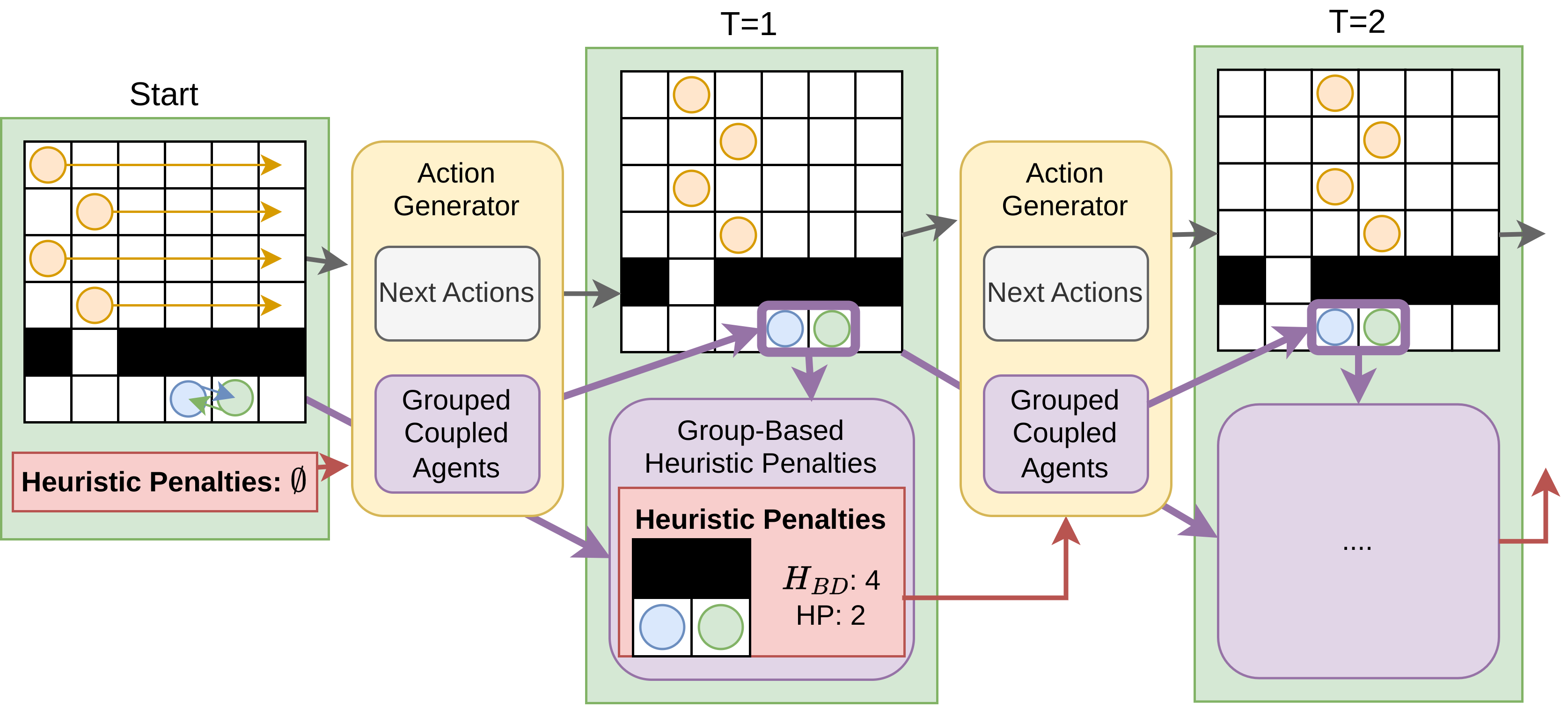
Figure 1: The iterative planning, execution, and grouped heuristic updates/penalties for Windowed Complete MAPF (WinC-MAPF).

3.1 Planning in Joint-State Space

Our first observation is to leverage existing Real-Time search literature that has been solely explored in single-agent planning as mentioned in Section 2.3. We can directly leverage single-agent Real-Time search literature if we view our multi-agent problem in the joint space.

We formally redefine the windowed MAPF planning problem from this joint-space perspective. Given $N$ agents, we define a joint configuration $\mathcal{C}^{t}=[s_{1}^{t},...s_{N}^{t}]$. At every timestep, we query a high-level “action-generator” to return a sequence of configurations $\Pi^{0:W}=[\mathcal{C}^{0},...\mathcal{C}^{W}]$ which minimizes $|\Pi|=|\Pi^{0:W}|+|\Pi^{W:T_{max}}|=\sum_{t=0}^{W-1}c(\mathcal{C}^{t},\mathcal{C}^{t+1})+h_{BD}(\mathcal{C}^{W})$. We define the joint cost and heuristic intuitively, $c(\mathcal{C},\mathcal{C}^{\prime})=\sum_{i}^{N}c(s_{i},s_{i}^{\prime})$ and $h_{BD}(\mathcal{C})=\sum_{i}^{N}h^{*}_{i}(s_{i})$ (BD = Backward Dijkstra).

To re-iterate, the advantage of this interpretation is that we have converted our windowed MAPF problem into a standard single-agent real-time search problem. Thus given this sequence of configurations, we apply a standard Bellman Update to the heuristic of $\mathcal{C}$ via $h(\mathcal{C})\leftarrow c(\mathcal{C},\mathcal{C}^{H})+h(\mathcal{C}^{H})$. Given a timestep $t$ and configuration $\mathcal{C}^{t}$, we move our agents to $\mathcal{C}^{t+1}$, update our heuristic of $\mathcal{C}^{t}$, and repeat.

$h(\mathcal{C})$ is initially set to $h_{BD}(\mathcal{C})$ and gradually increases as agents visit states. Instead of calling these changes heuristic updates, we use the term “heuristic penalty” to describe how the heuristic for visited states increases when we apply our update equation. This effectively “penalizes” those states and encourages the search to explore other states. A heuristic penalty state is a state $\mathcal{C}$ which has a non-zero increase from the base heuristic value, i.e. $h(\mathcal{C})=h_{BD}(\mathcal{C})+h_{p}(\mathcal{C})$ where the penalty $h_{p}(\mathcal{C})>0$. Our penalty update equation is then $h_{p}(\mathcal{C})=c(\mathcal{C},\mathcal{C}^{\prime})+h(\mathcal{C}^{\prime})-h_{BD}(\mathcal{C})$.

Now during execution, if the MAPF instance is stuck in deadlock at some location $\mathcal{C}$, we can show that the heuristic $h(\mathcal{C})$ will continually increase. Thus after enough iterations, the action generator which minimizes $\operatorname*{arg\,min}_{\mathcal{C}^{\prime}}c(\mathcal{C},\mathcal{C}^{\prime})+h(\mathcal{C}^{\prime})$ will eventually choose a different state (i.e. the chosen $\mathcal{C}^{\prime}\neq\mathcal{C}$) as $h(\mathcal{C})$ will be too large, and leave the deadlock.

Quickly recapping, we view the windowed MAPF problem as a real-time problem in the joint space, requiring an “action-generator” that reasons about $h(\mathcal{C})=h_{BD}(\mathcal{C})+h_{p}(\mathcal{C})$. However, existing MAPF methods like Prioritized Planning, CBS, and LaCAM do not reason about this $h(\mathcal{C})$ out of the box. We show how this can be done for CBS in Section 4.

3.2 Reasoning about Coupled Agents

The framework we have described so far suffers from an obvious issue; the size of the joint state-space $\mathcal{C}$ is very large. Consequently, escaping local minima, which in our context are agents stuck in deadlock/livelock, can be challenging. The process often requires filling in large heuristic depressions, which can lead to poor performance as the agent may remain stuck in the minimum for extended periods before finding a way out.

Concretely, imagine we have the starting configuration as depicted in Figure 1 (where the goals are indicated with arrows). Note that the blue and green agents on the bottom want to swap locations. The main observation is that the orange agents and the blue/green agents are independent even though they are on the same connected graph. However, iteratively planning and computing heuristic penalties on the joint configurations as described will result in the action generator wanting to avoid the exact joint configurations penalized. Thus, the AG could request the orange agents to move, encountering new configurations without penalties, even though the underlying blue-green deadlock remains. To resolve this deadlock, the current framework requires the AG to search over all agent’s locations even though we intuitively know it should focus on just the blue and green agents.

Our key idea is therefore to apply the heuristic penalty to specific groups of agents instead of on the entire joint-state space. In Figure 1, this means that instead of applying $h$ on the single state $\mathcal{C}$, we can determine the specific groups of agents (e.g. blue and green) and only attribute the heuristic penalty to them. Conceptually, the idea is that if each agent $i$ was able to move from $s$ to their optimal next state $s^{\prime}$, there would be no heuristic penalty as each $h_{i}(s)=c(s,s^{\prime})+h_{i}(s^{\prime})$ due to the heuristic being a perfect single-agent heuristic. Thus, $h_{p}(\mathcal{C})>0$ means there exists at least one agent $i$ with $h_{i}(s)<c(s,s^{\prime})+h_{i}(s^{\prime})$ unable to move to its best location. Additionally, this agent $i$ must be blocked by some other agent $j$. Thus, instead of updating the heuristic of $\mathcal{C}$, we can update $\mathcal{C}_{Gr=\{i,j\}}$ (assuming no other agents are interacting with $i,j$).

Our objective is, given a $\mathcal{C},\mathcal{C}^{\prime}$ transition, to detect these groups of agents and apply heuristic penalties to just the group of agents rather than the entire joint-state space. Concretely, for each agent we determine which other agents it is directly interacting with. Agents that are able to do their best action, and whose best action does not block another agent’s movement, are “independent” to all other agents. On the flip side, agents that cannot do their best action due to another agent are coupled with the impeding agents.

One crucial observation is that it can be non-trivial to determine which agents are coupled once the action generator returns the next state. Agents could be next to each other but still independent, or on the flip side be non-adjacent but coupled. However, instead of reasoning about coupled agents after the action generator, we can use the action generator itself as it must have reasoned about agent interactions to return a valid next action. All modern MAPF heuristic search planners reason about agent interactions internally, e.g. M* explicitly couples agents that intersect (Wagner and Choset 2011), PIBT’s priority inheritance reasons about colliding agents, and CBS resolves conflicts between intersecting agents. Thus, we require that the action generator additionally returns groups of interacting agents. We highlight that this can be generally done with bookkeeping and without much added compute to existing MAPF solvers.

Given a joint configuration $\mathcal{C}$ and a set of HPs for groups of agents at various $\mathcal{C}_{Gr}$, we then compute $h(\mathcal{C})=h_{BD}(\mathcal{C})+\sum_{i}h_{p}(\mathcal{C}_{Gr_{i}})$ for a disjoint set of groups whose locations match the configuration.

3.3 Overall WinC-MAPF Framework

Thus, we require the AG to incorporate $h(\mathcal{C})$ updates when reasoning about which actions to execute as well as detect the coupled agents for the chosen actions. We focus on optimal windowed action generators that determine the action sequence minimizing $\operatorname*{arg\,min}_{C^{\prime}}c(\mathcal{C},\mathcal{C}^{\prime})+h(\mathcal{C})$. We show in our proof in the appendix that these AGs retain completeness guarantees even though they plan partial paths. Future work could show how certain non-optimal windowed AGs could still retain completeness guarantees in our framework.

Theorem 1.

Given a finite undirected search space and: (1) the initial heuristic is admissible, (2) our AG picks $\mathcal{C}^{\prime}=\operatorname*{arg\,min}c(\mathcal{C},\mathcal{C}^{\prime})+h(\mathcal{C}^{\prime})$ and identifies coupled agents groups, then WinC-MAPF with its grouped update equation is complete (i.e. all agents will eventually reach their goals if a solution exists).

We can now effectively plan in the composite state-space while applying heuristic penalties to groups of agents. Algorithm 1 describes this procedure. We have a set of Heuristic Penalties (line 2) which we pass into the AG with the current configuration (line 4). The AG returns the next configuration (or actions leading to it) as well as a list of agent groups. For each group $Gr$, we compute the update equation with respect to the group’s joint configuration $\mathcal{C}_{Gr}$ and if it is greater than 0, we add the subgroup configuration and penalty into our library of heuristic penalties. Then, we move agents to the picked locations and replan.

Algorithm 1 Windowed Complete MAPF Framework

1:procedure Windowed Complete MAPF($\mathcal{C}^{cur}$)

2:     $\mathcal{H}\leftarrow\emptyset$ $\triangleright$ Heuristic Penalties

3:     while $\mathcal{C}^{cur}\neq$ Goal do

4:         $\mathcal{C}^{\prime}$, ListOfGroups = AG($\mathcal{C}^{cur}$, $\mathcal{H}$)

5:         for $Gr$ $\in$ ListOfGroups do $\triangleright$ For each group

6:              $h_{new}=c(\mathcal{C}^{cur}_{Gr},\mathcal{C}_{Gr}^{\prime})+h(\mathcal{C}_{Gr}^{\prime})$

7:              $penalty=h_{new}-h_{BD}(\mathcal{C}^{cur}_{Gr})$

8:              if $penalty>0$ then

9:                  $\mathcal{H}$.insert($\mathcal{C}^{cur}_{Gr}$, $penalty$)                        

10:         $\mathcal{C}^{cur}\leftarrow\mathcal{C}^{\prime}$ $\triangleright$ Move agents      

The main assumptions we have currently is that we have a centralized AG and we have a perfect backward Dijkstra heuristic for each agent. The first assumption allows the AG to reason about heuristic penalties between coupled agents. The second assumption is not strictly required but simplifies the problem as we do not need to do single-agent heuristic updates. Both of these assumptions are common in current MAPF literature, and prior work has shown that for certain state-of-the-art methods like LaCAM, a perfect backward Dijkstra heuristic is required (Veerapaneni et al. 2024). Both these assumptions can be relaxed in future work.

The next section describes Single-Step CBS, an action generator that satisfies the two properties required by WinC-MAPF (identifying agent groups and optimally solving a windowed problem).

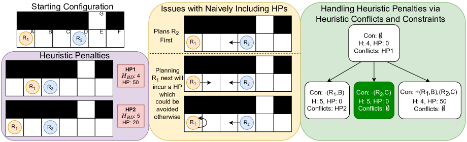
Figure 2: We depict an illustrative situation where Single-Step CBS needs to determine the best joint configuration to move agents to given heuristic penalties (left). Section 4.1 walks through this figure and describes how naively incorporating heuristic penalties in CBS results in incorrect solutions (middle). Our innovation is to introduce “heuristic conflicts” which allows SS-CBS to find the optimal solution (right).

4 Single-Step CBS

We want to design a windowed solver that incorporates heuristic penalties and optimally solves $W=1$, i.e. finds the next best step that minimizes $c(\mathcal{C},\mathcal{C}^{\prime})+h(\mathcal{C}^{\prime})$. We note that in MAPF with $N$ agents and an individual action space of size 5, naively computing this requires generating all $5^{N}$ possible neighboring configurations as certain configurations may have heuristic penalties. Thus we employ CBS to intelligently find the optimal single-step configuration.

Since we want a windowed solver with $W=1$, Single-Step CBS (SS-CBS) only considers conflicts within the first timestep. However, regular CBS does not operate in the joint configuration space of MAPF problems and instead exploits the structure of MAPF to iteratively plan agents individually. One key assumption in CBS is that it can minimize the joint $c(\mathcal{C},\mathcal{C}^{\prime})+h(\mathcal{C}^{\prime})$ by minimizing individual $c(s,s^{\prime})+h(s^{\prime})$ subject to constraints. Thus, incorporating HPs which work on the joint configuration of multiple coupled agents breaks this assumption and requires careful reasoning. Our main innovation lies in modifying SS-CBS to return the optimal solution given heuristic penalty updates. A minor additional modification is returning groups of conflicting agents.

4.1 Handling Heuristic Penalties with Constraints

Incorporating updates to $h$ via heuristic penalties is non-trivial in CBS. A naive way to incorporate a heuristic penalty in CBS is to plan CBS normally and just add the heuristic penalty cost to CT nodes whose configurations match the penalty. However, we show that this fails to find an optimal solution. A second naive way is to incorporate the penalty in the low-level search. We show how this similarly fails. The core conceptual issue with naively incorporating heuristic penalties is that the high-level/low-level is not fully aware of the heuristic penalties until after it has planned paths, so it is unable to avoid them beforehand.

Figure 2 depicts Single-Step CBS in a scenario where two agents want to swap their location from their starting configuration ($R_{1},R_{2}$ want to reach $D,A$ respectively, top left). The left purple box shows two Heuristic Penalties with their corresponding configurations and penalty values (50 and 20 respectively). We created the two HPs for this example; in the real system, HPs would be created from previous iterations of execution and applying the subgroup logic and update equation described in Section 3.2. Given the starting configuration and the two HPs, SS-CBS needs to find the optimal next configuration that minimizes $c(\mathcal{C},\mathcal{C}^{\prime})+h(\mathcal{C}^{\prime})$. Since the cost of all actions is 1, $c(\mathcal{C},\mathcal{C}^{\prime})=2$ regardless of the chosen $\mathcal{C}^{\prime}$ configuration. Thus, we focus on minimizing $h(\mathcal{C}^{\prime})$. In our example, the optimal next configuration is $(R_{1},B),(R_{2},D)$ which has a heuristic of 5.

Incorrect: Incorporating HPs in High Level The most obvious way to incorporate HPs is to add them to the CT node’s heuristic if the CT node’s configuration matches the penalty. This fails as the penalty is applied after the low-level planning occurs, so the low-level planner does not avoid HPs in the beginning.

We take a look at generating the root CT node in our example (middle yellow box). If the root node first plans $R_{2}$, then $R_{2}$ moves to $C$ as this reduces its heuristic (middle box, top row). We do not incur a HP as we do not know the configuration of $R_{1}$ yet. When we plan $R_{1}$, the low-level search has $R_{1}$ minimize its single agent heuristic and move to $B$ which results in the root CT node with $(R_{1},B),(R_{2},C)$ (middle box, middle row). This then incurs HP1’s penalty of 50. Note that there are no agent conflicts and thus CBS will return this solution with a net-heuristic of $4+50=54$. This is substantially worse than the true solution.

Incorrect: Incorporating HPs in Low Level On the flip side, we could attempt to incorporate the heuristic penalty in the low-level search. When replanning an agent, we know the location of all other agents, so the low-level search can check if certain configurations would incur a heuristic penalty. However, this fails as the first agents that plan in the root CT node do not know the locations of other agents that haven’t been planned yet. As a result, they plan greedily, potentially forcing later agents into suboptimal situations.

Like before, we can plan $(R_{2},C)$ which does not incur any penalty as we do not have $R_{1}$’s position. When planning for $R_{1}$, we know $(R_{2},C)$ and the search will penalize $(R_{1},B)$ by HP1 and instead picks $(R_{1},A)$ which is only penalized by HP2 (middle box, bottom row). This results in a net heuristic of $5+20=25$ which is again not optimal.

Solution: Introducing “Heuristic Conflicts” Our idea is thus not to incorporate the heuristic penalty immediately. Instead, when CBS encounters a joint configuration that would incur a penalty, it marks the CT node with a “heuristic conflict” without adding the penalty into the CT node’s heuristic value yet. Formally, a heuristic conflict occurs when agents’ positions match the positions of a HP. Resolving the heuristic conflict requires applying regular (negative) vertex constraints on each agent in the heuristic conflict which forces them to avoid the joint configuration (and thus penalty) as well as one CT node with positive vertex constraints which requires the agents to be at the penalty joint-configuration and only then incurring the HP.

In our example, the agents plan independently like usual and the root node has no vertex or edge conflicts. However, we detect that HP2 could apply and create the corresponding heuristic conflict (right box, top CT node). We then generate three child nodes, the first two CT nodes with negative vertex constraints and the last one with multiple positive vertex constraints. We see how this results in the optimal configuration being found (highlighted in green). Thus given an HP with $K$ agents, our heuristic constraint will generate $K$ children with a single additional negative vertex constraint and one child with $K$ additional positive vertex constraints.

4.2 Detecting Heuristic Agent Groups

SS-CBS should also return groups of agents that are coupled. Our main observation is that agent conflicts directly denote coupled agents. If agents are directly coupled, they must have a conflict between them that got resolved. Similarly, independent agents will not conflict with each other.

There is the possibility of indirect interactions. In particular, $R_{1}$ could conflict with $R_{2}$, causing $R_{2}$ to replan which then conflicts with $R_{3}$. In this case, $R_{1}$’s action of $R_{2}$ directly caused an interaction with $R_{3}$, so $R_{1}$ and $R_{3}$ are indirectly coupled. Thus we can determine disjoint groups of dependent agents by first generating non-disjoint groups of agents for each resolved conflict and then merging groups with shared agents. In our example, we start with $(R_{1},R_{2})$ and $(R_{2},R_{3})$ and will end with $(R_{1},R_{2},R_{3})$ after merging.

We note that we only care about resolved conflicts that occur on CT nodes on the one branch that led to the outputted joint state. Conflicts in other branches do not affect the movements of agents in the outputted joint state. Thus, agents in vertex, edge, or heuristic conflicts on the CT branch to the goal node will be grouped together.

4.3 Subtleties

A powerful technique for speeding up CBS is Enhanced CBS (Barer et al. 2014) which replaces the low-level and high-level optimal searches with bounded-suboptimal focal searches. Thus, an obvious idea to potentially improve SS-CBS is to introduce these focal searches. As stated in Section 3.3, our proof of completeness only applies to optimal AGs. Hence we set $w_{so}=1$ which results in only using the focal search for tie-breaking. For experimental curiosity, we include results for SS-CBS with a suboptimal high-level search in the appendix (although we do not prove completeness for this suboptimal AG).

We have two additional subtleties. First, there is an important implementation nuance for determining which HP to apply to a configuration if multiple HPs were applicable. Second, we introduced a tiebreaking mechanism that, when faced with two solutions of equal cost, prioritizes reducing the heuristic of some agents over others. Due to space constraints, the details are included in the appendix.

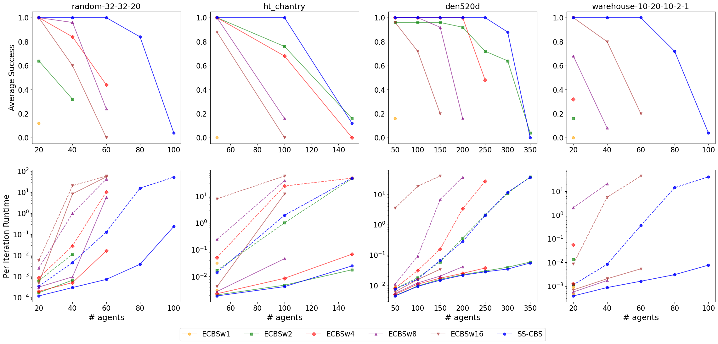
Figure 3: We compare our method SS-CBS (blue), which has $w=1$, against windowed ECBS with different window sizes $w=\{1,2,4,8,16\}$. SS-CBS is theoretically complete (windowed ECBS is not) and also outperforms windowed ECBS empirically.

5 Experiments

Our experiments demonstrate the empirical performance of our theoretically complete SS-CBS algorithm. We first evaluate SS-CBS on standard benchmark maps (Stern et al. 2019) and observe that SS-CBS is indeed able to outperform the windowed baselines. We then evaluate SS-CBS on high-congestion small maps and showcase SS-CBS’s superiority in this regime. Our appendix contains additional analysis and results. We highlight that there do not exist any complete windowed baselines. We thus compare against windowed ECBS with window $w=\{1,2,4,8,16\}$. For consistency with SS-CBS, we use a suboptimality factor of $w_{so}=1$ for ECBS and no additional CBS improvements.

5.1 Benchmark Scenarios

Figure 3 shows the results of SS-CBS compared to windowed ECBS without heuristic penalties. We evaluate on 4 benchmark maps (each column: random-32-32-20, ht_chantry, den520d, warehouse-10-20-10-2-1) with a 1 minute timeout across 25 scenarios. We additionally end windowed ECBS in failure when it repeats previously visited configurations 100 times (i.e. deadlock or livelock).

The first row shows how SS-CBS (blue) has an almost strictly better performance than the windowed ECBS baselines. We first highlight that the performance of Windowed ECBS depends significantly on the map, with no single window value dominating. Windowed ECBS with $w=1,2$ sometimes perform poorly due to their small window size which leads to deadlock/livelock, while $w=8,16$ sometimes suffer from large runtimes. SS-CBS is able to consistently perform better than the corresponding windowed ECBS method even though SS-CBS plans only a single step. SS-CBS’s performance on warehouse-10-20-2-1 shows how it performs well in scenarios that require long-term planning (as shown by Windowed ECBS requiring a larger window size to have non-trivial success rate).

The second row shows the per-iteration runtime of each method, with the median runtime in solid and the maximum (longest) iteration runtime in dashed. The difference between the median and maximum highlights how congested iterations can take a significant amount of time (e.g. 10s of seconds for one optimal step) compared to typical iterations. We observe how SS-CBS’s runtime is usually in line with ECBS $w=1,2,4$ and substantially smaller than $w=8,16$.

The solution cost of SS-CBS was roughly 2-8% higher than windowed ECBS. We observed that across all maps, the number of HPs created by SS-CBS grew roughly linearly along with the number of agents, but the number of HPs encountered in the CT grew exponentially.

5.2 Tough Congested Scenarios

The previous section shows how SS-CBS can outperform windowed ECBS in standard benchmark scenarios. We were additionally interested in SS-CBS’s performance in extremely congested scenarios and thus evaluated it on small maps with high congestion from Okumura (2022).

Table 1 shows the average success from 20 seeds with a timeout of 1 minute, with the number $N$ in parenthesis denoting using the first $N$ agents in a scenario. We see how windowed ECBS with window sizes $1,2,4,8,16$ fails completely. Additionally, we compared it to EECBS (Explicit Estimation high-level search) with all CBS improvements, including bypass, symmetry reasoning, prioritized conflicts, and full horizon planning. Despite these enhancements, EECBS still struggles due to high congestion.

SS-CBS can solve nearly all problems with high accuracy. It’s worth emphasizing that SS-CBS uses no CBS improvements, relying solely on basic focal search with $w_{so}=1$ and planning just a single step at a time. Despite this, it outperforms both windowed ECBS and EECBS baselines. Additional results in the appendix further compare SS-CBS to EECBS, demonstrating that SS-CBS is at least an order of magnitude faster on solved instances.

SS-CBS’s performance demonstrates two key points. First, its high success rate on these challenging, congested maps shows how heuristic penalties can effectively guide SS-CBS to bypass complex congestion. Second, EECBS struggles due to the high number of conflicts in these scenarios. SS-CBS’s success highlights how iterative single-step planning with heuristic updates can be an effective approach for resolving difficult congestion issues. All existing windowed methods produce congestion due to their myopic planning. Thus, SS-CBS improving performance with windowed planning in severe congestion is remarkable.

6 Conclusion and Future Work

Existing MAPF works have focused on designing methods to solve full-horizon planning. When faced with shorter deadlines, all current methods take the full horizon MAPF methods and simply reduce the planning horizon to a smaller window. This has been shown to cause deadlock/livelock/insurmountable congestion due to the limited planning horizon. We introduce WinC-MAPF, the first framework that enables theoretical completeness with windowed MAPF solvers. In particular, we show that using windowed “Action Generator” that incorporates heuristic penalties, identifies agent groups, and optimally minimizes $c(\mathcal{C},\mathcal{C}^{\prime})+h(\mathcal{C}^{\prime})$ is complete. Following this framework, we designed SS-CBS which uniquely introduces “heuristic conflicts” to successfully incorporate heuristic penalties and return the optimal next step action. We experimentally validate how our theoretically complete method actually translates to real performance benefits with SS-CBS consistently outperforming windowed ECBS across a variety of windows and maps.

We are very excited about future work that can relax the limitations of our framework. First, the most useful extension is to incorporate and prove completeness for bounded suboptimal AGs within our framework. This can allow more solvers such as PIBT, MAPF-LNS2 (Li et al. 2022), W-EECBS (Veerapaneni, Kusnur, and Likhachev 2023), or even using a learnt neural network policy. Second, one obvious extension is to generalize SS-CBS to work on longer horizons. This also opens the door to using more sophisticated real-time heuristic update methods. Third, future work could try to relax the perfect backward Dijkstra single-agent heuristic assumption and learn individual heuristics online.

Planning partial paths rather than full paths is a significant target that researchers need to achieve for their methods to be used in real systems. We believe the WinC-MAPF framework and SS-CBS are a significant step towards bridging this gap and enabling effective windowed MAPF solvers.

Appendix A Quick Summary

Recommended background readings

Readers new to MAPF or (E)CBS are recommended to read ECBS (Barer et al. 2014). Readers unfamiliar with windowed MAPF solvers should read Rolling-Horizon Collision Resolution (Li et al. 2020). Readers new to Real-Time Heuristic Search can take a look at LRTA* in Korf (1990).

Motivation in respect to prior work:

The majority of MAPF methods which find entire collision free paths to goal can take a long time (e.g. $>10$ seconds). Real-world practitioners cannot wait this long. Thus to reduce planning time, existing works only reason about collisions within a fixed time window/horizon, where the window $W$ is much smaller than the entire solution path.

A key issues with these windowed approaches is that their myopic planning results in deadlock or livelock if their window is too small. Table 1 shows examples where windowed MAPF solvers fail in congestion which requires longer horizon planning. More broadly, all existing windowed MAPF solvers regardless of window size lack theoretical completeness and several windowed works have explicitly cited deadlock as a key issue in their experiments (Li et al. 2020; Okumura et al. 2022; Jiang et al. 2024).

Intended Takeaways

1. Windowed Complete MAPF (WinC-MAPF) Framework: We develop the first general framework that enables creating windowed MAPF solvers that have completeness guarantees. Our first insight is that we can leverage the single-agent Real-Time Heuristic Search perspective which uses limited horizon/windowed planning but maintains completeness by updating the heuristics of visited states. Our second insight is to leverage the semi-independence of agents in MAPF and only computing the heuristic updates in-respect to groups of coupled agents rather than the entire joint configuration space.

Formally, we define a windowed MAPF “Action Generator” (AG) as a search method that given a window $W$ and a current configuration $\mathcal{C}$, finds a $\mathcal{C}^{\prime}$ (and associated actions) that is a valid neighboring configurations within $W$ timesteps. Additionally, the AG needs to determine groups of coupled agent groups as defined in Section 3.2. We prove in the next section how an optimal windowed AG that computes $\operatorname*{arg\,min}c(\mathcal{C},\mathcal{C}^{\prime})+h(\mathcal{C}^{\prime})$ is complete under standard conditions which regular MAPF holds. It is likely possible that suboptimal AG’s, e.g. ones that do not exactly find the argmin but some bounded suboptimal AG, will be complete but we were unable to prove that using standard techniques and is left for future work.

2. Single-Step CBS (SS-CBS): We develop SS-CBS which is an instantiation of CBS following our WinC-MAPF framework. SS-CBS finds the optimal next step (so window $W=1$) given heuristic updates. We show that naively incorporating heuristic updates (which we redefine in respect to heuristic “penalties”) by adding it into the high-level or low-level CBS search is incorrect. SS-CBS’s innovation is to incorporate heuristic penalties by introducing a new “heuristic conflict” and constraint that defers the addition of the heuristic penalty and enables all agents to replan to avoid a penalty. We additionally show how SS-CBS can easily determine coupled agent groups by merging pairs of conflicting agents.

Experimentally, Figure 3 shows how SS-CBS has a higher success rate and agent scalability on standard MAPF benchmark maps when compared to windowed ECBS across a windows $w=\{1,2,4,8,16\}$. We highlight that SS-CBS plans only one single-step (i.e. extremely myopic planning) but is able to handle congestion/deadlock better. Additionally, we investigate the performance of these windowed methods tough small scenarios (Table 1, A1). In these scenarios, we find that windowed ECBS methods uniformly fail, and that even EECBS with all optimizations struggles. SS-CBS is able to almost perfectly solve these instances. All existing windowed MAPF methods struggle in congestion, so SS-CBS’s superior performance in these congested scenario highlights the power of the WinC-MAPF framework.

Main Limitations and Future Improvements

1. SS-CBS’s main limitation is that although most iterations are fast ($<$0.1 seconds), Figure 3 shows how a few iterations can take a significant amount of time (e.g. $>$10 seconds) when congestion increases. Future work should improve the runtime of SS-CBS.

2. SS-CBS requires a perfect single-agent heuristic. Although several other MAPF methods requires this (e.g. PIBT/LaCAM (Veerapaneni et al. 2024)), this is not generally required for CBS and future work could relax this.

3. SS-CBS plans a single step. Future work can extend SS-CBS to planning multiple steps.

4. As mentioned earlier, our WinC-MAPF currently proves completeness with an optimal AG. We conjecture that future work can likely modify and prove that bounded suboptimal AG’s can be complete within our framework.

Appendix B Proving Completeness of WinC-MAPF with Agent Group Heuristic Penalties

A key idea of WinC-MAPF is to compute heuristic penalties on groups of agents rather than the entire joint configuration. Without this, i.e. if we just computing heuristic penalties on the full joint configuration space, we get completeness by directly applying the single-agent proof. We thus first define agent groups. We then roughly restate the standard proof used in the original real-time search LRTA* paper (Korf 1990) to provide context on the differences that our WinC-MAPF framework has in respect to proving completeness. We cannot directly use LRTA*’s proof. Instead, we can use the fact that this proof shows how (1) proving that an algorithm doesn’t cycle infinitely proves completeness and (2) how heuristic values with cycles with an update of $h^{\prime}(s_{i})\leftarrow c(s_{i},s_{i+1})+h(s_{i+1})$ results in infinitely large heuristic values. We then show how our heuristic values are admissible, which combined with (1) and (2) with optimal windowed AGs result in our framework being complete.

B.1 Agent Groups

The general definition of a group of coupled agents is a set of agents where for each agent $R_{i}$, there exists an $R_{j}$ that either blocks its path or vice-versa. From an abstract perspective, we can compute this by iterating through each agent which is not on its optimal single-agent path and storing the ids of the other agents which prevented it from picking a better path (there must exist at least one other agent otherwise the agent could have gone on its optimal path). This builds a dependency graph where agents that share an edge $R_{i}\rightarrow R_{j}$ denote $R_{i}$ blocked by $R_{j}$.

We can then find all the disjoint connect components in this dependency graph (e.g. via a DFS) where each disjoint connected component depicts a group of agents that are blocking each other. Instead of doing $h(\mathcal{C})\leftarrow c(\mathcal{C},\mathcal{C}^{\prime})+h(\mathcal{C}^{\prime})$, we do $h(\mathcal{C}_{Gr})\leftarrow c(\mathcal{C}_{Gr},\mathcal{C}_{Gr}^{\prime})+h(\mathcal{C}_{Gr}^{\prime})$ for each group of agents $Gr$ at configuration $\mathcal{C}_{Gr}$.

B.2 Standard Single-Agent Real-Time Search Completeness Proof

LRTA* (Korf 1990) is a single agent algorithm where at each timestep, the agent picks $\operatorname*{arg\,min}_{s^{\prime}}c(s,s^{\prime})+h(s^{\prime})$ over successor states $s^{\prime}$ and updates the heuristic $h^{\prime}(s)\leftarrow c(s,s^{\prime})+h(s^{\prime})$. We summarize its proof of completeness.

Theorem 2.

In a finite problem space with positive edge costs and finite heuristic values, in which a goal state is reachable from every state, LRTA* will find a solution.

Proof.

In a finite state space, if LRTA* does not reach the goal, there must exist a finite cycle that LRTA* is stuck in (otherwise it will visit new states and eventually the goal).

Suppose LRTA* is stuck in a finite cycle of length N consisting of $s_{1},s_{2},...,s_{N}$, and is at $s_{1}$. When moving to the next state $s_{2}$, it updates $h^{\prime}(s_{1})\leftarrow c(s_{1},s_{2})+h(s_{2})$. Our objective is to show that when traversing the cycle once, at least one state $s_{i}$ has their heuristic value increase. If so, then over an infinite amount of cycling, the heuristic values of at least one state $s_{i}$ in the cycle will become infinitely large. Then when LRTA* is at $s_{i-1}$ and does a 1-step lookahead, it will pick a different state and exit the cycle.

Suppose LRTA* travels the cycle but for all $s_{i}$ we have that $h^{\prime}(s_{i})\leftarrow c(s_{i},s_{i+1})+h(s_{i+1})=h(s_{i})$. This implies that $h(s_{i})>h(s_{i+1})$ as $c(s_{i},s_{i+1})>0$. This occurs over all $s_{i}$ which leads to $h(s_{1})>h(s_{2})>...>h(s_{N})>h(s_{1})$ which is a contradiction. Therefore there must be some state that gets its heuristic value increased, e.g. $\exists s_{i}$ s.t. $h^{\prime}(s_{i})\leftarrow c(s_{i},s_{i+1})+h(s_{i+1})>h(s_{i})$.

LRTA* is therefore guaranteed to eventually leave any finite cycle. Since a finite problem space has a finite set of cycles that do not include the goal, LRTA* at worst will explore all of these and eventually exit them and reach the goal. ∎

B.3 WinC-MAPF Proof

From a high level, the LRTA* proof proves completeness by showing that in a cycle and given the update $h^{\prime}(s_{i})\leftarrow c(s_{i},s_{i+1})+h(s_{i+1})$, the heuristic values in the cycle must increase infinitely large to the extent that LRTA* will pick a different $s_{i}^{\prime}$ that avoids the large heuristic value. This requires/assumes that only heuristic values in the cycle increases while other heuristic values do not.

A key idea of WinC-MAPF is to compute heuristic penalties on groups of agents rather than the entire joint configuration. Note that without this, i.e. if we just computing heuristic penalties on the full joint configuration space, we get completeness by directly applying the single-agent proof. Thus, using heuristic penalties on groups complicates the proof of completeness as when computing/creating a heuristic penalty, we are increase the heuristic values of joint-states not in the cycle. We unfortunately cannot use this proof.

Instead, we prove completeness in Theorem 1 by showing how our overall heuristic values are always admissible. If we can show this, then we are guaranteed to not cycle infinitely as this will infinitely increase some heuristic value and contradict our admissible heuristic value guarantee.

Theorem 3.

Given a finite undirected search space and: (1) the initial heuristic is admissible, (2) our AG picks $\mathcal{C}^{\prime}=\operatorname*{arg\,min}c(\mathcal{C},\mathcal{C}^{\prime})+h(\mathcal{C}^{\prime})$ and identifies coupled agents groups, then WinC-MAPF with its grouped update equation will always have admissible heuristic values for all $\mathcal{C}$.

We calculate the joint heuristic value by summing up mutually exclusive group heuristic penalties as described in Section C.1. If we can prove that the group heuristic values are admissible, then the sums of disjoint grouped heuristic values is also admissible as groups interacting can only increase the true cost-to-go. Thus we prove the following lemma.

Lemma 1.

Given a finite undirected search space and: (1) the initial heuristic is admissible, (2) our AG picks $\mathcal{C}^{\prime}=\operatorname*{arg\,min}c(\mathcal{C},\mathcal{C}^{\prime})+h(\mathcal{C}^{\prime})$ and identifies coupled agents groups, then WinC-MAPF with its grouped update equation will always have admissible heuristic values for all group configurations $\mathcal{C}_{Gr}$.

Proof.

We prove this via induction. Our inductive hypothesis is that we have $h(\mathcal{C}_{Gr})\leq h^{*}(\mathcal{C}_{Gr})$ across all grouped agent $Gr$ configurations $\mathcal{C}_{Gr}$ and iterations of running our Windowed MAPF framework.

Base case: Our initial group heuristic values, the sum of each agent’s backward Dijkstra distance, is admissible as interactions between agents can only increase the solution cost. Thus over all groups of agents, the joint heuristic value is admissible.

Inductive Step: We assume that at some timestep $T$ at $\mathcal{C}$, all the heuristic values are admissible. The AG picks a $\mathcal{C}^{\prime}$ that minimizes $c(\mathcal{C},\mathcal{C}^{\prime})+h(\mathcal{C}^{\prime})$. Then for each coupled group of agents, we update the group’s joint-configuration (via our heuristic penalty) to $h(\mathcal{C}_{Gr})\leftarrow c(\mathcal{C}_{Gr},\mathcal{C}_{Gr}^{\prime})+h(\mathcal{C}_{Gr}^{\prime})$.

Suppose that there is a group of agents $GrA$ at $\mathcal{C}_{GrA}$ whose heuristic value becomes inadmissible. This means that the chosen $\mathcal{C}_{GrA}^{\prime}$ was not optimal and there existed a different $\mathcal{C}_{GrA}^{*}$ that was optimal. However, since we are running on optimal AG, we would have replaced $\mathcal{C}_{GrA}^{\prime}$ with $\mathcal{C}_{GrA}^{*}$. If this did not interact with any other agents, this would reduce our overall cost without changing any other agents positions/actions and contradict the optimal AG. If it did interact with other agents, then $GrA$ would need to be larger and include these other agents, violating our definition of groups. Thus, neither of these are possible. This means that our heuristic value stays admissible for all groups after updating. ∎

Appendix C SS-CBS

C.1 Subtleties

Determining Which HPs to Apply

As discussed earlier, give a CT node we need to detect heuristic conflicts. This can be done by going through all the heuristic penalties and checking if their agent locations match with the CT’s configuration.

However, a non-trivial issue occurs as it is possible that multiple non-disjoint heuristic conflicts could be detected. For example, a configuration could have a heuristic penalties involving $(R_{1},R_{2})$ and another involving $(R_{2},R_{3})$. We cannot apply both as this would double count the heuristic penalty involving $R_{2}$. Thus more broadly, we cannot apply multiple non-disjoint heuristic conflicts as if we were to resolve all of them, this will over-count the heuristic penalty.

Technically, given a set of possible heuristic penalties, we could try to maximize the combination of these penalties such that chosen penalties do not have overlapping agents. This ends up being a maximum weighted disjoint set-cover problem where each heuristic penalties is a set and the set’s weight is the penalty. We note that solving just disjoint set-cover is NP-Complete (Cardei and Du 2005), so solving this efficiently is hard. We thus instead do a greedy approximation and choose to apply the heuristic conflict with the highest penalty.

One important implementation note is that initially we greedily chose the highest HP that was mutually exclusive (i.e. did not share agents) with prior chosen HPs. This is wrong and resulted in deadlock as the order in which HPs are chosen affects the solution. In certain deadlock locations, say $(R_{1},R_{2},R_{3})$, SS-CBS would always first encounter an HP with $(R_{1},R_{2})$ and apply that. Then later in the same CT search, $(R_{1},R_{2},R_{3})$ is encountered but we did not apply an HP as $R_{1}$ and $R_{2}$ are already used up. This resulted in SS-CBS repeatedly picking the deadlock location as even though $(R_{1},R_{2},R_{3})$ accumulated large penalties, SS-CBS would only apply the $(R_{1},R_{2})$ penalty.

Thus, every time we compute heuristic penalties and conflicts, we recompute it from scratch while maintaining consistency with prior vertex constraints. This allows us to initially pick $(R_{1},R_{2})$ and then afterwards “reassign” $(R_{1},R_{2},R_{3})$ later on.

Tie-Breaking

Given the 1-step plans, it is likely that there are many SS-CBS solutions with an equally good cost. We found it helpful to tiebreak by introducing agent “priorities”. The intuition behind this is that given an symmetric situation of two agents in a hallway (where all adjacent configurations have the same summed $h$ value), we prefer one agent to “push” the other agent away rather than oscillate in the middle.

Concretely, if two CT nodes have the same f-value, h-value, g-value, and conflict, we tie-break nodes by lexicographically comparing the agent’s h-values. This means that given equally good options, we would prefer a solution that reduces the first lexographically sorted agent’s heuristic more than other options. The agent’s lexicographical ordering can be thought of as it’s tiebreaking priority (i.e. the agent that comes first is the highest priority). We found assigning random “priorities” that get updated as in PIBT to noticeably help performance compared to not having it (see ablations for more details).

C.2 SS-CBS Small Congested Maps

Table A1 shows the success rate and average runtime in milliseconds for three extremely tough MAPF maps with number of agents in parenthesis. We run 20 seeds with a timeout of 1 minute, with the number $N$ in parenthesis denoting using the first $N$ agents in a scenario. The time is over successful instances in milliseconds. We ran windowed ECBS with window sizes $1,2,4,8,16$ but these baselines all failed (as shown in Table 1). Thus we compare it to EECBS with a full planning horizon and suboptimality $w=1,1.5$. We highlight that we use EECBS (Explicit Estimation high-level search) with all CBS improvements including bypass, symmetry reasoning, prioritized conflicts, and full horizon planning. SS-CBS uses no CBS improvements with the basic focal search with $w_{so}=1$ and plans a single step.

We see how SS-CBS is able to have a consistently higher success rate and lower runtime compared to EECBS. SS-CBS’s performance is particularly impressive in Loopchain where EECBS is completely unable to solve this scenario. Additionally, on solved instances, SS-CBS has runtime faster by an order of magnitude compared to EECBS.

	SS-CBS		EECBS $w_{so}=1$		EECBS $w_{so}=1.5$
Instance	Success	Time	Success	Time	Success	Time
Tunnel (3)	1	85	0.9	43423	0.8	3768
Tunnel (4)	1	2713	0	-	0	-
Loopchain (6)	1	15393	0	-	0	-
Loopchain (7)	0.95	18268	0	-	0	-
Connector (5)	1	15	0	-	0.95	146
Connector (6)	1	43	0	-	0.9	1116

Table A1: SS-CBS with one-step planning can solve problems that even EECBS with full horizon planning and all optimizations cannot. Time in milliseconds, timeout of 1 minute. This highlights SS-CBS’s and the broader WinC-MAPF framework’s ability to effectively use grouped heuristic penalties to resolve congestion.

C.3 SS-CBS Ablation Study

Figure A1 shows an ablation study of SS-CBS by varying the high-level suboptimality and tiebreaking mechanism. We test suboptimalities of $w_{so}=1,1.05,1.1,1.5$ as well as explore two tie-breaking variants along with the none tie-breaking base version. The none tie-breaking version will arbitrarily pick any node that shares the same f, h, g, and conflict value. We note that the tie-breaking with optimal SS-CBS (e.g. $w_{so}=1$) is theoretically complete under our proof. Using $w_{so}>1$ is not theoretically proven or disproven to be complete and is left for future work to study its theoretical properties.

The first tie-breaking method uses PIBT’s priority scheme where agents initial priorities are proportional to their distance to the goal; agents further from the goal have higher priority than agents closer to the goal. During execution, the all agent’s priority increases by 1 per timestep unless an agent is at its goal, where the priority is set to zero. We explored another variant of this where we set the initial priorities randomly instead of based on distance, while keeping the same priority update scheme during execution.

In Figure A1, colors denote different high-level suboptimalities while the linestyle denotes different tie-breaks. The “-n” corresponds to no tie-breaking scheme, “-d” to an initial Distance based priority, and “-r” to an initial random based priority. The first row shows how increasing the suboptimality can improve the scalability of SS-CBS. However interestingly we see that except for random-32-32-20, $w_{so}=1.05,1.1,1.5$ have near identical performance. The first row also highlights how including the tie-breaking mechanisms has a small but noticeable improvement over no tie-breaks. A close inspection shows that the random initialization tie-breaking helps more than the pibt initialization tie-break.

The second row shows the number of iterations of execution require to find the goal (equivalent to makespan). We see two possible patterns given a problem instance where multiple suboptimalities find a solution. In random-32-32-20 or warehouse, we generally see that increasing the suboptimality increases the number of iterations required compared to lower suboptimalities. Upon visual inspection, this seemed to occur when there were instances of deadlock that needed to be resolved via HPs. Higher suboptimalities meant that instead of trying to navigate outside of encountered HPs, SS-CBS several times chose to pick the same location and incur the higher HP cost. However in the less congested maps ht_chantry and den520d, we do not see as strong a pattern. Thus higher suboptimality seems to incur this drawback mainly in congested scenarios. We see again that tie-breaking helps reduce the number of iterations required to solve problems.

The last two row shows how many HPs were created and how many HP conflicts were found in CTs across all search iterations. We see that the number of HPs increases roughly linearly as the number of agents increase. However, the number of HPs found increases exponentially as the number of agents increases. This highlights how SS-CBS spends more effort on resolving congestion via HPs as the number of agents (and therefore congestion) increases.

Figure A2 compares the scalability of windowed ECBS and SS-CBS as we increase the high-level suboptimality (the low-level suboptimality is kept at 1). Note the x-axis is not linearly scaled. The y-axis is the highest number of agents the method was able to solve at least 50% of the instances within the 1 minute timeout. ECBS with window $w=1,2$ failed on the lowest tried number of agents so only $w=4,8,16$ are plotted.

We see that on 3 of the 4 maps, increasing the suboptimality from 1 to 1.05 leads to an improvement but that higher suboptimalities does not for SS-CBS. We visually observed that SS-CBS would would be fine waiting at a location with HP when the suboptimality increases (as the suboptimality factor allowed that solution). This shows how more clever ways of incorporating suboptimal search and real-time searches must be researched, similar to Weighted-LRTA* (Rivera, Baier, and Hernandez 2013) which showed a non-trivial adjustment to LRTA* to work with sub-optimal searches.

We also observe that windowed ECBS does not strictly improve as the suboptimality increases. First, the fact that windowed ECBS with $w=1,2$ failed for all suboptimalities shows how these methods fail due to their limited planning horizon. Similarly, a majority of the instances do not improve with suboptimalities higher than 1.05 due to a combination of deadlock and timing out.

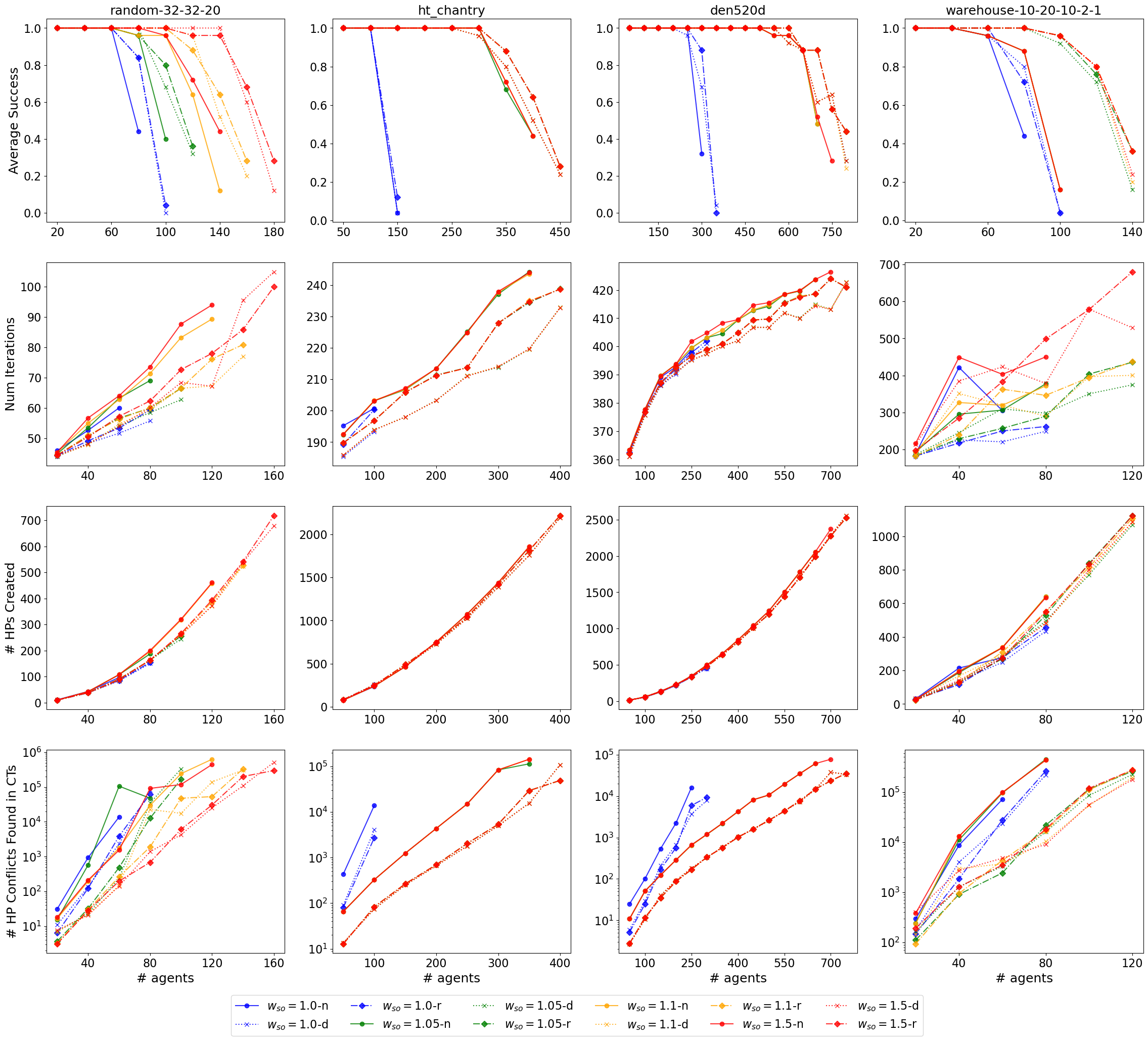
Figure A1: We plot statistics of SS-CBS with different high-level suboptimality (colored) and CT tie-breaking (line style).

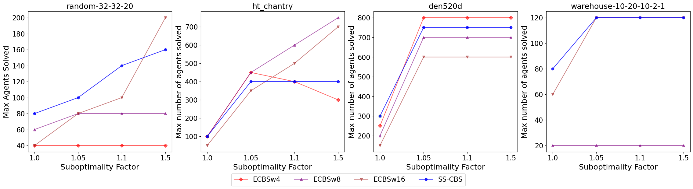
Figure A2: We compare the effects of increasing the high-level suboptimality factor on SS-CBS and windowed ECBS. The y-axis is the highest number of agents the method was able to solve at least 50% of the instances within the 1 minute timeout. ECBS with window $w=1,2$ failed on the lowest tried number of agents so only $w=4,8,16$ are plotted.

References

- Barer et al. (2014) Barer, M.; Sharon, G.; Stern, R.; and Felner, A. 2014. Suboptimal variants of the conflict-based search algorithm for the multi-agent pathfinding problem. In Seventh Annual Symposium on Combinatorial Search.
- Cardei and Du (2005) Cardei, M.; and Du, D. 2005. Improving Wireless Sensor Network Lifetime through Power Aware Organization. Wirel. Networks, 11(3): 333–340.
- Chan et al. (2024) Chan, S.-H.; Chen, Z.; Guo, T.; Zhang, H.; Zhang, Y.; Harabor, D.; Koenig, S.; Wu, C.; and Yu, J. 2024. The League of Robot Runners Competition: Goals, Designs, and Implementation. In ICAPS 2024 System’s Demonstration track.
- Erdmann and Lozano-Perez (1987) Erdmann, M.; and Lozano-Perez, T. 1987. On multiple moving objects. Algorithmica, 2(1): 477–521.
- Jiang et al. (2024) Jiang, H.; Zhang, Y.; Veerapaneni, R.; and Li, J. 2024. Scaling Lifelong Multi-Agent Path Finding to More Realistic Settings: Research Challenges and Opportunities. In Proceedings of the International Symposium on Combinatorial Search, volume 17, 234–242.
- Koenig and Likhachev (2006) Koenig, S.; and Likhachev, M. 2006. Real-time adaptive A*. In Nakashima, H.; Wellman, M. P.; Weiss, G.; and Stone, P., eds., 5th International Joint Conference on Autonomous Agents and Multiagent Systems (AAMAS 2006), Hakodate, Japan, May 8-12, 2006, 281–288. ACM.
- Koenig and Sun (2009) Koenig, S.; and Sun, X. 2009. Comparing real-time and incremental heuristic search for real-time situated agents. Autonomous Agents and Multi-Agent Systems, 18: 313–341.
- Korf (1990) Korf, R. E. 1990. Real-time heuristic search. Artificial Intelligence, 42(2): 189–211.
- Li et al. (2022) Li, J.; Chen, Z.; Harabor, D.; Stuckey, P. J.; and Koenig, S. 2022. MAPF-LNS2: Fast Repairing for Multi-Agent Path Finding via Large Neighborhood Search. Proceedings of the AAAI Conference on Artificial Intelligence, 36(9): 10256–10265.
- Li et al. (2021) Li, J.; Harabor, D.; Stuckey, P. J.; and Koenig, S. 2021. Pairwise Symmetry Reasoning for Multi-Agent Path Finding Search. CoRR, abs/2103.07116.
- Li, Ruml, and Koenig (2021) Li, J.; Ruml, W.; and Koenig, S. 2021. EECBS: A bounded-suboptimal search for multi-agent path finding. In Proceedings of the AAAI Conference on Artificial Intelligence (AAAI), 12353–12362.
- Li et al. (2020) Li, J.; Tinka, A.; Kiesel, S.; Durham, J. W.; Kumar, T. K. S.; and Koenig, S. 2020. Lifelong Multi-Agent Path Finding in Large-Scale Warehouses. In Proceedings of the 19th International Conference on Autonomous Agents and MultiAgent Systems, AAMAS ’20, 1898–1900. Richland, SC: International Foundation for Autonomous Agents and Multiagent Systems. ISBN 9781450375184.
- Okumura (2022) Okumura, K. 2022. LaCAM: Search-Based Algorithm for Quick Multi-Agent Pathfinding. arXiv:2211.13432.
- Okumura et al. (2022) Okumura, K.; Machida, M.; Défago, X.; and Tamura, Y. 2022. Priority inheritance with backtracking for iterative multi-agent path finding. Artificial Intelligence, 310: 103752.
- Rivera, Baier, and Hernandez (2013) Rivera, N.; Baier, J. A.; and Hernandez, C. 2013. Weighted real-time heuristic search. In Proceedings of the 2013 International Conference on Autonomous Agents and Multi-Agent Systems, AAMAS ’13, 579–586. Richland, SC: International Foundation for Autonomous Agents and Multiagent Systems. ISBN 9781450319935.
- Sharon et al. (2015) Sharon, G.; Stern, R.; Felner, A.; and Sturtevant, N. R. 2015. Conflict-based search for optimal multi-agent pathfinding. Artificial Intelligence, 219: 40–66.
- Sigurdson et al. (2018) Sigurdson, D.; Bulitko, V.; Yeoh, W.; Hernández, C.; and Koenig, S. 2018. Multi-Agent Pathfinding with Real-Time Heuristic Search. In 2018 IEEE Conference on Computational Intelligence and Games (CIG), 1–8.
- Silver (2005) Silver, D. 2005. Cooperative Pathfinding. In Proceedings of the First AAAI Conference on Artificial Intelligence and Interactive Digital Entertainment, AIIDE’05, 117–122. AAAI Press.
- Stern et al. (2019) Stern, R.; Sturtevant, N. R.; Felner, A.; Koenig, S.; Ma, H.; Walker, T. T.; Li, J.; Atzmon, D.; Cohen, L.; Kumar, T. K. S.; Boyarski, E.; and Bartak, R. 2019. Multi-Agent Pathfinding: Definitions, Variants, and Benchmarks. Symposium on Combinatorial Search (SoCS), 151–158.
- Veerapaneni, Kusnur, and Likhachev (2023) Veerapaneni, R.; Kusnur, T.; and Likhachev, M. 2023. Effective Integration of Weighted Cost-to-Go and Conflict Heuristic within Suboptimal CBS. In Thirty-Seventh AAAI Conference on Artificial Intelligence, AAAI 2023, Washington, DC, USA, February 7-14, 2023, 11691–11698. AAAI Press.
- Veerapaneni et al. (2024) Veerapaneni, R.; Wang, Q.; Ren, K.; Jakobsson, A.; Li, J.; and Likhachev, M. 2024. Improving Learnt Local MAPF Policies with Heuristic Search. International Conference on Automated Planning and Scheduling, 34(1): 597–606.
- Wagner and Choset (2011) Wagner, G.; and Choset, H. 2011. M*: A complete multirobot path planning algorithm with performance bounds. In 2011 IEEE/RSJ International Conference on Intelligent Robots and Systems, 3260–3267.
- Zhang et al. (2024) Zhang, Y.; Chen, Z.; Harabor, D.; Bodic, P. L.; and Stuckey, P. J. 2024. Planning and Execution in Multi-Agent Path Finding: Models and Algorithms. Proceedings of the International Conference on Automated Planning and Scheduling, 34(1): 707–715.