On the expressiveness and spectral bias of KANs
Abstract
Kolmogorov-Arnold Networks (KAN) [46] were very recently proposed as a potential alternative to the prevalent architectural backbone of many deep learning models, the multi-layer perceptron (MLP). KANs have seen success in various tasks of AI for science, with their empirical efficiency and accuracy demonstrated in function regression, PDE solving, and many more scientific problems.
In this article, we revisit the comparison of KANs and MLPs, with emphasis on a theoretical perspective. On the one hand, we compare the representation and approximation capabilities of KANs and MLPs. We establish that MLPs can be represented using KANs of a comparable size. This shows that the approximation and representation capabilities of KANs are at least as good as MLPs. Conversely, we show that KANs can be represented using MLPs, but that in this representation the number of parameters increases by a factor of the KAN grid size. This suggests that KANs with a large grid size may be more efficient than MLPs at approximating certain functions. On the other hand, from the perspective of learning and optimization, we study the spectral bias of KANs compared with MLPs. We demonstrate that KANs are less biased toward low frequencies than MLPs. We highlight that the multi-level learning feature specific to KANs, i.e. grid extension of splines, improves the learning process for high-frequency components. Detailed comparisons with different choices of depth, width, and grid sizes of KANs are made, shedding some light on how to choose the hyperparameters in practice.
1 Introduction
Recently, in [46], a novel architecture called Kolmogorov-Arnold Networks (KANs) was proposed as a potentially more accurate and interpretable alternative to standard multi-layer perceptron (MLP) [18, 29]. The KAN architecture leverages the Kolmogorov-Arnold representation theorem (KART) [35, 36] to parameterize functions. KANs share the same fully connected structures as MLPs, while putting learnable activation functions on edges as opposed to a fixed activation function on nodes for MLPs. B-splines are used to parameterize the learned nonlinearity and in practice one can go beyond the two-layer construction indicated by KART. KANs can be conceptualized as a hybrid of splines and MLPs, and the combination of compositional nonlinearity with 1D splines contributes to both the accuracy and interpretability of KANs.
In this article, we study the approximation theory and spectral bias of KANs and compare them with MLPs. Specifically, we show that any MLP with the ReLUk activation function can be reparameterized as a KAN with a comparable number of parameters. This establishes that the representation and approximation power of KANs is at least as great as that of MLPs. On the other hand, we also show that any KAN (without SiLU non-linearity) can be represented using an MLP. However, the number of parameters in the MLP representation is larger by a factor proportional to the grid size of the KAN. While we do not know if our construction is optimal, this suggests that KANs with a large grid size may be more efficient at parameterizing certain classes of functions than MLPs. We combine these results with existing optimal approximation rates for MLPs to obtain approximation rates for KANs on Sobolev spaces.
Next, we study the spectral bias phenomenon in the training of KANs. Standard MLPs with ReLU activations (or even tanh) are known to suffer from the spectral bias [53, 75, 76], in the sense that they will fit low-frequency components first. This is in contrast to traditional iterative numerical methods like the Jacobi method which learn high frequencies first [75]. Although the spectral bias acts as a regularizer which improves performance for machine learning applications [53, 84, 51, 87, 23], for scientific computing applications it may be necessary to learn high-frequencies as well. To alleviate the spectral bias, high-frequency information has to be encoded using methods like Fourier feature mapping [66, 69, 10, 49], or one needs to use nonlinear activation functions more similar to traditional methods; see for example the hat activation function [28] which resembles a finite element basis. We theoretically consider a single KAN layer and show that it does not suffer from the spectral bias by analyzing gradient descent for minimizing a least squares objective. Although our analysis is necessarily highly simplified, we argue that it provides some evidence and intuition showing that KANs will have a reduced spectral bias compared with MLPs.
Finally, we study the spectral bias of KANs experimentally on a wide variety of problems, including 1D frequency fitting, fitting samples from a higher-dimensional Gaussian kernel, and solving the Poisson equation with a high-frequency solutions. Based upon the results of our experiments, KANs consistently suffer less from the spectral bias. This also helps explain why KANs are more subject to noise and overfitting, as observed in [60], while grid coarsening (the opposite of grid extension) helps increase the spectral bias and reduces overfitting. Notice that the highest frequency that a single layer of KANs can learn is restricted to the number of grid points we use. The compositional structure associated with the depth also plays a role in learning the different frequencies. We study the effect of depths, widths, and grid sizes of KANs for the spectral bias, and draw conclusions about best practices when choosing KAN hyperparameters.
Our contribution.
Our goal in this paper is to theoretically compare the KAN architecture with the commonly used MLP architecture. Our specific contributions are as follows:
-
•
We compare the approximation and representation ability of KANs and MLPs. We show that KANs are at least as expressive as MLPs. We use this to obtain approximation rates for KANs on Sobolev spaces.
-
•
We theoretically analyze gradient descent applied to optimize the least squares loss using a single layer KAN. Based upon this analysis, we argue that KANs, unlike MLPs, do not suffer much from a spectral bias.
-
•
We provide numerical experiments demonstrating that KANs exhibit less of a spectral bias than MLPs on a variety of problems. This validates our theory and also provides a partial explanation for the success of KANs on problems in scientific computing.
2 Prior Work
A theory on the approximation ability of KANs in the function class of compositionally smooth functions was proposed as KAT in [46]. A convergence result independent of the dimension was obtained, leveraging the approximation theory of 1D splines. Compared with the universal approximation theorem of MLPs, KANs take advantage of the intrinsically low-dimensional compositional representation of underlying functions. This result shares an analogy to the rate in generalization error bounds of finite training samples, for a similar space studied for regression problems; see [30, 34], and also specifically for MLPs with ReLU activations [57]. On the other hand, for general Sobolev or Besov spaces, sharp approximation rates have been obtained for ReLU-MLPs (and more generally MLPs with most piecewise polynomial activation functions) [80, 8, 63]. These rates exhibit the curse of dimensionality, which is unavoidable due to the fact that Sobolev and Besov spaces with fixed smoothness are very large in high dimensions.
There are also subsequent works exploring other parametrizations of activation functions in the KAN formulation, including special polynomials [3, 58, 67], rational functions [4], radial basis function [41, 68], Fourier series [73], and wavelets [12, 59]. Active follow-up research focuses on applying KANs to various domains, such as partial differential equations [72, 62, 55] and operator learning [1, 62, 48], graphs [14, 19, 32, 85], time series [70, 25, 74, 24], computer vision [17, 6, 39, 16, 59, 11], and various scientific problems [43, 44, 77, 26, 37, 40, 5, 42, 50, 52]. In the KAN 2.0 paper [45], multiplication was introduced as a built-in modularity of KANs and the connection between KANs and scientific problems was further established in terms of identifying important features, modular structures, and symbolic formulas. In this article, we focus on the original B-spline formulation, one of the reasons being its alignment with continual learning and adaptive learning; see also [55].
The spectral bias of MLPs has been studied both experimentally and theoretically in a variety of works, see for instance [53, 84, 75, 76, 28, 51, 15, 9, 23, 86, 56] and the references therein. This phenomenon is proposed as explaining the regularizing effect of stochastic gradient descent [53, 23]. So far, the spectral bias of KANs has not been studied in detail, and it is this gap that we aim to close in this work.
3 Representation and Approximation
In this section, we study how to represent ReLUk MLPs using KANs with degree splines and vice-versa. Using this, we establish approximation rates for KANs from the corresponding results for MLPs.
3.1 Review of the KAN Architecture
We recall the following definitions of the Kolmogorov-Arnold Network (KAN) architecture introduced in [46]. We refer to [46] for a thorough treatment of all details mentioned here.
KAN architecture
The Kolmogorov-Arnold representation theorem (KART) states that any multivariate continuous function on a bounded domain can be represented as a finite composition of univariate continuous functions and addition. Specifically for a continuous , there exists continuous 1D functions such that (see for instance [13])
| (1) |
Inspired by KART corresponding to a two-layer neural network representation, the authors in [46] unified the inner and outer functions via the proposed KAN layers and generalized the idea of composition to arbitrary depths. A KAN can be represented by an integer array . Here is the number of layers and and are input and output dimensions respectively. denotes the number of neurons in the -th neuron layer. Usually, we choose as the width and refer to as the depth of the KAN. Layer maps a vector to , via nonlinear activations and additions, in the matrix form as
| (2) |
The overall network can be written as a composition of KAN layers as
| (3) |
Each activation function in (2) is parametrized by a linear combination of -th order B-splines and a SiLu nonlinearity. Namely
| (4) |
where is the grid size, are spline basis and , are trainable coefficients. The ranges of the grid points of the B-splines are updated on the fly, based on the range of the output of the previous layer. For on a bounded interval , consider the uniform grid , uniformally extended to . On this grid there are B-spline basis functions, with the B-spline being non-zero only on .
Grid extension
A very important structure of KANs proposed in [46] is the grid extension technique, inheriting the multi-level fine-graining from splines. One can first train KANs with fewer parameters to a desired accuracy, before making the spline grids finer with initialization from the coarser grid and continuing the training procedure. Grid extensions for all splines in a KAN can be performed independently and adaptively. We highlight that this technique is specific to the choice of splines as parameterizations of activation functions, and is particularly useful in the training process; see for example the discussion of spectral bias in the next section.
Approximation theory, KAT
We recollect the approximation theory established for compositionally smooth functions in [46].
Theorem 3.1.
Let . Suppose that a function admits a representation
| (5) |
as in (3), where each one of the is -times continuously differentiable. Then there exists a constant depending on and its representation, such that we have the following approximation bound in terms of the grid size : there exist -th order B-spline functions such that for any , we have the bound for the -norm
| (6) |
3.2 Reparametrization of KANs and MLPs
Next, we compare the approximation capabilities of KANs and MLPs. In particular, we have the following result showing that any ReLUk MLP can be exactly represented using a KAN with degree splines which is only slightly larger. We remark that this includes the case where , i.e. the popular and standard ReLU activation function.
Theorem 3.2.
Let be a bounded domain. Suppose that a function can be represented by an MLP with width , depth , and activation function for . Then there exists a KAN with width , depth at most , and grid size with -th order B-spline functions such that
| (7) |
for all .
On the other hand, we may ask whether every KAN can also be expressed using an MLP of a comparable size. If the functions in the KAN representation have weight in (3), then it is clear that we can not represent the resulting KAN using an MLP with activation , since the smooth function is not a polynomial. Essentially, the SiLU nonlinearity cannot be captured by a ReLUk MLP. However, if this nonlinearity is not present, then a KAN can be represented using a ReLUk MLP.
Theorem 3.3.
Suppose that a function can be represented by a KAN with width , depth , and grid size with -th order B-spline functions. Assume also that the weight in (3) for all of the activations appearing in the KAN. Then there exists an MLP with width , depth at most , and activation function which represents .
We remark that the width in this result scales like so that the number of parameters in the MLP scales like , while the number of parameters in the KAN scales like . This appears to indicate that KANs with a large number of breakpoints at each node may be more efficient in expressing certain functions than MLPs, although we don’t know whether the preceding theorem is sharp.
Using these results, we can draw conclusions about the approximation capabilities of KANs by leveraging existing results about MLPs (see for instance [7, 38, 33, 64, 65, 27, 47, 61, 81, 63, 79, 78]). For example, we have the following result giving optimal approximation rates for very deep KANs on Sobolev spaces (see for instance [2] for the background on Sobolev spaces).
Corollary 3.4.
Let be a bounded domain with smooth boundary, and be such that . This guarantees that the compact Sobolev embedding holds.
Let be a fixed width (depending upon the input dimension ). Then for any and any , there exists a KAN with width , depth , and grid size with -th order -spline functions such that
| (8) |
where is a constant independent of .
This result, which follows immediately from Theorem 3.2 and the approximation rates for ReLU (and more generally piecewise polynomial) neural networks derived in [63], shows that very deep KANs attain an exceptionally good approximation rate on Sobolev spaces. In particular, in terms of the number of parameters they attain an approximation rate of , while a classical (even non-linear) method of approximation can only attain a rate of [21]. This phenomenon, which is often called superconvergence [20], also occurs for very deep ReLUk networks. However, it comes at the cost of parameters which are not encodable using a fixed number of bits and thus is not practically realizable [82, 63].
4 Spectral Bias
In this section, we study the spectral bias of KANs and compare it to that of MLPs. The spectral bias, or frequency principle, refers to the observation that neural networks trained with gradient descent tend to be biased toward lower frequencies, i.e. that lower frequencies are learned first. This phenomenon has been well-documented and studied for MLPs, see for instance [53, 84, 75, 76, 28, 51, 15, 9, 23, 86], and it is our purpose here to develop an analogous theory for KANs. We remark that although the spectral bias is considered a form of regularization which is desirable for machine learning tasks [53, 84, 51, 87, 23], for scientific computing applications it is typically important to capture all frequencies and so the spectral bias may negatively affect the performance of neural networks for such applications [71, 54, 15, 28].
4.1 Spectral bias theory for shallow KANs
We consider the spectral bias properties of KANs with a single layer. This theory is very similar to the theory developed in [28, 86, 56] for the spectral bias of single hidden layer MLPs. The key observation is that a single layer KAN is a linear model. In particular, we see that if then the KAN applied to an input is (for simplicity, we consider the case of a KAN without the SiLu non-linearity)
| (9) |
where are the parameters of the KAN. Here where is the dimension of the output, , and . Note that the only parameter here is the grid size , since the width is determined by the input and output dimensions.
Based upon this, we can analyze least squares fitting with shallow KANs. In particular, let be the (symmetric) unit cube in , let be a target function we are trying to learn, and consider the (continuous) least squares regression loss
| (10) |
Due to the representation (9), this loss function is quadratic in the parameters . Let denote the corresponding Hessian matrix, i.e. so that
This Hessian matrix (indexed by ) is given by
| (11) |
The convergence of gradient descent on the least squares regression is determined by the eigendecomposition of the Hessian matrix which is estimated in the following theorem. The theorem is essentially a generalization of the fact that the Gram matrix of the B-spline basis is well conditioned (see for instance [22], Theorem 4.2 in Chapter 5).
Theorem 4.1.
Given a single hidden layer KAN with grid size , degree B-splines, input dimension and output dimension , let denote the Hessian matrix defined in (11) corresponding to the least squares fitting problem (10). Then the eigenvalues (here ) satisfy
| (12) |
for a constant depending only on the spline degree .
Theorem 4.1 shows that away from eigenvectors the matrix is well conditioned. This means that gradient descent will converge at the same rate in all directions orthogonal to these eigenvectors. Note that since the number of eigenvectors we must remove is independent of the grid size , we expect that when is relatively large most components of the KAN will converge at roughly the same rate toward the solution. Thus the KAN with a large number of grid points will not exhibit the same spectral bias toward low frequencies seen by MLPs. We remark that in constrast the Hessian associated with a two layer ReLU MLP with width has a condition number which scales like [28], which explains the strong spectral bias exhibited by ReLU MLPs.
Remark 4.2.
We note that the eigenvectors which must be excluded is not an artifact of the proof. In fact, this is due to the fact that the KAN parameterization is not unique. Indeed, the constant function can be parameterized in different ways by using the B-splines in each of the different directions. This ambiguity gives rise to directions in parameter space where the function parameterized by the KAN doesn’t change and this results in degenerate eigenvectors of the matrix .
The analysis given is necessarily highly simplified and heuristic. In particular, we only analyze a single layer of the KAN network and consider the continuous least squares loss. Nonetheless, we argue that it gives an explanation for why we would expect KANs to have a significantly different spectral bias than MLPs, and in particular why we expect that they learn all frequencies roughly similarly. In the remainder of this section, we experimentally test this hypothesis and compare the spectral bias of KANs with MLPs on a variety of simple problems. We implement these numerical experiments using the pykan package version .
4.2 1D waves of different frequencies
In the first example, we take the same setting as in [53] and study the regression of a linear combination of waves of different frequencies. Consider the function prescribed as
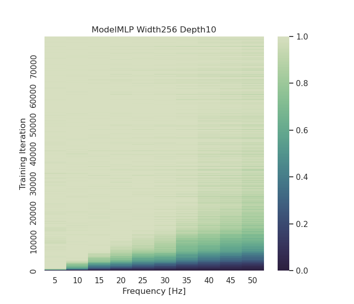
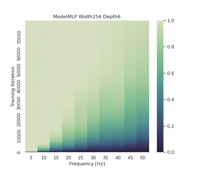
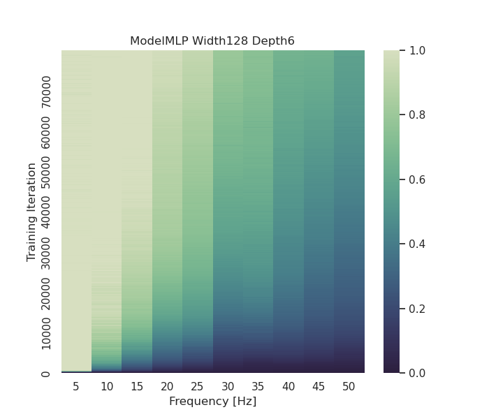
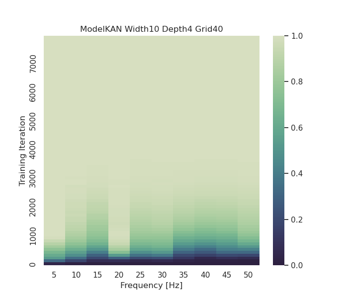
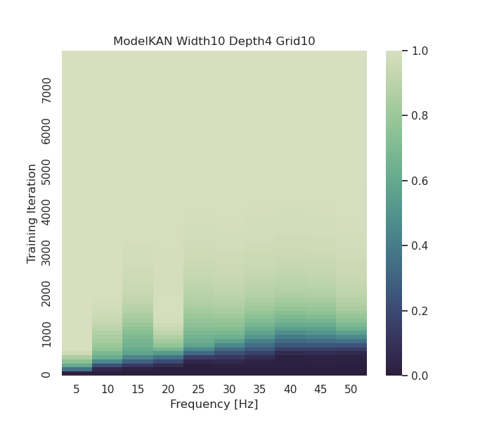
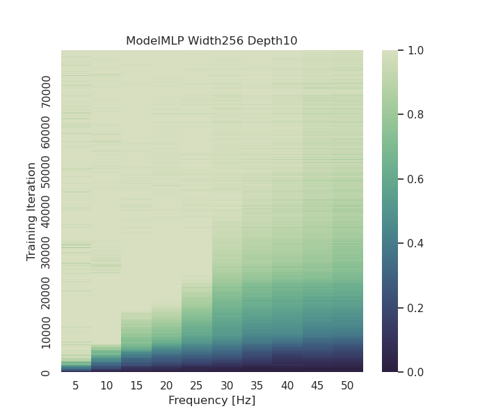
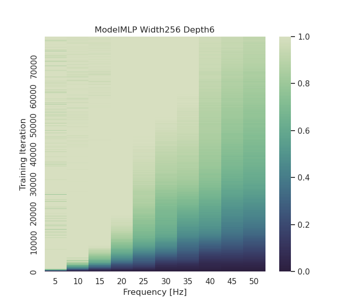
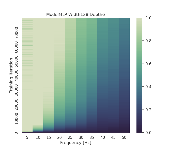
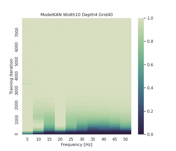
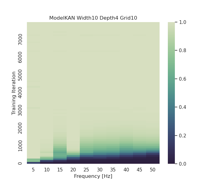
The phases are uniformly sampled from and we consider two cases of amplitudes: one with equal amplitude and another with increasing amplitude . We use a neural network, either ReLU MLP or KAN, to regress sampled at uniformly spaced points in , with full batch ADAM iteration as the optimizer with a learning rate of . For MLPs, we train with iterations as in [53]; for KANs, we only train with 8000 iterations. Normalized magnitudes of discrete Fourier transform at frequencies are computed as and averaged over 10 runs of different phases.
We plot the evolution of during training across all frequencies; see Figures 1, 2 for comparisons of MLPs and KANs with different sizes for equal and increasing amplitudes respectively. KANs suffer significantly less than MLPs from spectral biases. Once the size of KANs, especially the grid size and depth is large enough, KANs almost learn all frequencies at the same time, while even very deep and wide MLPs still have difficulties learning higher frequencies, even with x epochs!


4.3 Gaussian random field
In this example, we consider fitting functions sampled from a Gaussian random field. The target function is sampled from a -dimensional Gaussian random field with mean zero and covariance . Here small corresponds to rough functions and large corresponds to smooth functions.
To approximate the Gaussian random field, we sample using the KL expansion [31]. We sample points uniformly from and calculate the (empirical) covariance matrix . Then we truncate its first eigenpairs , with the cutoff threshold and sample approximately via
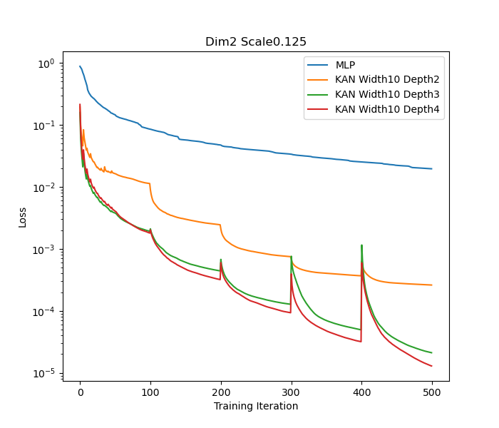
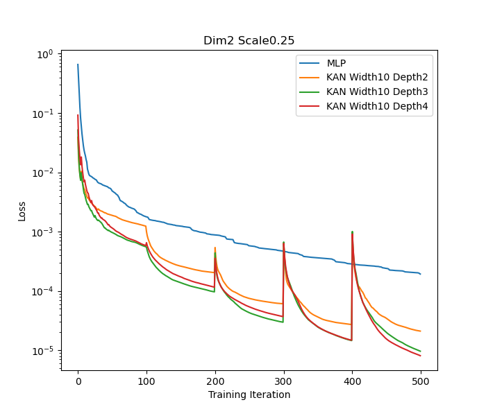
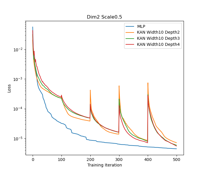
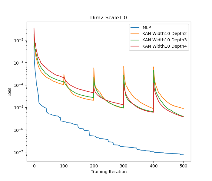
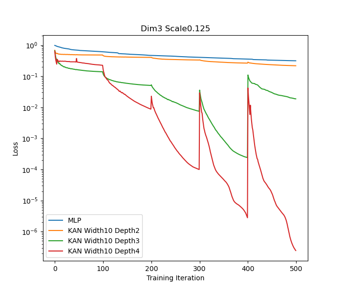
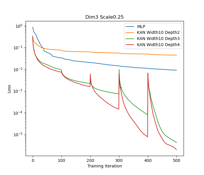
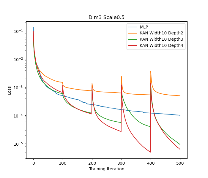
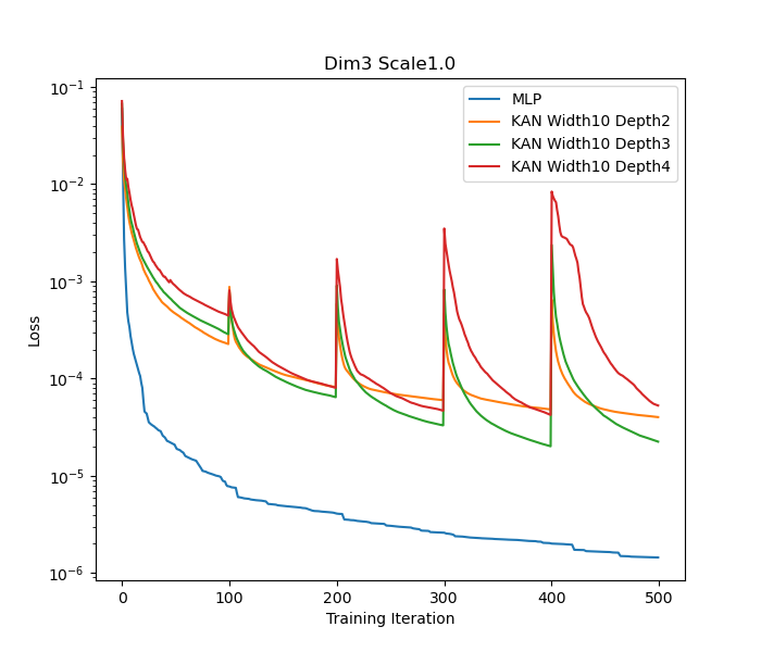
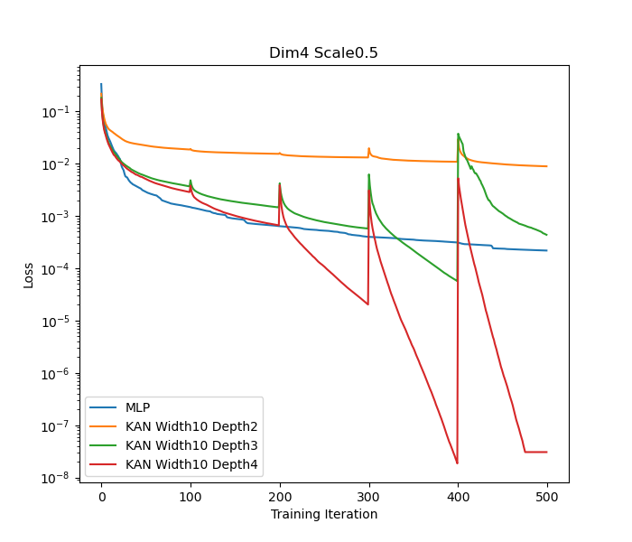
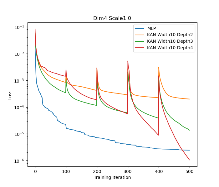
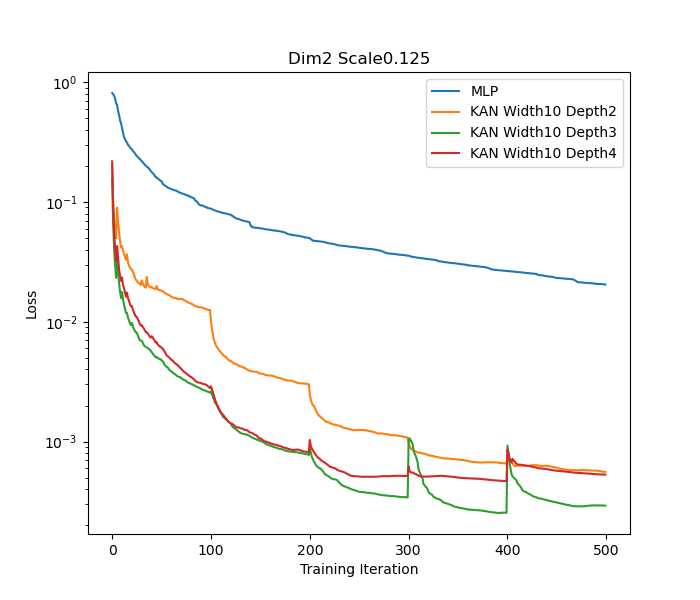
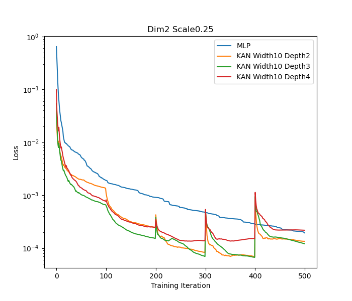
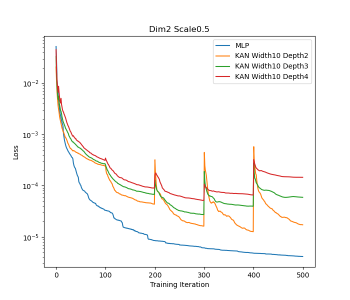
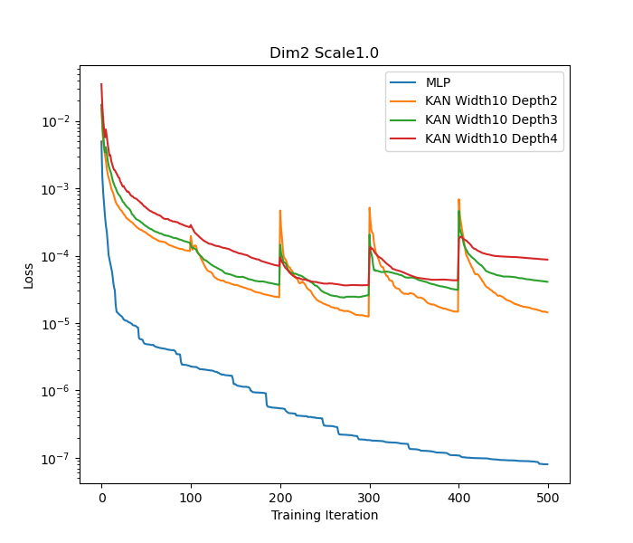
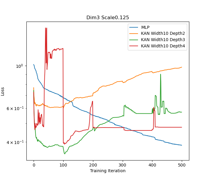
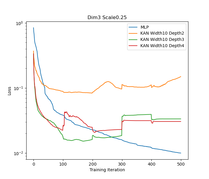
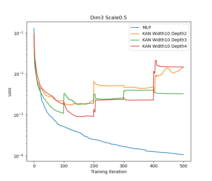
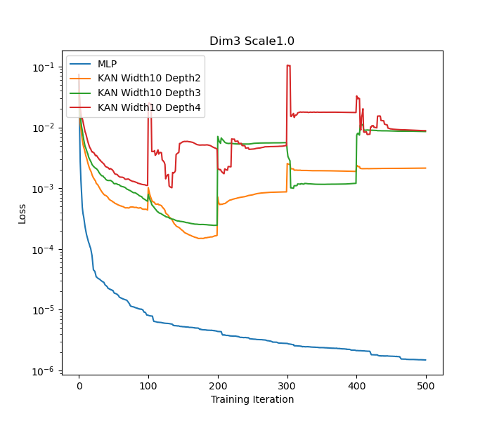
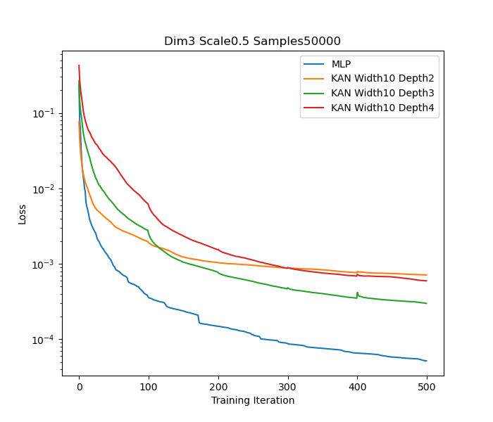
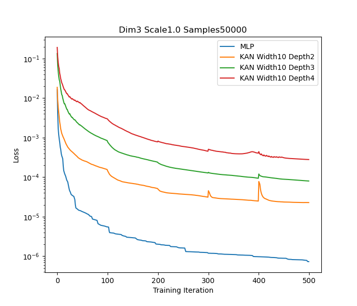
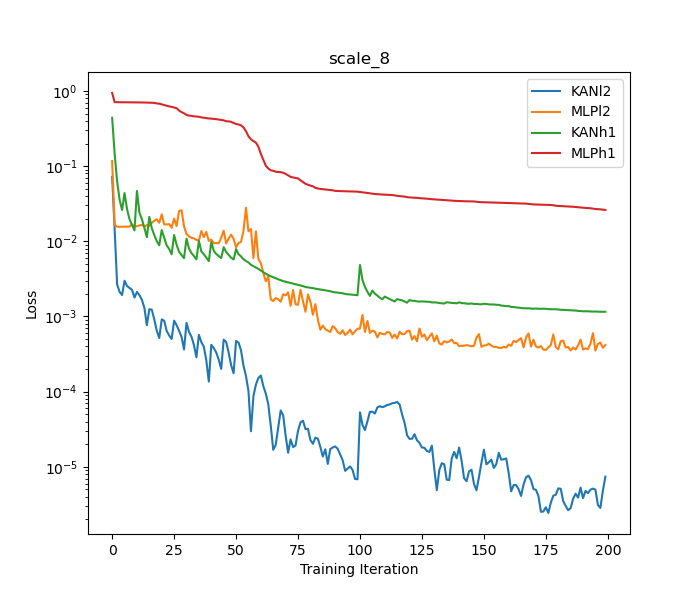
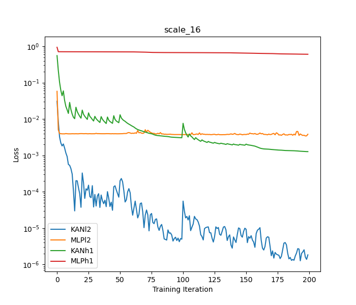
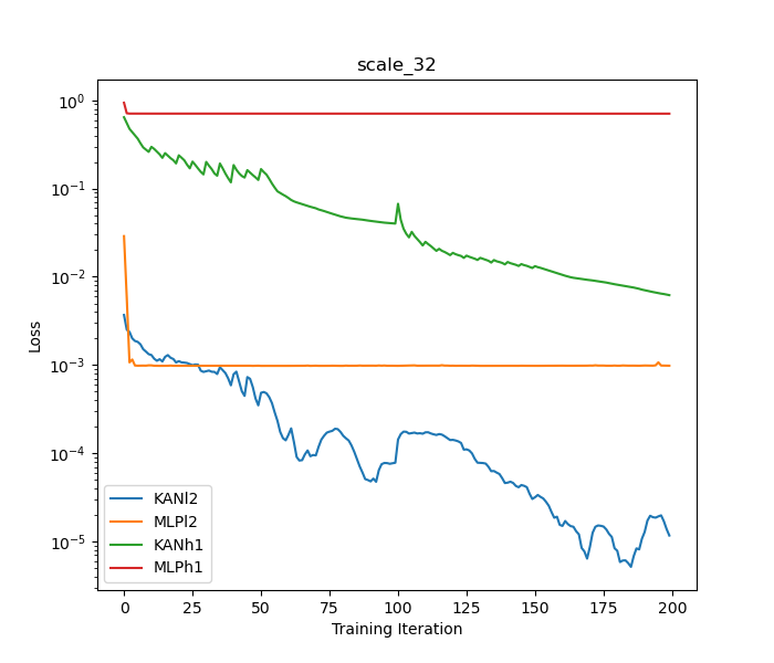
where are i.i.d standard Gaussians . For with different scales and dimensions , we split the points into training and testing points. We use MLPs and KANs with different sizes to regress on the training set, with the mean squared loss as the loss function. For MLPs, we use iterations of LBFGS iteration, and for KANs, we use the grid extension technique, with grid sizes , each trained with iterations of LBFGS.
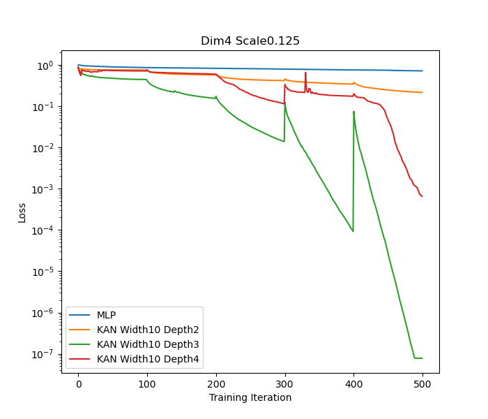
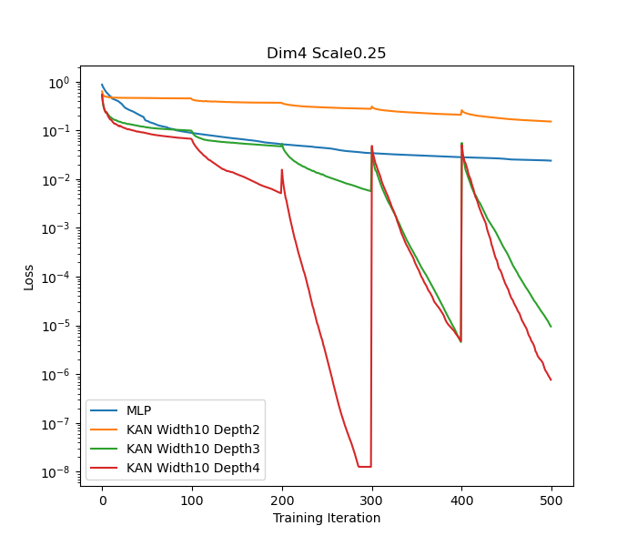
We plot the loss curves here and compare the losses of different scales and dimensions , using an MLP of layers and neurons in each hidden layer, and KANs with neurons in each hidden layer and layers; see Figure 3 for the regression loss on the training set with dimensions and scales , . We see that for larger scale and smoother functions, MLP performs better, while for smaller scale and rough functions, KANs perform better without suffering much from spectral biases, and grid extension is especially helpful. We remark that one can choose smaller grid sizes of KANs for smoother functions and obtain more accurate regressions.
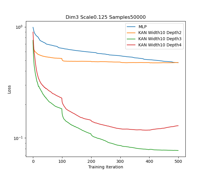
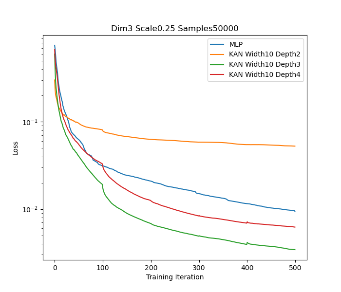
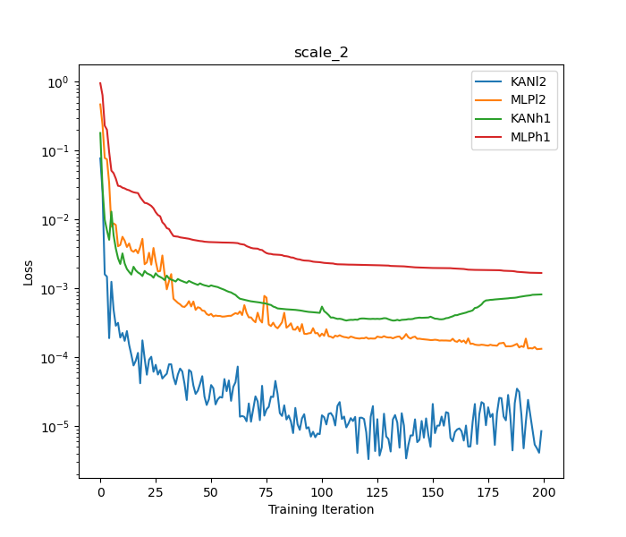
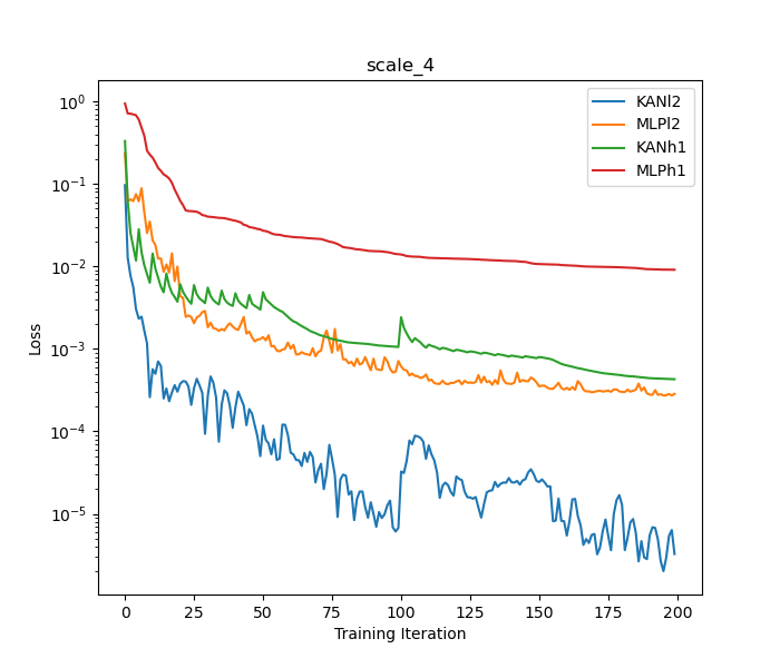
Precisely since KANs are not susceptible to spectral biases, they are likely to overfit to noises. As a consequence, we notice that KANs are more subject to overfitting on the training data regression when the task is very complicated; see the second line of Figure 4. On the other hand, we can increase the number of training points to alleviate the overfitting; see the last line of Figure 4 where we increased the number of training and test samples by x. We remark that the current implementation of grid extension is prone to oscillation after refining grids during the undersampled regime, as observed in [55], and we will improve it in future works.
4.4 PDE example
In this example, we solve the 1D Poisson equation with a high-frequency solution, similar to [75]. To be precise, consider the equation with zero Dirichlet boundary condition
| (13) |
Here for a frequency , the right-hand-side and the associated true solution are
The different frequencies are normalized in a way that for , the ground truth has the same energy () norm. We use the variational form of the elliptic equation and the associated Deep Ritz Method [83]. Parametrizing by a neural network, we minimize the loss
For frequencies , we use uniformly spaced sample points and the neural network using an MLP of 6 layers and 256 neurons in each hidden layer and a KAN of 2 layers with 10 neurons in the hidden layer. We choose the hyperparameter balancing the energy and boundary loss and perform LBFGS iterations. For MLPs, we use 200 iterations, and for KANs, we use grid sizes , each trained with 100 iterations. We plot the relative and losses compared to the ground truth in Figure 5. We can see that KANs perform consistently better, and the residue barely deteriorates when the frequency increases, whereas it becomes extremely hard for MLPs to optimize when
5 Concluding Remarks
In this work, we have compared the approximation and representation properties of KANs and MLPs. Based upon our theoretical and empirical analysis, we conclude that while KANs and MLPs are very similar from the perspective of approximation theory, i.e. the both parameterize similar classes of functions, they differ significantly in terms of their training dynamics. Specifically, KANs do not exhibit the same spectral bias toward low frequencies that MLPs do. Future work includes developing theory which can describe the training of deeper KANs, performing a more extensive experimental investigation of the spectral bias of KANs on more complicated problems, and investigating whether the reduced spectral bias of KANs improves their performance on scientific computing applications such as solving PDEs.
References
- [1] Diab W Abueidda, Panos Pantidis, and Mostafa E Mobasher. Deepokan: Deep operator network based on kolmogorov arnold networks for mechanics problems. arXiv preprint arXiv:2405.19143, 2024.
- [2] Robert A Adams and John JF Fournier. Sobolev spaces. Elsevier, 2003.
- [3] Alireza Afzal Aghaei. fkan: Fractional kolmogorov-arnold networks with trainable jacobi basis functions. arXiv preprint arXiv:2406.07456, 2024.
- [4] Alireza Afzal Aghaei. rkan: Rational kolmogorov-arnold networks. arXiv preprint arXiv:2406.14495, 2024.
- [5] Tashin Ahmed and Md Habibur Rahman Sifat. Graphkan: Graph kolmogorov arnold network for small molecule-protein interaction predictions. In ICML’24 Workshop ML for Life and Material Science: From Theory to Industry Applications, 2024.
- [6] Basim Azam and Naveed Akhtar. Suitability of kans for computer vision: A preliminary investigation. arXiv preprint arXiv:2406.09087, 2024.
- [7] Andrew R Barron. Universal approximation bounds for superpositions of a sigmoidal function. IEEE Transactions on Information theory, 39(3):930–945, 1993.
- [8] Peter L Bartlett, Nick Harvey, Christopher Liaw, and Abbas Mehrabian. Nearly-tight vc-dimension and pseudodimension bounds for piecewise linear neural networks. Journal of Machine Learning Research, 20(63):1–17, 2019.
- [9] Ronen Basri, Meirav Galun, Amnon Geifman, David Jacobs, Yoni Kasten, and Shira Kritchman. Frequency bias in neural networks for input of non-uniform density. In International conference on machine learning, pages 685–694. PMLR, 2020.
- [10] Nuri Benbarka, Timon Höfer, Andreas Zell, et al. Seeing implicit neural representations as fourier series. In Proceedings of the IEEE/CVF Winter Conference on Applications of Computer Vision, pages 2041–2050, 2022.
- [11] Alexander Dylan Bodner, Antonio Santiago Tepsich, Jack Natan Spolski, and Santiago Pourteau. Convolutional kolmogorov-arnold networks. arXiv preprint arXiv:2406.13155, 2024.
- [12] Zavareh Bozorgasl and Hao Chen. Wav-kan: Wavelet kolmogorov-arnold networks. arXiv preprint arXiv:2405.12832, 2024.
- [13] Jürgen Braun and Michael Griebel. On a constructive proof of kolmogorov’s superposition theorem. Constructive approximation, 30:653–675, 2009.
- [14] Roman Bresson, Giannis Nikolentzos, George Panagopoulos, Michail Chatzianastasis, Jun Pang, and Michalis Vazirgiannis. Kagnns: Kolmogorov-arnold networks meet graph learning. arXiv preprint arXiv:2406.18380, 2024.
- [15] Wei Cai and Zhi-Qin John Xu. Multi-scale deep neural networks for solving high dimensional pdes. arXiv preprint arXiv:1910.11710, 2019.
- [16] Minjong Cheon. Demonstrating the efficacy of kolmogorov-arnold networks in vision tasks. arXiv preprint arXiv:2406.14916, 2024.
- [17] Minjong Cheon. Kolmogorov-arnold network for satellite image classification in remote sensing. arXiv preprint arXiv:2406.00600, 2024.
- [18] George Cybenko. Approximation by superpositions of a sigmoidal function. Mathematics of control, signals and systems, 2(4):303–314, 1989.
- [19] Gianluca De Carlo, Andrea Mastropietro, and Aris Anagnostopoulos. Kolmogorov-arnold graph neural networks. arXiv preprint arXiv:2406.18354, 2024.
- [20] Ronald DeVore, Boris Hanin, and Guergana Petrova. Neural network approximation. Acta Numerica, 30:327–444, 2021.
- [21] Ronald A DeVore. Nonlinear approximation. Acta numerica, 7:51–150, 1998.
- [22] Ronald A DeVore and George G Lorentz. Constructive approximation. Grundlehren der mathematischen Wissenschaften, 1993.
- [23] Sara Fridovich-Keil, Raphael Gontijo Lopes, and Rebecca Roelofs. Spectral bias in practice: The role of function frequency in generalization. Advances in Neural Information Processing Systems, 35:7368–7382, 2022.
- [24] Remi Genet and Hugo Inzirillo. A temporal kolmogorov-arnold transformer for time series forecasting. arXiv preprint arXiv:2406.02486, 2024.
- [25] Remi Genet and Hugo Inzirillo. Tkan: Temporal kolmogorov-arnold networks. arXiv preprint arXiv:2405.07344, 2024.
- [26] Luis Fernando Herbozo Contreras, Jiashuo Cui, Leping Yu, Zhaojing Huang, Armin Nikpour, and Omid Kavehei. Kan-eeg: Towards replacing backbone-mlp for an effective seizure detection system. medRxiv, pages 2024–06, 2024.
- [27] Sean Hon and Haizhao Yang. Simultaneous neural network approximation for smooth functions. Neural Networks, 154:152–164, 2022.
- [28] Qingguo Hong, Jonathan W Siegel, Qinyang Tan, and Jinchao Xu. On the activation function dependence of the spectral bias of neural networks. arXiv preprint arXiv:2208.04924, 2022.
- [29] Kurt Hornik, Maxwell Stinchcombe, and Halbert White. Multilayer feedforward networks are universal approximators. Neural networks, 2(5):359–366, 1989.
- [30] Joel L Horowitz and Enno Mammen. Rate-optimal estimation for a general class of nonparametric regression models with unknown link functions. 2007.
- [31] Kari Karhunen. Under lineare methoden in der wahr scheinlichkeitsrechnung. Annales Academiae Scientiarun Fennicae Series A1: Mathematia Physica, 47, 1947.
- [32] Mehrdad Kiamari, Mohammad Kiamari, and Bhaskar Krishnamachari. Gkan: Graph kolmogorov-arnold networks. arXiv preprint arXiv:2406.06470, 2024.
- [33] Jason M Klusowski and Andrew R Barron. Approximation by combinations of ReLU and squared ReLU ridge functions with and controls. IEEE Transactions on Information Theory, 64(12):7649–7656, 2018.
- [34] Michael Kohler and Sophie Langer. On the rate of convergence of fully connected deep neural network regression estimates. The Annals of Statistics, 49(4):2231–2249, 2021.
- [35] A.N. Kolmogorov. On the representation of continuous functions of several variables as superpositions of continuous functions of a smaller number of variables. Dokl. Akad. Nauk, 108(2), 1956.
- [36] Andrei Nikolaevich Kolmogorov. On the representation of continuous functions of many variables by superposition of continuous functions of one variable and addition. In Doklady Akademii Nauk, volume 114, pages 953–956. Russian Academy of Sciences, 1957.
- [37] Akash Kundu, Aritra Sarkar, and Abhishek Sadhu. Kanqas: Kolmogorov arnold network for quantum architecture search. arXiv preprint arXiv:2406.17630, 2024.
- [38] Moshe Leshno, Vladimir Ya Lin, Allan Pinkus, and Shimon Schocken. Multilayer feedforward networks with a nonpolynomial activation function can approximate any function. Neural networks, 6(6):861–867, 1993.
- [39] Chenxin Li, Xinyu Liu, Wuyang Li, Cheng Wang, Hengyu Liu, and Yixuan Yuan. U-kan makes strong backbone for medical image segmentation and generation. arXiv preprint arXiv:2406.02918, 2024.
- [40] Xinhe Li, Zhuoying Feng, Yezeng Chen, Weichen Dai, Zixu He, Yi Zhou, and Shuhong Jiao. Coeff-kans: A paradigm to address the electrolyte field with kans. arXiv preprint arXiv:2407.20265, 2024.
- [41] Ziyao Li. Kolmogorov-arnold networks are radial basis function networks. arXiv preprint arXiv:2405.06721, 2024.
- [42] Hao Liu, Jin Lei, and Zhongzhou Ren. From complexity to clarity: Kolmogorov-arnold networks in nuclear binding energy prediction, 2024.
- [43] Mengxi Liu, Sizhen Bian, Bo Zhou, and Paul Lukowicz. ikan: Global incremental learning with kan for human activity recognition across heterogeneous datasets. arXiv preprint arXiv:2406.01646, 2024.
- [44] Mengxi Liu, Daniel Geißler, Dominique Nshimyimana, Sizhen Bian, Bo Zhou, and Paul Lukowicz. Initial investigation of kolmogorov-arnold networks (kans) as feature extractors for imu based human activity recognition. arXiv preprint arXiv:2406.11914, 2024.
- [45] Ziming Liu, Pingchuan Ma, Yixuan Wang, Wojciech Matusik, and Max Tegmark. Kan 2.0: Kolmogorov-arnold networks meet science. arXiv preprint arXiv:2408.10205, 2024.
- [46] Ziming Liu, Yixuan Wang, Sachin Vaidya, Fabian Ruehle, James Halverson, Marin Soljačić, Thomas Y Hou, and Max Tegmark. Kan: Kolmogorov-arnold networks. arXiv preprint arXiv:2404.19756, 2024.
- [47] Jianfeng Lu, Zuowei Shen, Haizhao Yang, and Shijun Zhang. Deep network approximation for smooth functions. SIAM Journal on Mathematical Analysis, 53(5):5465–5506, 2021.
- [48] George Nehma and Madhur Tiwari. Leveraging kans for enhanced deep koopman operator discovery. arXiv preprint arXiv:2406.02875, 2024.
- [49] Tiago Novello, Diana Aldana, and Luiz Velho. Taming the frequency factory of sinusoidal networks. arXiv preprint arXiv:2407.21121, 2024.
- [50] Yanhong Peng, Miao He, Fangchao Hu, Zebing Mao, Xia Huang, and Jun Ding. Predictive modeling of flexible ehd pumps using kolmogorov-arnold networks. arXiv preprint arXiv:2405.07488, 2024.
- [51] Tomaso Poggio, Kenji Kawaguchi, Qianli Liao, Brando Miranda, Lorenzo Rosasco, Xavier Boix, Jack Hidary, and Hrushikesh Mhaskar. Theory of deep learning iii: the non-overfitting puzzle. CBMM Memo, 73(1-38):2, 2018.
- [52] Pawel Pratyush, Callen Carrier, Suresh Pokharel, Hamid D Ismail, Meenal Chaudhari, and Dukka B KC. Calmphoskan: Prediction of general phosphorylation sites in proteins via fusion of codon aware embeddings with amino acid aware embeddings and wavelet-based kolmogorov arnold network. bioRxiv, pages 2024–07, 2024.
- [53] Nasim Rahaman, Aristide Baratin, Devansh Arpit, Felix Draxler, Min Lin, Fred Hamprecht, Yoshua Bengio, and Aaron Courville. On the spectral bias of neural networks. In International conference on machine learning, pages 5301–5310. PMLR, 2019.
- [54] Pratik Rathore, Weimu Lei, Zachary Frangella, Lu Lu, and Madeleine Udell. Challenges in training pinns: A loss landscape perspective. In Forty-first International Conference on Machine Learning, 2024.
- [55] Spyros Rigas, Michalis Papachristou, Theofilos Papadopoulos, Fotios Anagnostopoulos, and Georgios Alexandridis. Adaptive training of grid-dependent physics-informed kolmogorov-arnold networks. arXiv preprint arXiv:2407.17611, 2024.
- [56] Basri Ronen, David Jacobs, Yoni Kasten, and Shira Kritchman. The convergence rate of neural networks for learned functions of different frequencies. Advances in Neural Information Processing Systems, 32, 2019.
- [57] Johannes Schmidt-Hieber. Nonparametric regression using deep neural networks with relu activation function. 2020.
- [58] Seyd Teymoor Seydi. Exploring the potential of polynomial basis functions in kolmogorov-arnold networks: A comparative study of different groups of polynomials. arXiv preprint arXiv:2406.02583, 2024.
- [59] Seyd Teymoor Seydi. Unveiling the power of wavelets: A wavelet-based kolmogorov-arnold network for hyperspectral image classification. arXiv preprint arXiv:2406.07869, 2024.
- [60] Haoran Shen, Chen Zeng, Jiahui Wang, and Qiao Wang. Reduced effectiveness of kolmogorov-arnold networks on functions with noise. arXiv preprint arXiv:2407.14882, 2024.
- [61] Zuowei Shen, Haizhao Yang, and Shijun Zhang. Optimal approximation rate of ReLU networks in terms of width and depth. Journal de Mathématiques Pures et Appliquées, 157:101–135, 2022.
- [62] Khemraj Shukla, Juan Diego Toscano, Zhicheng Wang, Zongren Zou, and George Em Karniadakis. A comprehensive and fair comparison between mlp and kan representations for differential equations and operator networks. arXiv preprint arXiv:2406.02917, 2024.
- [63] Jonathan W Siegel. Optimal approximation rates for deep relu neural networks on Sobolev and Besov spaces. Journal of Machine Learning Research, 24(357):1–52, 2023.
- [64] Jonathan W Siegel and Jinchao Xu. Approximation rates for neural networks with general activation functions. Neural Networks, 128:313–321, 2020.
- [65] Jonathan W Siegel and Jinchao Xu. Sharp bounds on the approximation rates, metric entropy, and n-widths of shallow neural networks. Foundations of Computational Mathematics, pages 1–57, 2022.
- [66] Vincent Sitzmann, Julien Martel, Alexander Bergman, David Lindell, and Gordon Wetzstein. Implicit neural representations with periodic activation functions. Advances in neural information processing systems, 33:7462–7473, 2020.
- [67] Sidharth SS. Chebyshev polynomial-based kolmogorov-arnold networks: An efficient architecture for nonlinear function approximation. arXiv preprint arXiv:2405.07200, 2024.
- [68] Hoang-Thang Ta. Bsrbf-kan: A combination of b-splines and radial basic functions in kolmogorov-arnold networks. arXiv preprint arXiv:2406.11173, 2024.
- [69] Matthew Tancik, Pratul Srinivasan, Ben Mildenhall, Sara Fridovich-Keil, Nithin Raghavan, Utkarsh Singhal, Ravi Ramamoorthi, Jonathan Barron, and Ren Ng. Fourier features let networks learn high frequency functions in low dimensional domains. Advances in neural information processing systems, 33:7537–7547, 2020.
- [70] Cristian J Vaca-Rubio, Luis Blanco, Roberto Pereira, and Màrius Caus. Kolmogorov-arnold networks (kans) for time series analysis. arXiv preprint arXiv:2405.08790, 2024.
- [71] Sifan Wang, Xinling Yu, and Paris Perdikaris. When and why pinns fail to train: A neural tangent kernel perspective. Journal of Computational Physics, 449:110768, 2022.
- [72] Yizheng Wang, Jia Sun, Jinshuai Bai, Cosmin Anitescu, Mohammad Sadegh Eshaghi, Xiaoying Zhuang, Timon Rabczuk, and Yinghua Liu. Kolmogorov arnold informed neural network: A physics-informed deep learning framework for solving pdes based on kolmogorov arnold networks. arXiv preprint arXiv:2406.11045, 2024.
- [73] Jinfeng Xu, Zheyu Chen, Jinze Li, Shuo Yang, Wei Wang, Xiping Hu, and Edith C-H Ngai. Fourierkan-gcf: Fourier kolmogorov-arnold network–an effective and efficient feature transformation for graph collaborative filtering. arXiv preprint arXiv:2406.01034, 2024.
- [74] Kunpeng Xu, Lifei Chen, and Shengrui Wang. Kolmogorov-arnold networks for time series: Bridging predictive power and interpretability. arXiv preprint arXiv:2406.02496, 2024.
- [75] Zhi-Qin John Xu, Yaoyu Zhang, Tao Luo, Yanyang Xiao, and Zheng Ma. Frequency principle: Fourier analysis sheds light on deep neural networks. arXiv preprint arXiv:1901.06523, 2019.
- [76] Zhi-Qin John Xu, Yaoyu Zhang, and Yanyang Xiao. Training behavior of deep neural network in frequency domain. In Neural Information Processing: 26th International Conference, ICONIP 2019, Sydney, NSW, Australia, December 12–15, 2019, Proceedings, Part I 26, pages 264–274. Springer, 2019.
- [77] Shangshang Yang, Linrui Qin, and Xiaoshan Yu. Endowing interpretability for neural cognitive diagnosis by efficient kolmogorov-arnold networks. arXiv preprint arXiv:2405.14399, 2024.
- [78] Yahong Yang and Yulong Lu. Optimal deep neural network approximation for korobov functions with respect to sobolev norms. arXiv preprint arXiv:2311.04779, 2023.
- [79] Yahong Yang, Yue Wu, Haizhao Yang, and Yang Xiang. Nearly optimal approximation rates for deep super relu networks on sobolev spaces. arXiv preprint arXiv:2310.10766, 2023.
- [80] Dmitry Yarotsky. Error bounds for approximations with deep relu networks. Neural Networks, 94:103–114, 2017.
- [81] Dmitry Yarotsky. Optimal approximation of continuous functions by very deep ReLU networks. In Conference on Learning Theory, pages 639–649. PMLR, 2018.
- [82] Dmitry Yarotsky and Anton Zhevnerchuk. The phase diagram of approximation rates for deep neural networks. Advances in neural information processing systems, 33:13005–13015, 2020.
- [83] Bing Yu et al. The deep ritz method: a deep learning-based numerical algorithm for solving variational problems. Communications in Mathematics and Statistics, 6(1):1–12, 2018.
- [84] Chiyuan Zhang, Samy Bengio, Moritz Hardt, Benjamin Recht, and Oriol Vinyals. Understanding deep learning (still) requires rethinking generalization. Communications of the ACM, 64(3):107–115, 2021.
- [85] Fan Zhang and Xin Zhang. Graphkan: Enhancing feature extraction with graph kolmogorov arnold networks. arXiv preprint arXiv:2406.13597, 2024.
- [86] Shijun Zhang, Hongkai Zhao, Yimin Zhong, and Haomin Zhou. Why shallow networks struggle with approximating and learning high frequency: A numerical study. arXiv preprint arXiv:2306.17301, 2023.
- [87] Xiao Zhang, Haoyi Xiong, and Dongrui Wu. Rethink the connections among generalization, memorization and the spectral bias of dnns. arXiv preprint arXiv:2004.13954, 2020.
Appendix A Proofs
Proof of Theorem 3.2.
We will show that each layer of an MLP with the activation function can be represented by a KAN with two hidden layers, width and grid size with degree B-splines. By composing such layers, we obtain the desired result.
For a single layer of MLP, we consider the linear part and the non-linear activation separately. We first observe that on any compact subset of the linear function
| (14) |
can be represented with a single KAN layer of width by setting to the linear function
| (15) |
We claim that this linear function can be exactly represented on any interval in the form (4). To do this, we first set and choose the grid points for the B-splines to be
Note that based upon the KAN architecture, this corresponds to the extension of the uniform grid which has grid size . It is also easy to verify that there are B-splines supported on this grid, whose restriction to span the space of polynomials of degree . Thus, in particular, any linear function on can be represented as a linear combination of these B-splines.
Next, we consider the non-linear activation, which is given by the coordinatewise application of , i.e.
| (16) |
This can be represented by a single hidden layer KAN by setting
| (17) |
We claim that the functions can be represented in the form (4) on any finite interval . To to this, we again set and choose the grid points for the B-splines to be
This grid is the grid extension of the uniform grid which has grid size . It is easy also to verify that there are B-splines supported on this grid and that any piecewise polynomial on with a single breakpoint at which is is a linear combination of these B-splines. Hence the function can be represented on in the form (4) using this grid.
The proof is now completed by composing these layers and choosing sufficiently large so that for any input (which is bounded) the inputs and outputs of every neuron in the original MLP lie in the interval .
∎
Proof of Theorem 3.3.
The proof follows from the fact that each KAN activation function can be represented by a ReLUk neural network with one hidden layer of width . This is due to the fact that each is a linear combination of -splines (since we are assuming that in (4)). This implies that it must be a compactly support piecewise polynomial spline of degree whose -st derivative changes only on the extended grid which has points. We can now easily construct a shallow ReLUk network with one hidden node per grid point which matches the function . ∎
Proof of Theorem 4.1.
We first observe from (11) that the matrix is block diagonal with identical blocks. Denoting these blocks by , it thus suffices to prove that
| (18) |
To do this, we analyze the blocks and note that they take the form
| (19) |
Here the diagonal sub-blocks are the Gram matrix of the one-dimensional B-spline basis, i.e.
| (20) |
and the off-diagonal sub-blocks are rank one matrices
| (21) |
where the vector is given by
| (22) |
It is well-known that the Gram matrix is well-conditioned uniformly in for a fixed , i.e. for a fixed constant depending only upon . See for instance [22], Theorem 4.2 in Chapter 5, where it is shown that the -norm of a spline and the properly scaled -norm of its B-spline coefficients are equivalent up to a constant depending only on . This is equivalent to the well-conditioning of the Gram matrix .
In addition, we can easily verify using Jensen’s inequality (or Cauchy-Schwartz) that . Indeed, letting we see that
| (23) |
where the function .
Let be the vector of ones and note that
| (24) |
so that is a block diagonal matrix with diagonal blocks . We proceed to upper bound the largest eigenvalue of by
| (25) |
Writing with and and using that , we get the bound
| (26) |
Since we have which gives the bound
| (27) |
Next, we lower bound the -th eigenvalue of . For this, we use the Courant-Fisher minimax theorem to see that
| (28) |
where the maximum is taken over all subspaces of of codimension . We consider the specific subspace
| (29) |
and observe that for any with we have
| (30) |
while for the (which is orthogonal) we have
| (31) |
Thus, . Combining these bounds and using the well-conditioning of the Gram matrix , we get
| (32) |
for a constant which only depends upon . This completes the proof.
∎