Whole-Body Impedance Coordinative Control of Wheel-Legged Robot on Uncertain Terrain

Abstract

This article propose a whole-body impedance coordinative control framework for a wheel-legged humanoid robot to achieve adaptability on complex terrains while maintaining robot upper body stability. The framework contains a bi-level control strategy. The outer level is a variable damping impedance controller, which optimizes the damping parameters to ensure the stability of the upper body while holding an object. The inner level employs Whole-Body Control (WBC) optimization that integrates real-time terrain estimation based on wheel-foot position and force data. It generates motor torques while accounting for dynamic constraints, joint limits, friction cones, real-time terrain updates, and a model-free friction compensation strategy. The proposed whole-body coordinative control method has been tested on a recently developed quadruped humanoid robot. The results demonstrate that the proposed algorithm effectively controls the robot, maintaining upper body stability to successfully complete a water-carrying task while adapting to varying terrains.

I Introduction

Humanoid robots serve as a crucial platform for research in embodied intelligence, combining dexterous manipulation, agile locomotion, and artificial intelligence, and they will play an increasingly important role in people’s daily lives. Robots needs to adapt to uncertain terrain conditions, including varied ground materials like cobblestone and uphill or downhill slopes, while also maintaining passive stability in upper body tasks. This passive stability allows the robot to remain steady by passively responding to dynamic external forces, crucially enabling it to handle tasks involving delicate balance and object stability.

Achieving stability under unpredictable conditions is essential for robot applications in real-world environments, where the terrain and external forces may vary significantly. This adaptability is particularly critical for robots designed to navigate mixed terrain while carrying objects that require careful stability, such as trays with liquids or delicate equipment. At present, most of the bipedal or two wheel humanoid robots need to design complex control algorithms to maintain their own balance, and their load-bearing capacity is limited. Therefore, it is necessary to redefine the robot’s mechanical structure in the human-centered environment. These research directions are not systematic enough at present, so it is necessary to conduct research on these issues.

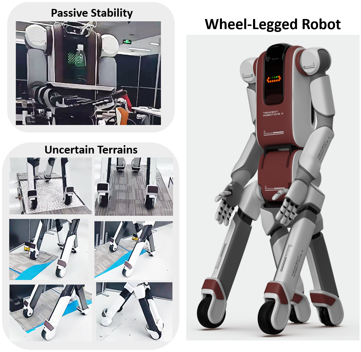
Figure 1: The newly developed wheel-legged robot, X-Man, with its 80 kg mass, introduces significant inertial challenges. Despite this, our work enables it to achieve upper-limb passive stability and demonstrate adaptability across varied uncertain terrains while maintaining balance.

In this paper, we present a novel whole-body control framework for our self-developed robot, X-Man. The main contributions are summarized as follows:

• The impedance coordinative controller is proposed to achieve passive stability and terrain adaption.

• A novel whole-body control of a humanoid robot is proposed, including whole-body dynamics optimization, terrain frame estimation and model-free compensation.

• Experiment validation on the X-man, demonstrated the capability of whole body motion control, complex terrain adaptability.

The remainder of this paper is organized as follows: Section II reviews related work. Section III details the robot system. The impedance coordinative controller and WBC controller are presented in Section IV, V, respectively. Section VI provides experiments. Section VII concludes the paper.

II Related Work

II-A The Humanoid Robot

Currently, there are three main types of humanoid robots, namely bipedal, two-wheel type, and quadrupedal [1]. Typical representatives of bipedal humanoid robots include Altas, TORO [2, 3]. Even the simplest movement of standing up requires a lot of energy for a bipedal robot. For two-wheeled humanoid robots, such as $\text{EVE}^{\text{R3}}$ [4]. This type of robot is mainly used on regular roads. For quadruped humanoid robots, such as Centauro and GITAI [5, 6]. This type of robot is mainly used in complex scenes, but due to its large weight, the overall dynamic performance and environmental adaptability are poor. In terms of usage, current humanoid robots are mainly used in outdoor and even space environment exploration [7].

In summary, there is currently little research on the exploration of robot morphology in human-centered environment. The robot form in such scenarios needs to be redefined.

II-B The Whole Body Control

The whole-body controller can be divided into least-square(LS) based solver and Quadratic Programming(QP) controller based solver [8]. As for the LS solution, the inverse dynamics based WBC of floating base robot with contact constraints was studied [9]. The divergent component of motion(also known as instantaneous capture point) and passive based whole body controller is utilized to achieve dynamic walking and even dynamic multi-contact transitions tasks for TORO [3]. And the QP-based optimization frame can be divided into two types as weighted quadratic programming(WQP) and hierarchical quadratic programming(HQP) [10]. The hierarchical optimization is also utilized to achieve perception-less terrain adaptation for ANYmal [11]. WBC is also utilizded to tracking the commanded COM (Center of mass) trajectories generated via 3D SLIP(spring loaded inverted pendulum) [12].

Besides, for robots with large inertia, the nonlinear characteristics of the robot joints are obvious [13]. At present, there is no systematic research on the WBC of large-inertia humanoid robots.

II-C The Impedance Control

The combination of impedance control and whole body control can achieve the whole body complaince. The Cartesian impedance control of robots has also been studied from a multi-priority perspective, including solutions based on Jacobi pseudo-inverse [14] and solutions solved by QP solver [15]. The impedance control and the optimization-based whole-body control framework is implemented to achieve stable biped walking [16]. And the optimal impedance planning by given the Cartesian inertia and computes the stiffness and damping gains without relying on force/torque sensor is also studied [17].

As for humanoid robots, there will be two impedance controllers in the same direction. Force control in this impedance-coupled situation in humanoid robots has rarely been studied before.

III Hardware and System Overview of X-Man

III-A Hardware Design

This paper aims to design a humanoid quadruped robot for human-centered environment. Common bipedal humanoid robots require a lot of energy and the design of complex control algorithms to achieve robot locomotion, and the system has poor robustness and weak anti-disturbance capabilities. In a human-centered environment, the robot need to gurantee terrain adaptability, and stable upper body manipulation capabilities. The robot adopts a wheel-leg composite design, which can greatly expand the range of movement and enhance movement stability, while still retaining the characteristics of a legged robot. The robot’s lower body joints, including the waist, hip, leg, and foot joints, are equipped with joint torque sensors. The upper body arms are covered with tactile skin. In addition, we define the head orientation as the front, and according to the configuration characteristics of the robot, it can be divided into front legs and hind legs, front wheels and rear wheels, front hip and rear hip.

III-B Control System Overview

III-B1 Control Objective

We derive the X-man controller with control objectives divided into two main components: (A) upper-body control, which includes passively stabilizing the upper limbs and minimizing the energy consumption of the lower limbs due to body oscillation; and (B) whole-body control(WBC), which involves tracking a desired trajectory.

For (A), the energy expenditure resulting from the force provided by the lower body to the upper body is computed by integrating the mechanical power $\rho_{1}(t)$ over a full cycle $T$. To maintain the stability of the upper limbs during holding an object, a stability term $\rho_{2}(t)$ is introduced. Thus, the total mechanical work associated with upper limb is expressed as:

$$E_{k}=\int_{0}^{T}\rho_{k}(t)\,dt.\ \ \ k=1,2$$ (1)

The decision variable for upper limb is the variable damping parameter.

For (B), whole-body control aims to achieve accurate trajectory tracking by applying joint torques. The objective function for WBC consists of a state regularization term combined with a body vibration suppression term to ensure stability and precise movement throughout the trajectory.

III-B2 Our Control Strategy

To achieve both control objectives above, we decompose our control strategy into outer and inner loops based on the platform’s architecture. The outer-loop control is to optimize and generate optimal damping parameters. The inner-loop control, which demands a much higher control frequency, uses WBC to generate the control torques based on estimated terrain information and updated trajectory from the outer loop. The overall X-Man control framework, illustrated in Fig. 3, consists of five main components: the desired trajectory generation part; the outer-loop impedance control part; the inner-loop WBC part; the joint torque tracking part; and the general momentum observation part.

It is worth mentioning that since X-Man has two coupled impedance controllers in the same direction, an impedance coordinative approach is adopted to achieve the optimization goal set in the previous section [18]. Joint force tracking is employed to monitor and regulate the driving torques for each joint, as computed by the WBC framework.

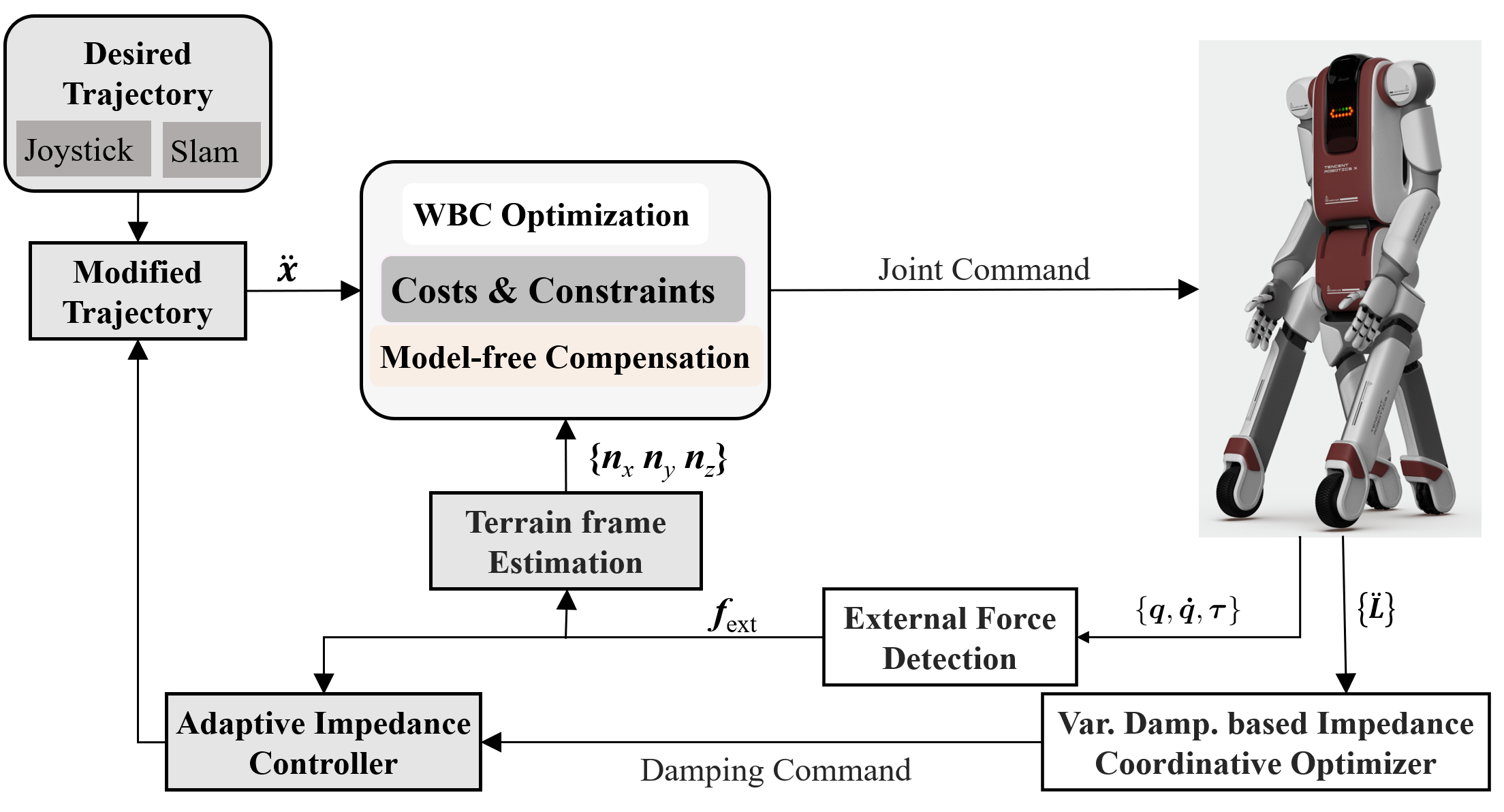
Figure 3: The overview controller framework of X-Man. Denote $\boldsymbol{q}$ and $\boldsymbol{x}$ are the joint value and point state of robot. $\boldsymbol{\dot{q}},\boldsymbol{\ddot{q}}$ are the angular velocity and acceleration. $\boldsymbol{\tau}$ is joint torque. $\{\boldsymbol{n}_{x},\boldsymbol{n}_{y},\boldsymbol{n}_{z}\}$ is the terrain frame. And $\boldsymbol{n}_{z}$ is unit normal vector, and $\boldsymbol{\boldsymbol{n}}_{x},\boldsymbol{n}_{y}$ are two orthonormal tangent vectors described with respect to the object frame.

IV Impedance Coordinative Controller

IV-A General Impedance Control

The closed-loop impedance control model is governed as:

$$\boldsymbol{M}\Delta\boldsymbol{\ddot{x}}+\boldsymbol{D}\Delta\boldsymbol{\dot{x}}+\boldsymbol{K}\Delta\boldsymbol{x}=\boldsymbol{F}_{e}$$ (2)

where $\boldsymbol{M}$, $\boldsymbol{D}$ and $\boldsymbol{K}$ represent the inertia, damping, and stiffness matrices, respectively. The term $\boldsymbol{F}_{e}$ denotes the external force corresponding to the displacement $\boldsymbol{x}$, where $\boldsymbol{x}$ represents a specific state of robot. Denote $\boldsymbol{x}^{{}^{\prime}}_{\text{ref}}(t)$ the reference value. $\Delta\boldsymbol{x}=\boldsymbol{x}(t)-\boldsymbol{x}^{{}^{\prime}}_{\text{ref}}(t)$ denotes the position error. Then, the modified reference acceleration $\boldsymbol{\ddot{x}}_{\text{ref}}$ is derived as:

$$\boldsymbol{\ddot{x}}=\boldsymbol{\ddot{x}}^{{}^{\prime}}_{\text{ref}}+\boldsymbol{M}^{-1}\left(\boldsymbol{F}_{e}-\boldsymbol{D}\Delta\boldsymbol{\dot{x}}-\boldsymbol{K}\Delta\boldsymbol{x}\right).$$ (3)

By integrating $\boldsymbol{\ddot{x}}$, the corresponding updated reference velocity $\boldsymbol{\dot{x}}_{\text{ref}}$ and updated reference position $\boldsymbol{x}_{\text{ref}}$ can be obtained. The updated reference values are utilized in the WBC controller.

The locomotion-related impedance control point can be set at either the base frame ($\Sigma_{B}$) or the Center of mass frame ($\Sigma_{O}$). Accordingly, the external force must first be transformed to the chosen reference point. Denote $\boldsymbol{f}_{\text{ext}}=[\boldsymbol{f}^{T}_{M}\ \boldsymbol{f}^{T}_{C}]^{T}\in\mathbb{R}^{(N_{D}N_{C})}$ the external force. $\boldsymbol{f}_{M}$ is the force for object manipulation. $\boldsymbol{f}_{C}$ is the ground contact force. $N_{C}$ is the number of contact point. $N_{D}$ is the dimension of contact force. For example, consider the case where the control point is set at $\Sigma_{B}$, the base wrench ${\boldsymbol{\hat{F}}}_{e,C}$ can be derived as:

$${\boldsymbol{\hat{F}}}_{e}=\sum{\boldsymbol{J}^{T}_{B,M,i}}\boldsymbol{S}_{M,i}{\boldsymbol{\hat{f}}}_{\text{ext}}+\sum{\boldsymbol{J}^{T}_{B,C,i}}\boldsymbol{S}_{C,i}{\boldsymbol{\hat{f}}}_{\text{ext}}$$ (4)

where $\boldsymbol{S}_{M,i},\boldsymbol{S}_{C,i}$ denote the section matrix for the $i$-th limb, and $\boldsymbol{S}_{M,i}{\boldsymbol{\hat{f}}}_{\text{ext}}={\boldsymbol{\hat{f}}}_{M}$, $\boldsymbol{S}_{C,i}{\boldsymbol{\hat{f}}}_{\text{ext}}={\boldsymbol{\hat{f}}}_{C}$, ${\boldsymbol{J}_{B,M,i}}$ denotes the contact Jacobian matrix for the $i$-th limb for the manipulation task, ${\boldsymbol{J}_{B,C,i}}$ denotes the contact Jacobian matrix for the $i$-th limb for the locomotion task. $\Sigma_{B}$ or $\Sigma_{O}$ will actively adjust its pose according to external forces. ${\boldsymbol{\hat{f}}}_{\text{ext}}$ can be obtained by the general momentum observer [19, 20].

IV-B Impedance Coordinative Control

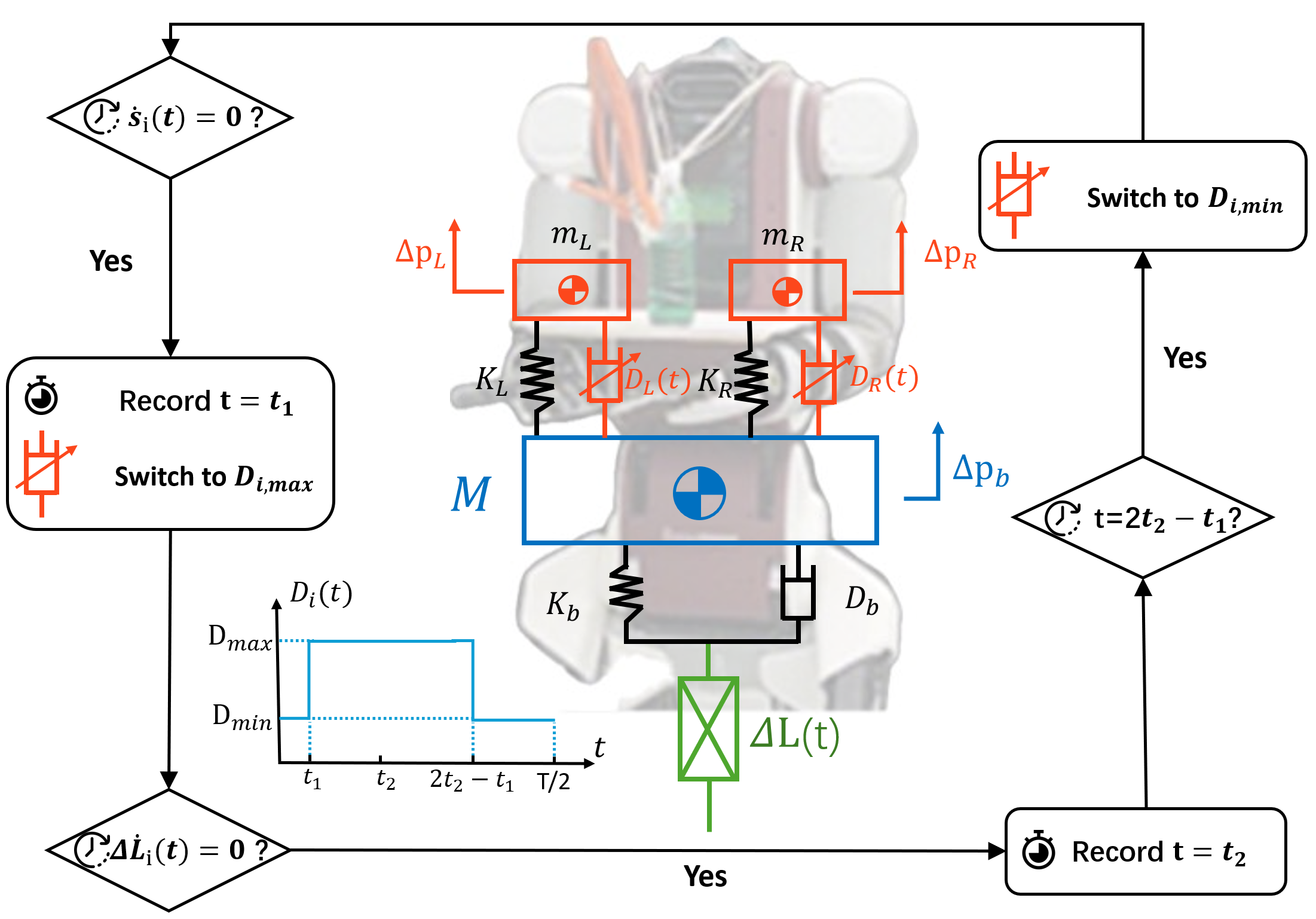
Figure 4: The dual-arm variable damping-based impedance coordinative controller, where $t_{1}$ represents the instant of zero relative motion between the load and the robot body, and $t_{2}$ is the instant when the variation in robot leg length reaches a steady state. The coefficients $\boldsymbol{K}_{b}$, $\boldsymbol{K}_{L}$, and $\boldsymbol{K}_{R}$ are the stiffness matrices, and $\boldsymbol{D}_{b}$, $\boldsymbol{D}_{L}$, and $\boldsymbol{D}_{R}$ are the damping matrices. These matrices are diagonal, representing stiffness and damping properties in the $x$, $y$, and $z$ directions for the body and loads. $M$ represents the body mass, while $m_{L}$ and $m_{R}$ represent the masses of the left and right loads. And $m_{L}$, $m_{R}$, and $M$ are the components in $\boldsymbol{M}$ of (2).

To maintain upper body stability during locomotion tasks in a large inertia robot, we treat the upper arms as a coupled dynamic system. Inspired by the suspended backpack principle [21], the dual arms are modeled as spring-variable damping mechanisms designed for lower limb energy saving and upper limbs passive stability. Passive stability allows the robot to keep an object stable, such as a tray, steady by naturally responding to dynamic external forces rather than actively adjusting its position.

IV-B1 Equality constraint of ICC

According to the mechanical structure of the X-man, we simplify the robot body as a mass block with a variable damper-spring mechanism connected to the left and right loads, and with an additional spring-damper mechanism below connecting with the robot legs, as shown Fig 4. We can then derive the dynamics equations of the body center of mass (CoM) and the loads.

$$M\Delta\ddot{\boldsymbol{p}}_{b}+(\boldsymbol{D}_{L}+\boldsymbol{D}_{L}+\boldsymbol{D}_{R})\Delta\dot{\boldsymbol{p}}_{b}+(\boldsymbol{K}_{b}+\boldsymbol{K}_{L}+\boldsymbol{K}_{R})\Delta\boldsymbol{p}_{b}=$$ (5)

$$\boldsymbol{K}_{b}\Delta\boldsymbol{L}+\boldsymbol{D}_{b}\Delta\dot{\boldsymbol{L}}+\begin{bmatrix}\boldsymbol{D}_{L}&\boldsymbol{D}_{R}\end{bmatrix}\begin{bmatrix}\Delta\dot{\boldsymbol{p}}_{L}\\ \Delta\dot{\boldsymbol{p}}_{R}\end{bmatrix}+\begin{bmatrix}\boldsymbol{K}_{L}&\boldsymbol{K}_{R}\end{bmatrix}\begin{bmatrix}\Delta\boldsymbol{p}_{L}\\ \Delta\boldsymbol{p}_{R}\end{bmatrix}$$

$$\begin{bmatrix}m_{L}&0\\ 0&m_{R}\end{bmatrix}\begin{bmatrix}\Delta\ddot{\boldsymbol{p}}_{L}\\ \Delta\ddot{\boldsymbol{p}}_{R}\end{bmatrix}+\begin{bmatrix}\boldsymbol{D}_{L}&0\\ 0&\boldsymbol{D}_{R}\end{bmatrix}\begin{bmatrix}\Delta\dot{\boldsymbol{p}}_{L}\\ \Delta\dot{\boldsymbol{p}}_{R}\end{bmatrix}+\begin{bmatrix}\boldsymbol{K}_{L}&0\\ 0&\boldsymbol{K}_{R}\end{bmatrix}\begin{bmatrix}\Delta\boldsymbol{p}_{L}\\ \Delta\boldsymbol{p}_{R}\end{bmatrix}$$ (6)

$$=\begin{bmatrix}\boldsymbol{D}_{L}&0\\ 0&\boldsymbol{D}_{R}\end{bmatrix}\begin{bmatrix}\Delta\dot{\boldsymbol{p}}_{b}\\ \Delta\dot{\boldsymbol{p}}_{b}\end{bmatrix}+\begin{bmatrix}\boldsymbol{K}_{L}&0\\ 0&\boldsymbol{K}_{R}\end{bmatrix}\begin{bmatrix}\Delta\boldsymbol{p}_{b}\\ \Delta\boldsymbol{p}_{b}\end{bmatrix}$$

Here, $\Delta\boldsymbol{p}_{b}=[\Delta p_{b_{x}},\Delta p_{b_{y}},\Delta p_{b_{z}}]^{T}$ represents the variation in the position of the body CoM in the $x$, $y$, and $z$ directions, while $\Delta\boldsymbol{p}_{L}=[\Delta p_{L_{x}},\Delta p_{L_{y}},\Delta p_{L_{z}}]^{T}$ and $\Delta\boldsymbol{p}_{R}=[\Delta p_{R_{x}},\Delta p_{R_{y}},\Delta p_{R_{z}}]^{T}$ denote the variations in the positions of the left and right loads, respectively. Other notations are defined in Fig. 4 and elaborated in the following two remarks.

Remark 1.

The values of $m_{L}$ and $m_{R}$ are determined based on the gravity measured by the tactile skin in a static state. These loads can either represent two different objects held by the left and right upper limbs or a single object with its weight distributed between both limbs.

Remark 2.

The function $\Delta\ddot{\boldsymbol{L}}(t)\in\mathbb{R}^{3}$ is determined by leg-hip motion, which can be pre-defined through motion planning and measured in real time using IMU sensors. Note that $\Delta\boldsymbol{L}(t)$ represents the variation in leg length during motion, not the absolute leg length. $\Delta\boldsymbol{L}(t)$ will directly determine the movement of the robot base and indirectly cause the change of the robot’s Center of mass. Moreover, $\Delta\boldsymbol{L}(t)$ arises as a response to dynamic external contact forces acting on the lower limbs. These contact forces introduce oscillations that propagate through the robot’s structure, necessitating passive stability to mitigate any impact on upper body.

By defining the relative displacements as $\boldsymbol{s_{b}}=\Delta\boldsymbol{p}_{b}-\Delta\boldsymbol{L}$, $\boldsymbol{s_{L}}=\Delta\boldsymbol{p}_{L}-\Delta\boldsymbol{p}_{b}$, $\boldsymbol{s_{R}}=\Delta\boldsymbol{p}_{R}-\Delta\boldsymbol{p}_{b}$, the system equations can be reformulated. Let the state vector be defined as:

$$\boldsymbol{x_{s}}=\begin{bmatrix}\boldsymbol{s_{b}}&\dot{\boldsymbol{s}}_{b}&\boldsymbol{s_{L}}&\dot{\boldsymbol{s}}_{L}&\boldsymbol{s_{R}}&\dot{\boldsymbol{s}}_{R}\end{bmatrix}^{T},$$

then the system dynamics can be expressed as:

$$\dot{\boldsymbol{x}}_{s}=\boldsymbol{A}(t)\boldsymbol{x_{s}}+\boldsymbol{b}(t)$$ (7)

where the matrix $\boldsymbol{A}(t)$ and input vector $\boldsymbol{b}(t)$ are defined as:

$$\footnotesize\boldsymbol{A}=\left[\begin{smallmatrix}0&\mathbf{I_{3\times 3}}&0&0&0&0\\ -M^{\!-1}\boldsymbol{K}_{b}&-M^{\!-1}\boldsymbol{D}_{b}&M^{\!-1}\boldsymbol{K}_{L}&M^{\!-1}\boldsymbol{D}_{L}&M^{\!-1}\boldsymbol{K}_{R}&M^{\!-1}\boldsymbol{D}_{R}\\ 0&0&0&\mathbf{I_{3\times 3}}&0&0\\ M^{\!-1}\boldsymbol{K}_{b}&M^{\!-1}\boldsymbol{D}_{b}&-\boldsymbol{K}_{L}\boldsymbol{C_{L}}&-\boldsymbol{D}_{L}\boldsymbol{C_{L}}&-M^{\!-1}\boldsymbol{K}_{R}&-M^{\!-1}\boldsymbol{D}_{R}\\ 0&0&0&0&0&\mathbf{I_{3\times 3}}\\ M^{\!-1}\boldsymbol{K}_{b}&M^{\!-1}\boldsymbol{D}_{b}&-M^{\!-1}\boldsymbol{K}_{L}&-M^{\!-1}\boldsymbol{D}_{L}&-\boldsymbol{K}_{R}\boldsymbol{C}_{R}&-\boldsymbol{D}_{R}\boldsymbol{C}_{R}\end{smallmatrix}\right]$$

$$\boldsymbol{b}(t)=\begin{bmatrix}0&-\Delta\ddot{\boldsymbol{L}}&0&0&0&0\end{bmatrix}^{T}$$

The matrices $\boldsymbol{D}_{L}$ and $\boldsymbol{D}_{R}$ serve as control inputs. The coefficients $\boldsymbol{C}_{L}={m_{L}}^{\!-1}+{M}^{\!-1}$ and $\boldsymbol{C}_{R}={m_{R}}^{\!-1}+{M}^{\!-1}$ account for the body and load masses. The function $\Delta\boldsymbol{L}(t)$ represents the effective length variation of the lower limbs.

IV-B2 Cost Function of ICC

For the locomotion task, the mechanical power can be derived as:

$$\rho_{1}(t)=\left[-\boldsymbol{K}_{b}\boldsymbol{s_{b}}-\boldsymbol{D}_{b}\dot{\boldsymbol{s}}_{\boldsymbol{b}}+\begin{pmatrix}0\\ 0\\ (M+m_{L}+m_{R})\boldsymbol{g}\end{pmatrix}\right]^{T}\Delta\dot{\boldsymbol{L}}$$ (8)

If $\Delta\dot{L}(t)=0$, as in motion on flat terrain where the robot’s body CoM shows no oscillation, then $E_{1}=0$. However, if $\Delta\dot{L}(t)\neq 0$, the oscillation of the body CoM will cause the lower limbs to expend additional energy, which can be significant for robots with large inertia, such as our 80 kg X-man robot. Then we can derive the mechanical power $\rho_{2}(t)$ for the passive stability as

$$\rho_{2}(t)=\frac{1}{2}\left(\dot{\boldsymbol{s}}_{L}^{T}\mathbf{W}_{L}\dot{\boldsymbol{s}}_{L}+\dot{\boldsymbol{s}}_{R}^{T}\mathbf{W}_{R}\dot{\boldsymbol{s}}_{R}\right)$$ (9)

The symmetric positive-definite weight matrices $\mathbf{W}_{L}$ and $\mathbf{W}_{R}$ allow for anisotropic penalization across different spatial directions, reflecting the specific stability requirements of each limb. By minimizing this energy term, the system discourages rapid changes in limb motion, ensuring controlled and coordinated behavior throughout the task duration $T$.

IV-B3 Optimization for ICC

The optimal control problem for dual-arm in three dimension is defined as:

$$\min E =\int_{0}^{T}(\rho_{1}(t)+\rho_{2}(t))dt$$ (10)

subject to $$\dot{\boldsymbol{x}}_{s}(t)=\boldsymbol{A}(t)\boldsymbol{x_{s}}(t)+\boldsymbol{b}(t),$$

$$\boldsymbol{x_{s}}(0)=\boldsymbol{x_{s}}(T),$$

$$\Delta\boldsymbol{D}_{L}(t)\in[\Delta D_{\text{L,min}},\Delta D_{\text{L,max}}],$$

$$\Delta\boldsymbol{D}_{R}(t)\in[\Delta D_{\text{R,min}},\Delta D_{\text{R,max}}].$$

where the subscripts ‘min’ and ‘max’ represent the minimum and maximum values, respectively.

The Hamiltonian for this problem is expressed as:

$$H =\left[-\boldsymbol{K}_{b}\boldsymbol{s_{b}}(t)-\boldsymbol{D}_{b}\dot{\boldsymbol{s}}_{\boldsymbol{b}}(t)\right]^{T}\Delta\dot{\boldsymbol{L}}(t)+\frac{1}{2}\left(\dot{\boldsymbol{s}}_{L}^{T}\mathbf{W}_{L}\dot{\boldsymbol{s}}_{L}+\dot{\boldsymbol{s}}_{R}^{T}\mathbf{W}_{R}\dot{\boldsymbol{s}}_{R}\right)$$ (11)

$$\quad+\boldsymbol{\lambda}^{T}(t)\left[\boldsymbol{A}(t){\boldsymbol{x}}_{s}(t)+\boldsymbol{b}(t)\right]$$

where $\boldsymbol{\lambda}(t)$ is Lagrange multiplier, satisfying the co-state equation:

$$\dot{\boldsymbol{\lambda}}(t) =-\frac{\partial H}{\partial\boldsymbol{x}_{s}}=-A^{T}(t)\boldsymbol{\lambda}(t)+\begin{bmatrix}\boldsymbol{K}_{b}^{T}\Delta\dot{\boldsymbol{L}}(t)\\ \boldsymbol{D}_{b}^{T}\Delta\dot{\boldsymbol{L}}(t)\\ 0\\ -\mathbf{W}_{L}\dot{\boldsymbol{s}}_{L}\\ 0\\ -\mathbf{W}_{R}\dot{\boldsymbol{s}}_{R}\end{bmatrix}$$ (12)

Specifically, we have:

$$\dot{\boldsymbol{\lambda}}_{3}(t)=-\boldsymbol{K}_{L}\left[M^{\!-1}\boldsymbol{\lambda}_{2}-\left(M^{\!-1}+m_{L}^{\!-1}\right)\boldsymbol{\lambda}_{4}-M^{\!-1}\boldsymbol{\lambda}_{6}\right]$$ (13)

$$\dot{\boldsymbol{\lambda}}_{5}(t)=-\boldsymbol{K}_{R}\left[M^{\!-1}\boldsymbol{\lambda}_{2}-M^{\!-1}\boldsymbol{\lambda}_{4}-\left(M^{\!-1}+m_{R}^{\!-1}\right)\boldsymbol{\lambda}_{6}\right]$$

Substituting this expression into the Hamiltonian yields:

$$H =H_{0}[{\boldsymbol{x}}_{s}(t),\boldsymbol{\lambda}(t),t]-\dot{\boldsymbol{s}}_{\boldsymbol{L}}^{T}(t)\boldsymbol{D}_{L}(t){\boldsymbol{K}_{L}}^{\!-1}\dot{\boldsymbol{\lambda}}_{3}(t)$$ (14)

$$\quad-\dot{\boldsymbol{s}}_{\boldsymbol{R}}^{T}(t)\boldsymbol{D}_{R}(t){\boldsymbol{K}_{R}}^{\!-1}\dot{\boldsymbol{\lambda}}_{5}(t)$$

Since $H$ is a scalar function that encapsulates contributions from all three dimensions (i.e., $H=H_{x}+H_{y}+H_{z}$), and our control input—the variable dampers $\boldsymbol{D}_{L}$ and $\boldsymbol{D}_{R}$—is also three-dimensional, we need to consider each dimension $i$ (where $i=x,y,z$) separately. According to Pontryagin’s Minimum Principle, we apply bang-bang control to the damping terms $\boldsymbol{D}_{L}$ and $\boldsymbol{D}_{R}$ for each dimension $i$:

$$\boldsymbol{D}_{L,i}(t)=\begin{cases}D_{L,i,\text{min}},&\text{if }\dot{\boldsymbol{s}}_{L,i}^{T}(t){\boldsymbol{K}_{L,i}}^{\!-1}\dot{\boldsymbol{\lambda}}_{3,i}(t)<0,\\ D_{L,i,\text{max}},&\text{if }\dot{\boldsymbol{s}}_{L,i}^{T}(t){\boldsymbol{K}_{L,i}}^{\!-1}\dot{\boldsymbol{\lambda}}_{3,i}(t)>0,\end{cases}$$ (15)

$$\boldsymbol{D}_{R,i}(t)=\begin{cases}D_{R,i,\text{min}},&\text{if }\dot{\boldsymbol{s}}_{R,i}^{T}(t){\boldsymbol{K}_{R,i}}^{\!-1}\dot{\boldsymbol{\lambda}}_{5,i}(t)<0,\\ D_{R,i,\text{max}},&\text{if }\dot{\boldsymbol{s}}_{R,i}^{T}(t){\boldsymbol{K}_{R,i}}^{\!-1}\dot{\boldsymbol{\lambda}}_{5,i}(t)>0,\end{cases}$$

The elements of the diagonal matrices $\boldsymbol{K}_{L}$ and $\boldsymbol{K}_{R}$ are non-negative, which does not affect the positive or negative sign. Although $\dot{s}_{L,i}$ can be observed directly from its physical interpretation, obtaining $\dot{\lambda}_{3,i}(t)$ is not as straightforward. To implement the bang-bang control strategy, it is necessary to identify the time at which $\dot{\lambda}_{3,i}(t)=0$. As demonstrated in [21], the variable damper switches precisely at the zero-crossing of $\dot{s}_{X,i}(t)\quad\text{where }X\in\{L,R\}$, symmetrically aligned with the zero-crossing of $\dot{s}_{X,i}(t)$ relative to $\Delta\dot{L}_{i}(t)$. Let $t_{1}$ denote the time at which $\dot{s}_{L,i}=0$, and $t_{2}$ the time at which $\Delta\dot{L}=0$; then the time when $\dot{\lambda}_{3,i}=0$ is given by $2t_{2}-t_{1}$. A similar relationship applies to $\dot{\lambda}_{5,i}(t)$ and $\dot{\boldsymbol{s}}_{R,i}(t)$.

In Equ. (7), the lower limb trajectory is assumed to be already obtained. However, during dual-arm manipulation, coupling effects emerge due to the variable damping in the arms, which directly influences the dynamics of the body’s CoM. This transmits the effects to the lower limbs, further impacting their dynamics. The coupling force between the upper arms and the CoM is modeled as:

$$\boldsymbol{F}_{\text{cpl}}=\begin{bmatrix}\boldsymbol{D}_{L}&\boldsymbol{D}_{R}\end{bmatrix}\begin{bmatrix}\Delta\dot{\boldsymbol{p}}_{L}\\ \Delta\dot{\boldsymbol{p}}_{R}\end{bmatrix}+\begin{bmatrix}\boldsymbol{K}_{L}&\boldsymbol{K}_{R}\end{bmatrix}\begin{bmatrix}\Delta\boldsymbol{p}_{L}\\ \Delta\boldsymbol{p}_{R}\end{bmatrix},$$

The disturbance force, $\boldsymbol{F}_{\text{cpl}}$, along with the load’s gravity, can be detected through tactile sensors and incorporated into the external force term, $\boldsymbol{\hat{f}}_{\text{ext}}$, in Eq. (4).

V Whole Body Control of X-Man

We can obtain the extended task $\boldsymbol{x}=[\boldsymbol{x}_{R}^{T}\ \boldsymbol{x}^{T}_{C}]^{T}$, and extended Jacobian $\boldsymbol{J}=[\boldsymbol{J}_{R}^{T}\ \boldsymbol{J}^{T}_{C}]^{T}$. Denote $\boldsymbol{x}_{R}=\boldsymbol{f}(\boldsymbol{q})$ the task-space task. $\boldsymbol{J}_{R}=\frac{\partial\boldsymbol{f}}{\partial\boldsymbol{q}}$, denotes the jacobian matrix. $\boldsymbol{J}_{C}$ is the contact Jacobian matrix. $\boldsymbol{\ddot{x}}_{C}$ denotes the Cartesian acceleration in the constraint direction of the contact points. For a fixed contact point, $\boldsymbol{\ddot{x}}_{C}=\boldsymbol{0}$. So the second-order differential of $\boldsymbol{x}_{\kappa},{\kappa}=R,C$ can be shown as

$$\boldsymbol{\ddot{x}}_{\kappa}=\boldsymbol{J}_{\kappa}\boldsymbol{\ddot{q}}+\boldsymbol{\dot{J}}_{\kappa}\boldsymbol{\dot{q}}$$ (16)

The floating base robot’s dynamics can be described as

$$\boldsymbol{B}(\boldsymbol{q})\boldsymbol{\ddot{q}}+\mathbf{C}(\boldsymbol{q,\dot{q})}=\boldsymbol{S}^{T}(\boldsymbol{\tau}+\boldsymbol{\tau}_{f})+\boldsymbol{J}^{T}_{\text{e}}\boldsymbol{f}_{\text{ext}}$$ (17)

where $\boldsymbol{B}\in\mathbb{R}^{(n+6)\times(n+6)}$ denotes the inertia matrix. $\mathbf{C}\in\mathbb{R}^{(n+6)}$ is the vector of bias force. $\boldsymbol{S}\in\mathbb{R}^{n\times(n+6)}$ is the selection matrix. $\boldsymbol{\tau}\in\mathbb{R}^{n}$ is the vector of joint driving torques. $\boldsymbol{\tau}_{f}$ is the vector of joint nonlinear torques come from friction, communication delay, and mechanical dead zone. $\boldsymbol{J}_{\text{e}}\in\mathbb{R}^{{(N_{D}N_{C})}\times(n+6)}$ is the Jacobian matrix.

V-A Formulation of Whole Body Control

V-A1 Equality Constraint

The position-velocity feedback controller can be utilized to can be derived as.

$$\boldsymbol{\ddot{x}}_{\text{des}}=\boldsymbol{\ddot{x}}_{\text{ref}}+\boldsymbol{K}_{P}(\boldsymbol{x}_{\text{ref }}-\boldsymbol{x})+\boldsymbol{K}_{D}(\boldsymbol{\dot{x}}_{\text{ref }}-\boldsymbol{\dot{x}})$$ (18)

where the $\boldsymbol{x}_{\text{ref }}$ is obtained from (3). ’des’ denotes the desired value. $\boldsymbol{K}_{P}$ and $\boldsymbol{K}_{D}$ are the proportional and differential parameters. Let $\boldsymbol{X}=[\boldsymbol{\ddot{q}^{T}}\;\boldsymbol{\tau}^{T}\;\boldsymbol{f}^{T}_{C}]^{T}$ be the quantity to be solved. From (16) and (17), we can derive the equality constraints in the WBC controller.

$$\boldsymbol{ZX}=\boldsymbol{N}$$ (19)

and

$$\boldsymbol{Z}=\begin{bmatrix}\boldsymbol{B}&-\boldsymbol{S}^{T}&-\boldsymbol{J}_{e}^{T}\\ \boldsymbol{J}&\boldsymbol{0}&\boldsymbol{0}\end{bmatrix},\ \ \boldsymbol{N}=\begin{bmatrix}-\boldsymbol{C}+\boldsymbol{S}^{T}\boldsymbol{\tau}_{f}\\ \boldsymbol{\ddot{x}_{\text{des}}}-\boldsymbol{\dot{J}}\boldsymbol{\dot{q}}\end{bmatrix}.$$ (20)

V-A2 Contact Constraints

Denote ${\mathcal{F}_{i}}$ the friction cone of $i$-th contact point [22]. ${\mathcal{F}_{i}}$ can be derived as:

$$\ \boldsymbol{f}_{C,i}\in{\mathcal{F}_{i}},i=1,2,\cdots,N$$ (21)

$$\mathcal{F}_{i}=\left\{\boldsymbol{f}_{C,i}\mid\mu_{i}\boldsymbol{n}^{T}_{z,i}\boldsymbol{f}_{C,i}\geq\lVert(\boldsymbol{I}-\boldsymbol{n}_{z,i}\boldsymbol{n}^{T}_{z,i})\boldsymbol{f}_{C,i}\rVert\right\}$$ (22)

V-A3 Optimization for WBC and Impedance Control

So the whole body dynamics optimization controller integrating impedance control can be expressed as follows:

$$\mathrm{min}_{\boldsymbol{X}} \lVert\boldsymbol{X}\lVert^{2}_{\boldsymbol{R}_{X}}+\lVert{\boldsymbol{\dot{\tau}}}\lVert^{2}_{\boldsymbol{R}_{\tau}}+\lVert{\boldsymbol{\dot{f}}}_{C}\lVert^{2}_{\boldsymbol{R}_{f}}$$ (23)

$$\mathrm{subject\ to}$$ (19)

$$\boldsymbol{\tau}_{\text{min}}\leq\boldsymbol{\tau}\leq\boldsymbol{\tau}_{\text{max}}$$

$$\boldsymbol{f}_{\text{C,min}}\leq\boldsymbol{f}_{C}\leq\boldsymbol{f}_{\text{C,max}}$$

where ${\boldsymbol{R}}_{X}$, ${\boldsymbol{R}}_{\tau}$ and ${\boldsymbol{R}}_{f}$ are the weight matrixs. Thus, the optimal value $\boldsymbol{\tau}^{*}$ in $\boldsymbol{X}^{*}$ can be derived to control robot directly. Since vibration suppression terms $\lVert{\boldsymbol{\dot{\tau}}}\lVert$ and $\lVert{\boldsymbol{\dot{f}}}\lVert$ are not included in the system state equation, it can be replaced by $\lVert{\boldsymbol{\tau}-\boldsymbol{\tau}({t-\Delta t})}\lVert$ and $\lVert{\boldsymbol{f}_{C}-\boldsymbol{f}_{C}({t-\Delta t})}\lVert$ in the controller, and $\Delta t$ is the control cycle. It is worth mentioning that WBC can use either WQP or HQP [10]. According to the development progress of our robot, the experimental part of this article adopts a weight-based approach.

V-B Terrain Frame Estimation

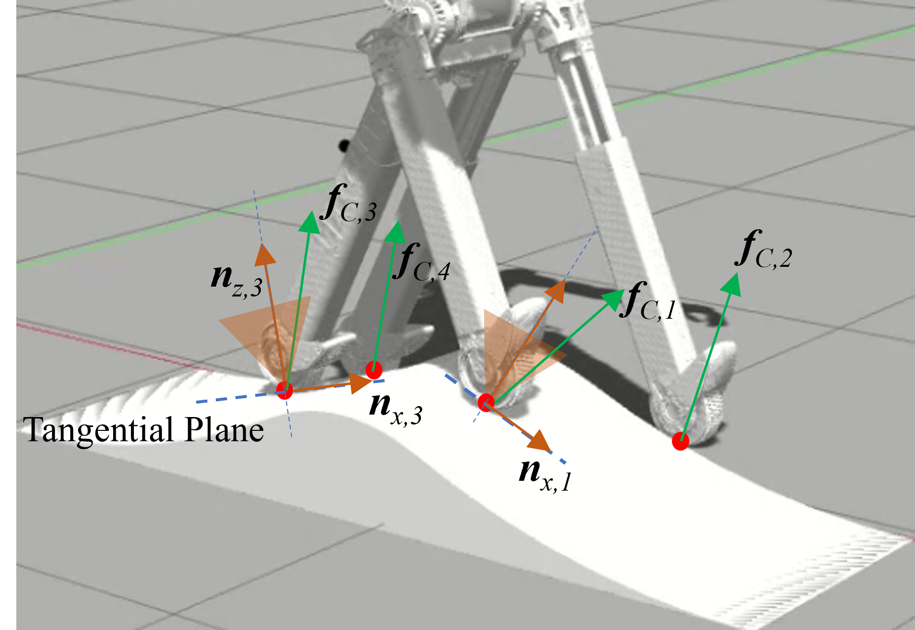
Figure 5: Terrain frame estimation. $\{\boldsymbol{n}_{x,i},\boldsymbol{n}_{y,i},\boldsymbol{n}_{z,i}\}$ is the terrain frame of $i$-th contact point. $\boldsymbol{f}_{C,i}$ is the ground contact force of $i$-th contact point.

This part we propose a novel strategy for the estimation of terrain frame $\{\boldsymbol{n}_{x},\boldsymbol{n}_{y}$,$\boldsymbol{n}_{z}\}$ shown in Fig. 5. $\boldsymbol{n}_{x}$ can be estimated directly from the wheel’s history trajectory in the forward direction, and $\boldsymbol{n}_{z}$ can be estimated from contact force of wheel-foot, because the force in this direction is more obviously affected by the robot’s own gravity. The constraint surface [23, 24] in the task space can be expressed as follows:

$$\boldsymbol{\psi}(\boldsymbol{x},\theta)=\boldsymbol{0}$$ (24)

where $\boldsymbol{\psi}\in\mathbb{R}^{m}$. Denote $\boldsymbol{J}_{\psi,x}(\boldsymbol{x},\theta)$ the constraint Jacobian matrix in the task space, $\boldsymbol{J}_{\psi,x}(\boldsymbol{x},\theta)\boldsymbol{\dot{x}}=\boldsymbol{0}$, and it also belongs to orthogonal matrix.

$$\boldsymbol{J}_{\psi,x}(\boldsymbol{x},\theta)=\lVert\frac{\partial\boldsymbol{\psi}(\boldsymbol{x},\theta)}{\partial{\boldsymbol{x}}}\lVert^{-1}\frac{\partial\boldsymbol{\psi}(\boldsymbol{x},\theta)}{\partial{\boldsymbol{x}}}$$ (25)

Denote $\boldsymbol{P}(\boldsymbol{x},\theta)$ the orthogonal projection matrix. Let $\boldsymbol{\dot{x}}_{\text{forward}}$ be the forward speed, and it is also an element of $\boldsymbol{\dot{x}}_{R}$. So we have:

$$\boldsymbol{P}(\boldsymbol{x},\theta)=\boldsymbol{I}-\boldsymbol{J}^{+}_{\psi,x}(\boldsymbol{x},\theta)\boldsymbol{J}_{\psi,x}(\boldsymbol{x},\theta)$$ (26)

$$\boldsymbol{\hat{n}}_{x}=\boldsymbol{P}\boldsymbol{\dot{x}}_{\text{forward}}{\lVert\boldsymbol{\dot{x}}_{\text{forward}}\lVert^{-1}}$$ (27)

Furthermore, the actual joint toque ${\boldsymbol{\hat{\tau}}}_{\text{ext}}$ corresponds to the contact force ${\boldsymbol{\hat{f}}}_{\text{ext}}$ can be estimated by the general momentum observer with the measurement of $\{\boldsymbol{q},{\boldsymbol{\dot{q}}},\boldsymbol{\tau}\}$.

$${\boldsymbol{\hat{\tau}}}_{\text{ext}}=F_{GM}(\boldsymbol{q},{\boldsymbol{\dot{q}}},\boldsymbol{\tau})=\boldsymbol{J}^{T}_{e}{\boldsymbol{\hat{f}}}_{\text{ext}}$$ (28)

where $F_{GM}$ is the general momentum observer algorithm function [19, 20]. So ${\boldsymbol{\hat{f}}}_{\text{ext}}$ can be obtained by the inverse solution of the above equation. Thus, $\boldsymbol{\hat{f}}_{C}$ can be derived. In fact, the estimated $\boldsymbol{\hat{f}}_{C}$ usually contains a frictional force component. So the estimated normal vector

$$\ \boldsymbol{\hat{n}}_{z}={\boldsymbol{\hat{f}}_{C,z}}/{\lVert\boldsymbol{\hat{f}}_{C,z}\lVert}$$ (29)

and

$$\ {\boldsymbol{\hat{f}}_{C,z}}={\boldsymbol{\hat{f}}_{C}-({\boldsymbol{\hat{f}}^{T}_{C}}{\boldsymbol{\hat{n}}_{x}}}){\boldsymbol{\hat{n}}_{x}}$$ (30)

Then, $\boldsymbol{\hat{n}}_{y}$ can be derived as

$$\ \boldsymbol{\hat{n}}_{y}=\boldsymbol{\hat{n}}_{z}\times\boldsymbol{\hat{n}}_{x}$$ (31)

V-C The Model-free Compensation in WBC

We use a model-free approach to derive $\boldsymbol{\tau}_{f}$.

$$\boldsymbol{\tau}_{f}=\boldsymbol{J}^{T}\boldsymbol{\sigma}(\boldsymbol{\dot{x}}(t),\boldsymbol{u}(t)){\boldsymbol{F}}_{f}(t)$$ (32)

where ${\boldsymbol{F}}_{f}(t)$ is the time-varying friction value. $\boldsymbol{u}(t)=\boldsymbol{\ddot{x}}_{\text{des}}$. $\boldsymbol{\sigma}$ is the signum friction, and it affects the direction of friction force in Eq.(18). its diagonal elements $\sigma_{i}$ is shown as

$$\sigma_{i}=\left\{\begin{array}[]{lcl}1~{}~{}~{}\mathrm{if}~{}\dot{x}_{i}>0~{}\mathrm{or}~{}(\dot{x}_{i}=0~{}\mathrm{and}~{}u_{i}(t)>0)\\ -1~{}\mathrm{if}~{}\dot{x}_{i}<0~{}\mathrm{or}~{}(\dot{x}_{i}=0~{}\mathrm{and}~{}u_{i}(t)<0)\\ 0~{}~{}~{}\mathrm{if}~{}\dot{x}_{i}=0~{}\mathrm{and}~{}u_{i}(t)=0\\ \end{array}\right.$$ (33)

It can be seen that the activation function is not only affected by $\boldsymbol{\dot{x}}$, but also affected by $\boldsymbol{u}$ at zero speed. This can effectively avoid the defects of frictionless compensation corresponding to the zero-speed transition point of the trajectory. Besides, the the update speed of differential value ${\boldsymbol{\dot{F}}}_{f}(t)$ is effected by $\boldsymbol{\sigma}$.

$${\boldsymbol{\dot{F}}}_{f}(t)=\boldsymbol{k}_{P}\boldsymbol{\sigma}({\boldsymbol{\dot{e}}}+{\boldsymbol{k}}_{\lambda}{\boldsymbol{e}})$$ (34)

where $\boldsymbol{k}_{P}$ and $\boldsymbol{k}_{\lambda}$ are the tuning parameters. $\boldsymbol{e}=\boldsymbol{x}_{\text{des}}(t)-\boldsymbol{x}(t)$ denotes the position error. ${\boldsymbol{{F}}}_{f}(t)$ can be obtained by numerical integration of ${\boldsymbol{\dot{F}}}_{f}(t)$.

VI Experiments

The WBC setup described in this article is implemented in C++. The software uses the Eigen3 library and the qpOASES quadratic progrmming library. The proposed controller was running on a 8-cores Intel Core i7-32G RAM computer with 500 $Hz$ control loop.

The experimental scene is set up in such a way that the robot walks on flat ground, uphill and downhill, cobblestone ground, wave slopes, etc. Considering the maximum extension and contraction of the legs is 35 $\mathrm{cm}$, the maximum height difference of the experimental site is set to 20 $\mathrm{cm}$. The friction coefficient of the robot’s tires with various terrains is between 0.06 and 0.12.

Here we set the friction coefficient in the algorithm to 0.1, and the uncertainty of the friction coefficient is guaranteed by the robustness of the WBC algorithm and the slip detection algorithm. During the experiment, the robot did not know the specific information about the slope and friction of the terrain. In order to demonstrate the stability of the robot manipulating objects under uncertain terrain information, we choose to hold a plate with both arms and place a bottle of water on the plate. The size of the plate is 38.5x28.5 $\mathrm{cm}$, and the weight of the water is 0.6 $\mathrm{kg}$. The friction coefficient between the plate and the bottle is 0.5, and the friction coefficient between the arms and the plate is 1.2. Throughout the process, we preset the maximum forward speed to 0.8 $\mathrm{m/s}$ and the maximum turning speed to 0.5 $\mathrm{rad/s}$. The actual navigation instructions are calculated in real time by the ROS navigation module based on the SLAM perception information.

We set the parameters in the ICC as: $M=80$, $D_{b}=600$, $K_{b}=100000$, $m_{L}=0.9$, $D_{L,\text{min}}=20$, $D_{L,\text{max}}=200$, $K_{L}=350$, $m_{R}=0.9$, $D_{L,\text{mix}}=20$, $D_{L,\text{max}}=200$, $K_{R}=350$. And we also set $D_{L}=100$, $D_{R}=100$ for comparison in ablation experiments.. The configuration-related task parameters of the robot task in the WBC are set as: the proportional and derivative parameters of the robot height task are 1000 and 20 respectively. The proportional and derivative parameters of the robot wheel-Centroid task are 800 and 10 respectively. The proportional and derivative parameters of the robot base rotation task are 300 and 15 respectively. These sets of parameters will directly determine the overall configuration of the robot.

During the entire experiment, the robot did not know the accurate information of the terrain. The upper body of the robot remained vertical based on the perception of the IMU, and the overall configuration of the robot remained unchanged. The experimental screenshots are shown in the Fig. LABEL:taskA and Fig. LABEL:taskB. The experimental terrain shape and terrain slope curves are shown in the Fig. 8. Terrain-1 mainly includes uphill, cobblestone and downhill. Terrain-2 mainly consists of wave slope. It can be seen that, through the algorithm given in Sec.V.B, the robot successfully estimates the terrain information and introduces it into the WBC solution. In the Fig.8, the maximum slope of the terrain is 0.22 $\mathrm{rad}$. In the experiment, the robot maintains a constant height throughout the entire process, and only increases its height when it cannot pass the terrain. In the Fig. 10, when going uphill, the robot’s front legs shorten to adapt to the constant height, and when going downhill, the front legs stretch to adapt to the height. And when passing a wave slope, the legs will have obvious changes in alternating shortening and lengthening.

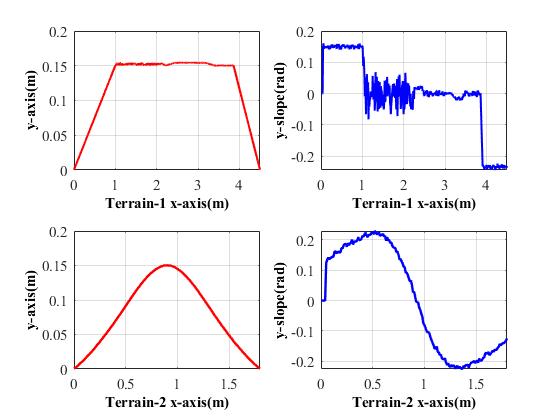
Figure 9: Curves of terrain shape (shown in up left and down left) and terrain slope (shown in up right and down right).

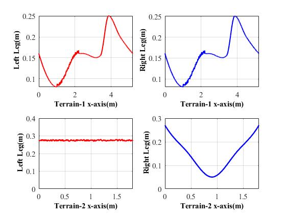
Figure 10: Extension curves of the front legs in the terrain 1 and 2.

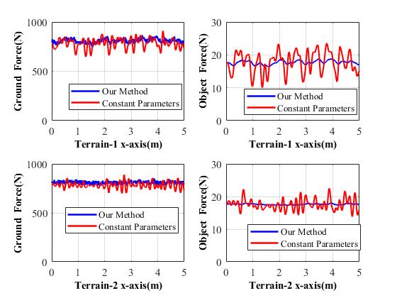
Figure 11: Curves of ground contact force(shown in up left and down left) and object contact forces(shown in up right and down right).

The experimental curves shown in Fig. 11 shows that under the action of the variable damping controller, the contact force of the robot’s upper body is relatively smooth and controlled within a reasonable range (the force fluctuation is within 18 $\mathrm{N}$). The results show that the robot can maintain the stability of the upper body transporting water while crossing different terrains. Through the algorithm in this article, the force of the robot’s upper body can be effectively controlled within a reasonable range to avoid the impact of terrain changes on the robot.

VII Conclusions

This article proposes an impedance coordinative control for our newly developed wheel-legged humanoid robot in order to cope with locomotion tasks. Such impedance coordinative control also allows the robot to maintain upper-body passive stability when carrying objects, even in challenging terrain environments. In addition, a whole-body control framework for robots that includes terrain information update and model-free compensation is proposed. The update of terrain information can timely correct the tangential and normal information of the robot’s contact point with the ground, and then update the range of the friction cone constraint. Experimental results verify that the proposed algorithms effectively support the robot in adapting to various terrains while ensuring upper-body passive stability.

References

- [1] Y. Tong, H. Liu, and Z. Zhang, “Advancements in humanoid robots: A comprehensive review and future prospects,” IEEE/CAA Journal of Automatica Sinica, vol. 11, no. 2, pp. 301–328, 2024.
- [2] S. Kuindersma, R. Deits, M. Fallon, A. Valenzuela, H. Dai, F. Permenter, T. Koolen, P. Marion, and R. Tedrake, “Optimization-based locomotion planning, estimation, and control design for the atlas humanoid robot,” Autonomous robots, vol. 40, pp. 429–455, 2016.
- [3] G. Mesesan, J. Englsberger, G. Garofalo, C. Ott, and A. Albu-Schäffer, “Dynamic walking on compliant and uneven terrain using dcm and passivity-based whole-body control,” in 2019 IEEE-RAS 19th International Conference on Humanoid Robots (Humanoids). IEEE, 2019, pp. 25–32.
- [4] N. Gupta, J. Smith, B. Shrewsbury, and B. Børnich, “2d push recovery and balancing of the eve r3-a humanoid robot with wheel-base, using model predictive control and gain scheduling,” in 2019 IEEE-RAS 19th International Conference on Humanoid Robots (Humanoids). IEEE, 2019, pp. 365–372.
- [5] N. Kashiri, L. Baccelliere, L. Muratore, A. Laurenzi, Z. Ren, E. M. Hoffman, M. Kamedula, G. F. Rigano, J. Malzahn, S. Cordasco et al., “Centauro: A hybrid locomotion and high power resilient manipulation platform,” IEEE Robotics and Automation Letters, vol. 4, no. 2, pp. 1595–1602, 2019.
- [6] B. Ma, Z. Jiang, Y. Liu, and Z. Xie, “Advances in space robots for on-orbit servicing: A comprehensive review,” Advanced Intelligent Systems, vol. 5, no. 8, p. 2200397, 2023.
- [7] M. A. Diftler, J. S. Mehling, M. E. Abdallah, N. A. Radford, L. B. Bridgwater, A. M. Sanders, R. S. Askew, D. M. Linn, J. D. Yamokoski, F. Permenter et al., “Robonaut 2-the first humanoid robot in space,” in 2011 IEEE international conference on robotics and automation. IEEE, 2011, pp. 2178–2183.
- [8] P. M. Wensing, M. Posa, Y. Hu, A. Escande, N. Mansard, and A. Del Prete, “Optimization-based control for dynamic legged robots,” IEEE Transactions on Robotics, 2023.
- [9] L. Righetti, J. Buchli, M. Mistry, and S. Schaal, “Inverse dynamics control of floating-base robots with external constraints: A unified view,” in 2011 IEEE international conference on robotics and automation. IEEE, 2011, pp. 1085–1090.
- [10] M. Hutter, H. Sommer, C. Gehring, M. Hoepflinger, M. Bloesch, and R. Siegwart, “Quadrupedal locomotion using hierarchical operational space control,” The International Journal of Robotics Research, vol. 33, no. 8, pp. 1047–1062, 2014.
- [11] C. D. Bellicoso, C. Gehring, J. Hwangbo, P. Fankhauser, and M. Hutter, “Perception-less terrain adaptation through whole body control and hierarchical optimization,” in 2016 IEEE-RAS 16th International Conference on Humanoid Robots (Humanoids). IEEE, 2016, pp. 558–564.
- [12] S. Sovukluk, J. Englsberger, and C. Ott, “Highly maneuverable humanoid running via 3d slip+ foot dynamics,” IEEE Robotics and Automation Letters, 2023.
- [13] K. Verbert, R. Tóth, and R. Babuška, “Adaptive friction compensation: a globally stable approach,” IEEE/ASME Transactions on Mechatronics, vol. 21, no. 1, pp. 351–363, 2015.
- [14] A. Dietrich and C. Ott, “Hierarchical impedance-based tracking control of kinematically redundant robots,” IEEE Transactions on Robotics, vol. 36, no. 1, pp. 204–221, 2019.
- [15] E. M. Hoffman, A. Laurenzi, L. Muratore, N. G. Tsagarakis, and D. G. Caldwell, “Multi-priority cartesian impedance control based on quadratic programming optimization,” in 2018 IEEE International Conference on Robotics and Automation (ICRA). IEEE, 2018, pp. 309–315.
- [16] J. Jo, G. Park, and Y. Oh, “Robust walking stabilization strategy of humanoid robots on uneven terrain via qp-based impedance/admittance control,” Robotics and Autonomous Systems, vol. 154, p. 104148, 2022.
- [17] M. J. Pollayil, F. Angelini, G. Xin, M. Mistry, S. Vijayakumar, A. Bicchi, and M. Garabini, “Choosing stiffness and damping for optimal impedance planning,” IEEE Transactions on Robotics, vol. 39, no. 2, pp. 1281–1300, 2022.
- [18] R. K. Rastogi and M. Tripathy, “Enhancing stability and performance of dc microgrid: A coordinated impedance reshaping controller design approach,” IEEE Transactions on Industry Applications, 2024.
- [19] M. Focchi, R. Orsolino, M. Camurri, V. Barasuol, C. Mastalli, D. G. Caldwell, and C. Semini, “Heuristic planning for rough terrain locomotion in presence of external disturbances and variable perception quality,” Advances in robotics research: From lab to market: ECHORD++: Robotic science supporting innovation, pp. 165–209, 2020.
- [20] G. Bledt, P. M. Wensing, S. Ingersoll, and S. Kim, “Contact model fusion for event-based locomotion in unstructured terrains,” in 2018 IEEE International Conference on Robotics and Automation (ICRA). IEEE, 2018, pp. 4399–4406.
- [21] L. Yang, J. Zhang, Y. Xu, K. Chen, and C. Fu, “Energy performance analysis of a suspended backpack with an optimally controlled variable damper for human load carriage,” Mechanism and Machine Theory, vol. 146, p. 103738, 2020. [Online]. Available: https://www.sciencedirect.com/science/article/pii/S0094114X19323444
- [22] C. Zhou, Y. Long, L. Shi, L. Zhao, and Y. Zheng, “Differential dynamic programming based hybrid manipulation strategy for dynamic grasping,” in 2023 IEEE International Conference on Robotics and Automation (ICRA). IEEE, 2023, pp. 8040–8046.
- [23] J. Pliego-Jiménez and M. A. Arteaga-Pérez, “Adaptive position/force control for robot manipulators in contact with a rigid surface with uncertain parameters,” European Journal of Control, vol. 22, pp. 1–12, 2015.
- [24] M. Namvar and F. Aghili, “Adaptive force-motion control of coordinated robots interacting with geometrically unknown environments,” IEEE Transactions on Robotics, vol. 21, no. 4, pp. 678–694, 2005.