Unlocking Transfer Learning for Open-World Few-Shot Recognition

Abstract

Few-Shot Open-Set Recognition (FSOSR) targets a critical real-world challenge, aiming to categorize inputs into known categories, termed closed-set classes, while identifying open-set inputs that fall outside these classes. Although transfer learning where a model is tuned to a given few-shot task has become a prominent paradigm in closed-world, we observe that it fails to expand to open-world. To unlock this challenge, we propose a two-stage method which consists of open-set aware meta-learning with open-set free transfer learning. In the open-set aware meta-learning stage, a model is trained to establish a metric space that serves as a beneficial starting point for the subsequent stage. During the open-set free transfer learning stage, the model is further adapted to a specific target task through transfer learning. Additionally, we introduce a strategy to simulate open-set examples by modifying the training dataset or generating pseudo open-set examples. The proposed method achieves state-of-the-art performance on two widely recognized benchmarks, miniImageNet and tieredImageNet, with only a 1.5% increase in training effort. Our work demonstrates the effectiveness of transfer learning in FSOSR.

1 Introduction

Few-shot learning (FSL) has got a lot of attention due to the importance in enabling models to adapt to novel tasks using a few examples (e.g., $N$-way $K$-shot: a task involving $N$ distinct classes, each represented by $K$ examples) [42, 17, 37, 34, 27, 10]. However, in practical applications, FSL models inevitably encounter instances that do not belong to the $N$ classes, also known as open-set instances. Addressing this challenge has led to the emergence of the field of few-shot open-set recognition (FSOSR) [24, 16, 19, 15, 41].

In FSOSR, if two $N$-way $K$-shot FSOSR tasks have distinct closed sets, their corresponding open sets will also differ. This interdependence presents a key challenge when adapting to novel tasks in FSOSR. Namely, it is essential to redefine not only the closed set but also the open set, since the open set is inherently shaped by its closed set. Consequently, the open set lacks a universal definition across various FSOSR tasks; instead, it requires contextual consideration based on the closed set of a specific target task.

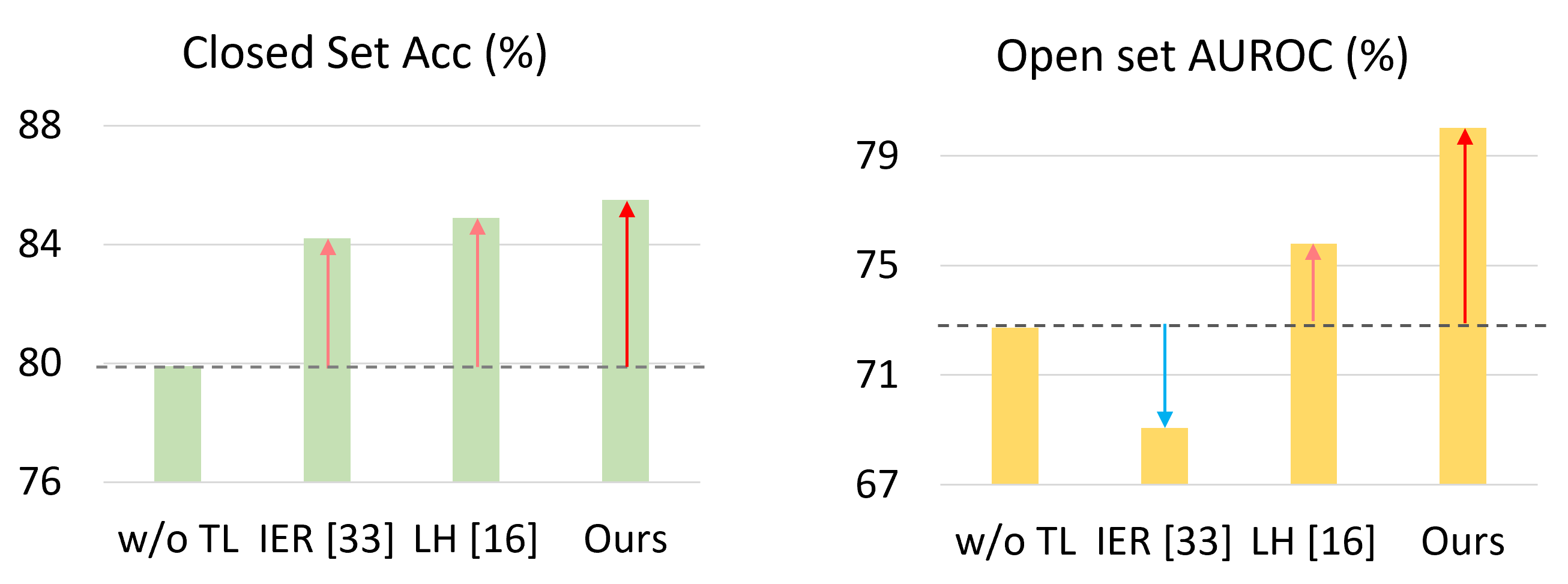
Figure 1: Difficulty of straightforward extension of the transfer learning from FSL methods [34, 17] to FSOSR. Compared to the pre-trained model without transfer learning (w/o TL), in open-set recognition, [34, 17] are less effective as much as in closed-set, or even degrade the performance.

Despite recent advancements in the field, current works [24, 16, 19, 15, 41] have commonly focused on leveraging prior knowledge from a large training dataset. Then, they frequently struggle to balance closed-set accuracy with open-set recognition capabilities, often prioritizing open-set recognition at the expense of closed-set accuracy. Then, these approaches face challenges in achieving broad generalization across various benchmarks. In this work, we bring attention to the novel application of transfer learning within this field. Transfer learning [14, 7, 6, 30] has been extensively studied and demonstrated its efficacy leveraging a pre-trained model to generalize it to other tasks. Recent FSL methods [31, 34, 39, 17, 35] have shown the efficacy of this approach. However, when they come to FSOSR, open-set examples are inherently not present, which significantly undermines the effect of transfer learning in terms of open-set recognition. Then, as in Fig. 1, the naive extension of the transfer learning techniques of FSL, e.g. IER-distill [34] and Label Halluc. [17] fails to attain the same level of improvement in open-set recognition as seen in closed set, or even results in decreased result.

Tackling this point, we propose a two-staged FSOSR learning framework. Our method involves two stages: open-set aware meta-learning (OAL) and open-set free transfer learning (OFL). During the meta-learning stage, our objective extends beyond the meta-training of the feature encoder; we also aim to establish a universal open-set representation. This equips us with a decent starting point for the subsequent open-set free transfer learning. In the transfer learning stage, we commence by initializing the model using the parameters obtained from the meta-learning stage. To counteract the absence of open-set examples, we develop two alternative open-set sampling strategies. The first approach curates a training dataset of the previous stage as a source of open-set examples for open-set free transfer learning. For more pragmatic application, our second strategy is confined to the closed-set examples present in the target task, and exploits an episodic learning framework. Here, we generate pseudo FSOSR episodes by randomly dividing the closed-set categories into a closed set and a pseudo open set. As a result, our OAL-OFL method attains a marked enhancement in performance metrics on the standard FSOSR benchmarks as depicted in Fig. 1 while incurring a minimal extra training expense of only 1.5% compared to training without transfer learning. This allows OAL-OFL to surpass the existing state-of-the-art (SOTA) methods.

Our contributions are summarized as four-fold:

• We introduce a novel two-staged learning called OAL-OFL, bringing transfer learning to FSOSR for the first time with only a minimal additional cost.

• We show the importance of preparing the model through open-set aware meta-learning, which is a sturdy starting point for transfer learning.

• We suggest two breakthroughs to handle the lack of open-set examples during the transfer learning stage.

• By leveraging the effectiveness of transfer learning, our proposed OAL-OFL achieves SOTA on miniImageNet and tieredImageNet datasets. This underscores its ability to generalize across various tasks, enhancing both closed-set classification accuracy and open-set recognition capabilities.

2 Related Works

FSL [9] can be streamlined into two approaches: meta-learning and transfer learning. Meta-learning, also known as learning-to-learn, can be categorized into optimization and metric-based methods. Optimization-based methods [10, 11, 22, 27] involve training a meta-learner to adapt quickly to new tasks through a few optimization steps by learning adaptation procedures. In contrast, metric-based methods [20, 37, 40, 42] use a common feature embedding space where target classes of a new task can be distinguished using a distance metric. Recently, transfer learning-based approaches [31, 34, 17, 35] have been suggested with superior results where a model trained on a large-scale base dataset is fine-tuned to a few-shot task with a small number of support examples. Our approach aligns with the transfer learning-based approaches of the few-shot classification, but transfer learning has yet to be explored in the context of FSOSR.

OSR aims to identify in-distribution samples within a closed set, and simultaneously detect the out-of-distribution samples from unseen classes. Early approaches focused on the confidence level and proposed various approaches such as using extreme value theory [1, 2, 13, 36]. Recently, there has been a growing interest in generative model-based approaches [28, 29, 38], which leverage the different reconstruction behavior between in-distribution and out-of-distribution samples. On the other hand, our method aligns more closely with distance-based approaches [18, 25, 43], particularly those that specify open-set representation [3, 45]. However, OSR methods inherently assume the distinct and fixed class pools for the closed and open sets, which is not feasible in FSOSR, where both sets vary depending on a task. As a result, it is hard to straightforwardly apply the conventional OSR techniques to FSOSR.

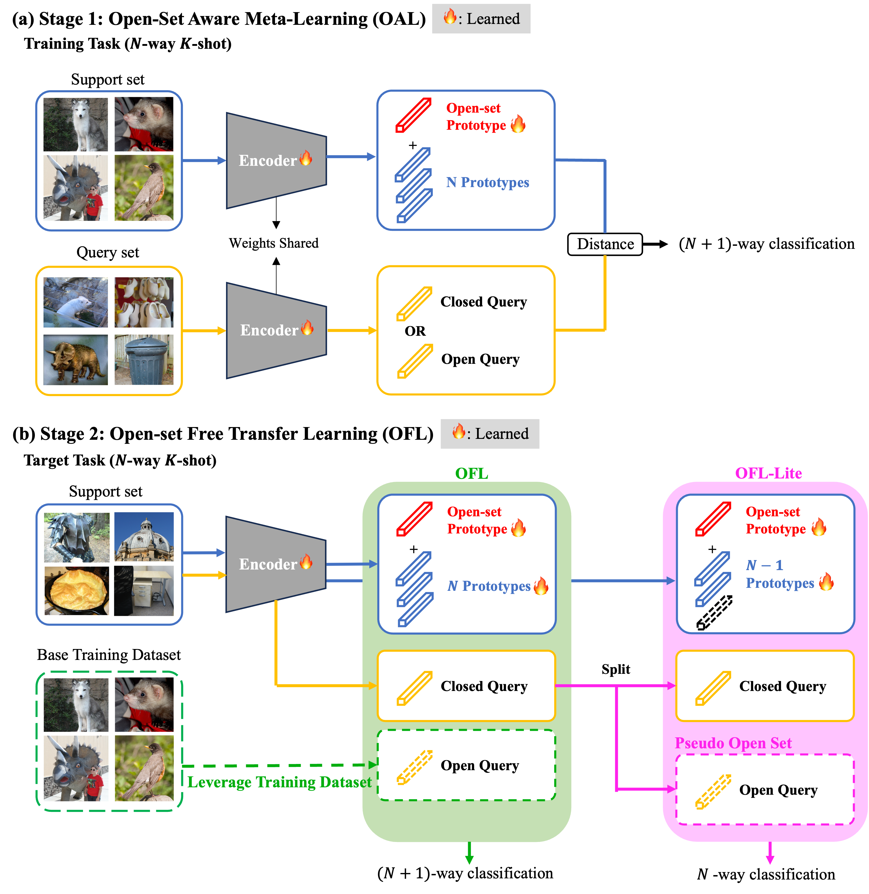
Figure 2: Overall training framework of OAL-OFL. (a) In Stage 1, the feature encoder and a learnable open-set prototype undergo distance-based meta-learning [37] with an additional class representing the open set. (b) In Stage 2, feature encoder and prototypes are further transfer-learned to the target task under an open-set-free condition. Open-set training examples can be alternatively drawn from the base training dataset (green) or from a subset of the closed-set categories that is randomly selected as a pseudo open set (purple).

FSOSR. Compared to few-shot classification and OSR, FSOSR has been less explored. PEELER [24] introduced FSOSR task and aimed to maximize the entropy of open-set examples with Gaussian embeddings. They employed OSR approach [1] of detecting open-set examples based on the largest class probability. SnaTCHer [16] used transformation consistency that similar examples remain closer after a set-to-set transformation. TANE [15] and D-ProtoNet [19] proposed a task-dependent open-set generator using support examples. Considering low-level features as well as semantic-level ones, GEL [41] designed a local-global energy score to measure the deviation of the input from the closed-set examples. The aforementioned methods primarily employ the representative metric learning approach, ProtoNets [37], and face difficulties in achieving generalization across diverse benchmarks. Our proposed approach, however, involves a two-stage learning process. The first stage focuses on meta-learning to train a task-independent open-set classifier that serves as an effective initialization for the second stage of transfer learning.

3 Proposed Method

We present the proposed two-stage transfer learning process, dubbed OAL-OFL. The overall framework of OAL-OFL is depicted in Fig. 2. First, we describe the first stage, open-set aware meta-learning, where a universal FSOSR metric space is obtained by learning the feature encoder and a learnable open-set prototype. Then, we elaborate on the open-set free transfer learning stage, especially suggesting two approaches to resolve the challenges of the absence of open-set examples.

Problem definition. The goal of FSOSR is two-fold: to classify an input query into one of the closed-set categories or to reject it as belonging to the associated open-set categories. Formally, an $N$-way $K$-shot FSOSR task can be represented as $\mathcal{T}=\{S,Q,\tilde{Q}\ |\mathcal{C},\tilde{\mathcal{C}}\}$, where $C$ denotes a set of $N$ closed-set categories. The closed set is described by a support set $S$ which includes $K$ examples for each category, i.e. $\{x_{i},y_{i}\}_{1}^{|S|}$ and $|S|=NK$. Here, $x$ represents the input data, while $y$ indicates its corresponding label. The query set for $C$ is denoted by $Q$. Distinctively, FSOSR also accommodates open-set queries $\tilde{Q}$, which belong to categories, $\tilde{\mathcal{C}}$, that do not intersect with $C$ and are not explicitly defined.

3.1 Stage-1: Open-set Aware Meta-Learning

We commence by meta-learning a metric space, which serves as a general starting point to tune the model to a specific target task in the open-set free transfer learning of Stage-2. As depicted in Fig. 2 (a), this meta-learning stage involves the simultaneous training of the feature encoder $f_{\theta}$ and a learnable open-set prototype $c_{\phi}$. These are learned using FSOSR tasks drawn from the base training dataset, denoted as $\mathcal{D}_{\mathrm{bs}}$. Though the definition of open set varies depending on $\mathcal{C}$, the $c_{\phi}$ is desired to be task-independent across $\forall\mathcal{C}$. Given the complexities involved in learning the task-specific open set classifier during Stage-2, the effective training of a reliable $c_{\phi}$ serves as a crucial link to bridge the two stages.

In specific, given an $N$-way $K$-shot FSOSR task, $\mathcal{T}\sim\mathcal{D}_{\mathrm{bs}}$, we conceptualize this as the $(N+1)$-way classification problem. In this framework, the $(N+1)$th class is designated as the open-set class. For $n$-th class of $\mathcal{C}$, the classifier is formulated as the prototype $c_{n}$ which is defined as the mean feature vector over its $K$ examples, i.e., $c_{n}=\frac{1}{K}\sum_{m=1}^{K}{f_{\theta}(x_{m})}$ [37]. Here, $f_{\theta}(x)$ produces a $D$-dimensional feature vector. Concurrently, for the open-set class, the corresponding classifier is characterized by the learnable open-set prototype $c_{\phi}$.

Subsequently, the classification probability is

$$p(y=n|x)= \frac{e^{-a\cdot d(c_{\phi},f_{\theta}(x))+b}}{e^{-a\cdot d(c_{\phi},f_{\theta}(x))+b}+\sum_{n^{\prime}=1}^{N}{e^{-d(c_{n^{\prime}},f_{\theta}(x))}}},$$

$$\text{if }n=N+1,$$

$$p(y=n|x)= \frac{e^{-d(c_{n},f_{\theta}(x))}}{e^{-a\cdot d(c_{\phi},f_{\theta}(x))+b}+\sum_{n^{\prime}=1}^{N}{e^{-d(c_{n^{\prime}},f_{\theta}(x))}}},$$

$$\text{Otherwise},$$ (1)

where $d$ is a distance metric. Specifically, we use the squared Euclidean distance, $d(v,v^{\prime})=||v-v^{\prime}||^{2}$. In addition, scalars $a$ and $b$ are also learned to calibrate the distance to $c_{\phi}$, inspired by D-ProtoNets [19]. This calibration enables that $c_{\phi}$ is solely accountable for representing open sets of various tasks. For the loss function, we utilize the cross-entropy (CE) loss which is formulated as:

$$\mathcal{L}_{\textrm{CE}}(x_{i},y_{i})= -{\log{p_{\theta}(y=y_{i}|x_{i})}}.$$ (2)

We further utilize the masked CE loss [45], defined as:

$$\mathcal{L}_{\textrm{Mask}}(x_{i},y_{i})=-{\log{p_{\theta\char 92\relax y_{i}}(y=N+1|x_{i})}},$$ (3)

where $p_{\theta\char 92\relax y_{i}}$ denotes the $N$-way classification probability, excluding the ground-truth label $y_{i}$. This loss term effectively creates pseudo open-set tasks by disregarding the true label. More precisely,

$$p_{\theta\char 92\relax y_{i}}(y=N+1|x_{i})=\frac{e^{-d_{N+1}}}{e^{-d_{N+1}}+\sum_{n^{\prime}=1,n^{\prime}\neq y_{i}}^{N}{e^{-d(c_{n^{\prime}},f_{\theta}(x_{i}))}}},$$

where we let $d_{N+1}=a\cdot d(c_{\phi},f_{\theta}(x_{i}))+b$ for brevity.

Overall, we learn $f_{\theta}$, $c_{\phi}$, $a$, and $b$ as

$$\theta^{*}_{1}, \phi^{*}_{1},a^{*}_{1},b^{*}_{1}=\operatorname*{arg\,min}_{\theta,\phi,a,b}\{\mathbb{E}_{x\in\tilde{Q}}\mathcal{L}_{\textrm{CE}}(x,N+1)$$

$$+\mathbb{E}_{(x,y)\in Q}\{\mathcal{L}_{\textrm{CE}}(x,y)+\mathcal{L}_{\textrm{Mask}}(x,y)\}\}.$$ (4)

3.2 Stage-2: Open-set Free Transfer Learning

In this stage, we consider a target task, denoted as $\mathcal{T}_{\mathrm{te}}=\{S_{\mathrm{te}},Q_{\mathrm{te}},\tilde{Q}_{\mathrm{te}}\ |\mathcal{C}_{\mathrm{te}},\tilde{\mathcal{C}}_{\mathrm{te}}\}$, which is also configured as an $N$-way $K$-shot task. Note that $Q_{\mathrm{te}}$ and $\tilde{Q}_{\mathrm{te}}$ are utilized solely for the purposes of inference during test. The initial values of the learnable parameters are inherited from results of Stage-1. Specifically, $f_{\theta}$, $a$ and $b$ are imprinted as $f_{\theta^{*}_{1}}$, $a^{*}_{1}$ and $b^{*}_{1}$, respectively. We aim to train them alongside $(N+1)$-way classifiers. These classifiers are represented as $\{w_{1},\cdots,w_{N+1}\}$, where each $w_{n}\in\mathbb{R}^{D}$. The first $N$ classifiers are set as the prototypes of the corresponding classes in $C_{\mathrm{te}}$. The open-set classifier $w_{N+1}$ is initialized using $c_{\phi_{1}^{*}}$.

To ensure consistency with the meta-learned metric space, we compute the classification probability of each query based on the Euclidean distance as in Eq. (3.1). Then, during the transfer learning, we optimize $f_{\theta}$ and the classifier $g_{\psi}=\{w_{1},\cdots,w_{N+1},a,b\}$.

Since $\mathcal{T}_{\mathrm{te}}$ lacks cues to learn the open-set classifier $w_{N+1}$, we suggest two approaches: i) sampling from the base training dataset $\mathcal{D}_{\mathrm{bs}}$ of Stage-1, and ii) sampling from the closed set $C_{\mathrm{te}}$ of $\mathcal{T}_{\mathrm{te}}$ itself.

3.2.1 Open-set sampling from base training dataset

Notice that in the context of FSL, the closed-set categories $C_{\mathrm{te}}$ in $\mathcal{T}_{\mathrm{te}}$ are exclusive with $\mathcal{D}_{\mathrm{bs}}$. As a result, we can exploit $D_{\mathrm{bs}}$ as a pool of open-set examples for $\mathcal{T}_{\mathrm{te}}$. Specifically, as in the green-colored of Fig. 2(b), we randomly select $M$ examples from $\mathcal{D}_{\mathrm{bs}}$ at every iteration of the transfer learning to serve as open-set examples.

Then, the model is optimized as:

$$\theta^{*}_{2},\psi^{*}_{2}= \operatorname*{arg\,min}_{\theta,\psi}\{\mathbb{E}_{(x,y)\in S_{\mathrm{te}}}\mathcal{L}_{\text{CE}}(x,y)$$

$$+\mathbb{E}_{x\sim D_{\mathrm{bs}}}\mathcal{L}_{\text{CE}}(x,N+1)\}.$$ (5)

We call this unified process of Stage-1 and 2 with the base training dataset as OAL-OFL. In the following section, we will introduce the OAL-OFL with a more practical open-set sampling, dubbed OAL-OFL-Lite.

3.2.2 Pseudo open-set sampling from closed set

In real-world scenarios, $\mathcal{T}_{\mathrm{te}}$ encompasses various categories, and we cannot guarantee that the closed set $C_{\mathrm{te}}$ is not overlapped with the categories of $\mathcal{D}_{\mathrm{bs}}$. Additionally, after the meta-learning stage, the large-scale $\mathcal{D}_{\mathrm{bs}}$ may not be affordable due to practical constraints. To address these issues, we introduce OAL-OFL-Lite which operates with no necessity of $\mathcal{D}_{\mathrm{bs}}$.

Our strategy is the episodic random class sampling from the closed set $C_{\mathrm{te}}$ itself to learn the open set. As exemplified in the purple-colored of Fig. 2(b), we iteratively partition $C_{\mathrm{te}}$ into the mutually exclusive subsets $\acute{C}_{\mathrm{te}}$ and $\tilde{C}_{\mathrm{te}}$. Subsequently, their corresponding support sets $\acute{S}_{\mathrm{te}}$ and $\tilde{S}_{\mathrm{te}}$ extracted from $S_{\mathrm{te}}$ are used to transfer-learn the closed and open sets, respectively. Hence, we call $\tilde{C}_{\mathrm{te}}$ pseudo open set. Through this iterative pseudo open-set sampling, we can effectively learn the open-set classifier as well as the closed-set ones.

Then, the model is optimized by the CE losses as

$$\theta^{*}_{2},\psi^{*}_{2}= \operatorname*{arg\,min}_{\theta,\psi}\{\mathbb{E}_{(x,y)\in\acute{S}_{\mathrm{te}}}\mathcal{L}_{\text{CE}}(x,y)$$

$$+\mathbb{E}_{x\in\tilde{S}_{\mathrm{te}}}\mathcal{L}_{\text{CE}}(x,|\acute{C}_{\mathrm{te}}|+1)\}.$$ (6)

where the open set is mapped to $(|\acute{C}_{\mathrm{te}}|+1)$th class and detected by $w_{N+1}$ in every iteration. Moreover, we empirically found that the open-set representation tends to be overfitted to a testing task in OAL-OFL-Lite. Hence, we freeze $w_{N+1}$ once it is initialized by the $c_{\phi_{1}^{*}}$. For more comprehensive understanding, we include Algorithm 1.

Algorithm 1 OAL-OFL

Stage-1. Meta-Learn FSOSR Metric Space

Require: Dataset $\mathcal{D}_{\mathrm{bs}}$, encoder $f_{\theta}$.

1:Initialize $c_{\phi}$, $a$, and $b$.

2:for # of training episodes do

3:     Sample a task $\mathcal{T}=\{S,Q,\tilde{Q}|\mathcal{C},\tilde{\mathcal{C}}\}$ $\triangleright$ A training episode

4:     $c_{n}=\frac{1}{K}\sum_{m=1}^{K}{f_{\theta}(x_{m})}$, for $n\in\mathcal{C}\text{\;and\;}y_{m}=n$ $\triangleright$ Prototype

5:     $c_{1},\cdots,c_{N}=\text{LayerTaskNorm}(c_{1},\cdots,c_{N})$ $\triangleright$ Apply LayerTaskNorm [16]

6:     Update $\theta,\phi,a,b=$$\operatorname*{arg\,min}_{\theta,\phi,a,b}\{\mathbb{E}_{x\in\tilde{Q}}\mathcal{L}_{\textrm{CE}}(x,N+1)+\mathbb{E}_{(x,y)\in Q}\{\mathcal{L}_{\textrm{CE}}(x,y)+\mathcal{L}_{\textrm{Mask}}(x,y)\}\}$

7:end for

Ensure: $\theta^{*}_{1},\phi^{*}_{1},a^{*}_{1},b^{*}_{1}=\theta,\phi,a,b$

Stage-2. Transfer Learning

Require: Dataset $\mathcal{D}_{\mathrm{bs}}$ and $\mathcal{D}_{\mathrm{te}}$, $\theta^{*}_{1},\phi^{*}_{1},a^{*}_{1},b^{*}_{1}$

1:Initialize: $f_{\theta}$ with $\theta^{*}_{1}$

2:$c_{n}=\frac{1}{K}\sum_{m=1}^{K}{f_{\theta}(x_{k})}$, for $n\in\mathcal{C}_{\mathrm{te}}\text{\;and\;}y_{m}=n$

3:Initialize: $g_{\psi}$ with $\phi^{*}_{1},a^{*}_{1},b^{*}_{1},c_{1},\cdots,c_{N}$.

4:for # of iterations do

5:     Update $\theta,\psi=\operatorname*{arg\,min}_{\theta,\psi}\{\mathbb{E}_{(x,y)\in S_{\mathrm{te}}}\mathcal{L}_{\text{CE}}(x,y)+\mathbb{E}_{x\sim D_{\mathrm{bs}}}\mathcal{L}_{\text{CE}}(x,N+1)\}$

6:end for

Ensure: $\theta^{*}_{2},\psi^{*}_{2}=\theta,\psi$

4 Experimental Results

4.1 Implementation Details

In line with established FSOSR approaches [24, 16, 15, 41], we conducted experiments using ResNet12 [21] as the feature encoder on miniImageNet [40] and tieredImageNet [33] benchmarks, with pre-training of the feature encoder accomplished on the corresponding base training dataset for each benchmark through the well-known FSL method, FEAT [42]. MiniImageNet is comprised of 100 categories each with 600 examples. These categories are divided into 64, 16, and 20 classes for training, validation, and testing purposes, respectively [32]. TierdImageNet consists of 608 categories and a total of 779,165 samples, which are divided into 351, 97, and 160 classes for training, validation, and testing, respectively.

Training details. Stage-1 employs episodic learning on the base training dataset, $\mathcal{D}_{\mathrm{bs}}$, and trains the model for 20,000 episodes using the SGD optimizer with the Nesterov momentum [26] and the weight decay of 5e-4. The learning rates are initialized to 2e-4 and 2e-5 for the encoder and the learnable open-set prototype, respectively, and then decayed by multiplying 0.5 every 40 iterations. Each episode consists of a combination of closed-set categories and an equal number of open-set categories, each containing 15 queries. The distance adjusting factors $a$ and $b$ are initialized to 1 and 0, respectively. Layer-task normalization [16] is used as the embedding adaptation, which is discarded after the initialization of the classifiers in Stage-2.

In Stage-2, the proposed transfer learning is performed for 300 iterations on each testing task using the SGD optimizer. For OAL-OFL, the learning rates for the feature encoder and classifier are set to 2e-4 and 2e-3, respectively. For OAL-OFL-Lite, the learning rate is 2e-4 for both. The weight decay and momentum are set to 5e-4 and 0.9. For episode configuration in OAL-OFL-Lite, one closed-set class is randomly sampled as the pseudo open set at every iteration.

Evaluation protocol. We use the predicted probability for $(N+1)$th class as an open-set score and report threshold-free measurement AUROC [5, 8]. For closed-set evaluation, we predict the class with the highest probability among closed-set categories and report top-1 accuracy (Acc).

Compared methods. We conduct a comparative analysis of our OAL-OFL method against various existing approaches, encompassing both FSL methods such as [37, 42] and FSOSR methods [24, 16, 15, 41].

Table 1: Comparative results on the miniImageNet and tieredImageNet. Averages of Acc (%) and AUROC (%) over 600 tasks are reported with 95% confidence interval (*: reproduced numbers, ^†: results from [16]). For each case, bold and underlined scores indicate the best and second-best results.

Methods	1-shot			5-shot
	Acc.	AUROC		Acc.	AUROC
miniImageNet
ProtoNets[37]†	64.01 $\pm$ 0.9	51.81 $\pm$ 0.9		80.09 $\pm$ 0.6	60.39 $\pm$ 0.9
FEAT [42]†	67.02 $\pm$ 0.9	57.01 $\pm$ 0.8		82.02 $\pm$ 0.5	63.18 $\pm$ 0.8
PEELER [24]†	65.86 $\pm$ 0.9	60.57 $\pm$ 0.8		80.61 $\pm$ 0.6	67.35 $\pm$ 0.8
SnaTCHer-F [16]	67.02 $\pm$ 0.9	68.27 $\pm$ 1.0		82.02 $\pm$ 0.5	77.42 $\pm$ 0.7
SnaTCHer-T [16]	66.60 $\pm$ 0.8	70.17 $\pm$ 0.9		81.77 $\pm$ 0.5	76.66 $\pm$ 0.8
SnaTCHer-L [16]	67.60 $\pm$ 0.8	69.40 $\pm$ 0.9		82.36 $\pm$ 0.6	76.15 $\pm$ 0.8
ATT [15]	67.64 $\pm$ 0.8	71.35 $\pm$ 0.7		82.31 $\pm$ 0.5	79.85 $\pm$ 0.6
ATT-G [15]	68.11 $\pm$ 0.8	72.41 $\pm$ 0.7		83.12 $\pm$ 0.5	79.85 $\pm$ 0.6
GEL [41]	68.26 $\pm$ 0.9	73.70 $\pm$ 0.8		83.05 $\pm$ 0.6	82.29 $\pm$ 0.6
OAL-OFL	69.78 $\pm$ 0.8	73.88 $\pm$ 0.7		85.49 $\pm$ 0.7	83.13 $\pm$ 0.6
OAL-OFL-Lite	69.15 $\pm$ 0.8	72.21 $\pm$ 0.9		85.61 $\pm$ 0.6	81.11 $\pm$ 0.6
tieredImageNet
ProtoNets[37]†	68.26 $\pm$ 1.0	60.73 $\pm$ 0.8		83.40 $\pm$ 0.7	64.96 $\pm$ 0.8
FEAT [42]†	70.52 $\pm$ 1.0	63.54 $\pm$ 0.7		84.74 $\pm$ 0.7	70.74 $\pm$ 0.8
PEELER [24]†	69.51 $\pm$ 0.9	65.20 $\pm$ 0.8		84.10 $\pm$ 0.7	73.27 $\pm$ 0.7
SnaTCHer-F [16]	70.52 $\pm$ 1.0	74.28 $\pm$ 0.8		84.74 $\pm$ 0.7	82.02 $\pm$ 0.6
SnaTCHer-T [16]	70.45 $\pm$ 1.0	74.84 $\pm$ 0.8		84.42 $\pm$ 0.7	82.03 $\pm$ 0.7
SnaTCHer-L [16]	70.85 $\pm$ 1.0	74.95 $\pm$ 0.8		85.23 $\pm$ 0.6	80.81 $\pm$ 0.7
ATT [15]	69.34 $\pm$ 1.0	72.74 $\pm$ 0.8		83.82 $\pm$ 0.6	78.66 $\pm$ 0.7
ATT-G [15]	70.58 $\pm$ 0.9	73.43 $\pm$ 0.8		85.38 $\pm$ 0.6	81.64 $\pm$ 0.6
GEL [41]	70.50 $\pm$ 0.9	75.86 $\pm$ 0.8		84.60 $\pm$ 0.7	81.95 $\pm$ 0.7
OAL-OFL	71.73 $\pm$ 0.5	75.88 $\pm$ 0.6		86.75 $\pm$ 0.6	83.36 $\pm$ 0.6
OAL-OFL-Lite	70.80 $\pm$ 0.9	73.67 $\pm$ 0.7		86.66 $\pm$ 0.6	82.22 $\pm$ 0.6

4.2 Comparative Assessment

Table 1 presents a comparison between our OAL-OFL and baselines in 5-way {1, 5}-shot settings on miniImageNet and tieredImageNet. The objective of FSOSR is to excel in open-set recognition while simultaneously maintaining high closed-set accuracy. Whereas prior methods have predominantly concentrated on open-set recognition, our approach has demonstrated significant improvements in closed-set accuracy, showcasing clear advantages over these earlier techniques.

Since FSL approaches [37, 42] were not designed for FSOSR, we applied them to FSOSR in a straightforward manner as in [16]. In brief, in the FSL methods, the open-set detection score is computed by taking the negative of the largest classification probability [23].

Compared to the FSOSR methods, PEELER, SnaTCHers and ATT, both OAL-OFL and OAL-OFL-Lite show notably better generalized capabilities, as reflected by their Acc and AUROC across datasets. It is observed that the previous approaches exhibit a particular bias towards miniImageNet. ATT-G improves ATT by using the base class prototypes to enhance closed-set prototypes. Nevertheless, it is even worse than our OAL-OFL-Lite which does not use the base training dataset. GEL makes predictions for both pixel-wise and semantic-wise by adding a 2D convolutional block on top of the SnaTCHer-F. It attained the previous SOTA in miniImageNet, but not in all measures. Whereas we achieve SOTA performance in all cases. In 1-shot setting, we slightly outperform GEL in AUROC, but are much better in Acc (1.52% in miniImageNet and 1.23% in tieredImageNet). Notice that in FSOSR, both closed-set classification and open-set detection are important. In 5-shot setting, our method shows clear SOTA performance in both Acc and AUROC. In specific, 2.59% Acc and 0.84% AUROC in miniImageNet, and 2.15% Acc and 1.41% in tieredImageNet. Namely, when only a few examples per class are increased (one to five), the proposed open-set free transfer learning more faithfully makes it beneficial. Also, even without the base training dataset, OAL-OFL-Lite surpasses or is comparable to the existing FSOSR methods in both datasets. Therefore, we conclude that our two-stage approach successfully pioneers transfer learning for FSOSR.

Table 2: Ablation analysis on stages in the proposed OAL-OFL.

Stage-1	Stage-2	1-shot			5-shot
		Acc.	AUROC		Acc.	AUROC
Naive TL to closed set		66.05	62.38		84.21	69.07
Stage-2 only + regul.		56.97	67.78		78.98	76.72
	$\checkmark$	56.72	67.47		78.59	76.64
$\checkmark$		67.95	71.81		82.76	80.91
$\checkmark$	$\checkmark$	69.78	73.88		85.49	83.13

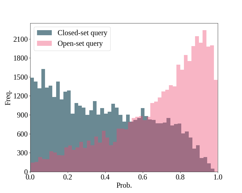
(a)

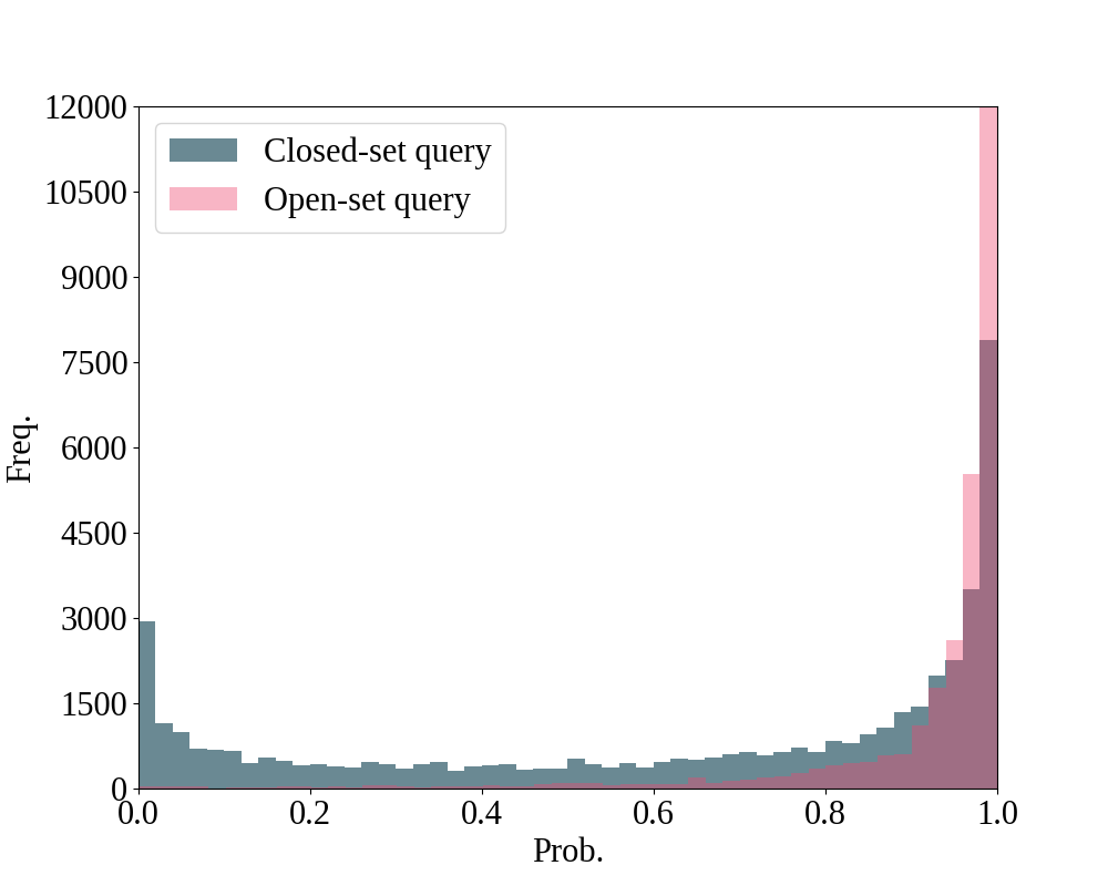
(b)

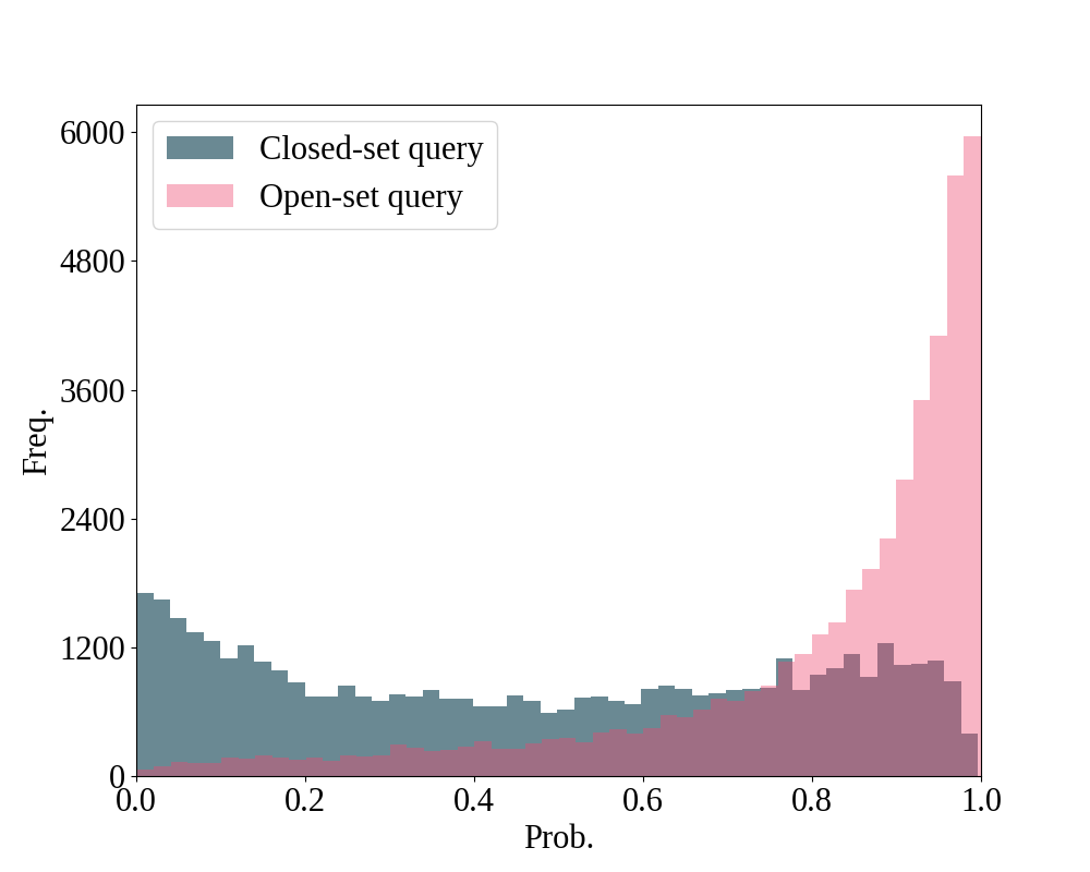
(c)

Figure 3: Distribution of the classification probabilities of closed-set and open-set queries to the open-set class. Closed-set and open-set queries are represented in green and red, respectively.

4.3 Analysis

In this section, we extensively analyze the proposed method on miniImageNet. More analyses are in the supplementary materials.

Difficulty of TL in FSOSR. To see the efficacy of the respective stage of our method especially in FSOSR, we first analyze the proposed OAL-OFL comparing with two straightforward transfer learning schemes in Table 10. First, in ‘Naive TL to closed set’ of the first row, we conduct a naive transfer learning [34] without the base training dataset. Namely, the model is fit to $N$-way closed-set classification through linear regression [4], and rejects the open-set queries thresholding max-probability [1]. This naive approach shows severely low performance, which indicates the difficulty of FSOSR transfer learning. Second, in ‘Stage-2 only + regul.,’ the pseudo-label-based regularization exploits the base training dataset to compute the Kullback–Leibler divergence between the pre-trained model and transfer-learned model, which showed promising results in transfer learning for FSL [17]. Skipping Stage-1, we can apply this regularization technique during transfer learning which is ‘Stage-2 only + regul.’ This approach (single-stage + regularization) shows only slight improvement compared to the case of only Stage-2 (1st row of the lower part of Table 10). Whereas, our OAL-OFL achieves meaningful transfer learning results by combining the two stages.

Two-stage training (OAL-OFL). To demonstrate the impact of the proposed two-stage training approach, we first ablate the stages in Table 10 for OAL-OFL. When Stage-1 is skipped, the open-set classifier $w_{N+1}$, and scalars ($a,b$) are initialized in random and (1,0), respectively in Stage-2. Relying solely on Stage-2 causes overfitting to the training examples. Then, it leads to highly degenerated results of 56.72% and 78.59% for 1- and 5-shot closed-set classification Acc, respectively, and 67.47% and 76.64% for 1- and 5-shot open-set detection AUROC, respectively. These results highlight that the open-set aware meta-learning of Stage-1 is critical for the success of transfer learning in FSOSR.

Notice that, in ATT-G [15], the base training dataset calibrates the closed-set classifiers even in testing phase, but it marginally improves ATT [15] (see Table 1). Whereas, in the proposed OAL-OFL, the use of the base training dataset during the open-set free training of Stage-2 gives notable improvement. Applied on top of Stage-1, Stage-2 attains notably improved results by 1.83% and 2.70% in Acc, and 2.07% and 2.22% in AUROC for 1- and 5-shot respectively.

In Fig. 6, we present a visualization of the distributions of classification probability towards the open-set class, derived from both closed-set and open-set queries. The visualization reveals that, in the scenario labeled as ‘Stage-2 only,’ where the open-set aware meta-learning is absent, a majority of the queries are assigned high probabilities of belonging to the open-set, irrespective of their actual membership to the closed or open set. Converserly, in ‘Stage-1 only’ scenario, a significant number of closed-set queries are still attributed probabilities exceeding 0.5. On the other hand, in OAL-OFL, it is observed that the majority of open-set queries attain significantly high probabilities of being classified as the open-set, while the probabilities for closed-set queries are effectively suppressed. This distinct separation in the classification probabilities for open and closed-set queries allows us to understand and verify the robustness of OAL-OFL in dichotomizing between open and closed sets.

Table 3: Ablation analysis for our OAL-OFL-Lite in Stage-2.

		1-shot			5-shot
		Acc.	AUROC		Acc.	AUROC
Naive TL to closed set		66.05	62.38		84.21	69.07
Stage-2 only		57.72	68.13		78.43	79.36
OAL-OFL-Lite		69.15	72.21		85.61	81.11
Pseudo open set	Freeze $w_{N+1}$
		68.14	71.52		84.36	80.88
$\checkmark$		68.20	71.33		85.12	80.61
$\checkmark$	$\checkmark$	69.15	72.21		85.61	81.11

Two-stage training (OAL-OFL-Lite). The upper part of Table 11 shows the stage ablation for OAL-OFL-Lite. On top of the same Stage-1 model of OAL-OFL, the open-set free transfer learning of OAL-OFL-Lite also achieves a notable improvement on the Stage-1 model in Table 10. As shown in the ablation study on OAL-OFL, ‘Stage-2 only’ results in a large performance drop compared to the OAL-OFL-Lite of the third row. In the following sections, we study the key components of the open-set free transfer learning of the proposed OAL-OFL and OAL-OFL-Lite.

Pseudo open set & Frozen $w_{N+1}$. OAL-OFL-Lite deals with the challenge of the absence of the base training dataset by the episodic sampling of the pseudo open set and freezing $w_{N+1}$. The lower part of Table 11 shows the importance of the two components. Without both (the first row), the model focuses on learning closed-set classification, showing better Acc and lower AUROC than using only Stage-1 in Table 10. Although the pseudo open-set sampling is used, transfer learning the open-set classifier is still challenging as demonstrated in the second row. Hence, as in the last row, we freeze the open-set classifier and perform episodic pseudo open-set sampling.

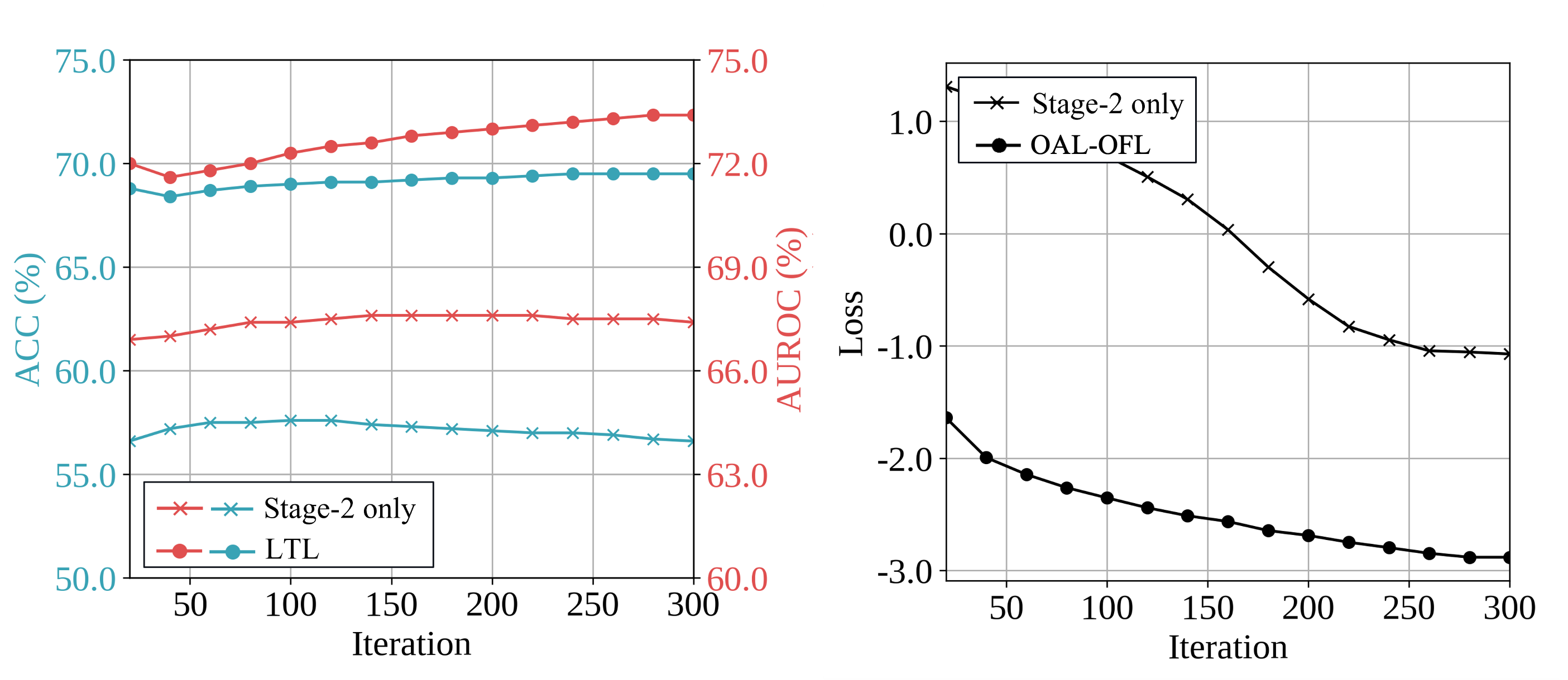
(a)

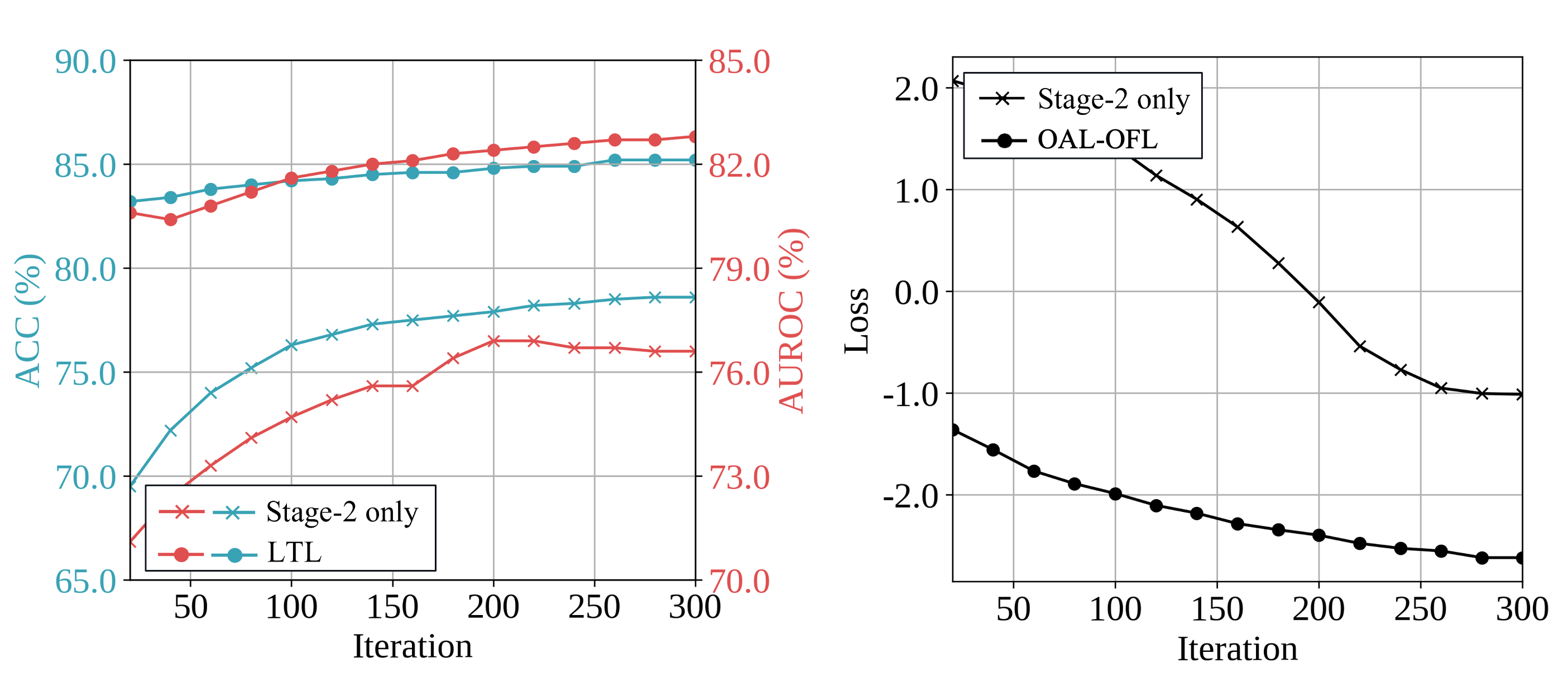
(b)

Figure 4: Plots of OAL-OFL on Acc (%), AUROC (%), and loss (logarithmic scale) on iterations in Stage-2 (Best viewed in color).

Stage-1 to prevent overfitting. Fig. 4 visualizes the changes of Acc, AUROC, and loss values during Stage-2 training. To see the impact of Stage-1 on Stage-2, we plot ‘Stage-2 only’ and our complete OAL-OFL. Fig. 4(a) right shows the loss curves. OAL-OFL starts from a pretty lower loss than ‘Stage-2 only.’ And both ‘Stage-2 only’ and OAL-OFL converge, but ‘Stage-2 only’ is saturated at a higher loss. Also, OAL-OFL shows better performance over all the iterations in the testing ACC and AUROC of Fig. 4(a) left. We can see a similar trend in 5-shot. From this result, we can infer that our Stage-1 can provide a favorable starting point, while mitigating the overfitting problem of FSOSR transfer learning.

Table 4: Ablation analysis for Stage-1.

		1-shot			5-shot
$\mathcal{L}_{\textrm{mask}}^{1}$	$(a,b)$	Acc.	AUROC		Acc.	AUROC
		66.07	70.72		82.01	80.14
$\checkmark$		66.45	71.06		81.75	80.31
$\checkmark$	$\checkmark$	67.95	71.81		82.76	80.91

Analysis on Stage-1. We exploited the scalar factors, $a$ and $b$, and masked loss $L_{\textrm{mask}}$ to facilitate learning task-independent open-set prototype in the meta-learning of Stage-1. Table 4 ablates these components. All the components are useful, and the degraded performance in the ablated ones means the difficulty of meta-learning the task-independent open-set prototype.

Table 5: Impact of the base training dataset varying the number of classes in Stage-2.

	1-shot			5-shot
#Base categories	Acc.	AUROC		Acc.	AUROC
0 (OAL-OFL-Lite)	69.15	72.71		85.61	81.11
1	66.41	69.62		83.66	79.62
6	66.72	69.71		83.15	78.34
32	68.30	71.84		84.51	81.34
64 (OAL-OFL)	69.78	73.88		85.49	83.13

Amount of $\mathcal{D}_{\mathrm{bs}}$ in Stage-2. In Table 5, we identify the impact of the variety of categories in $\mathcal{D}_{\mathrm{bs}}$ on the quality of the OFL. By reducing the number of categories in $\mathcal{D}_{\mathrm{bs}}$, the overall results are degraded. Rather, when the number of the base categories is lower than the half, OAL-OFL-Lite shows better results. Hence, it is crucial to configure the open-set training dataset from diverse base categories.

Table 6: Effect of meta-learning on the classifier of Stage-2. (Rand: random, Meta: Stage-1 meta-learned).

	Classifier initialization		1-shot			5-shot
	$\{w_{n}\}_{n=1}^{N}$	$w_{N+1}$	Acc.	AUROC		Acc.	AUROC
OAL-OFL-Lite	Rand	Rand	40.34	35.29		50.90	27.19
	Meta	Rand	57.72	68.13		78.43	79.36
	Meta	Meta	69.15	72.71		85.61	81.11
OAL-OFL	Rand	Rand	63.03	67.52		79.97	75.95
	Meta	Rand	69.02	70.87		85.32	78.50
	Meta	Meta	69.78	73.88		85.49	83.13

Meta-learned classifier. In OAL-OFL and OAL-OFL-Lite, we utilize the meta-learned feature encoder and open-set prototype to initialize the closed-set and open-set classifiers. As in Table 6, although the feature encoder starts from the meta-learned weights, the transfer-learned model suffers from severe performance degradation due to random initialization of both open and closed-set classifiers (Rand-Rand in Table 6). In OAL-OFL, when the closed-set classifiers are initialized by the class-wise prototypes from the meta-learned encoder (Meta-Rand), the closed-set classification Acc is recovered, but open-set AUROC is not. In OAL-OFL-Lite, both Acc and AUROC are quite lower than the case of complete meta-learned weight initialization. Further, when both closed and open-set classifiers are not initialized by the meta-learned weight, the open-set recognition ability of OAL-OFL is worse than OAL-OFL-Lite where classifiers are initialized by the meta-learned weights. Hence, the open-set aware meta-learning is crucial for the both closed- and open-set classifiers.

Classifier design in Stage-2. Stage-1 is based on the squared Euclidean distance as the distance metric. In order to maintain consistency in the metric space, we compute the classifier outputs under the same metric in Stage-2 of OAL-OFL. In Table 7, we compared our Euclidean classifier with the linear classifier, meaning the significance of metric-space consistency for the collaborative use of the different two learning approaches.

Cost for Stage-2. As mentioned in Sec. 4.1, we train the model with 20,000 tasks, an iteration per task in Stage-1. This is de facto standard in FSOSR methods. In our Stage-2 of both OAL-OFL and OAL-OFL-Lite, the model is further learned during 300 iterations. It is only 1.5% of Stage-1. While the model is not more generalized in Stage-1 with the 1.5% additional iterations, our Stage-2 yields notable improvement as in Table 10 through a tiny extra training cost.

Table 7: Linear vs Euclidean classifiers in OFL.

	1-shot			5-shot
Classifier	Acc.	AUROC		Acc.	AUROC
Linear	68.01	72.79		84.72	81.03
Euclidean (Ours)	69.78	73.88		85.49	83.13

5 Conclusions

This work introduced the two-stage learning approach for FSOSR called open-set aware meta-learning (OAL) on a base dataset and open-set free transfer learning (OFL) on testing tasks. Our findings highlight the significance of the meta-learned FSOSR metric space, which serves as a general starting point in transfer learning and enables us to take advantage of transfer learning. For the open-set free transfer learning, we provided two suggestions to configure open-set training data: 1) sampling from the base dataset, and 2) sampling from the testing task itself. The latter one considers a more practical scenario, not relying on the base dataset during inference. Both are beneficial for generalizing the model to an FSOSR testing task. As a result, we achieved SOTA performance on two benchmark datasets, namely miniImageNet and tieredImageNet.

6 Analysis on OAL-OFL-Lite varying iterations

Fig. 5 plots the AUROC, ACC, and loss curves for the proposed OAL-OFL-Lite framework compared to its Stage-2 (open-set free transfer learning) only version. These metrics are plotted over training iteration on the miniImageNet dataset. We can identify that the open-set aware meta-learning plays a crucial role in preventing overfitting and enhancing the efficacy of transfer learning in OAL-OFL-Lite as its impact in OAL-OFL.

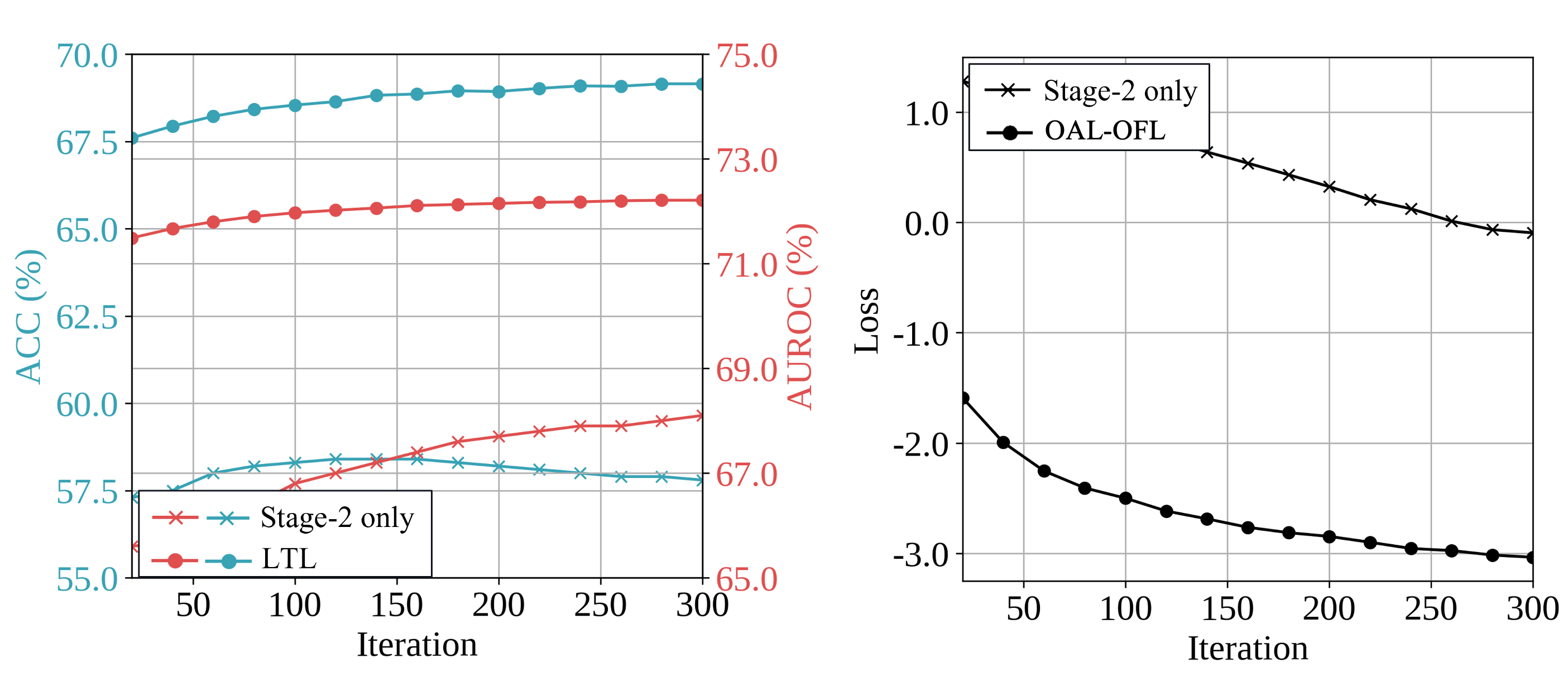
(a)

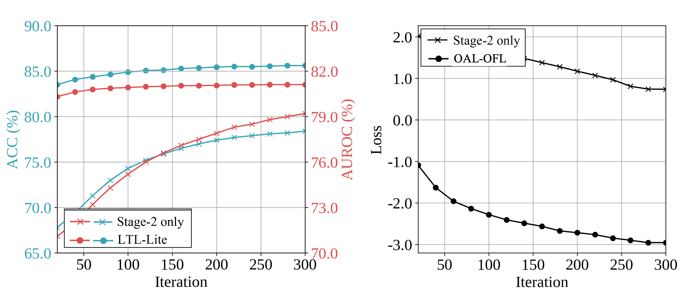
(b)

Figure 5: Plots of OAL-OFL-Lite on accuracy (%), AUROC (%), and loss (logarithmic scale) increasing iterations in Stage-2 on the 5-way 1- and 5-shot settings of the miniImageNet.

7 Threshold-free open-set detection

To evaluate the performance of open-set recognition, we utilized the widely-used AUROC metric, which is valued for its threshold-free nature. However, the task-specific adjustment of the threshold values for the detection of unseen (open-set) sample poses practical challenge in real-world scenarios.

In our research, the OAL-OFL yields a dedicated open-set classifier. This allows us to exploit the possibility associated with open-set classification for detecting open-set instances. Consequently, a feasible method for setting a threshold involves classifying an input as open-set if its probability of being an open-set class exceeds that of being closed-set classes.

Aligning with our concern, Jeong et al. [16] proposed a distinctive approach. They primarily utilized the distance between the average of prototypes and the farthest prototype to differentiate between the closed and open-set data. We conducted a comparative analysis of their results with our OAL-OFL and OAL-OFL-Lite in the context of threshold-free open-set detection in Table 8. The results highlight the effectiveness of our proposed method in detecting open-set instances without the need of any manually selected threshold, thereby underlining its practical utility and effectiveness.

Table 8: Open-set detection on 600 testing tasks of tieredImageNet 5-way 5-shot setting

Method	Accuracy (%)	F1-score	AUROC (%)
SnaTCHer-F [16]	55.44	0.6904	82.02
SnaTCHer-T [16]	54.42	0.6865	82.03
SnaTCHer-L [16]	70.82	0.7376	80.81
OAL-OFL	74.91	0.7697	83.36
OAL-OFL-Lite	73.66	0.7530	82.22

(a)

(b)

(c)

Figure 6: Distribution of the classification probabilities of closed-set and open-set queries to the open-set class. Closed-set and open-set queries are represented in green and red, respectively.

8 The Distribution of classification probability assigned to the open-set class

In Fig. 6, we present a visualization of the distributions of classification probability towards the open-set class, derived from both closed-set and open-set queries. The visualization reveals that, in the scenario labeled as ‘Stage-2 only,’ where the open-set aware meta-learning is absent, a majority of the queries are assigned high probabilities of belonging to the open-set, irrespective of their actual membership to the closed or open set. Converserly, in ‘Stage-1 only’ scenario, a significant number of closed-set queries are still attributed probabilities exceeding 0.5. On the other hand, in OAL-OFL, it is observed that the majority of open-set queries attain significantly high probabilities of being classified as the open-set, while the probabilities for closed-set queries are effectively suppressed. This distinct separation in the classification probabilities for open and closed-set queries allows us to understand and verify the robustness of OAL-OFL in effectively dichotomizing between open and closed sets.

Table 9: Training details.

	Stage-1	Stage-2
Optimizer	SGD	SGD
Optimizer momentum	0.9	0.9
Weight decay	5e-4	5e-4
Learning rate (LR)	2e-4 for $f_{\theta}$,	2e-4 for $f_{\theta}$,
	2e-5 for others	2e-3 (OAL-OFL)	for others
		2e-4 (OAL-OFL-Lite)
LR decaying	multi. 0.5	None
	every 40 episodes
$\#$ of episodes (iterations)	20,000	300

Table 10: Ablation analysis on stages in the proposed OAL-OFL on the tieredImageNet. Accuracy (%) and AUROC (%) are reported on the 5-way 1- and 5-shot settings.

Stage-1	Stage-2	1-shot			5-shot
		Acc.	AUROC		Acc.	AUROC
	$\checkmark$	64.73	70.98		83.68	80.21
$\checkmark$		70.96	75.05		84.78	82.08
$\checkmark$	$\checkmark$	71.40	75.45		86.75	83.36

Table 11: Ablation analysis for the proposed OAL-OFL-Lite in Stage-2 on the tieredImageNet. Accuracy (%) and AUROC (%) are reported on the 5-way 1- and 5-shot settings.

		1-shot			5-shot
		Acc.	AUROC		Acc.	AUROC
Naive TL to closed set		71.36	58.67		86.78	61.85
Stage-2 only		65.07	68.70		85.03	77.67
OAL-OFL-Lite		70.80	73.67		86.66	82.22
Pseudo open-set	Freeze $w_{N+1}$
		70.59	72.84		85.51	80.33
$\checkmark$		70.51	73.24		86.45	81.92
$\checkmark$	$\checkmark$	70.80	73.67		86.66	82.22

9 More details

Pretrain encoder. In alignment with the latest developments in few-shot classification and FSOSR methods [17, 16, 15], we have pre-trained the encoder, denoted as $f_{\theta}$. This was achieved using a linear classifier that categorizes all classes in the dataset $\mathcal{D}_{\text{bs}}$. The training process spanned 500 epochs utilizing the SGD optimizer. We employed cross-entropy loss complemented by self-knowledge distillation [12], and integrated rotation as per [15]. Additionally, data augmentation was implemented using the mixup [44]. This training approach aligns our work with the SOTA methods [15, 41] in the field, facilitating fair and relevant comparisons.

Additionally, the specifics of the training setup for both Stage-1 and Stage-2 of our methodologies are detiled in Table 9.

10 Ablation experiments on tieredImageNet

We conducted ablation studies for both OAL-OFL and OAL-OFL-Lite on tieredImageNet dataset. The results are presented in Tables 10 and 11, respectively.

References

- [1] Abhijit Bendale and Terrance E. Boult. Towards open set deep networks. In CVPR, 2016.
- [2] Enrique Castillo. Extreme value theory in engineering. Elsevier, 2012.
- [3] Guangyao Chen, Peixi Peng, Xiangqian Wang, and Yonghong Tian. Adversarial reciprocal points learning for open set recognition. IEEE Trans. Pattern Anal. Mach. Intell., 44(11):8065–8081, 2022.
- [4] Wei-Yu Chen, Yen-Cheng Liu, Zsolt Kira, Yu-Chiang Frank Wang, and Jia-Bin Huang. A closer look at few-shot classification. In ICLR, 2019.
- [5] Jesse Davis and Mark Goadrich. The relationship between precision-recall and ROC curves. In ICML, 2006.
- [6] Jacob Devlin, Ming-Wei Chang, Kenton Lee, and Kristina Toutanova. BERT: pre-training of deep bidirectional transformers for language understanding. In NAACL, 2019.
- [7] Jeff Donahue, Yangqing Jia, Oriol Vinyals, Judy Hoffman, Ning Zhang, Eric Tzeng, and Trevor Darrell. Decaf: A deep convolutional activation feature for generic visual recognition. In ICML, 2014.
- [8] Tom Fawcett. An introduction to ROC analysis. Pattern Recognition Letters, 27(8):861–874, 2006.
- [9] Li Fei-Fei, Robert Fergus, and Pietro Perona. One-shot learning of object categories. IEEE Trans. Pattern Anal. Mach. Intell., 28(4):594–611, 2006.
- [10] Chelsea Finn, Pieter Abbeel, and Sergey Levine. Model-agnostic meta-learning for fast adaptation of deep networks. In ICML, 2017.
- [11] Chelsea Finn, Kelvin Xu, and Sergey Levine. Probabilistic model-agnostic meta-learning. In NeurIPS, 2018.
- [12] Tommaso Furlanello, Zachary Lipton, Michael Tschannen, Laurent Itti, and Anima Anandkumar. Born again neural networks. In ICLR, 2018.
- [13] Zongyuan Ge, Sergey Demyanov, and Rahil Garnavi. Generative openmax for multi-class open set classification. In BMVC, 2017.
- [14] Kaiming He, Xiangyu Zhang, Shaoqing Ren, and Jian Sun. Deep residual learning for image recognition. In CVPR, 2016.
- [15] Shiyuan Huang, Jiawei Ma, Guangxing Han, and Shih-Fu Chang. Task-adaptive negative envision for few-shot open-set recognition. In CVPR, 2022.
- [16] Minki Jeong, Seokeon Choi, and Changick Kim. Few-shot open-set recognition by transformation consistency. In CVPR, 2021.
- [17] Yiren Jian and Lorenzo Torresani. Label hallucination for few-shot classification. In AAAI, 2022.
- [18] Pedro Ribeiro Mendes Júnior, Roberto Medeiros de Souza, Rafael de Oliveira Werneck, Bernardo V. Stein, Daniel V. Pazinato, Waldir R. de Almeida, Otávio A. B. Penatti, Ricardo da Silva Torres, and Anderson Rocha. Nearest neighbors distance ratio open-set classifier. Machine Learning, 106(3):359–386, 2017.
- [19] Byeonggeun Kim, Seunghan Yang, Inseop Chung, and Simyung Chang. Dummy prototypical networks for few-shot open-set keyword spotting. In Interspeech, 2022.
- [20] Duong H. Le, Khoi D. Nguyen, Khoi Nguyen, Quoc-Huy Tran, Rang Nguyen, and Binh-Son Hua. POODLE: improving few-shot learning via penalizing out-of-distribution samples. In NeurIPS, 2021.
- [21] Kwonjoon Lee, Subhransu Maji, Avinash Ravichandran, and Stefano Soatto. Meta-learning with differentiable convex optimization. In CVPR, 2019.
- [22] Yoonho Lee and Seungjin Choi. Gradient-based meta-learning with learned layerwise metric and subspace. In ICML, 2018.
- [23] Shiyu Liang, Yixuan Li, and R. Srikant. Enhancing the reliability of out-of-distribution image detection in neural networks. In ICLR, 2018.
- [24] Bo Liu, Hao Kang, Haoxiang Li, Gang Hua, and Nuno Vasconcelos. Few-shot open-set recognition using meta-learning. In CVPR, 2020.
- [25] Marc Masana, Idoia Ruiz, Joan Serrat, Joost van de Weijer, and Antonio M. López. Metric learning for novelty and anomaly detection. In BMVC, 2018.
- [26] Yurii E Nesterov. A method for solving the convex programming problem with convergence rate O (1/k^ 2). In Dokl. akad. nauk Sssr, volume 269, pages 543–547, 1983.
- [27] Alex Nichol, Joshua Achiam, and John Schulman. On first-order meta-learning algorithms. CoRR, abs/1803.02999, 2018.
- [28] Poojan Oza and Vishal M. Patel. C2AE: class conditioned auto-encoder for open-set recognition. In CVPR, 2019.
- [29] Pramuditha Perera, Vlad I. Morariu, Rajiv Jain, Varun Manjunatha, Curtis Wigington, Vicente Ordonez, and Vishal M. Patel. Generative-discriminative feature representations for open-set recognition. In CVPR, 2020.
- [30] Alec Radford, Karthik Narasimhan, Tim Salimans, Ilya Sutskever, et al. Improving language understanding by generative pre-training. OpenAI, 2018.
- [31] Jathushan Rajasegaran, Salman Khan, Munawar Hayat, Fahad Shahbaz Khan, and Mubarak Shah. Self-supervised knowledge distillation for few-shot learning. In BMVC, 2021.
- [32] Sachin Ravi and Hugo Larochelle. Optimization as a model for few-shot learning. In ICLR, 2017.
- [33] Mengye Ren, Eleni Triantafillou, Sachin Ravi, Jake Snell, Kevin Swersky, Joshua B. Tenenbaum, Hugo Larochelle, and Richard S. Zemel. Meta-learning for semi-supervised few-shot classification. In ICLR, 2018.
- [34] Mamshad Nayeem Rizve, Salman Khan, Fahad Shahbaz Khan, and Mubarak Shah. Exploring complementary strengths of invariant and equivariant representations for few-shot learning. In CVPR, 2021.
- [35] Aniket Roy, Anshul Shah, Ketul Shah, Prithviraj Dhar, Anoop Cherian, and Rama Chellappa. Felmi: Few shot learning with hard mixup. In NeurIPS, 2022.
- [36] Richard L Smith. Extreme value theory. Handbook of applicable mathematics, 7(437-471):18, 1990.
- [37] Jake Snell, Kevin Swersky, and Richard S. Zemel. Prototypical networks for few-shot learning. In NeurIPS, 2017.
- [38] Xin Sun, Zhenning Yang, Chi Zhang, Keck Voon Ling, and Guohao Peng. Conditional gaussian distribution learning for open set recognition. In CVPR, 2020.
- [39] Yonglong Tian, Yue Wang, Dilip Krishnan, Joshua B Tenenbaum, and Phillip Isola. Rethinking few-shot image classification: a good embedding is all you need. In ECCV, 2020.
- [40] Oriol Vinyals, Charles Blundell, Tim Lillicrap, Koray Kavukcuoglu, and Daan Wierstra. Matching networks for one shot learning. In NeurIPS, 2016.
- [41] Haoyu Wang, Guansong Pang, Peng Wang, Lei Zhang, Wei Wei, and Yanning Zhang. Glocal energy-based learning for few-shot open-set recognition. In CVPR, 2023.
- [42] Han-Jia Ye, Hexiang Hu, De-Chuan Zhan, and Fei Sha. Few-shot learning via embedding adaptation with set-to-set functions. In CVPR, 2020.
- [43] Ryota Yoshihashi, Wen Shao, Rei Kawakami, Shaodi You, Makoto Iida, and Takeshi Naemura. Classification-reconstruction learning for open-set recognition. In CVPR, 2019.
- [44] Hongyi Zhang, Moustapha Cissé, Yann N. Dauphin, and David Lopez-Paz. mixup: Beyond empirical risk minimization. In ICLR, 2018.
- [45] Da-Wei Zhou, Han-Jia Ye, and De-Chuan Zhan. Learning placeholders for open-set recognition. In CVPR, 2021.