Virtual entanglement purification via noisy entanglement
Kaoru Yamamoto
kaoru.yamamoto@ntt.comNTT Computer and Data Science Laboratories, NTT Corporation, Musashino 180-8585, Japan
Yuichiro Matsuzaki
Department of Electrical, Electronic, and Communication Engineering, Faculty of Science and Engineering, Chuo University, 1-13-27 Kasuga, Bunkyo-ku, Tokyo 112-8551, Japan
Yasunari Suzuki
NTT Computer and Data Science Laboratories, NTT Corporation, Musashino 180-8585, Japan
Yuuki Tokunaga
NTT Computer and Data Science Laboratories, NTT Corporation, Musashino 180-8585, Japan
Suguru Endo
suguru.endou@ntt.comNTT Computer and Data Science Laboratories, NTT Corporation, Musashino 180-8585, Japan
JST, PRESTO, 4-1-8 Honcho, Kawaguchi, Saitama, 332-0012, Japan
Abstract
Distributed quantum computation (DQC) offers a promising approach for scalable quantum computing, where high-fidelity non-local operations among remote devices are required for universal quantum computation.
These operations are typically implemented through teleportation, which consumes high-fidelity entanglement prepared via entanglement purification.
However, noisy local operations and classical communication (LOCC) limit the fidelity of purified entanglement, thereby degrading the quality of non-local operations.
Here, we present a protocol utilizing virtual operations that purifies noisy entanglement at the level of expectation values.
Our protocol offers the following advantages over conventional methods: surpassing the fidelity limit of entanglement purification in the presence of noise in LOCC, requiring fewer sampling shots than circuit knitting, and exhibiting robustness against infidelity fluctuations in shared noisy Bell states unlike probabilistic error cancellation.
Our protocol bridges the gap between DQC with entanglement and with circuit knitting, thus providing a flexible way for further scalability in the presence of hardware limitations.
Introduction.–
Quantum computers promise to outperform classical computers in computational power, which requires many physical qubits for fault-tolerant computation.
Although current technological advancements have increased the number of qubits on a single quantum processing unit (QPU), further scalability is crucial for achieving quantum supremacy.
A promising approach for this scalability is distributed quantum computation (DQC) with a modular architecture, which requires high-fidelity entanglement generation and non-local operations among remote QPUs Cabrillo et al. (1999); Bose et al. (1999); Benjamin et al. (2005); Chou et al. (2005); Lim et al. (2005); Barrett and Kok (2005); Benjamin et al. (2006); Moehring et al. (2007); Benjamin et al. (2009); Nickerson et al. (2014); Nigmatullin et al. (2016); Bravyi et al. (2022); Ang et al. (2022); Jnane et al. (2022).
However, non-local operations realized in the current experiment are still noisy Kurpiers et al. (2018); Chou et al. (2018); Campagne-Ibarcq et al. (2018); Zhong et al. (2019); Kannan et al. (2020); Zhong et al. (2021); Daiss et al. (2021); van Leent et al. (2022); Luo et al. (2022); Leung et al. (2019); Yan et al. (2022); Chan et al. (2023); Qiu et al. (2023); Grebel et al. (2024).
Alternatively, circuit knitting (and cutting), which simulates non-local operations by employing separable state preparation along with local operations and classical communication (LOCC), has been considered for DQC Piveteau and Sutter (2023); Bäumer et al. (2023); Vazquez et al. (2024); Jin et al. (2024).
Nonetheless, this approach requires excessive additional circuit runs and is impractical for further scalability.
A typical approach for realizing high-fidelity non-local operations is to utilize entanglement purification Bennett et al. (1996a); Deutsch et al. (1996); Dür and Briegel (2007); Fujii and Yamamoto (2009); Krastanov et al. (2019); Riera-Sàbat et al. (2021a); Krastanov et al. (2021); Goodenough et al. (2024): remote QPUs share noisy entanglement, generate high-fidelity entanglement from them by entanglement purification and then consume the purified entanglement for state and gate teleportations with LOCC Bennett et al. (1993); Eisert et al. (2000); Pirandola et al. (2015); Hu et al. (2023); Wu et al. (2023).
Entanglement purification has been considered to be promising for realizing high-fidelity non-local operations.
However, local noise in a QPU limits the maximal achievable fidelity of purified entanglement Fujii and Yamamoto (2009); Krastanov et al. (2019).
For example, the order of 1% two-qubit gate error rate in a local QPU, which can be achieved in current integrated quantum computers Kim et al. (2023), limits the minimum achievable infidelity to the order of 0.5% Fujii and Yamamoto (2009); Krastanov et al. (2019).
This may not be sufficient for practical large-scale quantum computation in an error-corrected regime.
Researchers have investigated more efficient protocols even with hardware limitations and imperfections Fujii and Yamamoto (2009); Krastanov et al. (2019); Riera-Sàbat et al. (2021a); Krastanov et al. (2021); Goodenough et al. (2024).
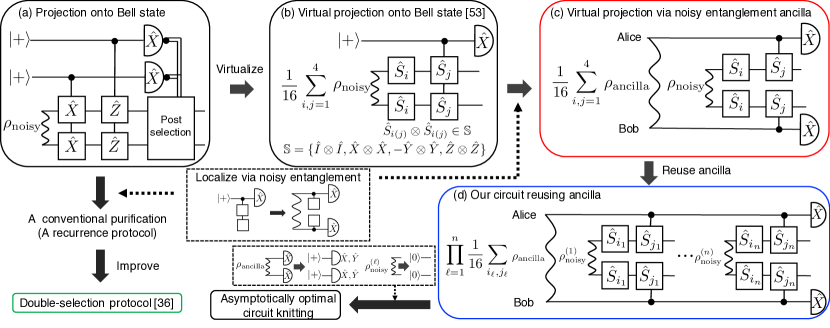
Figure 1: Schematics of the overview and construction of our virtual circuit. (a) Purification with Bell-state projection by indirect measurement and post-selection, which is the origin of our virtual circuit as well as the conventional double-selection protocol Fujii and Yamamoto (2009).
(b) Virtual purification with Bell-state projection including non-local controlled operations.
(c) Our virtual purification circuit with noisy-entanglement preparation and local-controlled operation.
(d) Our circuit with ancilla reuse. Moreover, replacing all entanglement states with suitable separable states and additional measurements on the ancilla as shown provides the circuit of asymptotically optimal circuit knitting.
To overcome this fidelity limitation, we leverage the concept of virtual operations, mainly developed within the field of quantum error mitigation (QEM) Endo et al. (2021); Cai et al. (2023).
Virtual operations mitigate errors at the expectation value level rather than in a quantum state itself by classically post-processing outputs from additional circuit runs.
Here, we propose a virtual entanglement purification protocol via noisy-entanglement preparation by utilizing virtual operations confined to LOCC. Such virtually purified entanglement can be used for state and gate teleportations to realize high-fidelity non-local operations.
Our demonstration shows the corresponding advantages over conventional entanglement purification, circuit knitting, and probabilistic error cancellation (PEC) for noisy Bell states Yuan et al. (2024); Zhang et al. (2023); Takagi et al. (2024).
Our protocol produces purified Bell states with a leading-order infidelity term of , where and are a local two-qubit gate error rate and the infidelity of initial noisy Bell states, respectively.
Remarkably, this breaks the fidelity limit of conventional protocols, Fujii and Yamamoto (2009); Krastanov et al. (2019).
Moreover, our protocol achieves much lower sampling overhead than circuit knitting by utilizing noisy entanglement as a resource: compared with the optimal circuit knitting, a noisy Bell state with 10% infidelity reduces the sampling overhead by around for simulating purified Bell states.
Finally, we demonstrate the robustness of our protocol against infidelity fluctuations in shared noisy Bell states unlike PEC Yuan et al. (2024); Zhang et al. (2023); Takagi et al. (2024), coming from the error-agnostic property of our protocol.
Our proposed protocol bridges the gap between DQC with entanglement and with circuit knitting, thus providing a flexible way for further scalability in the presence of hardware limitations.
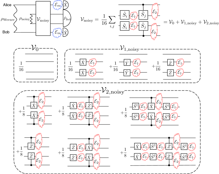
Virtual entanglement purification.–
To explain our quantum circuit, we start from a quantum circuit in Fig. 1(a).
This circuit projects the input noisy state, , onto the Bell state, , by indirectly measuring the stabilizer generators of the Bell states, and , and then post-selecting the target state depending on the measurement results.
This implements projection onto the Bell state, Nielsen and Chuang (2002); Tsubouchi et al. (2023).
Note that replacing the non-local controlled operations in Fig. 1(a) with noisy-entanglement preparation and local controlled operations, this circuit becomes a conventional purification circuit classified as a recurrence protocol, and its improved version is the double-selection protocol Fujii and Yamamoto (2009).
Tsubouchi et al. recently introduced virtual projection onto the stabilizer space Tsubouchi et al. (2023).
Taking the projection onto the Bell state as an example, their idea is to decompose the projector into the sum of its stabilizers as with and implementing Monte-Carlo sampling to estimate each term in as follows.
Suppose we want to estimate the expectation value of an observable for the projected state after applying a completely positive trace-preserving (CPTP) map .
The expectation value from measuring on shown in Fig. 1(b) and on the target state after applying the CPTP map is .
Additionally, we can simultaneously estimate by disregarding the measurement of , as part of the same experimental setup.
The desired expectation value, , is obtained by dividing the averages of these expectation values over the stabilizer group as
(1)
where we used .
In this way, as long as we want the expectation value, we can treat (virtually) purified states as real purified states with conventional purification.
Our idea is to implement this virtual projection by replacing the non-local controlled operation in Fig. 1(b) with the noisy-entanglement ancilla state and local controlled operations for DQC (Fig. 1)(c).
If we could prepare the Bell state ancilla, we could implement the same procedure above by replacing the measurement on the in Fig. 1(b) with measurement on in Fig. 1(c).
Although we can prepare only a noisy entangled state in DQC, we find that some kinds of noisy entangled states, including a Werner state or a Bell state with amplitude damping or dephasing noise, only reduce the expectation value with a constant factor, as shown in Supplementary Materials (SM) sup , and we can obtain the desired expectation value since this factor vanishes by the division in Eq. (1).
Indeed, this can be seen as a virtual version of conventional recurrence protocols Bennett et al. (1996a, b); Fujii and Yamamoto (2009); Dür and Briegel (2007); Krastanov et al. (2019) due to its construction; see Fig. 1.
For general settings, suppose we want to implement a quantum computation that outputs , where is a local operator, is a CPTP map including non-local two-qubit operations acting on some input state .
In DQC, these non-local operations are realized by state and gate teleportations consuming Bell states, and the desired expectation value is , where is a CPTP operation including teleportations that consumes , although we can only prepare noisy Bell states in typical DQC.
Our protocol described below provides the desired expectation value by virtually purifying noisy Bell states, with being the -th noisy state, using additional noisy entangled ancilla state.
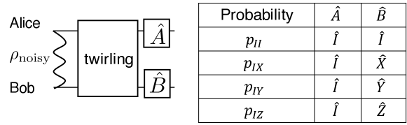
To ensure the generality of our protocol, we use a Werner state with an infidelity as an entangled ancilla state, , because this state can be prepared from any two-qubit state without changing its fidelity by suitable twirling operations Bennett et al. (1996b).
The complete protocol is as follows:
1.
In preparation for -th circuit run, Alice and Bob share noisy Bell states and make Werner states by twirling noisy Bell states out of .
They uniformly sample the indices with for purifying -th noisy Bell state and share them by classical communication.
2.
They run the quantum circuit for an input state, , where they use purification circuit in Fig. 1(c) to generate (virtually) purified Bell states and consume them for non-local two-qubit operations.
3.
They classically communicate their measurement results and record the results of as and as , where denotes the measurement on the -th Werner state ancilla.
4.
They repeat the procedures above times and calculate their averages as and .
5.
Output , which provides the desired expectation value of as
(2)
where is the projector on the ideal Bell state for -th noisy state.
Since the division by , which is an estimator of with being a infidelity of the -th Werner state ancilla, increases the variance of by , we need more sampling of the noisy circuit run Endo et al. (2022); Tsubouchi et al. (2023), where
(3)
is the sampling-cost factor with being the fidelity of the -th noisy state.
Instead of Werner states, we can repeatedly use only one Werner ancilla state as shown in Fig. 1(d).
This reduces the sampling-cost factor as with being the infidelity of a Werner state ancilla, and therefore more efficient if we can neglect temporal decoherence i.e. for sufficiently short ancilla reuse times.
Moreover, as we will discuss later, replacing all entanglement states with suitable separable states and additional measurements produces an asymptotically optimal circuit knitting circuit.
Comparison with conventional purification.–
The performance of conventional entanglement purification protocols is evaluated using the quantity called yield defined as the ratio between the number of purified and noisy Bell states with its fidelity being and , respectively.
The yield can be written as ,
where is the number of purification rounds required to achieve , is the number of noisy Bell states consumed for the -th round.
Here, is the success probability of the -th purification round using the -th noisy Bell states with a fidelity of , where Dür and Briegel (2007); Fujii and Yamamoto (2009); Riera-Sàbat et al. (2021a, b).
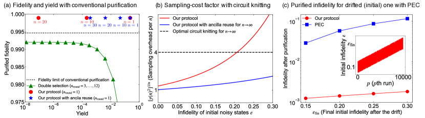
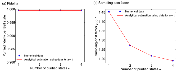
Figure 2: (a) Purified fidelity with the corresponding yield for our protocol with and without the ancilla reuse (the blue stars and red circles, respectively) and conventional double-selection protocol (the green curve with triangles).
The black dotted line shows the upper limit of the fidelity achievable by conventional protocols Fujii and Yamamoto (2009); Krastanov et al. (2019). We consider the geometric-mean fidelity for multiple .
(b) Sampling overhead per purified Bell state, , with the initial infidelity of the input noisy states and Werner ancilla states for our protocol.
The black dotted horizontal lines represent the lower bounds for circuit knitting for , Piveteau and Sutter (2023); Brenner et al. (2023); Harada et al. (2024).
(c) Infidelity after purification for our protocol and a simple Pauli PEC with the noisy input state , where is the Werner state for -th run with its infidelity drifted as shown in the inset
To evaluate the performance of our virtual protocol, we extend the definition of yield for virtual purification protocols.
As virtual protocols require a sampling overhead increased by a factor of to achieve the same accuracy as that for non-virtual protocols Endo et al. (2022); Tsubouchi et al. (2023), we define the yield for our protocol as
(4)
Note that, since usual virtual protocols are constructed to obtain the expectation value of with the (virtually) purified state , the entanglement fidelity Dür and Briegel (2007); Riera-Sàbat et al. (2021b), defined as , is obtained by setting .
In this way, is calculated by implementing the Bell measurement on the (virtually) purified states in the following numerical simulation for our protocol and PEC: see also the quantum circuit in SM sup .
We numerically calculated their purified fidelity and the corresponding yield using Qulacs Suzuki et al. (2021).
For simplicity, we set with an initial fidelity of for all .
We chose the double-selection protocol Fujii and Yamamoto (2009) as a benchmark because it can be seen as the non-virtual protocol for ours (see Fig. 1).
We introduced the following local noise: single-qubit depolarizing noise after each single-qubit gate, with , two-qubit depolarizing noise after each two-qubit gate, with , and readout error before each measurement, with .
Figure 2 (a) shows the purified fidelity and the corresponding yield.
Note that we use the geometrical-mean fidelity, , as the purified fidelity for our virtual protocols.
As shown, our virtual protocol with and without the ancilla reuse achieves a fidelity of 99.9%, much higher than the maximum fidelity of the double-selection protocol.
Although the yield for our protocol exponentially decreases with increasing , it is comparable to the yield for the double-selection protocol for a few tens of .
Remarkably, the purified fidelity of our protocol also surpasses the upper fidelity limit of 99.5% for conventional protocols with Fujii and Yamamoto (2009); Krastanov et al. (2019).
This is due to the effect of local two-qubit noise on the virtual state at the expectation value level in our virtual protocol, which is different from that on the real state in conventional purification protocols.
The fidelity limit of conventional protocols comes from local two-qubit errors that cannot be detected by one-shot measurement on the ancillae.
These errors include ones that do not affect the ancillae but the target states, such as .
In addition, at least one kind of cannot be detected intrinsically; see Refs. Fujii and Yamamoto (2009); Krastanov et al. (2019) in details. Therefore, there are four errors of kinds of local two-qubit errors that cannot be detected and these errors exist for Alice and Bob, respectively, leading to an infidelity limit of Fujii and Yamamoto (2009); Krastanov et al. (2019).
Meanwhile, at the expectation value level in our protocol, the two-qubit errors only reduce the amplitude of the expectation value, and the leading-order term of vanishes due to the division in Eq. (2), resulting in purified Bell states with a leading-order infidelity term of .
A detailed analysis of this and other noises is left to SM sup .
Comparison with circuit knitting.–
Circuit knitting simulates entanglement with only separable-state preparation and LOCC, but requires more sampling to achieve the same accuracy.
To simulate Bell states using circuit knitting, we first decompose , where is a coefficient, is a CPTP map confined to LOCC, is a separable state, and is a probability distribution.
We can thus simulate by summing up the results of the outcome obtained by Monte-Carlo sampling with the probability distribution and multiplied by .
Figure 2 (b) compares the sampling overhead per Bell state, , for our protocol with that for optimal one for circuit knitting, Piveteau and Sutter (2023); Brenner et al. (2023); Harada et al. (2024).
The numerical setup including local noise is the same as that in comparison with conventional purification.
Our protocol shows a much lower sampling overhead than optimal circuit knitting for reasonable initial infidelity.
For example, a 10% infidelity of initial Werner states, which may be achievable in current technologies Chou et al. (2018); Campagne-Ibarcq et al. (2018); Kannan et al. (2020); Daiss et al. (2021); van Leent et al. (2022); Luo et al. (2022); Leung et al. (2019); Yan et al. (2022); Chan et al. (2023); Qiu et al. (2023), makes around half of that for optimal circuit knitting, leading to the reduction of the total sampling overhead by around for simulating purified Bell states.
This reduction comes from using noisy entanglement as a resource in our protocol.
Our protocol thus can be seen as an extension of circuit knitting utilizing entanglement.
We finally remark that we can produce an asymptotically optimal circuit-knitting protocol from our protocol with ancilla reuse, by implementing and measurements on ancilla instead of on a noisy entanglement ancilla as well as considering initial states as separable states such as : see Fig. 1.
As shown in SM sup , the additional measurement of doubles , and the fidelity of to is , leading to .
Using this approach, we can construct an asymptotically optimal circuit-knitting protocol that inherits the noise-resilient properties of our original protocol.
Robustness to the drift in initial-state infidelity.–
Our protocol is robust to the drift of initial infidelity because it effectively projects the state onto the symmetric subspace for the stabilizers .
Denote the -th initial noisy state in the -th experimental run as and the total number of experimental runs as .
The expectation value in the presence of the drifted noise can be described as
(5)
where .
This implies that our virtual protocol works for the averaged state .
Using this average state, we conducted a numerical experiment for our protocol and a simple Pauli PEC, which requires error information; see details for this PEC in SM sup .
For numerical demonstration, we have the initial infidelity drift from to as with uniform random fluctuation between , while the estimated for PEC is assumed to be ; see the inset to Fig. 2(c).
We use the same noise as that for comparison with conventional purification.
With these parameters, we construct the initial average noisy state with and calculate the purified infidelity for our protocol and the PEC, respectively, as shown in Fig. 2(c).
As shown, our protocol shows much better robustness to the drift in initial infidelity than PEC.
Conclusion and outlook.–
We have proposed a virtual entanglement purification protocol for DQC that purifies noisy Bell states at the expectation value level.
We have demonstrated corresponding advantages compared to conventional entanglement purification, circuit knitting, and PEC for noisy Bell states: surpassing the fidelity limit in the presence of noise in LOCC, requiring fewer sampling shots, and exhibiting robustness against initial infidelity fluctuations in shared entanglement.
As a byproduct, we have also proposed an asymptotically optimal circuit-knitting protocol that may inherit the noise-resilient properties of our original protocol.
Our protocol bridges the gap between entanglement purification and circuit knitting, thus providing a flexible way for DQC.
We may combine virtual purification flexibly with conventional entanglement purification and other error mitigation techniques.
Future work includes the extension of our virtual protocol for multiple entangled states such as the GHZ and linear cluster states.
Moreover, replacing non-local controlled operations with noisy entanglement preparation and local controlled operations can be applied to the generalized Hadamard test as shown in SM sup .
Since the Hadamard test is a building block for many error mitigation protocols or quantum computation algorithms Lin and Tong (2022) including the single-ancilla linear combination of unitaries Chakraborty (2023), this replacement may be useful in applying such protocols or algorithms for DQC, where operations are constrained to LOCC.
Acknowledgements.
Acknowledgments.—
This work was supported by JST [Moonshot R&D] Grant Nos. JPMJMS2061 and JPMJMS226C; JST, PRESTO, Grant No. JPMJPR2114, Japan; MEXT Q-LEAP, Grant Nos. JPMXS0120319794 and JPMXS0118068682; JST CREST Grant No. JPMJCR23I4; JSPS KAKENHI, Grant No. 23H04390.
This work was supported by
JST Moonshot (Grant Number JPMJMS226C). Y. M. is supported by JSPS KAKENHI (Grant Number
23H04390). This work was also supported by CREST
(JPMJCR23I5), JST.
Part of numerical calculations were performed using Qulacs Suzuki et al. (2021).
References
Cabrillo et al. (1999)C. Cabrillo, J. I. Cirac,
P. García-Fernández, and P. Zoller, “Creation of entangled states of distant atoms by interference,” Phys. Rev. A 59, 1025–1033 (1999).
Bose et al. (1999)S. Bose, P. L. Knight,
M. B. Plenio, and V. Vedral, “Proposal for teleportation of an atomic
state via cavity decay,” Phys. Rev. Lett. 83, 5158–5161 (1999).
Benjamin et al. (2005)S C Benjamin, J Eisert, and T M Stace, “Optical generation of matter
qubit graph states,” New J. Phys. 7, 194 (2005).
Chou et al. (2005)C. W. Chou, H. de Riedmatten,
D. Felinto, S. V. Polyakov, S. J. van Enk, and H. J. Kimble, “Measurement-induced entanglement for excitation
stored in remote atomic ensembles,” Nature (London) 438, 828–832 (2005).
Lim et al. (2005)Yuan Liang Lim, Almut Beige, and Leong Chuan Kwek, “Repeat-until-success linear optics distributed quantum computing,” Phys. Rev. Lett. 95, 030505 (2005).
Barrett and Kok (2005)Sean D. Barrett and Pieter Kok, “Efficient
high-fidelity quantum computation using matter qubits and linear optics,” Phys. Rev. A 71, 060310 (2005).
Benjamin et al. (2006)Simon C Benjamin, Daniel E Browne, Joe Fitzsimons, and John J L Morton, “Brokered graph-state quantum computation,” New J.
Phys. 8, 141 (2006).
Moehring et al. (2007)D. L. Moehring, P. Maunz,
S. Olmschenk, K. C. Younge, D. N. Matsukevich, L. M. Duan, and C. Monroe, “Entanglement of single-atom quantum bits at a distance,” Nature (London) 449, 68–71 (2007).
Benjamin et al. (2009)S.C. Benjamin, B.W. Lovett,
and J.M. Smith, “Prospects for
measurement-based quantum computing with solid state spins,” Laser & Photonics Reviews 3, 556–574 (2009).
Nickerson et al. (2014)Naomi H. Nickerson, Joseph F. Fitzsimons, and Simon C. Benjamin, “Freely scalable quantum technologies using cells of
5-to-50 qubits with very lossy and noisy photonic links,” Phys.
Rev. X 4, 041041
(2014).
Nigmatullin et al. (2016)Ramil Nigmatullin, Christopher J Ballance, Niel de Beaudrap, and Simon C Benjamin, “Minimally complex ion traps as modules for quantum communication and
computing,” New J. Phys. 18, 103028 (2016).
Bravyi et al. (2022)Sergey Bravyi, Oliver Dial,
Jay M. Gambetta, Darío Gil, and Zaira Nazario, “The future of quantum computing with
superconducting qubits,” J. Appl. Phys. 132, 160902 (2022).
Ang et al. (2022)James Ang, Gabriella Carini,
Yanzhu Chen, Isaac Chuang, Michael Austin DeMarco, Sophia E Economou, Alec Eickbusch, Andrei Faraon, Kai-Mei Fu, Steven M Girvin, et al., “Architectures for multinode
superconducting quantum computers,” arXiv:2212.06167 (2022).
Jnane et al. (2022)Hamza Jnane, Brennan Undseth, Zhenyu Cai,
Simon C. Benjamin, and Bálint Koczor, “Multicore quantum
computing,” Phys. Rev. Appl. 18, 044064 (2022).
Kurpiers et al. (2018)P. Kurpiers, P. Magnard,
T. Walter, B. Royer, M. Pechal, J. Heinsoo, Y. Salathé, A. Akin, S. Storz, J. C. Besse,
S. Gasparinetti, A. Blais, and A. Wallraff, “Deterministic quantum state transfer and remote
entanglement using microwave photons,” Nature 558, 264–267
(2018).
Chou et al. (2018)Kevin S. Chou, Jacob Z. Blumoff, Christopher S. Wang, Philip C. Reinhold, Christopher J. Axline, Yvonne Y. Gao, L. Frunzio, M. H. Devoret, Liang Jiang,
and R. J. Schoelkopf, “Deterministic teleportation
of a quantum gate between two logical qubits,” Nature
(London) 561, 368–373
(2018).
Campagne-Ibarcq et al. (2018)P. Campagne-Ibarcq, E. Zalys-Geller, A. Narla,
S. Shankar, P. Reinhold, L. Burkhart, C. Axline, W. Pfaff, L. Frunzio, R. J. Schoelkopf, and M. H. Devoret, “Deterministic remote entanglement of superconducting circuits through
microwave two-photon transitions,” Phys. Rev. Lett. 120, 200501 (2018).
Zhong et al. (2019)Y. P. Zhong, H. S. Chang,
K. J. Satzinger, M. H. Chou, A. Bienfait, C. R. Conner, É. Dumur, J. Grebel, G. A. Peairs, R. G. Povey, D. I. Schuster, and A. N. Cleland, “Violating
bell’s inequality with remotely connected superconducting qubits,” Nat. Phys. 15, 741–744 (2019).
Kannan et al. (2020)B. Kannan, D. L. Campbell, F. Vasconcelos, R. Winik,
D. K. Kim, M. Kjaergaard, P. Krantz, A. Melville, B. M. Niedzielski, J. L. Yoder, T. P. Orlando, S. Gustavsson,
and W. D. Oliver, “Generating spatially
entangled itinerant photons with waveguide quantum electrodynamics,” Science Advances 6, eabb8780 (2020).
Zhong et al. (2021)Youpeng Zhong, Hung-Shen Chang, Audrey Bienfait, Étienne Dumur, Ming-Han Chou,
Christopher R. Conner,
Joel Grebel, Rhys G. Povey, Haoxiong Yan, David I. Schuster, and Andrew N. Cleland, “Deterministic multi-qubit entanglement in a
quantum network,” Nature (London) 590, 571–575 (2021).
Daiss et al. (2021)Severin Daiss, Stefan Langenfeld, Stephan Welte, Emanuele Distante, Philip Thomas, Lukas Hartung,
Olivier Morin, and Gerhard Rempe, “A quantum-logic gate between
distant quantum-network modules,” Science 371, 614–617 (2021).
van Leent et al. (2022)Tim van Leent, Matthias Bock, Florian Fertig,
Robert Garthoff, Sebastian Eppelt, Yiru Zhou, Pooja Malik, Matthias Seubert, Tobias Bauer, Wenjamin Rosenfeld, Wei Zhang, Christoph Becher, and Harald Weinfurter, “Entangling single atoms over 33 km telecom fibre,” Nature (London) 607, 69–73 (2022).
Luo et al. (2022)Xi-Yu Luo, Yong Yu, Jian-Long Liu, Ming-Yang Zheng, Chao-Yang Wang, Bin Wang, Jun Li, Xiao Jiang, Xiu-Ping Xie, Qiang Zhang, Xiao-Hui Bao, and Jian-Wei Pan, “Postselected entanglement
between two atomic ensembles separated by 12.5 km,” Phys. Rev. Lett. 129, 050503 (2022).
Leung et al. (2019)N. Leung, Y. Lu, S. Chakram, R. K. Naik, N. Earnest, R. Ma, K. Jacobs, A. N. Cleland,
and D. I. Schuster, “Deterministic bidirectional
communication and remote entanglement generation between superconducting
qubits,” npj Quantum Information 5, 18 (2019).
Yan et al. (2022)Haoxiong Yan, Youpeng Zhong, Hung-Shen Chang, Audrey Bienfait, Ming-Han Chou, Christopher R. Conner, Étienne Dumur, Joel Grebel,
Rhys G. Povey, and Andrew N. Cleland, “Entanglement purification
and protection in a superconducting quantum network,” Phys. Rev. Lett. 128, 080504 (2022).
Chan et al. (2023)Ming Lai Chan, Alexey Tiranov, Martin Hayhurst Appel, Ying Wang,
Leonardo Midolo, Sven Scholz, Andreas D. Wieck, Arne Ludwig, Anders Søndberg Sørensen, and Peter Lodahl, “On-chip spin-photon entanglement based
on photon-scattering of a quantum dot,” npj
Quantum Information 9, 49 (2023).
Qiu et al. (2023)Jiawei Qiu, Yang Liu,
Jingjing Niu, Ling Hu, Yukai Wu, Libo Zhang, Wenhui Huang, Yuanzhen Chen, Jian Li, Song Liu, et al., “Deterministic
quantum teleportation between distant superconducting chips,” arXiv:2302.08756 (2023).
Grebel et al. (2024)Joel Grebel, Haoxiong Yan,
Ming-Han Chou, Gustav Andersson, Christopher R. Conner, Yash J. Joshi, Jacob M. Miller, Rhys G. Povey, Hong Qiao, Xuntao Wu, and Andrew N. Cleland, “Bidirectional multiphoton communication between remote
superconducting nodes,” Phys. Rev. Lett. 132, 047001 (2024).
Bäumer et al. (2023)Elisa Bäumer, Vinay Tripathi, Derek S Wang, Patrick Rall,
Edward H Chen, Swarnadeep Majumder, Alireza Seif, and Zlatko K Minev, “Efficient long-range entanglement using
dynamic circuits,” arXiv:2308.13065 (2023).
Vazquez et al. (2024)Almudena Carrera Vazquez, Caroline Tornow, Diego Riste, Stefan Woerner, Maika Takita, and Daniel J Egger, “Scaling quantum computing with dynamic circuits,” arXiv:2402.17833 (2024).
Jin et al. (2024)Tian-Ren Jin, Kai Xu, and Heng Fan, “Distributed quantum
computation via entanglement forging and teleportation,” arXiv:2409.02509 (2024).
Bennett et al. (1996a)Charles H. Bennett, Gilles Brassard, Sandu Popescu, Benjamin Schumacher, John A. Smolin, and William K. Wootters, “Purification of noisy entanglement and faithful teleportation via noisy
channels,” Phys. Rev. Lett. 76, 722–725 (1996a).
Deutsch et al. (1996)David Deutsch, Artur Ekert,
Richard Jozsa, Chiara Macchiavello, Sandu Popescu, and Anna Sanpera, “Quantum privacy amplification and the security
of quantum cryptography over noisy channels,” Phys. Rev. Lett. 77, 2818–2821 (1996).
Dür and Briegel (2007)W Dür and H J Briegel, “Entanglement
purification and quantum error correction,” Rep.
Prog. Phys. 70, 1381
(2007).
Fujii and Yamamoto (2009)Keisuke Fujii and Katsuji Yamamoto, “Entanglement
purification with double selection,” Phys.
Rev. A 80, 042308
(2009).
Krastanov et al. (2019)Stefan Krastanov, Victor V. Albert, and Liang Jiang, “Optimized
Entanglement Purification,” Quantum 3, 123 (2019).
Riera-Sàbat et al. (2021a)F. Riera-Sàbat, P. Sekatski, A. Pirker, and W. Dür, “Entanglement-assisted entanglement
purification,” Phys. Rev. Lett. 127, 040502 (2021a).
Krastanov et al. (2021)Stefan Krastanov, Alexander Sanchez de la Cerda, and Prineha Narang, “Heterogeneous multipartite entanglement purification for
size-constrained quantum devices,” Phys. Rev. Res. 3, 033164 (2021).
Goodenough et al. (2024)Kenneth Goodenough, Sebastian De Bone, Vaishnavi Addala, Stefan Krastanov, Sarah Jansen, Dion Gijswijt,
and David Elkouss, “Near-term n to k
distillation protocols using graph codes,” IEEE
Journal on Selected Areas in Communications , 1–1
(2024).
Bennett et al. (1993)Charles H. Bennett, Gilles Brassard, Claude Crépeau, Richard Jozsa, Asher Peres, and William K. Wootters, “Teleporting an
unknown quantum state via dual classical and einstein-podolsky-rosen
channels,” Phys. Rev. Lett. 70, 1895–1899 (1993).
Eisert et al. (2000)J. Eisert, K. Jacobs,
P. Papadopoulos, and M. B. Plenio, “Optimal local implementation of
nonlocal quantum gates,” Phys. Rev. A 62, 052317 (2000).
Pirandola et al. (2015)S. Pirandola, J. Eisert,
C. Weedbrook, A. Furusawa, and S. L. Braunstein, “Advances in quantum teleportation,” Nat. Photonics 9, 641–652 (2015).
Hu et al. (2023)Xiao-Min Hu, Yu Guo, Bi-Heng Liu,
Chuan-Feng Li, and Guang-Can Guo, “Progress in quantum
teleportation,” Nat. Rev. Phys. 5, 339–353 (2023).
Wu et al. (2023)Jun-Yi Wu, Kosuke Matsui,
Tim Forrer, Akihito Soeda, Pablo Andrés-Martínez, Daniel Mills, Luciana Henaut, and Mio Murao, “Entanglement-efficient bipartite-distributed quantum
computing,” Quantum 7, 1196 (2023).
Kim et al. (2023)Youngseok Kim, Andrew Eddins, Sajant Anand,
Ken Xuan Wei, Ewout van den Berg, Sami Rosenblatt, Hasan Nayfeh, Yantao Wu, Michael Zaletel, Kristan Temme, and Abhinav Kandala, “Evidence for the utility of quantum computing before fault
tolerance,” Nature 618, 500–505 (2023).
Endo et al. (2021)Suguru Endo, Zhenyu Cai,
Simon C. Benjamin, and Xiao Yuan, “Hybrid quantum-classical algorithms and
quantum error mitigation,” J. Phys. Soc. Jpn. 90, 032001 (2021).
Cai et al. (2023)Zhenyu Cai, Ryan Babbush,
Simon C. Benjamin,
Suguru Endo, William J. Huggins, Ying Li, Jarrod R. McClean, and Thomas E. O’Brien, “Quantum error mitigation,” Rev. Mod. Phys. 95, 045005 (2023).
Yuan et al. (2024)Xiao Yuan, Bartosz Regula,
Ryuji Takagi, and Mile Gu, “Virtual quantum resource
distillation,” Phys. Rev. Lett. 132, 050203 (2024).
Zhang et al. (2023)Ting Zhang, Yukun Zhang,
Lu Liu, Xiao-Xu Fang, Qian-Xi Zhang, Xiao Yuan, and He Lu, “Experimental virtual distillation of entanglement and
coherence,” arXiv (2023), 2311.09874 [quant-ph] .
Takagi et al. (2024)Ryuji Takagi, Xiao Yuan,
Bartosz Regula, and Mile Gu, “Virtual quantum resource distillation:
General framework and applications,” Phys. Rev. A 109, 022403 (2024).
Nielsen and Chuang (2002)Michael A Nielsen and Isaac Chuang, “Quantum
computation and quantum information,” (2002).
Tsubouchi et al. (2023)Kento Tsubouchi, Yasunari Suzuki, Yuuki Tokunaga, Nobuyuki Yoshioka, and Suguru Endo, “Virtual quantum
error detection,” Phys. Rev. A 108, 042426 (2023).
(54)See Supplementary Materials for more
details, which includes Refs. Sun et al. (2022); Cai (2021a); Temme et al. (2017); Endo et al. (2018); Piveteau et al. (2021); Suzuki et al. (2022).
Bennett et al. (1996b)Charles H. Bennett, David P. DiVincenzo, John A. Smolin, and William K. Wootters, “Mixed-state entanglement and quantum error correction,” Phys.
Rev. A 54, 3824–3851
(1996b).
Endo et al. (2022)Suguru Endo, Yasunari Suzuki,
Kento Tsubouchi, Rui Asaoka, Kaoru Yamamoto, Yuichiro Matsuzaki, and Yuuki Tokunaga, “Quantum error mitigation for rotation
symmetric bosonic codes with symmetry expansion,” arXiv:2211.06164 (2022).
Riera-Sàbat et al. (2021b)F. Riera-Sàbat, P. Sekatski, A. Pirker, and W. Dür, “Entanglement purification by counting
and locating errors with entangling measurements,” Phys. Rev. A 104, 012419 (2021b).
Brenner et al. (2023)Lukas Brenner, Christophe Piveteau, and David Sutter, “Optimal wire
cutting with classical communication,” arXiv:2302.03366 (2023).
Harada et al. (2024)Hiroyuki Harada, Kaito Wada, and Naoki Yamamoto, “Doubly optimal parallel wire cutting without ancilla qubits,” PRX Quantum 5, 040308 (2024).
Suzuki et al. (2021)Yasunari Suzuki, Yoshiaki Kawase, Yuya Masumura, Yuria Hiraga, Masahiro Nakadai, Jiabao Chen,
Ken M. Nakanishi,
Kosuke Mitarai, Ryosuke Imai, Shiro Tamiya, Takahiro Yamamoto, Tennin Yan, Toru Kawakubo, Yuya O. Nakagawa, Yohei Ibe, Youyuan Zhang, Hirotsugu Yamashita, Hikaru Yoshimura, Akihiro Hayashi, and Keisuke Fujii, “Qulacs: a fast and versatile quantum circuit simulator for research
purpose,” Quantum 5, 559 (2021).
Lin and Tong (2022)Lin Lin and Yu Tong, “Heisenberg-limited
ground-state energy estimation for early fault-tolerant quantum computers,” PRX Quantum 3, 010318 (2022).
Chakraborty (2023)Shantanav Chakraborty, “Implementing any linear combination of unitaries on intermediate-term
quantum computers,” arXiv:2302.13555 (2023).
Sun et al. (2022)Jinzhao Sun, Suguru Endo,
Huiping Lin, Patrick Hayden, Vlatko Vedral, and Xiao Yuan, “Perturbative quantum simulation,” Phys. Rev. Lett. 129, 120505 (2022).
Cai (2021a)Zhenyu Cai, “Quantum Error
Mitigation using Symmetry Expansion,” Quantum 5, 548
(2021a).
Temme et al. (2017)Kristan Temme, Sergey Bravyi,
and Jay M. Gambetta, “Error mitigation for
short-depth quantum circuits,” Phys. Rev. Lett. 119, 180509 (2017).
Endo et al. (2018)Suguru Endo, Simon C. Benjamin, and Ying Li, “Practical quantum
error mitigation for near-future applications,” Phys.
Rev. X 8, 031027
(2018).
Piveteau et al. (2021)Christophe Piveteau, David Sutter, Sergey Bravyi, Jay M. Gambetta, and Kristan Temme, “Error mitigation for universal gates on encoded qubits,” Phys. Rev. Lett. 127, 200505 (2021).
Suzuki et al. (2022)Yasunari Suzuki, Suguru Endo, Keisuke Fujii, and Yuuki Tokunaga, “Quantum error mitigation as a universal error reduction technique:
Applications from the nisq to the fault-tolerant quantum computing eras,” PRX Quantum 3, 010345 (2022).
Cai (2021b)Zhenyu Cai, “Multi-exponential
error extrapolation and combining error mitigation techniques for nisq
applications,” npj Quantum Information 7, 80 (2021b).
Supplementary Materials for: Virtual entanglement purification via noisy entanglement
S1 Generalized Hadamard test with noisy entanglement ancilla and local controlled operation
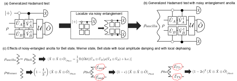
Figure S1: (a) Generalized Hadamard test, which includes non-local controlled operations.
(b) Generalized Hadamard test for DQC by replacing non-local controlled operations with (noisy) entangled ancilla and local controlled operations
(c) Effects on the expectation value, in (b), with a Bell state ancilla, a Werner state ancilla, a Bell state ancilla with local amplitude damping noise, and a Bell state ancilla with local noise.
Here, we introduce a generalized Hadamard test for distant subsystems and because the generalized Hadamard test is a building block for many quantum algorithms using virtual operations Endo et al. (2021); Sun et al. (2022); Endo et al. (2022); Tsubouchi et al. (2023), including ours in the main text.
Figure S1(a) shows the quantum circuit of a generalized Hadamard test, which requires non-local interaction between subsystems and the ancilla qubit, where is some input state, are some operators, is a CPTP map, and is some measurement operator.
This circuit simultaneously provides their expectation values as
(S1)
(S2)
Combining this with and measurement as well as post-processing these measurement data, we can implement various virtual operations at the expectation value level that cannot be realized by physical CPTP maps Endo et al. (2021).
We consider the generalized Hadamard test for DQC by replacing non-local controlled operations in Fig. S1(a) with a (noisy) entanglement ancilla, , and local controlled operations (Fig. 1(b)).
Below, we show that a Bell ancilla state provides the same expectation value as in Eq. (S1) and some kinds of noisy Bell states, such as a Werner state or a Bell state with local amplitude damping and dephasing ( noise), only reduce the expectation value with a constant factor.
In many virtual protocols including our protocol, this reduction does not affect the expectation value due to the division in the post-processing for normalizing the unphysical density matrix, as we see in Eq. (2) in the main text.
S1.1 Bell-diagonal state for the Bell state and a Werner state ancilla
Here we consider the Bell-diagonal state, defined as
(S3)
(S4)
where and
(S5)
Note that for and for .
The expectation value of the measurement on this state, in Fig. S1(b), is
(S6)
(S7)
(S8)
We can immediately see that the Bell state ancilla provides the same expectation value as in Eq. (S1) by setting ,
(S9)
By setting , we see that a Werner state ancilla, provides the expectation value as
(S10)
For the general Bell diagonal state, the bias term in Eq. (S8) vanishes when , and we obtain the desired expectation value with reduced amplitude by a factor of .
S1.2 A Bell state with a local amplitude damping noise
Here we consider the case where the ideal Bell state ancilla suffers from a local amplitude damping noise shown in Fig. S1(b), described as , where
(S11)
are Klaus maps.
Since the state is described as
(S12)
(S13)
the expectation value is calculated as
(S14)
Note that a similar calculation works for a global amplitude damping noise.
Therefore, when amplitude damping is dominant, we do not need twirling to make a Werner ancilla state.
S1.3 A Bell state with a local dephasing () noise
Then we consider the case where the ideal Bell ancilla state suffers from a local dephasing () noise described as .
Since the state is described as
(S15)
(S16)
the expectation value is calculated as
(S17)
Therefore, when a local dephasing () noise is dominant, we do not need twirling to make a Werner state.
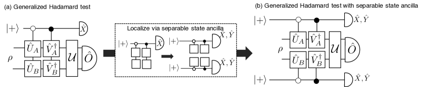
S2 Using separable ancilla state instead of noisy-entanglement ancilla state
Figure S2: (a) Generalized Hadamard test, which includes non-local controlled operations.
(b) Generalized Hadamard test for DQC by replacing non-local controlled operations with the separable state ancilla, and by implementing additional measurement.
In the main text, we replace the non-local controlled operation with noisy entanglement ancilla and local controlled operations.
Here, we show another replacement using separable state ancilla, and additional measurement as shown in Fig. S2.
As shown below, this replacement doubles the sampling-cost factor , leading to four-times sampling overhead.
Combining this replacement with the ancilla reuse in the main text provides asymptotically optimal circuit knitting as shown in Fig. 1 in the main text.
The calculation is similar to that for noisy entanglement above.
Since the separable state ancilla is described as
(S18)
the expectation values of and are calculated as
(S19)
(S20)
respectively.
From these expectation values, we have
(S21)
which is the same expectation value as that in Eqs. (S1) and (S9).
However, the additional measurement increases the variance of by a factor of four, leading to a sampling overhead of four times.
This means that the additional measurement doubles .
A simple explanation of this is as follows.
When we calculate by Monte-Carlo sampling, we may sample each term with a probability of , and thus we must multiply two to the sampling result, which increases its variance by a factor of four:
(S22)
For more general discussion, see Ref. Cai (2021b) for general observable.
S3 Effect of the noise in purification circuit
Figure S3: Quantum circuits sampled for our numerical demonstration to calculate the fidelity, where we set . Here, denotes the Bell measurement. The purification operation map including noise in LOCC is classified as , where is the identity map, is the map including only single-qubit gates, and the map including two-qubit gates.
The error maps, , describe local 1-qubit and 2-qubit noise map and measurement noise, respectively.
S3.1 Details in numerical calculation
In the numerical calculation for estimating the fidelity within local noise, we use quantum circuits shown in Fig. S3, where we set for calculating the fidelity and for simplicity.
Denoting the virtually purified state as , we obtain the purified fidelity to the Bell state as
(S23)
where is the purification operation map including noise, shown as in Fig. S3: when there is no noise in purification operations, and .
In the numerical calculation, we use only six quantum circuits including control operation (shown as in Fig. S3) instead of 12 quantum circuits because each circuit can sample two terms in at once.
For example, the quantum circuit at the top left within the dashed lines for generates , so we can obtain two terms at once when we sample this quantum circuit with the probability of .
S3.2 Analytical validation of the infidelity
We classify the purification operation as , where is the identity map, is the map including only single-qubit gates, and the map including two-qubit gates, because , , and affect differently on each map.
Here,
(S24)
is the measurement noise,
(S25)
is the single-qubit noise, and
(S26)
is the 2-qubit noise.
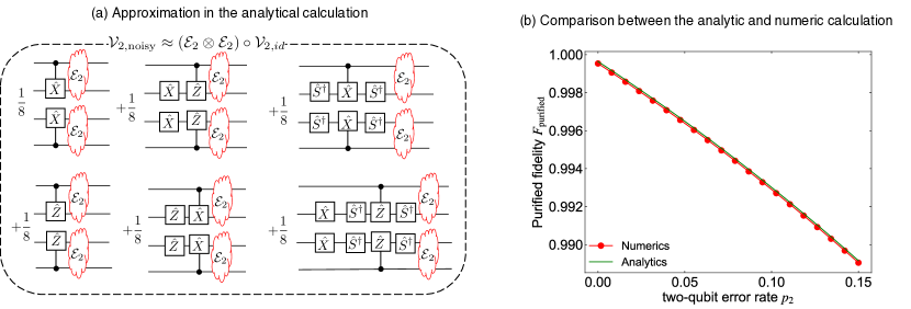
Here, we analytically show that the infidelity becomes with approximating for simplicity, where is the purification operation including two-qubit gates without noise in purification operations; see Fig. S4(a).
In the following, and are defined in the same way.
We show Fig. S4(b) in advance to convince the validity of these approximations to explain the behavior of dependence of the fidelity.
Figure S4: (a) Schematic quantum circuits of the approximation used in the analytical calculation. (b) 2-qubit error-rate dependence of purified fidelity for numerical and analytical results in Eq. (1) and Eq. (S43), respectively. The correspondence shows that the analytic calculation with the approximation explains the numerical result well.
To calculate the fidelity in the presence of noise in the purification operation, we would like to calculate
(S27)
for .
For preparation, we first examine the effects of single-qubit and 2-qubit noise and measurement noise in the expectation value.
Notably, as we show below, the 2-qubit noise and the measurement noise only reduce the amplitude of the expectation value, which is different from the effects on a state itself.
This is the essence of the low infidelity of our protocol.
First, for any operator and any state , the measurement noise and the two-qubit noise only reduce the amplitude of the trace by a factor of and , respectively, as follows.
For the measurement noise for any states , we have
(S28)
where we used
(S29)
This calculation shows that the measurement noise only reduces the amplitude of the expectation value.
For the two-qubit noise for any states , we have
(S30)
where we used
(S31)
(S32)
Here the terms in the second and third lines vanish because
(S33)
Finally, we consider the single-qubit noise.
For any state , we have
(S34)
(S35)
where we used
(S36)
(S37)
The purified fidelity in Eq. (S23) is calculated as
(S38)
(S39)
(S40)
where we used the approximation,, in the last line; see also Fig. S4(a) for this approximation.
By using , , and as a shorthand notation, and by using Eqs. (S28), (S30), and (S37), we continue the calculation as below:
(S41)
(S42)
(S43)
(S44)
Here, is the initial infidelity of the noisy Bell state.
Therefore, the infidelity after our protocol is .
We used the following calculations from the first to the second lines:
(S45)
(S46)
(S47)
(S48)
(S49)
(S50)
(S51)
(S52)
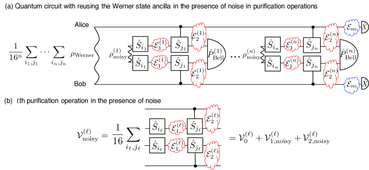
S4 Estimation of fidelity and for reusing the Werner state ancilla using data
Figure S5: (a) A quantum circuit to calculate the fidelity with ancilla reuse in the presence of noise. (b) The -th purification operation in the presence of noise.
Here we analytically calculate the fidelity and the sampling-cost factor for reusing a Werner ancilla state (Fig. S5 (a)), based on the data for with noisy purification operations.
As shown in Fig. S7 later, we confirm the correspondence between this estimation and the numerical calculation for .
To estimate the fidelity, yield, and , we need to calculate
(S53)
where
(S54)
is the noisy operations between the ancilla and -th noisy state, where is the identity map, is the map including only single-qubit gate, and is the map including two-qubit controlled gate as shown in Fig. S5: see also Fig. S3.
S4.1 Noiseless purification operations
Before considering noise in the purification operations, we review the calculation of the expectation value with the ancilla reuse without noise.
As in the previous section, we denote the purification map without noise as .
Denoting and is the -th operation on the ancilla state and without noise as shown in Fig. S5, we have
(S55)
(S56)
(S57)
where we defined .
We can obtain the expectation value as
(S58)
Note that setting gives the fidelity of noisy states to the ideal Bell state, which is unity without the presence of noise in the purification operations.
The sampling cost is proportional to the inverse of the denominator, as
(S59)
where is the fidelity for -th noisy state.
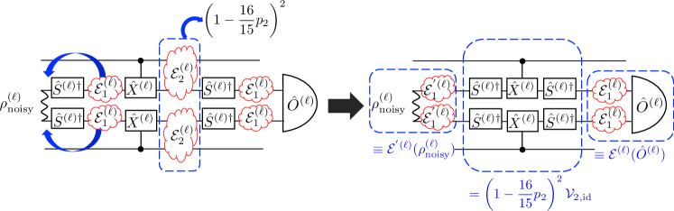
S4.2 Noisy LOCC
With noise in LOCC for the ancilla reuse, we need numerical calculation to obtain the fidelity, yield, and , although it is difficult for large due to its heavy numerical calculation.
Instead, we avoid this heavy numerical calculation by using data as follows.
Figure S6: Schematic illustration of the attribution of noise to the -th noisy state and -th measurement, taking one of the quantum circuits in as an example.
The essential point to proceed with the calculation is that the two-qubit noise in only reduces the amplitude of the trace as in Eq. (S30) as
(S60)
and thus the noise in in the trace can be considered to affect only on the -th noisy state and as , where and are single-qubit noise maps deformed by a single-qubit gate included in (see Fig. S6).
Then all the noise in attribute to the -th noisy state and the -th measurement , thereby decomposing the trace as follows.
(S61)
(S62)
(S63)
(S64)
Here, we define and as the single-qubit noise including the effect of and , respectively (see Fig. S6).
Figure S7: Analytical estimation and numerical data for (a) fidelity and (b) sampling-cost factor per purified states , .
In the numerical setting, we consider the same condition for all , that is,
can be obtained by the numerical simulation for .
This equation allows us to calculate the fidelity, yield, and for any by using only the data for .
Figure S7 shows this analytical estimation and numerical calculation for .
As we observe, this analytical estimation perfectly corresponds to the numerical calculation.
S5 Probabilistic error cancellation (PEC) for Bell-state preparation using only LOCC
PEC is one of the error mitigation methods Temme et al. (2017); Endo et al. (2018, 2021),
which effectively operates the inverse of the error map by post-processing at the cost of the number of sampling.
Suppose the ideal noiseless state is and the error map on the ideal state is .
By decomposing the inverse of the error map as with , the error-mitigated state is described as .
To simulate this decomposition with negative probability, we rewrite it as , where is the sampling-cost factor and is the sampling probability.
The number of sampling that needs to obtain the same accuracy without PEC scales with Endo et al. (2018).
Here we use PEC to suppress the error of a noisy Bell state.
We consider a protocol for a Werner state without loss of generality since any bipartite noisy state can be transformed by an appropriate twirling into a Werner state Bennett et al. (1996b).
Although Ref. Yuan et al. (2024) recently shows the inverse map that satisfies the lower bound of the sampling cost for PEC, we provide a practical and concrete protocol by constructing the inverse map using only Pauli operations and by providing the efficient estimation for the error rate.
Figure S8: Schematic illustration of probabilistic error cancellation (PEC) for a noisy Bell state .
In PEC, we insert with probability , with , with , and with , respectively, and then we multiply with the output of the last measurement.
S5.1 PEC for Bell-diagonal state
Here, we explain the application of PEC to the Bell-diagonal state defined as in Eq. (S3).
Any bipartite noisy state can be transformed by an appropriate twirling into a Bell-diagonal state Bennett et al. (1996b).
After twirling, we need to estimate the error rates, () for the Bell-diagonal (Werner) state.
This could be done by standard tomography methods.
Inspired by Ref. Piveteau et al. (2021), here we present a more efficient method described below, which uses a remote gate operation that has the property of for ; for example, we can use remote CNOT gates, which is .
We can estimate from the expected value obtained by preparing state, applying non-local remote gates with noisy Bell states times, , and measuring the output in the basis.
The expected value of the outcome as .
By doing the above procedure for different and using the exponential fitting, we can estimate .
Especially, since at is the fixed value, the simplest way is to do the above procedure for and use the exponential fitting for these two points.
Similarly, we can estimate by preparing state, applying non-local remote gates with noisy Bell states times, and measuring the output in the basis, whose expectation value of the outcome as .
Moreover, by preparing state, applying non-local remote gates with noisy Bell states times, and measuring the output in the basis, with which we can estimate the expectation value of the outcome as .
Note that, for a Werner state, we only have to do one estimation of the three kinds of estimation above since .
Once we estimate the error rate , we can apply the inverse map as follows:
(S73)
where
(S74)
(S75)
(S76)
(S77)
The sampling overhead is
(S78)
The derivation of these values is almost the same as the PEC for stochastic Pauli error, which is explained in, for example, App. A in Ref. Suzuki et al. (2022).
The whole protocol is as follows.
1.
Alice and Bob share the noisy Bell state. The noise information has to be obtained anyway to decide for .
2.
Alice samples with probability and tells to Bob. Similarly to the procedure of VQED, a person who samples can be Bob or another person.
3.
Alice and Bob apply the corresponding operation to the shared noisy Bell state, for , for , for , for , respectively.
4.
Run the whole quantum circuit, multiply to the outcome.
5.
Average the outcome to obtain the desired expectation value.
S5.2 PEC for a Werner state
For a Werner state, we require the error information for PEC, which is obtained by various tomography methods.
We here show the following method inspired by Ref. Piveteau et al. (2021), which uses a remote gate operation with a Werner state that has the property of for ; for example, we can use remote CNOT gates, which is .
We can estimate from the expectation value obtained by preparing state, applying non-local remote gates with noisy Bell states times, , and measuring the output in the basis.
The expectation value of the outcome is .
Doing the above procedure for different and using the exponential fitting estimates .
Especially, since at is the fixed value, the simplest way is to do the above procedure for and use the exponential fitting for these two points.
Once we estimate the error rate, we can apply the inverse map as
(S79)
where ,
.
The sampling overhead is
(S80)
The whole protocol for Alice and Bob is as follows.
1.
Alice and Bob share a noisy Bell state, twirls it into a Werner state and obtain its noise information anyway to decide for .
2.
They sample and share with probability .
3.
They apply the corresponding operation to the shared noisy Bell state, for , for , for , for , respectively.
4.
They run the whole quantum circuit, multiply to the outcome.
5.
They average the outcome to obtain the desired expectation value.