Exact Computation of Error in Approximate Circuits using SAT and Message-Passing Algorithms

Abstract

Effective usage of approximate circuits for various performance trade-offs requires accurate computation of error. Several average and worst case error metrics have been proposed in the literature. We propose a framework for exact computation of these error metrics, including the error rate (ER), mean absolute error (MAE), mean squared error (MSE) and the worst-case error (WCE). We use a combination of SAT and message-passing algorithms. Our algorithm takes as input the CNF formula for the exact and approximate circuits followed by a subtractor that finds the difference of the two outputs. This is converted into a tree, with each vertex of the tree associated with a sub-formulas and all satisfying solutions to it. Once this is done, any probability can be computed by setting appropriate error bits and using a message passing algorithm on the tree. Since message-passing is fast, besides ER and MAE, computation of metrics like MSE is also very efficient. In fact, it is possible to get the entire probability distribution of the error. Besides standard benchmarks, we could compute the error metrics exactly for approximate Gaussian and Sobel filters, which has not been done previously.

I Introduction

Over the past decade, approximate circuits have gained traction as an effective method to trade off error for performance metrics like energy savings and frequency of operation in error tolerant applications. Computing the error in these circuits is an essential step towards determining the acceptability of the approximation. The system (S) used for error analysis consists of the exact and approximate circuits along with an error miter that models the desired error metric. In this paper, our focus is on exact computation of average and worst case error metrics that have been proposed in the literature. This includes the error rate (ER), mean absolute error (MAE), mean squared error (MSE) and the worst case error (WCE). Evaluation of these error metrics exactly is challenging since the outputs of both the exact and approximate circuits have to be known for all possible values of the inputs.

In the past, methods used for exact error analysis include exhaustive enumeration, analysis based on binary and algebraic decision diagrams (BDD/ADD) and model counting (#SAT) based analysis. Exhaustive enumeration is infeasible for larger circuits. BDD based error analysis techniques have been proposed in [1, 2, 3, 4, 5]. In these methods, a BDD is constructed for the entire system S and traversal of the BDD is used to compute the error metrics. The miters used for various error metrics are included in [3]. An alternate method based on symbolic computer algebra and construction and traversal of ADDs has been proposed in [6, 7]. The advantage of their technique is that a single method can be used to get all error metrics, including relative errors.

Methods proposed in [8, 9] use model counting for computation of certain error metrics. WCE analysis in particular can be performed effectively using SAT solvers [8, 3]. In [9], the authors propose circuit aware model counter VACSEM that integrates logic simulation into a #SAT solver GANAK [10] and use it to compute ER and MAE.

I-A Motivation

BDD based methods have shown limited scalability and we have not seen results for metrics like MAE and MSE for beyond 32-bit approximate adders. The #SAT solver VACSEM has proved to be efficient for computation of ER and MAE of up to 128-bit adders and 16-bit multipliers. Their method depends on partitioning the system into single output sub-miters. It does not allow for a straightforward extension to computing metrics that require a sat-count for a joint assignment of the error bits, as for example MSE. Moreover, each new error metric in VACSEM requires construction of the corresponding error miter, partitioning of the system based on the output of the error miter and re-synthesizing the partitions before model counting. In this respect, the one-method-fits-all proposed in [7] is attractive, but has shown limited scalability.

I-B Contribution

Our algorithm takes as input the CNF formula for the exact and approximate circuits followed by a subtractor that finds the difference of the two outputs. This is converted into a tree, with each vertex of the tree associated with a sub-formulas and all satisfying solutions to it. Once this is done, any probability can be computed by setting appropriate error bits and using a message passing algorithm on the tree. Since message-passing is fast, besides ER and MAE, computation of metrics like MSE is also very efficient. In fact, it is possible to get the entire probability distribution of the error. Besides standard benchmarks, we are able to compute metrics for 128 bit adders as well as approximate Gaussian and Sobel filters, with competitive runtimes.

II Background and Notation

II-A Notation

Our system consists of the exact and approximate circuits and a subtractor that computes the difference of the two outputs. Let $y,\hat{y}\colon\mathbb{B}^{n}\to\mathbb{B}^{m}$ denote the outputs of the exact and approximate circuits. $E=y-\hat{y}$ is the $m+1$ bit error, obtained as the output of the subtractor in the twos complement form. We denote the ith bit of $y,\hat{y}$ and $E$ as $y_{i},\hat{y}_{i}$ and $e_{i}$, respectively. Let $\mathbf{F}$ denote the formula for the system in the CNF form. Model counting or #SAT computes the total number of satisfying solutions for $\mathbf{F}$, which we denote $\mathit{sat-count(\mathbf{F})}$. $\mathit{sat-count}$($e_{i}$) denotes $\mathit{sat-count}$$(\mathbf{F}\mid e_{i}=1)$.

II-B Error metrics

A detailed discussion of the error miters for commonly used error metrics can be found in [3]. For convenience, we briefly discuss the miters for ER, MAE, MSE and WCE.
Error Rate:(ER) It is the probability of getting an erroneous output. The miter generally used [3] consists of $m$ XOR gates with inputs $y_{i}$ and $\hat{y}_{i}$ followed by a tree of OR gates.
Mean absolute error:(MAE) It can be derived as [3]

$$\mathrm{MAE}(y,\hat{y}) =\frac{1}{2^{n}}\left(\mathit{sat-count}(e_{m})+\sum_{i=0}^{m-1}2^{i}\mathit{sat-count}(e_{i}\oplus e_{m})\right)$$ (1)

Mean Squared error:(MSE) It can be computed as

$$\mathrm{MSE}(y,\hat{y})=\frac{1}{2^{n}}\left(\sum_{i=0}^{m}2^{2i}\mathit{sat-count}(e_{i})~{}+\right.$$ (2)

$$\left.\sum_{i=0}^{m-1}\sum_{j=i+1}^{m-1}2^{i+j+1}\mathit{sat-count}(e_{i}\land e_{j})-\sum_{i=0}^{m-1}2^{i+m}\mathit{sat-count}(e_{i}\land e_{k})\right)$$

Worst case error:(WCE) It can be either positive ($e_{m}=0$) or negative ($e_{m}=1$). To find positive WCE, each bit from $m-1$ to $0$ is tested for SAT with all prior satisfied bits added as unit clauses to $\mathbf{F}\land\neg e_{m}$. The positive WCE is the binary number with all the SAT bits set to one and rest to zero. For negative WCE, the same procedure is followed with SAT for complement of the error bits and $\mathbf{F}\land e_{m}$. One is added in the end to the negative WCE to get the two’s complement. The overall WCE is the maximum of the magnitudes of positive and negative ones.

II-C Factor and Factor product

A factor $\phi(\mathbf{Y})$ is a function that maps all possible assignments of variables in $\mathbf{Y}$ (denoted Domain($\mathbf{Y}$)) to a non-negative real number, that is $\phi(\mathbf{Y})$ : Domain$(\mathbf{Y})\to\mathbb{R}\geq 0$. At several points in our method, we need to compute a factor product defined as follows. Let $\mathbf{X},\mathbf{Y},\mathbf{Z}$ be disjoint sets of variables and $\phi_{1}(\mathbf{X},\mathbf{Y}),\phi_{2}(\mathbf{Y,Z})$ be two factors. The factor product [11, Chapter 4] $\phi_{1}\phi_{2}$ gives a factor $\psi$ which is obtained as follows.

$$\forall x,y,z\in\textrm{Domain}(\mathbf{X,Y,Z}),$$

$$\psi(\mathbf{X},\mathbf{Y},\mathbf{Z}=x,y,z)=\phi_{1}(x,y)\phi_{2}(y,z)$$

II-D Message passing

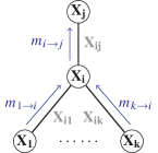
Figure 1: Message passing for a tree. The messages are passed from leaves to the root.

The sum-product algorithm, which is used to find the marginal probabilities and partition function of Markov networks, can be implemented using a message passing (MP) algorithm on a graphical representation of the network [11]. The product refers to a factor product. MP works as follows. Each node of a tree is associated with a set of variables $\mathbf{X_{i}}$ and a factor $\psi_{i}(\mathbf{X_{i}})$. Let $\mathbf{X_{ij}}$ denote the variables common to nodes $\mathbf{X_{i}}$ and $\mathbf{X_{j}}$. The message $m_{i\rightarrow j}$ from node $i$ to node $j$ is computed using the following sum-product operation.

$$m_{i\rightarrow j}(\mathbf{X_{ij}})=\sum\limits_{\mathbf{X_{i}}\setminus\mathbf{X_{ij}}}\psi_{i}\prod_{k\in\text{Neighbours}(i)\setminus j}m_{k\rightarrow i}(\mathbf{X_{ik}})$$ (3)

Essentially, the factor product of $\psi_{i}$ and incoming messages from the neighbours of $i$ other than $j$ is marginalized over variables that are not shared by nodes $i$ and $j$.

III Proposed Algorithm

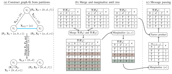
Figure 2: (a) Partitioning the CNF formula $\mathbf{F}$ with error variables $e$ and $f$ into $\mathbf{F_{1},F_{2},F_{3}}$ and constructing graph $\mathbf{G}$ (b) Merging $\mathbf{F_{1}}$ and $\mathbf{F_{2}}$ and marginalizing $\mathbf{X_{1,2}}$ w.r.t $\{a,c\}$ (c) Message passing

Let $\mathbf{X}$ be the set of variables in the formula $\mathbf{F}$, $\mathbf{S(F)}$ be the set containing all satisfying solutions of $\mathbf{F}$. Our algorithm has the following steps.

III-1 Partition and model count for partitions

We first convert $\mathbf{F}$ into a hypergraph using the method in [12]. Each clause in $\mathbf{F}$ is a vertex in the hypergraph and each variable $x\in\mathbf{X}$ is a hyperedge. A hyperedge $x$, connects all the vertices(clauses) that contain $x$ or its complement. A hypergraph partitioner is then used to partition $\mathbf{F}$ into $P$ partitions, $\mathbf{F}_{1},\cdots,\mathbf{F}_{P}$, such that $\mathbf{F}=\bigwedge_{i=1}^{P}\mathbf{F}_{i}$ and $\mathbf{X}=\bigcup_{i=1}^{P}\mathbf{X}_{i}$. The partitioning is done with a limit on the maximum number of clauses in each partition. To partition the hypergraph corresponding to $\mathbf{F}$, we use the hypergraph partitioner [13]. It produces partitions with minimum number of cuts, which corresponds to minimizing the number of shared variables between partitions.

Following this, we use a #SAT solver to obtain $\mathbf{S(F_{i})}$. This is efficient since the number of clauses in each partition is limited. For each partition, we construct a table $\mathbf{T(F_{i})}=\{s\in\mathbf{S(F_{i})},c(s)\}$, where $c(s)$ is the number of solutions containing the assignment $s$. At this point $c(s)=1$ for all entries in the table and $\mathit{sat-count}(\mathbf{F_{i}})=\sum_{s}c(s)$. Note that each table is a factor. Fig. 2(b) shows an example CNF $\mathbf{F}$ partitioned into three partitions, $\{\mathbf{F_{1},F_{2},F_{3}}\}$ and their corresponding tables $\mathbf{T(F_{i})}$.

III-2 Graph construction

The partitioned formula is converted to graph $G$ as follows. The vertices of $G$ are $V_{i}=\{\mathbf{F_{i}},\mathbf{X_{i}},\mathbf{T(F_{i})}\}$. Each table is a factor associated with the corresponding vertex. An edge $E_{i,j}$ connects two vertices $V_{i}$ and $V_{j}$ in $G$ if $\mathbf{X_{i}}\cap\mathbf{X_{j}}\neq\emptyset$. Fig. 2(a) shows the example graph G with $\mathbf{X_{i,j}}$ shown on the edges.

III-3 Merge and Marginalize

Assume that $V_{i}$ and $V_{j}$ are connected by an edge $E_{i,j}$. $\textnormal{Merge}({G},V_{i},V_{j})$ replaces the two vertices by a single vertex $V_{i}$ associated with the formula $\mathbf{F_{i}}\land\mathbf{F_{j}}$ and the modified variable set $\mathbf{X_{i}}=\mathbf{X_{i}}\cup\mathbf{X_{j}}$. The resultant table $\mathbf{T}(\mathbf{F_{i}})$ is the factor product of $\mathbf{T(F_{i})}$ and $\mathbf{T(F_{j})}$. It contains all satisfying solutions ${s}$ of the modified formula with $c(s)=c(s_{i})\times c(s_{j})$. The total number of satisfying solutions of the merged node is $\mathit{sat-count}(\mathbf{F_{i}})=\sum_{s}c(s)$. Neighbours of ${V_{j}}$ are then connected to ${V_{i}}$, with the same associated common variables. For any ${V_{k}\in\text{Neighbour}({V_{j}})}$ if $\mathbf{X_{k}}\subset\mathbf{X_{i}}$, then ${V_{k}}$ is also merged with ${V_{i}}$. This merge will not result in any increase in the table size, but the counts in $\mathbf{T(F_{i})}$ will get updated. Fig. 2(b) shows an example where the tables $\mathbf{T(F_{1})}$ and $\mathbf{T(F_{2})}$ are merged resulting in an updated $\mathbf{T(F_{1})}$.

Marginalize: Let $Q_{i}=\{x:x\notin E~{}\textrm{and}~{}x\in\mathbf{X_{i}},x\notin\mathbf{X_{j}},j\neq i\}$ be the set of variables that are not the error variables and are present exclusively in $\mathbf{X_{i}}$. The marginalization step removes the variables $x\in Q_{i}$ from $\mathbf{T(F_{i})}$ and updates the table as follows. For each $x$, if $s_{0}=\{s,x=\mathrm{False}\}$ and $s_{1}=\{s,x=\mathrm{True}\}$ are satisfying assignments of variables for $\mathbf{F_{i}}$, then

$$\mathbf{T(F_{i})}=\{s\in\mathbf{S(F_{i})},c(s)=c(s_{0})+c(s_{1})\}$$

The variable list in $\mathbf{F_{i}}$ is updated as $\mathbf{X_{i}}=\mathbf{X_{i}}\setminus Q_{i}$. Fig. 2(b) illustrates the marginalization of $Q_{1}=\{a,c\}$ from $\mathbf{T(F_{1})}$.

Algorithm 1 has the main steps. The vertices that result in smaller table sizes are preferred for merging. An estimate of the size of the merged table is used to choose the vertex pairs. The edges are sorted in increasing order of the estimated merged sizes. Edges with estimates larger than a predefined limit are filtered. Pairs of vertices from disjoint edges in this filtered list are chosen greedily to merge starting with the least size. The Merge and Marginalize steps procedure continues until the graph G becomes a tree or the nodes can no longer be merged without the resultant table size exceeding the limit.

Algorithm 1 Merge and Marginalize until tree

0:  CNF $\mathbf{F}$, Number of partitions $p$, Table size threshold $TS$

1:  $\{\mathbf{F_{1},F_{2},\dots F_{p}}\}\mathrel{\hskip 1.0pt=\hskip 1.0pt}\textnormal{Partition}(\mathbf{F},p)$

2:  Construct an undirected-graph $G=(V,E)$ with$V_{i}=\{\mathbf{F_{i}},\mathbf{X_{i}},\mathbf{T(F_{i})}\}$, $E=(\{V_{i},V_{j})\mid V_{i},V_{j}\in V,\mathbf{X_{i,j}}\neq\emptyset\}$

3:  while $G$ is not a tree do

4:     for all $(V_{i},V_{j})\in E$ do

5:        $w_{i,j}$ = Estimated size of merging $\mathbf{T(F_{i})}$ and $\mathbf{T(F_{j})}$

6:     end for

7:     Sort $E$ in increasing order of $w_{i,j}$

8:     L $\mathrel{\hskip 1.0pt=\hskip 1.0pt}$ Filter edges in $E$ with $w_{i,j}>TS$ and choose disconnected edges with smallest weights

9:     for all $(V_{i},V_{j})\in L$ do

10:        $V_{i}\mathrel{\hskip 1.0pt=\hskip 1.0pt}\{\mathbf{F_{i}}\land\mathbf{F_{j}},\mathbf{X_{i}}\cup\mathbf{X_{j}}$, FactorProd$(\mathbf{T(F_{i})},\mathbf{T(F_{j})})$}

11:     end for

12:     Rebuild $G$ with updated $V_{i}$

13:     for all $V_{i}\in V$ do

14:        $\mathbf{X_{\text{marg}}}\mathrel{\hskip 1.0pt=\hskip 1.0pt}\mathbf{X_{i}}\setminus\bigcup\limits_{(V_{i},V_{j})\in E}\mathbf{X_{j}}$ // variables unique to $\mathbf{X_{i}}$

15:        Marginalize($\mathbf{T(F_{i})}$, $\mathbf{X_{\text{marg}}}$)

16:     end for

17:  end while

The tables used in our merge algorithm are hash tables with (satisfying solutions, counts) forming the (key, value) pairs. The satisfying solutions are stored as compact bit-vectors to minimize the table’s memory footprint. A efficient parallel hash table [14] is used in our implementation. To decide if two connected vertices can be merged, an estimate of the resultant table size after merging is required. An exact estimate involves counting the distinct assignments in the merged table which is runtime/memory intensive. An approximate estimate is adequate for relative ordering of edges and filter edges with large tables. This is the standard count-distinct problem in data streams, efficiently solved by the HyperLogLog algorithm [15].

III-4 Message passing

We use the message passing algorithm on the tree obtained after the Merge and marginalize procedure in order to get the desired $\mathit{sat-count}$. Use of the message-passing algorithm requires that the tree satisfies the running intersection property (RIP). This property is defined as follows: if vertices $V_{i}$ and $V_{k}$ share a variable $x$, then every vertex $V_{j}$ in the path between $V_{i}$ and $V_{k}$ must contain $x$. The tree obtained after the Merge and Marginalize algorithm always satisfies this property, as shown in the following theorem.

Theorem 1.

When graph $G$ becomes a tree, (RIP) is satisfied.

Proof.

The initial graph G is constructed so that there is an edge between a pair of vertices in G iff they have variables in common. When the Merge step merges $V_{j}$ with $V_{i}$, neighbours of ${V_{j}}$ are connected to ${V_{i}}$ with each edge associated with the same common variables. Marginalization does not affect variables associated with the edges. After repeated merge-and-marginalize steps, assume that G is converted to a tree. The proof is by contradiction. Assume RIP is not satisfied. This implies there exists ${V_{j}}$ in the path from $V_{i}$ to $V_{k}$ with $x\in\mathbf{X_{i}}$ and $x\in\mathbf{X_{k}}$, but $x\notin\mathbf{X_{j}}$. By definition, there must be an edge from ${V_{i}}$ to ${V_{k}}$ resulting in a loop, which is not possible since G is a tree. ∎

The message passing algorithm is implemented as follows. The graph G is now considered as a rooted directed tree, with tables $\mathbf{T(F_{i})}$ associated with vertex $V_{i}$. Each table is modified using messages from its children as follows

$$\mathbf{T(F_{i})}\mathrel{\hskip 1.0pt=\hskip 1.0pt}\mathbf{T(F_{i})}\cdot\prod_{v\in\mathrm{children}(i)}m_{j\to i}$$ (4)

A node in the tree can be updated only after all its children are updated. The product in equation (4) is a factor product. The message $m_{j\rightarrow i}$ from node $j$ to node $i$ is a factor (table) that is computed as follows. The variables in the table are the common variables $\mathbf{X_{i,j}}$. Let $s$ denote an assignment of $\mathbf{X_{j}}$ and $s_{x}$ an assignment of $\mathbf{X_{i,j}}$ To get the number of satisfying solutions $c(s_{x})$, we marginalize over the variables $\mathbf{X_{j}}\setminus\mathbf{X_{i,j}}$, i.e.,

$$c(s_{x})=\sum_{\mathbf{{X_{j}}}\setminus\mathbf{X_{i,j}}}c(s)$$ (5)

Therefore, $m_{j\rightarrow i}=\{s_{x},c(s_{x})\}$. This is illustrated in Fig.2(c) for the example. As shown in the figure, after the Merge and marginalize procedure, we have two tables $\mathbf{T(F_{1}})$ and $\mathbf{T(F_{3})}$. The variables common to the two tables are $b$ and $d$. The message $m_{1\rightarrow 3}$ is the table obtained after marginalizing the variable $e$.

Algorithm 2 has the main steps in the message passing algorithm. It first picks the root node $r$ and adds all the leaf nodes to a queue. A node is popped from the queue, a message is passed from the node to its parent and the corresponding factor product is computed. Once the node has received messages from all its children, it is added to the queue. The procedure terminates once we reach the root node, at which point the queue is empty.

The required $\mathit{sat-count}$ can be computed using the following theorem

Theorem 2.

On termination of the MP algorithm, the required $\mathit{sat-count}$ for $\mathbf{F}$ can be obtained as

$$\mathit{sat-count}(\mathbf{F})=\sum_{s\in\mathbf{T}(\mathbf{X_{r}})}c(s)$$

where $r$ is the root node and $\mathbf{T}(\mathbf{X_{r}})$ is the table corresponding to the root node.

Proof.

Assume that the tree consists of two nodes $V_{1}$ and $V_{2}$ with variables $\mathbf{X_{1}}$ and $\mathbf{X_{2}}$, representing the formula $\mathbf{F}=\mathbf{F_{1}}\wedge\mathbf{F_{2}}$. Let the tables for the two nodes be $\mathbf{T}(\mathbf{X_{1}})=\{s,c(s)\}$ and $\mathbf{T}(\mathbf{X_{2}})=\{\tilde{s},c(\tilde{s})\}$, where $s$ and $\tilde{s}$ are satisfying assignments of $\mathbf{F_{1}}$ and $\mathbf{F_{2}}$. Let $\mathbf{X_{12}}=\mathbf{X_{2}}\cap\mathbf{X_{2}}$. Then $m_{j\to i}=\mathbf{T}(\mathbf{X_{12}})=\{s_{12},\hat{c}(s_{12})\}$, where $\hat{c}(s_{12})$ is obtained by marginalizing entries of $\mathbf{T}(\mathbf{X_{2}})$ over the $\mathbf{X_{2}}\setminus\mathbf{X_{12}}$ as shown in equation (5). The factor product $\mathbf{T}(\mathbf{X_{1}})m_{2\to 1}$ modifies $c(s)$ in $\mathbf{T}(\mathbf{X_{1}})$ as follows. For $s=\{s_{\mathbf{X_{1}}\setminus\mathbf{X_{12}}},s_{12}\}\in\mathbf{T}(\mathbf{X_{1}})$, $c(s)=c(s)\times\hat{c}(s_{12})$ i.e. it multiplies the count of the consistent solutions in the two tables. Therefore,

$$\sum_{s\in\mathbf{T}(\mathbf{X_{1}})}c(s)=\mathit{sat-count}(\mathbf{F})$$

In the MP algorithm, each node accumulates messages from its children and computes the factor product with its own table. The sum of the counts in the resulting table is thus the $\mathit{sat-count}$ for the conjunction of formulas of the node and its children. The theorem follows since the MP algorithm terminates when the root node receives messages from all its children. ∎

Fig. 2(c) depicts the message passing and factor product for finding the $\mathit{sat-count}$($\mathbf{F}$). $V_{3}$ is designated the root node and the factor product of $\mathbf{T}(\mathbf{X_{3}})$ and the message gives final table at the root, with $\mathit{sat-count}$($\mathbf{F})=8$.

Algorithm 2 Message passing on a tree and evaluation of $\mathit{sat-count}$

0:  Directed rooted tree $G\mathrel{\hskip 1.0pt=\hskip 1.0pt}(V,E)$

1:  $\mathit{r}$ $\mathrel{\hskip 1.0pt=\hskip 1.0pt}$ Root vertex of $G$

2:  $Q$ $\mathrel{\hskip 1.0pt=\hskip 1.0pt}$ {all leaves of $G$} // Initialize queue with leaves

3:  $D$ $\mathrel{\hskip 1.0pt=\hskip 1.0pt}$ $\emptyset$ // Processed vertices

4:  while $Q\neq\emptyset$ do

5:     for all $v\in Q$ do

6:        $u\mathrel{\hskip 1.0pt=\hskip 1.0pt}$ parent($v$)

7:        $\mathbf{T}(\mathbf{F}_{u})\mathrel{\hskip 1.0pt=\hskip 1.0pt}\mathbf{T}(\mathbf{F}_{u})\cdot m_{u\to v}$ // factor-product

8:     end for

9:     $D\mathrel{\hskip 1.0pt=\hskip 1.0pt}D\cup Q$// Messages passed for all $Q$

10:     $Q\mathrel{\hskip 1.0pt=\hskip 1.0pt}\emptyset$

11:     for all $v\in V$ do

12:        if $v\notin D$ and children($v$)$\in D$ then

13:           $Q\mathrel{\hskip 1.0pt=\hskip 1.0pt}Q\cup\{v\}$

14:        end if

15:     end for

16:  end while

17:  return  $\sum\limits_{s\in\mathbf{S}(r)}c(s)$ // sum the counts of the root

Source	Benchmark	Our approach runtime(s)								VACSEM runtime(s)
		Overhead		WCE	P(WCE)	ER	MSE	MAE	Total	ER	MAE
		P	I+M
BACS	abs_diff	0.06	0.02	0.0001	0.0001	0.0001	0.0001	0.0001	0.08	0.001	0.005
	adder32	0.001	0.48	0.0002	0.0001	0.0001	0.0005	0.0003	0.49	0.006	0.007
	buttfly	1.63	0.11	0.0031	0.0001	0.0001	0.0023	0.0005	1.76	0.012	0.354
	mac	0.0002	0.02	0.0002	0.0001	0.0001	0.0001	0.0001	0.02	0.001	0.003
	mult8	1.23	0.43	1.6363	0.0013	0.0013	0.0802	0.0371	3.41	0.002	0.003
	x2	0.19	0.03	0.0005	0.0006	0.0006	0.0168	0.0080	0.25	–	–
GeAr	ACA_II_N32_Q16	0.82	0.02	0.0020	0.0001	0.0001	0.0036	0.0004	0.86	–	–
	ACA_I_N32_Q8	1.74	0.25	0.0060	0.0022	0.0025	0.9958	0.0950	3.11	–	–
VACSEM	add128	2.77	0.25	0.0016	0.0001	0.0001	0.0003	0.0001	3.02	2.353	0.343
	binsqrd	1.58	0.77	0.0047	0.0074	0.0068	0.0462	0.0412	2.45	0.008	0.103
	mult10	1.58	6.35	0.0067	0.0091	0.0095	0.0774	0.0416	8.07	0.012	0.019

TABLE I: Runtimes to evaluate the error metrics for BACS and VACSEM benchmarks. P is the partitioner runtime and I+M is the runtime to initialize tables and recursively merge/marginalize.

III-5 Error-metric computation

In order to compute various metrics, we need to find the $\mathit{sat-count}$ for various assignments of the error bits. At this point the graph is a tree. Therefore, we just need to set the values of the error bits and run the message passing algorithm to get the required $\mathit{sat-count}$s. We compute ER as one minus the probability that the error is zero, which can be obtained by setting all the error bits to zero and finding the resultant $\mathit{sat-count}$. MAE and MSE are computed by running the MP algorithm for each setting of appropriate pairs of bits as shown in equations (1) and (2).

IV Results

All experiments were done on a Intel i7-13700 CPU with 64GB of RAM, running Ubuntu 24.04. In all our experiments, a maximum of eight threads were used to execute parallel portions of the code. The benchmarks used for the evaluation of our algorithms are: (a) BACS [16] benchmarks, (b) VACSEM [9], (c) Generic Accuracy (GeAr) configurable adders from KIT [17], (d) Low Power Approximate Adders (LPAA), including AMA [18], AXA [19], and LOA [20] of various lengths and (e) Gaussian-$3\times 3$ filter and Sobel filters.

Table I has the runtimes for various error metrics for select benchmarks from BACS, GeAr, and VACSEM. To compute any error metric using our algorithm, there is an overhead comprising CNF partitioning, initial table generation using #SAT solver [21], and merging and marginalizing. All error metrics are obtained after setting appropriate error bits and running the message passing algorithm. In these benchmarks, the majority of runtime is spent in the overhead part. It can be seen from the table that message passing takes an insignificant amount of the total time. Time taken for MSE is only marginally larger than MAE. The MAE and ER obtained matches with values obtained using VACSEM. For some of the smaller benchmarks we verified the other metrics with exhaustive enumeration. For ER and MAE, VACSEM is faster as seen in Table I. Note however, that the runtimes for VACSEM do not include the overhead of synthesizing multiple partitions. Not having to synthesize the netlist repeatedly for various error metrics is a salient attribute of our algorithm. Once the merge and marginalize routine generates a tree, message passing helps quickly evaluate all error metrics.

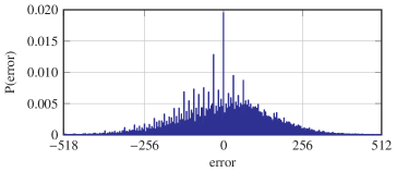
Figure 3: Histogram of error probabilities for the BACS benchmark mult8 generated using our algorithm.

One of the strengths of our algorithm is that we can obtain any probability, including the entire probability distribution of the error. Fig. 3 shows the histogram of error probabilities for the mult8 benchmark. It was obtained by setting the error bits for each possible value of the error and finding the resultant $\mathit{sat-count}$ using the message passing algorithm. Further, each data point on the histogram can be generated independent of others which helps in parallelization of the routine. For the mult8 benchmark, generation of histogram took 0.8s.

In Table II, we report the runtimes to compute the error metrics for three 128-bit low power approximate adders. The number of non-zero error bits in the output affects the runtime of all the steps in our algorithm. The graph $G$ used to merge and marginalize becomes proportionally denser. The tables are also larger since there are a larger number of variables that cannot be marginalized. The net effect of all these is the increase in runtimes. The column NE in Table II shows the number of error bits in the output of the adders. As expected, the runtimes increase with the number of approximate bits. We have tried up to 120 approximate bits, which is larger than the number of error bits in the approximate adders used to evaluate VACSEM (11 bits). The runtimes are also weakly dependent on the approximation used in the adder. The MSE for the approximate adders is larger than $10^{71}$ for 120 approximate bits. We could verify the MSE for some adders against analytical expressions [22]. This showcases the ability of our approach to compute such large errors accurately.

LPAA	NE	Runtime(s)
		Overhead		WCE	ER	MSE	MAE	Total
		P	I+M
AMA1	32	3.5	0.3	0.0247	0.0007	0.49	0.04	4.4
	64	3.7	0.4	0.0143	0.0010	1.31	0.05	5.5
	90	4.0	0.4	0.0153	0.0012	3.68	0.13	8.1
	120	4.2	0.4	0.0119	0.0007	8.37	0.15	13.1
AMA2	32	2.8	0.1	0.0075	0.0004	0.07	0.01	3.1
	64	2.7	0.1	0.0077	0.0003	0.22	0.01	3.1
	90	2.7	0.1	0.0080	0.0004	0.46	0.02	3.3
	120	2.6	0.2	0.0087	0.0003	1.24	0.03	4.1
AXA2	32	6.3	0.7	0.0195	0.0002	0.18	0.01	7.3
	64	5.8	0.7	0.0212	0.0003	0.70	0.07	7.4
	90	5.9	0.6	0.0214	0.0002	1.31	0.04	7.9
	120	5.6	0.9	0.0207	0.0011	12.36	0.69	19.6

TABLE II: Runtimes to evaluate the error metrics for various 128-bit LPAA adders. NE is the number of erroneous output bits; P is the partitioner runtime and I+M is the runtime to initialize tables and recursively merge/marginalize.

Table III has the results for $3\times 3$ approximate Gaussian and Sobel filters used in gradient filters for image processing. These have been recently used for design space exploration in [23]. The metric usually used is PSNR, which can be computed using MSE. Exact MSE for these filters has not been obtained previously. Only LOA has been used in [23], but we tried it with various approximate adders. The runtimes are less than 10s, showing that our tool is useful for exploration.

	LPAA	Runtime(s)
		Overhead		WCE	ER	MSE	MAE	Total
		P	I+M
G	AMA2	1.3	1.8	0.0598	0.0001	0.0016	0.0009	3.3
	AMA5	1.2	1.4	0.2613	0.0168	0.1840	0.0553	3.2
	AXA2	1.3	2.0	0.0749	0.0010	0.0138	0.0072	3.4
	LOA	1.6	1.5	0.1770	0.0424	0.8173	0.3294	4.6
S	AMA2	0.9	3.4	0.0006	0.0095	0.3645	0.1042	4.8
	AMA5	1.2	2.5	0.0005	0.0001	0.0045	0.0015	3.8
	AXA2	1.0	4.9	0.0005	0.0094	0.3526	0.0992	6.3
	LOA	1.0	0.9	0.0006	0.0001	0.0023	0.0008	2.0

TABLE III: Runtimes to evaluate the error metrics for filters; G and S are the 3x3 Gaussian and Sobel filters respectively. NE is the number of erroneous output bits; P is the partitioner runtime and I+M is the runtime to initialize tables and recursively merge/marginalize.

V Conclusion

We have proposed an algorithm based on #SAT and message passing that can be used for exact computation of a variety of error metrics. Besides the standard metrics, we can obtain various probabilities including the entire probability distribution function. We have been able to obtain MSE of approximate filters used in image processing, which has not been done previously.

Currently, we partition the problem by partitioning the hypergraph corresponding to the formula $\mathbf{F}$. In future, we plan to explore partitioning at the circuit level and then convert each partition into a CNF formula. Also, within our framework, we can also use BDDs, logic simulation or other methods to generate the initial tables.

References

- [1] M. Soeken, D. Große, A. Chandrasekharan, and R. Drechsler, “BDD minimization for approximate computing,” in Asia and South Pacific Design Automation Conference (ASP-DAC), pp. 474–479, 2016.
- [2] C. Yu and M. Ciesielski, “Analyzing Imprecise Adders Using BDDs – A Case Study,” in IEEE Computer Society Annual Symposium on VLSI (ISVLSI), pp. 152–157, 2016.
- [3] Z. Vasicek, “Formal Methods for Exact Analysis of Approximate Circuits,” IEEE Access, vol. PP, pp. 1–1, 12 2019.
- [4] Y. Wu and W. Qian, “ALFANS: Multilevel Approximate Logic Synthesis Framework by Approximate Node Simplification,” IEEE Trans. Comput.-Aided Design Integr. Circuits Syst., vol. 39, no. 7, pp. 1470–1483, 2020.
- [5] V. Mrazek, “Optimization of BDD-based Approximation Error Metrics Calculations,” in IEEE Computer Society Annual Symposium on VLSI (ISVLSI), pp. 86–91, 2022.
- [6] S. Froehlich, D. Große, and R. Drechsler, “Approximate hardware generation using symbolic computer algebra employing grobner basis,” in Design, Automation & Test in Europe Conference & Exhibition (DATE), pp. 889–892, 2018.
- [7] S. Froehlich, D. Große, and R. Drechsler, “One Method - All Error-Metrics: A Three-Stage Approach for Error-Metric Evaluation in Approximate Computing,” in Design, Automation & Test in Europe Conference & Exhibition (DATE), pp. 284–287, 2019.
- [8] M. Češka, J. Matyaš, V. Mrazek, L. Sekanina, Z. Vasicek, and T. Vojnar, “Approximating complex arithmetic circuits with formal error guarantees: 32-bit multipliers accomplished,” in IEEE/ACM International Conference on Computer-Aided Design (ICCAD), pp. 416–423, 2017.
- [9] C. Meng, H. Wang, Y. Mai, W. Qian, and G. De Micheli, “VACSEM: Verifying Average Errors in Approximate Circuits Using Simulation-Enhanced Model Counting,” in Design, Automation & Test in Europe Conference & Exhibition (DATE), pp. 1–6, 2024.
- [10] S. Sharma, S. Roy, M. Soos, and K. S. Meel, “GANAK: A Scalable Probabilistic Exact Model Counter,” in Proceedings of International Joint Conference on Artificial Intelligence (IJCAI), 8 2019.
- [11] D. Koller and N. Friedman, Probabilistic graphical models: principles and techniques. MIT press, 2009.
- [12] Z. A. Mann and P. A. Papp, “Guiding SAT Solving by Formula Partitioning,” International Journal on Artificial Intelligence Tools, vol. 26, no. 04, 2017.
- [13] S. Schlag, T. Heuer, L. Gottesbüren, Y. Akhremtsev, C. Schulz, and P. Sanders, “High-Quality Hypergraph Partitioning,” ACM J. Exp. Algorithmics, vol. 27, Feb 2023.
- [14] G. Popovitch, “The Parallel Hashmap C++ library,” Jan. 2024. https://github.com/greg7mdp/parallel-hashmap.
- [15] S. Heule, M. Nunkesser, and A. Hall, “HyperLogLog in practice: algorithmic engineering of a state of the art cardinality estimation algorithm,” in International Conference on Extending Database Technology, EDBT ’13, (New York, NY, USA), p. 683–692, ACM, 2013.
- [16] I. Scarabottolo, G. Ansaloni, G. A. Constantinides, L. Pozzi, and S. Reda, “Approximate Logic Synthesis: A Survey,” Proceedings of the IEEE, vol. 108, no. 12, pp. 2195–2213, 2020.
- [17] M. Shafique, W. Ahmad, R. Hafiz, and J. Henkel, “A low latency generic accuracy configurable adder,” in Design Automation Conference (DAC), pp. 1–6, 2015.
- [18] V. Gupta, D. Mohapatra, A. Raghunathan, and K. Roy, “Low-Power Digital Signal Processing Using Approximate Adders,” IEEE Trans. Comput.-Aided Design Integr. Circuits Syst., vol. 32, no. 1, pp. 124–137, 2013.
- [19] Z. Yang, A. Jain, J. Liang, J. Han, and F. Lombardi, “Approximate XOR/XNOR-based adders for inexact computing,” in IEEE International Conference on Nanotechnology (IEEE-NANO 2013), pp. 690–693, 2013.
- [20] H. R. Mahdiani, A. Ahmadi, S. M. Fakhraie, and C. Lucas, “Bio-Inspired Imprecise Computational Blocks for Efficient VLSI Implementation of Soft-Computing Applications,” IEEE Trans. Circuits Syst. I, vol. 57, no. 4, pp. 850–862, 2010.
- [21] L. Perron and F. Didier, “CP-SAT,” May 2024. https://developers.google.com/optimization/cp/cp_solver/.
- [22] D. Celia, V. Vasudevan, and N. Chandrachoodan, “Probabilistic Error Modeling for Two-part Segmented Approximate Adders,” in IEEE International Symposium on Circuits and Systems (ISCAS), pp. 1–5, 2018.
- [23] M. Vaeztourshizi and M. Pedram, “Efficient Error Estimation for High-Level Design Space Exploration of Approximate Computing Systems,” IEEE Trans. VLSI Syst., vol. 31, no. 7, pp. 917–930, 2023.