Orthogonal polynomials in the spherical ensemble with two insertions

Abstract

We consider planar orthogonal polynomials $P_{n,N}$ with respect to the weight

$$\frac{|z-w|^{NQ_{1}}}{(1+|z|^{2})^{N(1+Q_{0}+Q_{1})+1}},\quad(Q_{0},Q_{1}>0)$$

in the whole complex plane. With $n,N\rightarrow\infty$ and $N-n$ fixed, we obtain the strong asymptotics of the polynomials, and asymptotics for the weighted $L^{2}$ norm and the limiting zero counting measure. These results apply to the pre-critical phase of the underlying Coulomb gas system, when the equilibrium measure is simply connected. Our method relies on specifying the mother body of the two-dimensional potential problem. It relies too on the fact that the planar orthogonality can be rewritten as a non-Hermitian contour orthogonality. This allows us to perform the Deift-Zhou steepest descent analysis of the associated $2\times 2$ Riemann-Hilbert problem.

1 Introduction and statement of results

1.1 Underlying Coulomb gas, random matrix ensemble and relation to planar orthogonal polynomials

Let $\{\mathbf{r}_{j}\}_{j=1}^{N}$ be $N$ points on the surface of the sphere of radius $\frac{1}{2}$ embedded in $\mathbb{R}^{3}$ and centred at the origin. Let $||\mathbf{x}||$ denote the usual Euclidean length in $\mathbf{R}^{3}$. Suppose these $N$ unit points are in fact charges obeying Poisson’s equation as defined on the surface of the sphere so that a point at $\mathbf{x}$ and a point at $\mathbf{x}^{\prime}$ interact via the pair potential $-\log||\mathbf{x}-\mathbf{x}^{\prime}||$; see e.g. [28, Eq. (15.105)]. In addition, let there be two fixed charges of (macroscopic) strengths $NQ_{0}$ and $NQ_{1}$ at positions $\mathbf{R}_{0}$ and $\mathbf{R}_{1}$, with $Q_{0},Q_{1}>0$. Up to a multiplicative constant, the corresponding Boltzmann factor has the functional form

$$||\mathbf{R}_{0}-\mathbf{R}_{1}||^{\beta N^{2}Q_{0}Q_{1}}\prod_{l=1}^{N}||\mathbf{R}_{0}-\mathbf{r}_{l}||^{\beta NQ_{0}}||\mathbf{R}_{1}-\mathbf{r}_{l}||^{\beta NQ_{1}}\prod_{1\leq j<k\leq N}||\mathbf{r}_{k}-\mathbf{r}_{j}||^{\beta},$$ (1.1)

where $\beta>0$ is the inverse temperature. By rotational invariance of the sphere, it is always possible to choose $\mathbf{R}_{0}$ to be at the south pole $(0,0,-\frac{1}{2})$, which we henceforth assume.

From the viewpoint of charge neutrality in the Coulomb gas picture, it has been noted in [14] that associated with fixed charges at positions $\mathbf{R}_{0}$ and $\mathbf{R}_{1}$ are spherical caps of area $\pi Q_{0}/(Q_{0}+Q_{1}+1)$ and $\pi Q_{1}/(Q_{0}+Q_{1}+1)$, respectively. As already evident from potential theoretic viewpoints [23, 10, 20, 42, 21] the Coulomb gas exists in two phases depending on there being no overlap of the spherical caps (referred to as the post-critical phase), or the spherical caps overlapping (referred to as the pre-critical phase). With $(\theta,\phi)$ the polar angle, azimuthal angle pair corresponding to the point $\mathbf{R}_{1}$, we have from [14, Eq. (1.7)] that the condition for no overlap, and thus the post-critical phase is

$$\cos^{2}(\theta/2)>{1\over(\gamma_{1}+\gamma_{2}+2)^{2}}\Big{(}\sqrt{(\gamma_{1}+1)(\gamma_{1}+\gamma_{2}+1)}+\sqrt{\gamma_{2}+1}\Big{)}^{2}\Big{|}_{\begin{subarray}{c}\gamma_{1}=-1+Q_{0}/Q_{1}\\ \gamma_{2}=1/Q_{1}\end{subarray}}.$$ (1.2)

On the other hand, if this inequality is in the other direction, the Coulomb gas system is in the pre-critical phase.

Suppose now that the points on the sphere are stereographically projected to the complex plane, viewed to be tangent to the north pole; this construction is illustrated e.g. in [28, Figure 15.2]. With $\mathbf{r}$, $\mathbf{r}^{\prime}$ points on the sphere and $z$, $z^{\prime}$ the corresponding points on the plane, we then have that [28, equivalent to (15.126)]

$$||\mathbf{r}-\mathbf{r}^{\prime}||={|z-z^{\prime}|\over(1+|z|^{2})^{1/2}(1+|z^{\prime}|^{2})^{1/2}}.$$ (1.3)

Noting too the relation between the differential on the surface of the sphere $dS$ say, and the flat measure on the complex plane viewed as $\mathbb{R}^{2}$ [28, Eq. (15.127)]

$$dS={1\over(1+|z|^{2})^{2}}dxdy,$$ (1.4)

we have that the stereographically projected form of (1.1) is equal to

$${1\over(1+|w|^{2})^{\beta Q_{0}Q_{1}N^{2}}}\prod_{l=1}^{N}{1\over(1+|z_{l}|^{2})^{\beta(Q_{0}+Q_{1}+1)N/2+2-\beta/2}}|w-z_{l}|^{\beta Q_{1}N}\prod_{1\leq j<k\leq N}|z_{k}-z_{j}|^{\beta},$$ (1.5)

where $w$ is the stereographic projection onto the complex plane of $\mathbf{R}_{1}$. It is convenient to rotate the sphere about the veritical axis so that $w>0$. The equation (1.2) can be rewritten in terms of $w$. Thus the requirement that the spherical caps associated with two charges overlap restricts $Q_{0},Q_{1},w$ to be such that [14, Eq. (2.74)]

$$w>w_{\rm cri}:=\Big{(}2Q_{0}Q_{1}+Q_{0}+Q_{1}+2\sqrt{Q_{0}Q_{1}(1+Q_{0})(1+Q_{1})}\Big{)}^{-1/2}.$$ (1.6)

Now set

$$\beta=2,\quad Q_{1}N=r,\quad Q_{0}N=K$$ (1.7)

in (1.5). The factor in (1.5) independent of $w$ is then

$$\prod_{l=1}^{N}{1\over(1+|z_{l}|^{2})^{K+r+N+1}}\prod_{1\leq j<k\leq N}|z_{k}-z_{j}|^{2}.$$ (1.8)

As revised in [14, §3.1] this functional form, up to proportionality, is the eigenvalue probability density function for the ensemble SrUE_(N,s) with $s=K+r$. The (non-Hermitian) ensemble SrUE_(N,s) is formed from random matrices $(G^{\dagger}G)^{-1/2}X$ where $G$ is an $(N+s)\times N$ complex standard Gaussian matrix and $X$ is an $N\times N$ complex standard Gaussian matrix; the case $s=0$ corresponds to the complex spherical ensemble [13, §2.5]. This allows (1.5) with the substitution (1.7) to be identified as proportional to

$${1\over(1+|w|^{2})^{2rK}}\Big{\langle}\prod_{l=1}^{N}|w-z_{l}|^{2r}\Big{\rangle}_{{\rm SrUE}_{n,N,K+r}}.$$ (1.9)

In words the second factor is the ensemble average with respect to ${\rm SrUE}_{N,K+r}$ of the $2r$-th power of the absolute value of the characteristic polynomial $\prod_{l=1}^{N}|w-z_{l}|$. A result from [29] gave that this ensemble average is, assuming $k\geq r$, equal to the different ensemble average

$$\Big{\langle}\prod_{l=1}^{r}(|w|^{2}+t_{l})^{N}\Big{\rangle}_{{\rm JUE}_{r,(0,K-r)}}.$$ (1.10)

Here ${\rm JUE}_{r,(0,K-r)}$ denotes the (Hermitian) Jacobi unitary ensemble of $r$ eigenvalues $\{t_{l}\}$ supported on the interval $(0,1)$ and distributed according to the probability density function proportional to

$$\prod_{l=1}^{r}(1-t_{l})^{K-r}\prod_{1\leq j<k\leq n}|t_{k}-t_{j}|^{2};$$

for more on this see [28, Ch. 3]. Since the roles of $N$ and $r$ in the average in (1.9) and that of (1.9) their equality is referred to as a duality identity. In [14] this was used as one tool to study the large $n$ form of the configuration integral associated with the $\beta=2$ case of the Boltzmann factor (1.1) or equivalently (1.5), in both the pre- and post-critical phases.

A salient feature of (1.1) and (1.5) with $\beta=2$ is that they both specify determinantal point processes. Consider for definiteness (1.5). Excluding the first factor, this can be written

$$\prod_{l=1}^{N}e^{-NV(z_{l})}\prod_{1\leq j<k\leq N}|z_{k}-z_{j}|^{2},$$ (1.11)

where

$$V(z)=\Big{(}1+\frac{1}{N}+Q_{0}+Q_{1}\Big{)}\log(1+|z|^{2})-2Q_{1}\log|z-w|.$$ (1.12)

Introduce monic orthogonal polynomials $\{P_{k,N}(z)\}_{k=0}^{N-1}$ of degree $k$ such that

$$\int_{\mathbb{C}}P_{l,N}(z)\overline{P_{k,N}(z)}e^{-NV(z)}\,dA(z)=h_{k,N}\delta_{k,l},\quad(l,k=0,1\dots,N-1),$$ (1.13)

where $dA(z)=dx\,dy$. One notes that $V(z)$ and thus the polynomials $P_{k,N}(z)$ depend on $w$, although this dependance is suppressed in the notation. Standard theory (see e.g. [28, §15.3]) gives that

$$\int_{\mathbb{C}}dA(z_{1})\cdots\int_{\mathbb{C}}dA(z_{N})\,\prod_{l=1}^{N}e^{-NV(z_{l})}\prod_{1\leq j<k\leq N}|z_{k}-z_{j}|^{2}=N!\prod_{l=0}^{N-1}h_{l,N},$$ (1.14)

and

$$\rho_{(k)}(z_{1},\dots,z_{k})=\det[K_{N}(z_{i},z_{j})]_{i,j=1}^{k},$$ (1.15)

with

$$K_{N}(w,z)=e^{-\frac{N}{2}\left(V(w)+V(z)\right)}\sum_{l=0}^{N-1}\frac{P_{l,N}(w)\overline{P_{l,N}(z)}}{h_{l,N}}.$$ (1.16)

In (1.15), $\rho_{(k)}$ denotes the $k$-point correlation function, defined as a suitable normalisation times (1.11) integrated over $z_{k+1},\dots,z_{N}$; see e.g. [28, §5.1.1]. Of particular interest is the large $N$ form of the partition function (1.14), which will be dependent on the phase (post or pre-critical), as well as the correlation function (1.16), which in fact can be proved to exhibit universal properties [1, 2, 33] in the microscopic scaling regime. The study of [33] (and its subsequent work [32]) is particularly relevant to the present work, as it derives the asymptotic form of the orthonormal polynomials $h_{n,N}^{-1/2}P_{n,N}(z)$ outside the droplet in the large $N,n$ limit, with $n/N\in(0,1]$ fixed. This result holds for a general class of potentials $V(z)$ under certain conditions, such as the connectivity of the droplet. Here, the droplet refers to the support of the equilibrium measure associated with $V$; see e.g. [47].

In the present work we take up the problem of obtaining asymptotics of $h_{n,N}$ and $P_{n,N}(z)$ separately in the case that $V(z)$ is given by (1.12), using ideas introduced in the work [4] in the case that

$$V^{\rm g}(z)=|z|^{2}-2Q\log|z-w|.$$ (1.17)

The term $-2Q\log|z-w|$ is the potential due to an external charge; the effect of which in two-dimensional Coulomb gas systems has been studied in the recent works [11, 12, 15, 3, 36, 19, 18, 24, 50, 16, 17]. A preliminary to obtaining the asymptotics requires developing a mother body theory relating to the equilibrium measure associated with (1.11), which is of independent interest.

1.2 Statement of results

For a compactly supported finite Borel measure $\mu$ we denote the logarithmic potential and corresponding logarithmic energy as

$$U^{\mu}(z)=\int\log\frac{1}{|z-s|}\,d\mu(s),\qquad I(\mu)=\int U^{\mu}(z)\,d\mu(z).$$ (1.18)

The equilibrium measure associated with the large-$N$ limit of the potential (1.12) corresponds to the unique probability measure $\nu_{0}$ which minimizes the energy functional

$$I(\nu)-2Q_{1}\int\log|w-u|\,d\nu(u)+(Q_{0}+Q_{1}+1)\int\log(1+|u|^{2})\,d\nu(u),$$ (1.19)

over all probability measures supported on the complex plane. The external field is strongly admissible (i.e. has sufficient growth at infinity [47]), hence the equilibrium measure is compactly supported. We denote $\mathrm{supp}(\nu_{0})=\Omega$. For the equilibrium measure, it is well known [47] that there exists a real constant $\ell_{\mathrm{2D}}$ (the precise form is given in [14, Prop. 2.9]) such that the variational conditions

$$\mathcal{U}_{2D}(z)=2U^{\nu_{0}}(z)-2Q_{1}\log|z-w|+\left(Q_{0}+Q_{1}+1\right)\log(1+|z|^{2})+\ell_{\mathrm{2D}}\begin{cases}=0\quad z\in\Omega,\\ \geq 0\quad z\in\mathbb{C}\setminus\Omega\end{cases}$$ (1.20)

hold.

The particular (connected) domain $\Omega$ solving (1.20) in the pre-critical phase has been determined in [14]. There (in Prop. 2.7) the parameters $\rho,a,b$ of the conformal map

$$f(u):=\frac{\rho}{u}\frac{1-bu}{1-au},$$ (1.21)

from the interior of the unit disc $\mathbb{D}$ to the exterior of the droplet $\mathbb{C}\setminus\Omega$ have been specified. The details are not required in the present work, except for the features that $\rho>0$, $0<a<1$ and $a<b$. One comments too that $\nu_{0}$ is absolutely continuous with respect to the two-dimensional Lebesgue measure $dA(u)$ with density given by

$$d\nu_{0}(u)=\frac{(1+Q_{0}+Q_{1})}{\pi}\frac{1}{(1+|u|^{2})^{2}}\,dA(u).$$ (1.22)

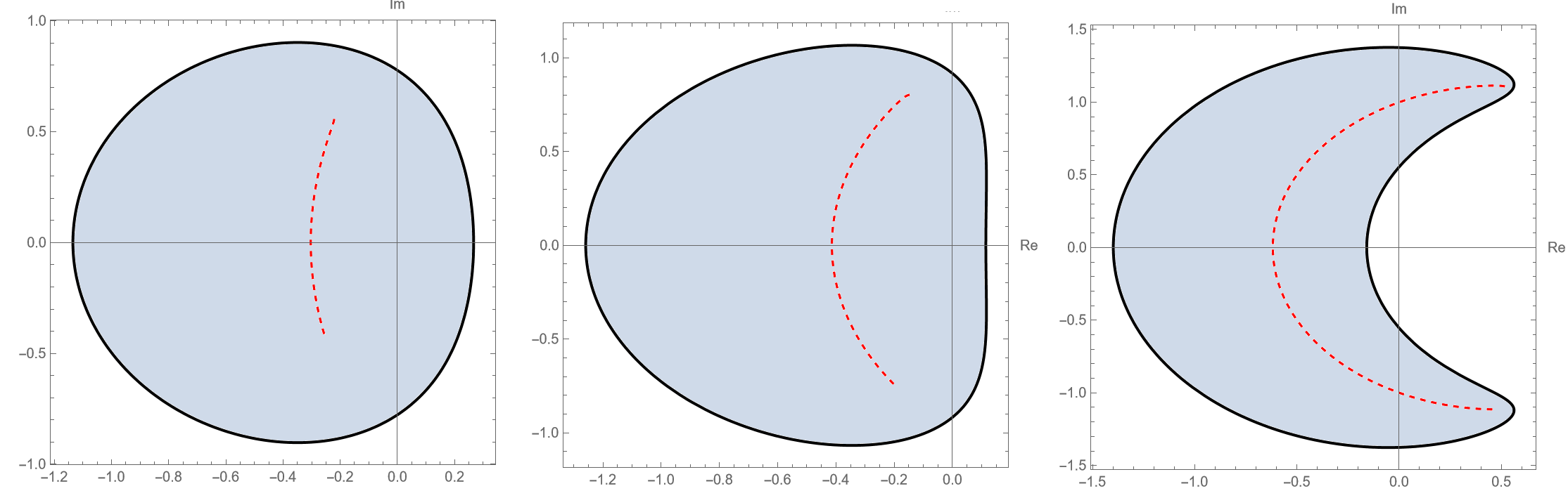
Figure 1: Evolution of the droplet (in shaded blue) and mother body (in dashed red) as $w$ decreases.

Our first result is concerning the mother body (see e.g. the introduction of [9], [31] for contextual and historical remarks). We construct a one-dimensional measure supported on a curve $\Gamma_{0}$ whose Cauchy (also known as Stieltjes) transform agrees with the Cauchy transform of the two-dimensional equilibrium measure on the exterior of $\Omega$.

Theorem 1.1.

There exists a Borel probability measure $\mu_{0}$, supported on a curve $\Gamma_{0}$, which lies in the interior of $\Omega$ and intersects the real line between $(-1/w,0)$ with the following properties:

• There is a rational function $R_{0}$ (explicitly given in (3.18)) such that

  $$d\mu_{0}(s)=\frac{1}{2\pi i}\sqrt{R_{0}(s)}\,ds,$$ (1.23)

  where $ds$ represents the line element of $\Gamma_{0}$. The branch cut of the square root of $R_{0}(s)$ is taken in $\Gamma_{0}$ and the branch is taken such that

  $$\sqrt{R_{0}(z)}=\frac{Q_{0}}{z}+\mathcal{O}(z^{-2}),\quad\text{as }z\to\infty.$$ (1.24)

• There is a smooth simple closed curve $\Gamma$, which has $0$ in its interior and $-1/w$ in its exterior, with $\Gamma_{0}\subset\Gamma$ and a real constant $\ell_{0}$ such that

  $$2U^{\mu_{0}}(z)+\operatorname{Re}\mathcal{V}(z)+\ell_{0}\begin{cases}=0\quad z\in\Gamma_{0},\\ >0\quad z\in\Gamma\setminus\Gamma_{0},\end{cases}$$ (1.25)

  where

  $$\mathcal{V}(z)=(1+Q_{1})\log z+(1+Q_{0})\log\Big{(}z+\frac{1}{w}\Big{)}-Q_{1}\log(z-w).$$ (1.26)

  Here, the branch of the logarithm is chosen on $(-\infty,-1/w]\cup[0,w]$.

• We have the equality of Cauchy transforms

  $$\int\frac{d\nu_{0}(s)}{z-s}=\int\frac{d\mu_{0}(s)}{z-s},\quad z\in\mathbb{C}\setminus\Omega.$$ (1.27)

Remark 1.2.

The measure $\mu_{0}$ can also be characterized as a solution to a max-min equilibrium problem. The steps are given in Appendix A.

To obtain the large $N$ asymptotics of the orthogonal polynomials $P_{n,N}$, we rely on the fact that the planar orthogonality can be reformulated as non-Hermitian contour orthogonality, a fact which is of independent interest.

Proposition 1.3.

Let $N,NQ_{1},NQ_{0}\in\mathbb{N}$. Furthermore, let $P_{n,N}(z)$ satisfy

$$\int_{\mathbb{C}}P_{n,N}(z)\overline{(z-w)}^{k}\frac{|z-w|^{2NQ_{1}}}{(1+|z|^{2})^{N(1+Q_{0}+Q_{1})+1}}\,dA(z)=0,\quad k=0,\dots n-1.$$ (1.28)

Then for a simple closed contour $\Gamma$ with positive orientation which has $0$ in the interior and $-1/w$ in the exterior we have

$$\oint_{\Gamma}P_{n,N}(z)z^{j}(z-w)^{NQ_{1}}\frac{1}{(1+zw)^{N+NQ_{0}}}\frac{1}{z^{n+NQ_{1}}}=0,\quad j=1,\dots n-1.$$ (1.29)

For the orthogonal polynomials associated with the external potential (1.17), the equivalent contour orthogonality was established in [4, §3] and further extended in [40, 6] to the case of multiple point charges. Such contour orthogonality serves as a cornerstone for several works [5, 7, 16, 18, 36, 39, 41, 50] in various asymptotic analyses of orthogonal polynomials, as well as in the study of statistical properties of the associated Coulomb gases. Since (1.17) can be obtained as a particular limit of (1.12) (see [14] for a related discussion), Proposition 1.3 can be regarded as an extension of the result in [4, §3].

Remark 1.4.

From (1.29), the weight function for the non-Hermitian contour orthogonality is given as

$$w_{n,N}(z)=(z-w)^{NQ_{1}}\frac{1}{(z+1/w)^{N+NQ_{0}}}\frac{1}{z^{n+NQ_{1}}}.$$ (1.30)

This matches with $e^{-N\mathcal{V}(z)}$ (recall (1.26) for definition of $\mathcal{V}$) up to a factor $z^{n-N}$ . This will play a crucial role in the steepest descent analysis that follows.

By [26], Proposition 1.3 further allows us to write $P_{n,N}$ as a solution to a $2\times 2$ Riemann-Hilbert problem which is described at the beginning of Section 5, referred to as RH problem 5.1. To obtain the strong asymptotics of $P_{n,N}$ we proceed in Section 5 to perform the Deift-Zhou steepest descent analysis [25] of the Riemann-Hilbert problem, which at a technical level has steps in common with the works [4, 5, 8, 6, 40, 41, 35, 39, 7, 18, 16]. To state our main result about in this regard, we recall the measure $\mu_{0}$ in Theorem 1.1 and its associated $g$-function,

$$g(z)=\int\log(z-s)\,d\mu_{0}(s).$$ (1.31)

Further, we denote the conformal map $F_{1}$ which maps the exterior of the droplet $\Omega$ to the unit disc $\mathbb{D}(0,1)$. It is the inverse of the analytic function $f(u)$ given in (1.21), which behaves as $F_{1}(z)=\rho z^{-1}+\mathcal{O}(z^{-2})$ as $z\rightarrow\infty$.

Theorem 1.5.

Let $w$ satisfy (1.6) and let $n,N\rightarrow\infty$ be such that $n-N=r_{0}<0$ is fixed. Moreover, assume that $N$, $NQ_{1}$, and $NQ_{0}$ are integers. Then we have

$$P_{n,N}(z)=i\Big{(}\frac{\rho}{F_{1}(z)}\Big{)}^{r_{0}}\frac{\sqrt{\rho F_{1}^{\prime}(z)}}{F_{1}(z)}e^{Ng(z)}(1+\mathcal{O}(N^{-1}))\quad\text{as}\hskip 2.84544ptN\rightarrow\infty$$ (1.32)

uniformly for $z$ in compact subsets of $\overline{\mathbb{C}}\setminus\Gamma_{0}$

Remark 1.6.

1. It is expected that the assumptions that $N$, $NQ_{1}$, and $NQ_{0}$ are integers are not essential and that the statement of the theorem holds without them.
2. In (1.32), the pre-factor in front of $e^{Ng(z)}$ appears as the $(1,1)$ entry of the global parametrix 5.8, and the branch cut of $\sqrt{F_{1}^{\prime}(z)}$ is taken such that $i\sqrt{\rho F_{1}^{\prime}(z)}/F_{1}(z)$ tends to $1$ as $z\rightarrow\infty$.
3. The map $F_{1}(z)$ originally defined in $\mathbb{C}\setminus\Omega$ has an analytic continuation to the domain $\mathbb{C}\setminus\Gamma_{0}$. Moreover, we will also see that $F_{1}(z)\neq 0$ and finite valued in $\mathbb{C}\setminus\Gamma_{0}$. This analytic continuation is used in (1.32).
4. The map

$$F_{0}(z)=\frac{1}{F_{1}(z)}:\mathbb{C}\setminus\Omega\rightarrow\mathbb{C}\setminus\mathbb{D}$$ (1.33)

is the conformal map from the exterior of the droplet to the exterior of the unit disc. Then (1.32) can be rewritten as

$$P_{n,N}(z)=\left(\rho F_{0}(z)\right)^{r_{0}}e^{Ng(z)}\sqrt{\rho F_{0}^{\prime}(z)}(1+\mathcal{O}(N^{-1})).$$ (1.34)

The expansion (1.34) is similar to the strong asymptotics of the orthogonal polynomials obtained in [4], and consistent with the known expansion of [33] in the exterior of the droplet.

As a consequence of Theorem 1.5, we obtain the limiting zero counting measure of the polynomials $P_{n,N}$.

Theorem 1.7.

Under the same assumption of Theorem 1.5 all zeros of $P_{n,N}$ tend to $\Gamma_{0}$. In addition, $\mu_{0}$ is the weak limit of the normalized zero counting measure of $P_{n,N}$.

We also obtain the large $N$ expansion of the normalization $h_{n,N}$ in (1.13). Recall $\rho$ in (1.21) and $\ell_{\mathrm{2D}}$ in (1.20).

Theorem 1.8.

Under the same assumption of Theorem 1.5, we have

$$h_{n,N}=\pi\sqrt{\frac{2\pi}{N(Q_{1}+Q_{0}+1)}}\rho^{2r_{0}+1}e^{N\ell_{\mathrm{2D}}}\left(1+\mathcal{O}(N^{-1})\right).$$ (1.35)

Remark 1.9.

1. We find Theorem 1.8 remarkable. The RH problem 5.1 gives us the asymptotics of the normalization of $P_{n,N}$ with respect to the weight $w_{n,N}$, and this involves the Robin constant $\ell_{0}$ in (1.25). However, we can express $\ell_{0}$ in terms of $\ell_{\mathrm{2D}}$ in a curious way, as is done in Lemma 6.1 (a similar miraculous relation also appears in [4, Lemma 7.2]). As we shall see, this drastically simplifies $h_{n,N}$ and gives us (1.35).
2. If (1.35) should be uniformly valid in $r_{0}$ for large $N$, substitution in (1.14) predicts the leading large $N$ asymptotic form

$$\log Q_{N}\sim N^{2}(\ell_{\rm 2D}-\log\rho).$$ (1.36)

Here $Q_{N}$ is the configuration integral associated with (1.11), as given in the LHS of (1.14). Using the identification of $\rho$ in (1.21) as the logarithmic capacity of the droplet (see e.g. [4, text below (1.24)]),

$$\log\rho=\int_{\Omega}d\mu(z)\int_{\Omega}d\mu(w)\,\log|w-z|,$$

we see that (1.36) is consistent with the electrostatic argument of [14, §2.4].

2 Construction of a meromorphic function on a Riemann surface

The map $f$ in (1.21) is a rational map of degree $2$ with poles at $1/a$ and $0$ and zeros at $1/b$ and $\infty$. In addition, the equation $f^{\prime}(u)=0$ admits two complex conjugate solution (due to the fact $a<b$), which are denoted by $u_{1},u_{2}$ and the critical values $f(u_{j})$ are denoted as $z_{j}$. We also note at this stage that the equation $f(z)f(1/z)+1=0$ permits two solutions, $v_{0}$, $1/v_{0}$ both of which are real with $0<v_{0}<1$ and

$$f(v_{0})=w,\qquad f(1/v_{0})=-1/w;$$ (2.1)

see [14, §2.3]

Lemma 2.1.

Each $z_{j}$ lies on the interior of $\Omega$.

Proof.

By symmetry it suffices to consider $z_{1}$. Since $f$ is a twofold branched covering, and the map $f$ is conformal on the interior of the unit disc $\mathbb{D}$, we have $u_{1}\in\mathbb{C}\setminus\mathbb{D}$, and $z_{1}$ has only one preimage $u_{1}$. If $z_{1}$ was in $\mathbb{C}\setminus\Omega$, then since we require $f$ to be surjective from $\mathbb{D}(0,1)$ to $\mathbb{C}\setminus\Omega$, we must have $u_{1}$ in the interior of the unit disc, which is a contradiction.

∎

By definition, the deck transformation, denoted $\mathrm{deck}(u)$, is characterised by the condition that

$$f(u)=f(\mathrm{deck}(u)).$$ (2.2)

Since $f$ is given by (1.21), one can see that

$$\mathrm{deck}(u)=\frac{a-b}{ab}\frac{u}{u-1/b}+\frac{1}{a},$$ (2.3)

and the fixed points of $\mathrm{deck}(u)$ are the critical points of $f$, $u_{1}$ and $u_{2}$. The map $f$ has two inverses denoted by $F_{1}$ and $F_{2}$ which are determined by their behaviour at $\infty$,

$$F_{1}(z)=\frac{\rho}{z}+\mathcal{O}(z^{-2}),\qquad F_{2}(z)=\frac{1}{a}+\mathcal{O}(z^{-1}).$$ (2.4)

In the case of the first of these, $F_{1}$ maps the exterior of the droplet $\Omega$ to the unit disc $\mathbb{D}$ as already noted in the sentence above Theorem 1.5. The two inverses are related by

$$F_{2}(z)=\mathrm{deck}(F_{1}(z)).$$ (2.5)

These inverse functions have the explicit forms

$$F_{1}(z)=\frac{b\rho+z-\sqrt{(z-z_{1})(z-z_{2})}}{2az},$$ (2.6)

$$F_{2}(z)=\frac{b\rho+z+\sqrt{(z-z_{1})(z-z_{2})}}{2az}.$$ (2.7)

The branch cut of the square root is taken as a simple curve $\mathcal{B}$ which joins $z_{1}$ and $z_{2}$ while intersecting the real line between $(-1/w,0)$ once. Moreover, $F_{1}$ has analytic continuation to a second sheet by $F_{2}$ which is connected to the first sheet in a crisscross manner across $\mathcal{B}$. We will in particular make a precise choice of this cut which will turn out to be the mother body.

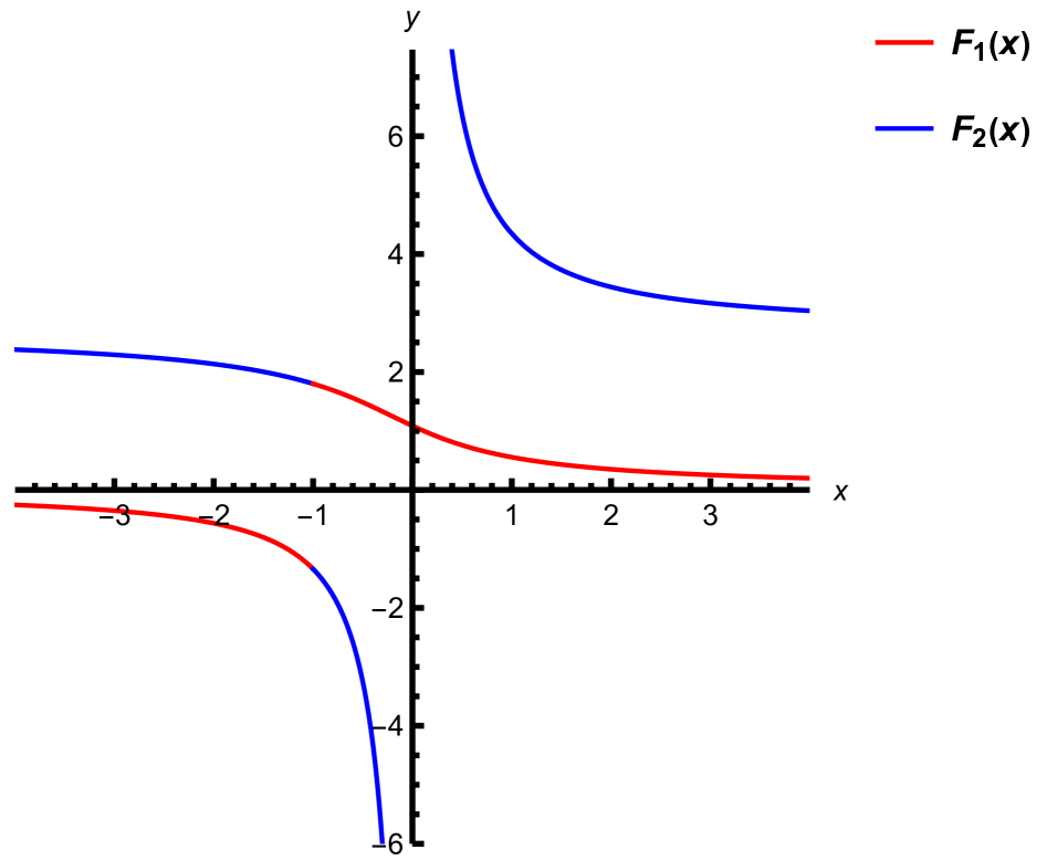
Figure 2: The plot of the function $F_{1}$ in red and its analytic continuation $F_{2}$ in blue on the real line. One observes $F_{2}$ has a pole at $0$.

2.1 Spherical Schwarz function

Denote

$$\nu=\frac{1}{Q_{0}+Q_{1}+1}\nu_{0},$$ (2.8)

where we recall the definition $\nu_{0}$ is the equilibrium measure of (1.19). Applying $\partial_{z}$ to the variational conditions (1.20), we obtain

$$\int\frac{d\nu(s)}{u-s}+\frac{Q_{1}}{1+Q_{0}+Q_{1}}\frac{1}{u-w}=\frac{\overline{u}}{1+|u|^{2}},\qquad u\in\Omega.$$ (2.9)

Since $f$ maps the unit circle to a closed simple curve $\partial\Omega$, we have $F_{1}:\partial\Omega\mapsto\mathbb{S}^{1}.$ Note that if

$$f(u)=z,\qquad|u|=1,\>z\in\partial\Omega,$$ (2.10)

then

$$f(1/F_{1}(z))=f(1/u)=f(\overline{u})=\overline{f(u)}=\overline{z}.$$ (2.11)

Here we have used that the rational map $f$ has real coefficients.

We define

$$S_{1}(z):=\frac{f(1/F_{1}(z))}{1+zf(1/F_{1}(z))},\qquad z\in\mathbb{C}\setminus\mathcal{B}.$$ (2.12)

It is immediate that $S_{1}(z)$ has a pole at $z=w$ with residue $Q_{1}/(1+Q_{0}+Q_{1})$. Also, it is meromorphic in $\mathbb{C}\setminus\mathcal{B}$. From the precedent of [20], we call $S_{1}$ the spherical Schwarz function of the droplet $\Omega$.

We know from [14, Eq. (2.48)] that with $u$ replaced by $f(u)$, $|u|\leq 1$ and thus $f(u)\in\overline{\mathbb{C}\backslash\Omega}$, the RHS of (2.9) can be replaced by the meromorphic function $f(1/u)/(1+f(u)f(1/u))$. Equivalently, we have

$$\int\frac{d\nu(s)}{z-s}+\frac{Q_{1}}{1+Q_{0}+Q_{1}}\frac{1}{z-w}=S_{1}(z),\qquad z\in\overline{\mathbb{C}\backslash\Omega}.$$ (2.13)

One notes from (2.11) that the equality herein for $z\in\Omega$ is consistent with (2.9).

We define the analytic continuation of $S_{1}$ across the branch cut $\mathcal{B}$ (the precise form is yet to be chosen) joining $z_{1},z_{2}$ by the map $F_{2}$ as

$$S_{2}(z):=\frac{f(1/F_{2}(z))}{1+zf(1/F_{2}(z))}.$$ (2.14)

Then defining $\mathcal{R}$ to be a two-sheeted Riemann surface with sheets $\mathcal{R}_{j}$ ($j=1,2$), the map

$$S(z):=\begin{cases}S_{1}(z)\quad z\in\mathcal{R}_{1},\\ S_{2}(z)\quad z\in\mathcal{R}_{2},\end{cases}$$ (2.15)

defines a meromorphic function on $\mathcal{R}$; see Figure 3.

Figure 3: The Riemann surface $\mathcal{R}$

We now determine its poles, zeros and an underlying algebraic equation. From the asymptotic behaviour given by (2.4), it is easy to see that

$$S_{1}(z)=\frac{b\rho^{2}}{z\left(a+b\rho^{2}\right)}+\mathcal{O}(z^{-2})=\frac{Q_{1}+1}{Q_{0}+Q_{1}+1}\frac{1}{z}+\mathcal{O}(z^{-2}),\qquad z\to\infty.$$ (2.16)

An alternative derivation is to recall that $S_{1}(z)$ has a pole at $z=w$ with residue $Q_{1}/(1+Q_{0}+Q_{1})$, and to note that by (2.8), the Cauchy transform of the droplet measure satisfies

$$\int\frac{d\nu(s)}{z-s}=\frac{1}{Q_{0}+Q_{1}+1}\frac{1}{z}+\mathcal{O}(z^{-2}),\qquad z\to\infty.$$

In addition, by (2.4), we have

$$S_{2}(z)=\frac{1}{z}+\mathcal{O}(z^{-2}),\qquad z\to\infty.$$ (2.17)

Due to the fact $F_{2}(z)$ has a pole at 0 (as it should as $f$ maps $\infty$ to zero), we have by residue calculation that

$$S_{2}(z)=\frac{Q_{1}+1}{1+Q_{0}+Q_{1}}\frac{1}{z}+\mathcal{O}(z^{-2}),\qquad z\to 0.$$ (2.18)

Remark 2.2.

Note that $f$ has a pole at $1/a$ and therefore $1/F(f(a))=1/a$ at $f(a)$, telling us that $S$ has an isolated singularity at $f(a)$. However, due to the pole appearing in the numerator and denominator together in (2.14), the singularity is removable.

Recall (2.1). Since the sum of residues of a meromorphic function $S_{2}$ (viewed on the Riemann surface $\mathcal{R}$) should vanish, it follows from (2.14), (2.18), (2.16), (2.17) and (2.9) that $S_{2}$ has a pole at $-1/w$ with residue $(1+Q_{0})/(1+Q_{0}+Q_{1})$.

Lemma 2.3.

There exists $c_{0}$, with $c_{0}>w$, such that $S_{1}(c_{0})=S_{2}(c_{0})$.

Proof.

We first observe that $S_{1},S_{2}$ are real and analytic in $(w,\infty)$. In addition, $S_{1}$ has a pole at $w$, with a positive residue, giving us $S_{1}(s)>S_{2}(s)$ for $s\in(w,w+\varepsilon)$, with $\varepsilon>0$ sufficiently small. Next, from (2.16) and (2.17) we can conclude $S_{2}(s)>S_{1}(s)$ for sufficiently large $s$. The proof is then complete, invoking the intermediate value theorem. ∎

2.2 Spectral Curve

With the knowledge in the previous subsection, we are ready to determine the underlying algebraic curve, referred to as the spectral curve. The symmetric functions of the branches of a meromorphic function are rational; hence, we have $S_{1}+S_{2}$ and $S_{1}S_{2}$ are rational functions. Define,

$$\begin{split}P_{1}(z)&:=S_{1}(z)+S_{2}(z)\\ &=\frac{1+Q_{0}}{1+Q_{0}+Q_{1}}\frac{1}{z+1/w}+\frac{Q_{1}}{1+Q_{0}+Q_{1}}\frac{1}{z-w}+\frac{Q_{1}+1}{1+Q_{0}+Q_{1}}\frac{1}{z},\end{split}$$ (2.19)

and

$$P_{2}(z):=S_{1}(z)S_{2}(z)=\frac{Q_{1}+1}{1+Q_{0}+Q_{1}}\frac{z-f(b)}{(z-w)(z+1/w)z}.$$ (2.20)

Here, to evaluate the coefficients in (2.20), we have used the asymptotic behaviours (2.16) and (2.17), as well as the fact that $S$ has a zero at $f(b)$ by construction (2.12), (2.14), (2.11) and (1.21).

Hence we have determined the spectral curve completely, as specified by

$$P(S,z)=S^{2}+P_{1}(z)S+P_{2}(z)=0,$$ (2.21)

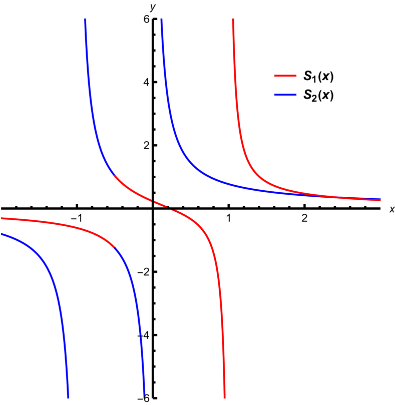
Figure 4: The Schwarz function $S_{1}$ and $S_{2}$ on the real axis. One can observe three poles, one zero and a node at the real axis.

where $P_{1}(z)$ and $P_{2}(z)$ are given by the RHS of (2.19) and $\eqref{P2}$.

Remark 2.4.

$P(S,z)$ is not symmetric in $S,z$. In $S$ it has degree 2, while in $z$ degree 3.

We now write the rational function

$$R(z):=P_{1}(z)^{2}-4P_{2}(z)$$ (2.22)

for the discriminant of the algebraic curve (2.21). Completing the square in (2.21) we have

$$\Big{(}S-\frac{P_{1}(z)}{2}\Big{)}^{2}=\frac{1}{4}R(z).$$ (2.23)

By (2.23), we obtain

$$S_{2}(z)-\frac{P_{1}(z)}{2}=\frac{1}{2}\sqrt{R(z)},\qquad S_{1}(z)-\frac{P_{1}(z)}{2}=-\frac{1}{2}\sqrt{R(z)}.$$ (2.24)

In the above and what follows the branch cut of $\sqrt{R(z)}$ is taken to be $\mathcal{B}$ (the same branch cut of $F_{1}$ defined in (2.6)), and we also have for this branch that as $z\rightarrow\infty$,

$$\sqrt{R(z)}=\frac{Q_{0}}{1+Q_{0}+Q_{1}}\frac{1}{z}+\mathcal{O}(z^{-2});$$ (2.25)

see (2.16), (2.17) and (2.19). In addition, it follows from (2.24) that

$$R(z)=(S_{1}(z)-S_{2}(z))^{2}.$$ (2.26)

We can make $R(z)$ more explicit. By using (2.16), (2.17), (2.19), (2.20) and (2.22), we have

$$R(z)=\Big{(}\frac{Q_{0}}{1+Q_{0}+Q_{1}}\Big{)}^{2}\frac{1}{z^{2}}+\mathcal{O}(z^{-3}),\quad z\rightarrow\infty.$$ (2.27)

Also, we have $R(z)$ to be a rational function with double poles at $w,-1/w,0$. Hence, it must be that

$$R(z)=\frac{P_{4}(z)}{(z-w)^{2}(z+1/w)^{2}z^{2}},$$ (2.28)

where $P_{4}(z)$ is a quartic polynomial. We determine its zeros. As we observed that $R(z)$ coincides with the discriminant of the spectral curve, the zeros occur when $S_{1}(z)=S_{2}(z)$. Two solutions are evidently the branch points $z_{1},z_{2}$. Further Lemma 2.3 gives us $c_{0}$ is a double zero. Thus we have

$$R(z)=\Big{(}\frac{Q_{0}}{1+Q_{0}+Q_{1}}\Big{)}^{2}\frac{(z-z_{1})(z-z_{2})(z-c_{0})^{2}}{(z-w)^{2}(z+1/w)^{2}z^{2}},$$ (2.29)

where $z_{1},z_{2}$ are given as the critical values of the conformal map $f$ and $c_{0}$ is a multiple zero of $\mathrm{Disc}(P(S,z),S)$. In regards to this, we also have from (2.24) that

$$R(z)=\Big{(}S_{2}(z)-\frac{P_{1}(z)}{2}\Big{)}^{2}$$ (2.30)

and $S_{2}(z)$ has a pole at $0$ with residue $(Q_{1}+1)/(Q_{0}+Q_{1}+1)$. By comparing the leading-order coefficient of $1/z^{2}$ in the two expressions for $R$ as $z\to 0$, and using (2.18), (2.19), along with the relation $z_{2}=\overline{z}_{1}$, we obtain

$$c_{0}=\frac{1+Q_{1}}{Q_{0}}\frac{1}{|z_{1}|}.$$ (2.31)

Next we make note of a particular property relating to $c_{0}$ which will be required in subsequent working.

Lemma 2.5.

Suppose

$$S_{1}(z)=\frac{\overline{z}}{1+|z|^{2}}\qquad\text{for }z\notin\partial\Omega.$$ (2.32)

Then $z=c_{0}$.

Proof.

Let $z=f(v)$. Then by (2.12) the condition (2.32) is rewritten as

$$\frac{f(1/v)}{1+f(v)f(1/v)}=\frac{f(\overline{v})}{1+f(v)f(\overline{v})}.$$ (2.33)

Simplifying shows

$$f(1/v)=f(\overline{v}),$$ (2.34)

which means

$$\mathrm{deck}(v)=1/\overline{v},$$ (2.35)

where we have used (2.2). Therefore we have

$$S_{1}(z)=\frac{f(1/v)}{1+f(1/v)f(v)}=\frac{f(\overline{v})}{1+f(v)f(\overline{v})}=\frac{f(1/\mathrm{deck}(v))}{1+f(1/\mathrm{deck}(v))f(v)}=S_{2}(z),$$ (2.36)

which implies $z=z_{1}$ or $z_{2}$ or $c_{0}$ by the discussion above (2.29). Since $u_{1}$ and $u_{2}$ are fixed points of $\mathrm{deck}(u)$, it follows that if $z=z_{k}$ for $k=1$ or $2$, by (2.35), $|u_{k}|=1$, which implies that $z\in\partial\Omega$. Hence, $z$ must be $c_{0}$. ∎

Recall (1.20) for the definition of $\mathcal{U}_{\mathrm{2D}}$. As a corollary, we observe that $c_{0}$ is the only critical point of $\mathcal{U}_{\mathrm{2D}}$ in $\mathbb{C}\setminus\Omega$.

Lemma 2.6.

The inequality in (1.20) is strict. That is

$$\mathcal{U}_{2D}(z)>0,\quad z\in\mathbb{C}\setminus\Omega.$$ (2.37)

Proof.

By (1.20) we find $\partial\mathcal{U}_{2D}=\overline{\partial}\mathcal{U}_{2D}=0$ on $\Omega$. Assume that there is a local minimum of $\mathcal{U}_{2D}$ on $\mathbb{C}\setminus\Omega$. Then the Mountain Pass Theorem guarantees that there is a critical point on a path connecting $\Omega$ and the local minimum. By (2.13), one can notice that $\partial\mathcal{U}_{2D}$ is equivalent to the condition (2.32). On the other hand, by Lemma 2.5 there is at most one critical point in $\mathcal{U}_{2D}$, therefore there is no local minimum of $\mathcal{U}_{2D}$ on $\mathbb{C}\setminus\Omega$. ∎

3 The mother body

In this section Theorem 1.1 will be established.

3.1 Analysis of the trajectories of the quadratic differential

We are interested in the trajectories of the quadratic differential

$$R(z)\,dz^{2}<0.$$

This in essence will give us a real measure $\mu$ with density

$$d\mu(z)=\frac{1}{2\pi i}\sqrt{R(z)}\,dz,$$

supported on the critical trajectories. Here, $dz$ represents the complex line element.

We recall from (2.29) and (2.31)

$$R(z)=\Big{(}\frac{Q_{0}}{1+Q_{0}+Q_{1}}\Big{)}^{2}\frac{(z-z_{1})(z-z_{2})(z-c_{0})^{2}}{z^{2}(z-w)^{2}(z+1/w)^{2}},\qquad c_{0}=\frac{1+Q_{1}}{Q_{0}}\frac{1}{|z_{1}|}.$$ (3.1)

In that regard, we have the meromorphic differential

$$(S_{1}(z)-S_{2}(z))^{2}\,dz^{2}=R(z)\,dz^{2}.$$

By general theory [34, 45, 48, 49], we have the following rules for the trajectories of the quadratic differential $R(z)\,dz^{2}<0$.

• $z_{1},z_{2}$ are simple zeros of $R(z)$. Hence, there are three equiangular arcs emanating from $z_{1}$ and $z_{2}$.

• $c_{0}$ is a double zero of $R(z)$. Therefore, there are four equiangular arcs emanating from $c_{0}$.

• $0,w,-1/w$ are double poles with positive residues. Hence, the trajectories near $0,w,-1/w$ are locally circular.

• $R(z)\sim z^{-2}$, as a result, infinity is a double pole with positive residue. Then the trajectories near infinity are also circular, that is closed loops.

• We use the weak version of Teichmüller’s Lemma: a simply connected domain bounded by critical trajectories that does not contain a pole on its boundary must have a pole in its interior.

• By symmetry, if $\gamma$ is a trajectory, then so is $\overline{\gamma}$.

Due to item (4), the short critical trajectories are finite and do not escape to infinity. Consequently, the trajectories emanating from $z_{1}$ in the upper half-plane must terminate at either $z_{2}$ or $c_{0}$. Moreover, at most one of these three trajectories can end at $c_{0}$, as ensured by items (5) and (6).

In the following, we show all the critical trajectories emanating from $z_{1}$ terminate at $z_{2}$.

3.1.1 Potential theoretic preliminaries

We begin with some definitions.

Definition 3.1.

For $z\in\mathbb{C}\setminus\mathcal{B}$, define

$$\mathcal{U}(z):=\log(1+|z|^{2})-\log(1+|z_{0}|^{2})-2\operatorname{Re}\int_{z_{0}}^{z}S_{1}(s)\,ds,$$ (3.2)

where the contour of integration is away from the branch cut $\mathcal{B}$ and $z_{0}$ is in $\partial\Omega$.

Notice that by (1.20) and (2.13),

$$\mathcal{U}_{2D}(z)=(Q_{0}+Q_{1}+1)\mathcal{U}(z),\qquad z\in\overline{\mathbb{C}\backslash\Omega}.$$

Next, we define an indefinite integral with $\sqrt{R(s)}$ as the integrand.

Definition 3.2.

For $z\in\mathbb{C}\setminus\mathcal{B}$, define

$$\mathcal{U}_{0}(z):=\operatorname{Re}\int_{z_{1}}^{z}\sqrt{R(s)}\,ds,$$ (3.3)

where the contour of integration is in $\mathbb{C}\setminus\mathcal{B}$.

Recall that $c_{0}$ is defined in Lemma 2.3 and is given by the expression in (2.31).

Proposition 3.3.

We have

$$\mathcal{U}_{0}(c_{0})=\mathcal{U}(c_{0})>0.$$

Proof.

The last inequality is an easy consequence of Lemma 2.6 combining with Lemma 2.3 which tells us $c_{0}\in\mathbb{C}\setminus\Omega$. We prove the first equality. Let us denote $F_{1}(c_{0})=v$. Then by (2.35) we have $\mathrm{deck}(1/v)=\overline{v}$. Then by (2.26), (2.12), (2.14) and (2.5), we have

$$\begin{split}&\quad 2\int_{z_{1}}^{c_{0}}\sqrt{R(s)}\,ds=2\int_{z_{1}}^{c_{0}}(S_{2}(s)-S_{1}(s))\,ds\\ &=2\int_{u_{1}}^{v}\frac{f(1/\mathrm{deck}(u))}{1+f(1/\mathrm{deck}(u))f(u)}d(f(\mathrm{deck}(u)))-2\int_{u_{1}}^{v}\frac{f(1/u)}{1+f(1/u)f(u)}d(f(u))\\ &=2\int_{v}^{\mathrm{deck}(v)}\frac{f(1/u)}{1+f(1/u)f(u)}d(f(u)).\end{split}$$ (3.4)

Let $z_{0}\in\partial\Omega$ and $v_{0}\in\partial\mathbb{D}$ such that $f(v_{0})=z_{0}$. We decompose the last integral as $A_{1}+B_{1}$, where

$$A_{1}:=\int_{v}^{v_{0}}\frac{f(1/u)}{1+f(1/u)f(u)}d(f(u)),\qquad B_{1}:=\int_{v_{0}}^{\mathrm{deck}(v)}\frac{f(1/u)}{1+f(1/u)f(u)}d(f(u)).$$

Notice that by definition (2.12), we have

$$A_{1}=-\int_{z_{0}}^{c_{0}}S_{1}(s)\,ds.$$ (3.5)

On the other hand, we have

$$\begin{split}B_{1}&=\int_{v_{0}}^{\mathrm{deck}(v)}d\log(1+f(1/u)f(u))+\frac{f(u)f^{\prime}(1/u)}{u^{2}(1+f(1/u)f(u))}\,du\\ &=\Big{[}\log(1+f(1/u)f(u))\Big{]}_{v_{0}}^{\mathrm{deck}(v)}+\int_{1/\mathrm{deck}(v)}^{1/v_{0}}\frac{f(1/x)f^{\prime}(x)}{1+f(1/x)f(x)}\,dx\\ &=\log(1+|c_{0}|^{2})-\log(1+|z_{0}|^{2})-\int^{\overline{c}_{0}}_{\overline{z}_{0}}S_{1}(x)\,dx.\end{split}$$ (3.6)

Combining all of the above, we obtain

$$\quad 2\mathcal{U}_{0}(c_{0})=2\operatorname{Re}\int_{z_{1}}^{c_{0}}\sqrt{R(s)}\,ds=2\operatorname{Re}(A_{1}+B_{1})$$ (3.7)

$$=2\log(1+|c_{0}|^{2})-2\log(1+|z_{0}|^{2})-2\operatorname{Re}\int^{\overline{c}_{0}}_{\overline{z}_{0}}S_{1}(x)\,dx-2\operatorname{Re}\int_{z_{0}}^{c_{0}}S_{1}(s)\,ds$$

$$=\mathcal{U}(c_{0})+\mathcal{U}(\overline{c}_{0})=2\mathcal{U}(c_{0})$$

This finishes the proof. ∎

We have seen that the three equiangular trajectories emanating from $z_{1}$ must all terminate at $z_{2}$, forming two simply connected domains, $\tilde{\Omega}_{1}$ and $\tilde{\Omega}_{2}$, each containing at least one pole. By Teichmüller’s Lemma [48, Appendix], if a domain $\tilde{\Omega}_{j}$ contains two poles, it must also contain two zeros (counted with multiplicty, hence in this case it must contain $c_{0}$). This reduces to two cases:

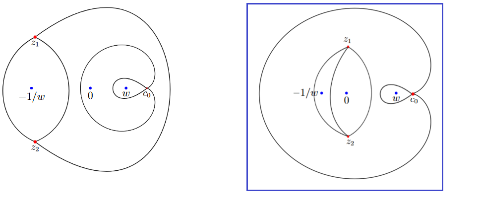
Figure 5: Possible topological configuration of critical trajectories. Case I in left, Case II (in box) in right which satisfies the inequality in Proposition 3.3.

• Case I: $\tilde{\Omega}_{1}$ contains $0,w$ and $c_{0}$, while $\tilde{\Omega}_{2}$ contains $-1/w$. This corresponds left panel of Figure 5.

• Case II: $\tilde{\Omega}_{1}$ contains $0$ and $\tilde{\Omega}_{2}$ contains $-1/w$. This corresponds to right panel of Figure 5.

We now negate Case I. Since we have $\sqrt{R(x)}>0$ for $x>c_{0}$ and $\sqrt{R(x)}<0$ for $x\in(w,c_{0})$. Then $\int_{x}^{c_{0}}\sqrt{R(s)}ds<0$ for $x\in(w,\infty)$ and $x\neq c_{0}$. Suppose Case I is taking place; then we have a trajectory (part of the boundary of $\Omega_{1}$) emanating from $z_{1}$ intersecting the real line at $x_{0}$ with $x_{0}>c_{0}$. Then one observes

$$\operatorname{Re}\int_{z_{1}}^{c_{0}}\sqrt{R(s)}\,ds=\operatorname{Re}\int_{z_{1}}^{x_{0}}\sqrt{R(s)}\,ds+\operatorname{Re}\int^{c_{0}}_{x_{0}}\sqrt{R(s)}\,ds<0.$$ (3.8)

This contradicts Proposition 3.3.

As a corollary, we obtain the following.

Corollary 3.4.

• All the three equiangular arcs emanating from $z_{1}$ terminates at $z_{2}$. These form two simply connected domains, $\tilde{\Omega}_{1}$ (containing $0$) and $\tilde{\Omega}_{2}$ (containing $-1/w$).

• From $c_{0}$, emanates four equiangular arcs, forming two loops, one enclosing $w$ and one enclosing all the poles $-1/w,0,w$.

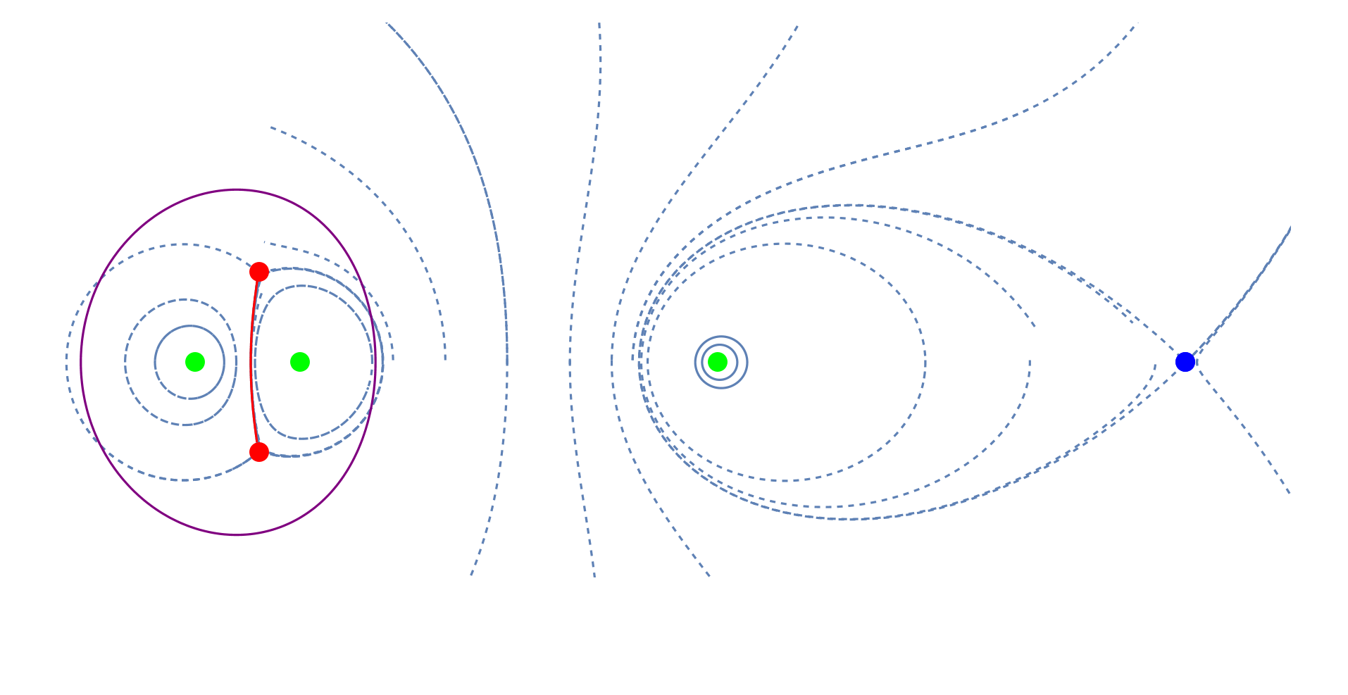
Figure 6: Global structure of trajectories of the quadratic differential $(S_{1}(z)-S_{2}(z)^{2}dz^{2}$: mother body in red, droplet in purple, poles in green, node in blue dots.

This finishes the discussion on the trajectories of the quadratic differential and confirms the numerical simulation in Figure 6.

Lemma 3.5.

The steepest ascent path $\Gamma_{1}$ of $\mathcal{U}_{0}$ from $z_{1}$ terminates at $c_{0}$ and similarly the steepest ascent path $\Gamma_{2}$ of $\mathcal{U}_{0}$ from $z_{2}$ terminates at $c_{0}$. Moreover, we have $\mathcal{U}_{0}(z)>0$ for $z\in\Gamma_{j}$, where $j=1,2$.

Proof.

The proof follows in the same line as that of [4, Lemma 3.3, Appendix C]. That is, if $v=F_{1}(z)$ satisfies $\mathrm{deck}(v)=1/\overline{v}$, then LHS of (3.4) is purely real. Since $c_{0}$ is such a point, we have $\int_{z_{1}}^{c_{0}}\sqrt{R(s)}ds=\mathcal{U}(c_{0})>0$. Thus, $c_{0}$ lies on the steepest ascent path from $z_{1}$. By symmetry we can conclude the same about $\Gamma_{2}$. See also Figure 7 for numerical confirmation. ∎

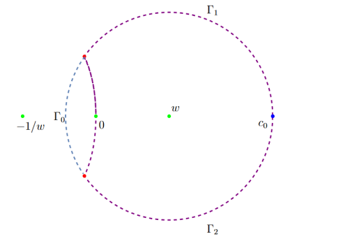
Figure 7: The contour $\Gamma=\Gamma_{0}\cup\Gamma_{1}\cup\Gamma_{2}$. The steepest ascent path $\Gamma_{1}$ and $\Gamma_{2}$ in dashed purple. $\Gamma_{0}$ in dashed blue.

3.2 Proof of Theorem 1.1

Definition 3.6.

Define $\Gamma_{0}$ as the unique trajectory of the quadratic differential $R(z)\,dz^{2}<0$ emanating from $z_{1}$ and terminating at $z_{2}$ which intersects the real line between $-1/w,0$ which is guaranteed by Corollary 3.4. Further, define

$$d\mu(s):=\frac{1}{2\pi i}\sqrt{R(s)}\,ds,\quad s\in\Gamma_{0}.$$ (3.9)

We are now ready to prove Theorem 1.1.

Proof of Theorem 1.1.

According to Definition 3.6, $\mu$ is a real measure supported on $\Gamma_{0}$, with a density that vanishes as a square root at $z_{1}$ and $z_{2}$, while remaining strictly positive in the interior.

Now choosing the branch cut $\mathcal{B}$ to be exactly on $\Gamma_{0}$ we obtain

$$\frac{1}{2\pi i}\left(S_{1,-}(z)-S_{1,+}(z)\right)dz=d\mu(z),\quad z\in\Gamma_{0}.$$ (3.10)

Then we obtain by the residue theorem,

$$\int\frac{d\mu(s)}{z-s}=\frac{1}{2\pi i}\int_{\Gamma_{0}}\frac{S_{1,-}(s)-S_{1,+}(s)}{z-s}\,ds=S_{1}(z)-\frac{Q_{1}}{1+Q_{0}+Q_{1}}\frac{1}{z-w}.$$ (3.11)

A similar calculation shows

$$S_{1}(z)=\int\frac{d\mu(s)}{z-s}+\frac{Q_{1}}{1+Q_{0}+Q_{1}}\frac{1}{z-w},$$ (3.12)

$$S_{2}(z)=-\int\frac{d\mu(s)}{z-s}+\frac{1+Q_{1}}{1+Q_{0}+Q_{1}}\frac{1}{z}+\frac{1+Q_{0}}{1+Q_{0}+Q_{1}}\frac{1}{z+1/w}.$$

By comparing the behaviour at $\infty$ in the LHS and RHS of (3.12) using (2.16) and (2.17), we obtain

$$\mu(\mathbb{C})=\frac{1}{1+Q_{0}+Q_{1}}.$$ (3.13)

In what follows we will denote,

$$C^{\mu}(z)=\int\frac{d\mu(s)}{z-s},\qquad z\in\mathbb{C}\setminus\mathrm{supp}(\mu).$$ (3.14)

Putting (3.12) and (2.19) in (2.23), we obtain

$$\bigg{(}C^{\mu}(z)+\frac{1}{2}\Big{(}\frac{Q_{1}}{1+Q_{0}+Q_{1}}\frac{1}{z-w}-\frac{1+Q_{0}}{1+Q_{0}+Q_{1}}\frac{1}{z+1/w}-\frac{Q_{1}+1}{1+Q_{0}+Q_{1}}\frac{1}{z}\Big{)}\bigg{)}^{2}=\frac{1}{4}R(z).$$ (3.15)

Also, it is convenient to define the scaling of $\mu$ and $R$. Thus for $\mu$ defined in (3.6) we introduce the scaled form

$$\mu_{0}=(1+Q_{0}+Q_{1})\mu.$$ (3.16)

Then due to (3.13) we have $\mu_{0}$ to be a probability measure supported on $\Gamma_{0}$. That is

$$\mu_{0}(\mathbb{C})=1.$$ (3.17)

In relation to $R$ we define the scaled form

$$R_{0}(z)=(1+Q_{0}+Q_{1})^{2}R(z),$$ (3.18)

and we introduce too

$$\tilde{\mathcal{U}}(z)=(1+Q_{0}+Q_{1})\mathcal{U}(z),\qquad\tilde{\mathcal{U}}_{0}(z)=(1+Q_{0}+Q_{1})\mathcal{U}_{0}(z).$$ (3.19)

This then establishes item (1) in Theorem 1.1, where we have also used (2.25).

Next, we verify item (2). For this, recall from definition (1.26),

$$\mathcal{V}(z)=(1+Q_{1})\log z+(1+Q_{0})\log\Big{(}z+\frac{1}{w}\Big{)}-Q_{1}\log(z-w),$$ (3.20)

where the branch of the logarithm is chosen on $(-\infty,-1/w]\cup[0,w]$. Then (3.15) can be rewritten as

$$\Big{(}C^{\mu_{0}}(z)-\frac{1}{2}\mathcal{V}^{\prime}(z)\Big{)}^{2}=\frac{1}{4}R_{0}(z).$$ (3.21)

Recall $\Gamma_{1}$ and $\Gamma_{2}$ from Lemma 3.5. Now we are ready to define the contour

$$\Gamma=\Gamma_{0}\cup\Gamma_{1}\cup\Gamma_{2},$$ (3.22)

which is a closed contour enclosing $0$ and has $-1/w$ on the exterior. From (3.21) and Lemma 3.5 integrating in $z$ and taking the real part, we obtain that there exists a real constant $\ell_{0}$ such that

$$2U^{\mu_{0}}(z)+\operatorname{Re}\mathcal{V}(z)+\ell_{0}\begin{cases}=0\quad z\in\Gamma_{0},\\ >0\quad z\in\Gamma\setminus\Gamma_{0}.\end{cases}$$ (3.23)

This establishes item (2) of Theorem 1.1.

For item (3), we first note that $\mathcal{B}=\Gamma_{0}\subset\Omega$. We do not provide a proof of this, as it is identical to that of [4, Lemma 2.8]. As a consequence, by comparing (3.12) and (2.12), we obtain (1.27). This establishes item (3) of Theorem 1.1. ∎

Remark 3.7.

It also follows from (3.21) and (1.25) that the contour $\Gamma_{0}$ is a S curve (See [43,  Lemma 5.4]. That is we have,

$$\frac{\partial}{\partial n_{+}}\left(2U^{\mu_{0}}(z)+\operatorname{Re}\mathcal{V}(z)\right)=\frac{\partial}{\partial n_{-}}\left(2U^{\mu_{0}}(z)+\operatorname{Re}\mathcal{V}(z)\right),\quad z\in\Gamma_{0},$$ (3.24)

where $n_{\pm}$ are the unit normal vectors to $\Gamma_{0}$ at $z$. This S property has appeared in several works such as [37, 46, 44].

4 Contour Orthogonality

Crucial to our subsequent Riemann-Hilbert analysis is that the planar orthogonality relation with respect to the weight $e^{-NV(z)}$, with $V(z)$ given by (1.12), is proportional to a non-Hermitian contour orthogonality with weight function (1.30).

Lemma 4.1.

Let $N,NQ_{1},NQ_{0}\in\mathbb{N}$. Further, let $j,k\leq N$. We have

$$\quad\int_{\mathbb{C}}z^{j}\overline{(z-w)}^{k}|z-w|^{2NQ_{1}}\Big{(}\frac{1}{1+|z|^{2}}\Big{)}^{N(1+Q_{0}+Q_{1})+1}\,dA(z)$$ (4.1)

$$=G_{k,N}\oint_{\Gamma}z^{j}(z-w)^{NQ_{1}}\Big{(}\frac{1}{1+wz}\Big{)}^{N+NQ_{0}-k}\Big{(}\frac{1}{z}\Big{)}^{k+1+NQ_{1}}\,dz,$$

where $\Gamma$ is a simple closed contour with positive orientation and has $0$ on the interior and $-1/w$ on the exterior and

$$G_{k,N}:=\frac{\Gamma(N+NQ_{0}-k)\Gamma(1+k+NQ_{1})}{2i\,\Gamma(N(1+Q_{0}+Q_{1})+1)}.$$ (4.2)

Remark 4.2.

Before the proof, let us consider the special case $w=0$ of the formula (4.1). For $w=0$, the LHS of (4.1) can be evaluated using polar coordinates and Euler’s beta integral as

$$\int_{\mathbb{C}}\frac{z^{j}\overline{z}^{k}|z|^{2NQ_{1}}}{(1+|z|^{2})^{N(1+Q_{0}+Q_{1})+1}}\,dA(z) =2\pi\int_{0}^{\infty}\frac{r^{2k+2NQ_{1}+1}}{(1+r^{2})^{N(1+Q_{0}+Q_{1})+1}}\,dr\,\delta_{j,k}=2\pi i\,G_{k,N}\,\delta_{j,k}.$$

On the other hand, the integral in the RHS of (4.1) is evaluated as

$$\oint_{\Gamma}z^{j-k-1}\,dz=2\pi i\,\delta_{j,k}.$$

Thus one can directly observe that (4.1) holds for $w=0$.

Proof of Lemma 4.1.

Consider the integral

$$\int_{\mathbb{C}}z^{j}\overline{(z-w)}^{k}|z-w|^{2NQ_{1}}\Big{(}\frac{1}{1+|z|^{2}}\Big{)}^{N(1+Q_{0}+Q_{1})+1}\,dA(z).$$ (4.3)

Following [4], we denote

$$\chi(z):=(z-w)^{NQ_{1}}\int_{w}^{\overline{z}}(s-w)^{NQ_{1}+k}\Big{(}\frac{1}{1+zs}\Big{)}^{N(Q_{1}+Q_{0}+1)+1}\,ds.$$ (4.4)

Then we have

$$\overline{\partial}_{z}\chi(z)=\overline{(z-w)^{k}}|z-w|^{2NQ_{1}}\Big{(}\frac{1}{1+|z|^{2}}\Big{)}^{N(1+Q_{0}+Q_{1})+1}.$$ (4.5)

Clearly $\chi(z)$ is smooth in $\mathbb{C}\setminus\{-1/w\}$ due to the assumption that $N,NQ_{1},NQ_{0}\in\mathbb{N}$. Also, the integrand in (4.4) has a pole at $-1/z$, however, it is easy to see, that the residue is $0$, hence (4.4) does not depend on the choice of contour.

Let $\varepsilon>0$ be sufficiently small. For $z\notin(\mathbb{D}(-1/w,\varepsilon)\cup\{0\})$ we divide the integral in (4.4) in two parts

$$\int_{w}^{\overline{z}}(s-w)^{NQ_{1}+k}\Big{(}\frac{1}{1+zs}\Big{)}^{N(Q_{1}+Q_{0}+1)+1}\,ds=\mathcal{A}_{1}(z)+\mathcal{B}_{1}(z),$$ (4.6)

where

$$\mathcal{A}_{1}(z):=\int_{w}^{\overline{z}\times\infty}(s-w)^{NQ_{1}+k}\Big{(}\frac{1}{1+zs}\Big{)}^{N(Q_{1}+Q_{0}+1)+1}\,ds,$$

and

$$\mathcal{B}_{1}(z) :=-\int_{\overline{z}}^{\overline{z}\times\infty}(s-w)^{NQ_{1}+k}\Big{(}\frac{1}{1+zs}\Big{)}^{N(Q_{1}+Q_{0}+1)+1}\,ds$$

$$=-\overline{z}\int_{1}^{\infty}(t\overline{z}-w)^{NQ_{1}+k}\Big{(}\frac{1}{1+|z|^{2}t}\Big{)}^{N(Q_{1}+Q_{0}+1)+1}\,dt.$$

Thus $\mathcal{B}_{1}(z)$ is continuous away from $0$, in particular in a neighborhood of $-1/w$.

For $k<N$ and for $|z|>R$ we have for $R$ sufficiently large

$$|\mathcal{B}_{1}(z)|=\mathcal{O}\Big{(}\frac{1}{(1+|z|)^{2NQ_{0}+NQ_{1}+N}}\Big{)}.$$ (4.7)

Due to continuity of $\mathcal{B}_{1}(z)$, for $z\in\mathbb{D}(-1/w,2\varepsilon)$, where $\varepsilon>0$ is sufficiently small, there is a constant $C_{1}>0$ independent of $\varepsilon$, such that

$$|\mathcal{B}_{1}(z)|\leq C_{1}.$$ (4.8)

For the quantity $\mathcal{A}_{1}$, we have a remarkable exact evaluation in terms of gamma functions. For this, note that

$$\mathcal{A}_{1}(z) =\int_{0}^{\overline{z}\times\infty}t^{NQ_{1}+k}\Big{(}\frac{1}{1+wz+zt}\Big{)}^{N(Q_{1}+Q_{0}+1)+1}\,dt$$

$$=\Big{(}\frac{1}{1+wz}\Big{)}^{N(Q_{1}+Q_{0}+1)+1}\int_{0}^{\overline{z}\times\infty}t^{NQ_{1}+k}\Big{(}1+\frac{z}{1+wz}t\Big{)}^{-N(Q_{1}+Q_{0}+1)-1}\,dt$$

$$=\Big{(}\frac{1}{1+wz}\Big{)}^{N(Q_{1}+Q_{0}+1)+1}\overline{z}^{NQ_{1}+k+1}\int_{0}^{\infty}x^{NQ_{1}+k}\Big{(}1+\frac{|z|^{2}}{1+wz}x\Big{)}^{-N(Q_{1}+Q_{0}+1)-1}\,dx.$$

According to [30, 3.194,(3)], we have

$$\int_{0}^{\infty}\frac{x^{a-1}}{(1+bx)^{\nu}}\,dx=b^{-a}B(a,\nu-a),\qquad|\arg b|<\pi,\quad\operatorname{Re}\nu>\operatorname{Re}a>0,$$ (4.9)

where

$$B(z_{1},z_{2})=\frac{\Gamma(z_{1})\Gamma(z_{2})}{\Gamma(z_{1}+z_{2})}$$

is the Beta function. Applying this to the above integral, with

$$a=NQ_{1}+k+1,\quad\nu=N(Q_{1}+Q_{0}+1)+1,\quad b=|z|^{2}/(1+wz),$$

it follows that

$$\begin{split}\mathcal{A}_{1}(z)&=\Big{(}\frac{1}{1+wz}\Big{)}^{N+NQ_{0}-k}\Big{(}\frac{1}{z}\Big{)}^{k+1+NQ_{1}}B(NQ_{1}+k+1,NQ_{0}+N-k)\\ &=\Big{(}\frac{1}{1+wz}\Big{)}^{N+NQ_{0}-k}\Big{(}\frac{1}{z}\Big{)}^{k+1+NQ_{1}}\frac{\Gamma(N+NQ_{0}-k)\Gamma(1+k+NQ_{1})}{\Gamma(N(Q_{1}+Q_{0}+1)+1)}.\end{split}$$ (4.10)

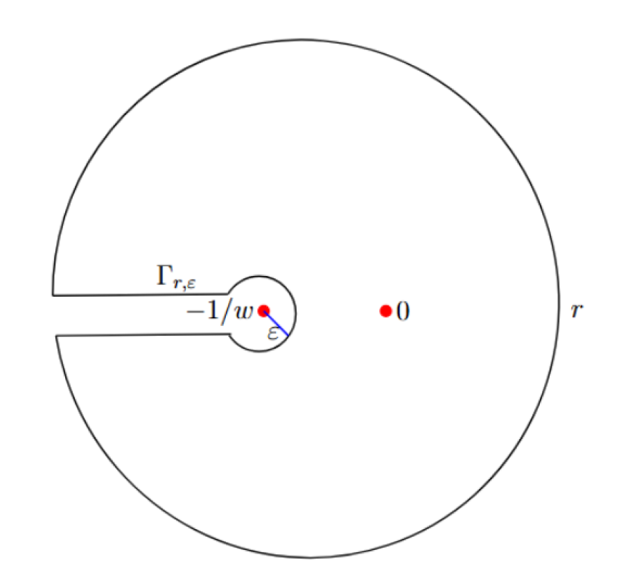
Figure 8: The last contour in the countour integral of (LABEL:cint12)

To make use of the above results, we proceed by Stokes theorem. Denote $\Gamma_{\varepsilon,r}$ to be the tubular neighborhood of height $\varepsilon$ of around the interval $[-r,-1/w-\varepsilon]$; see Figure 8.

Note that by (4.5), the LHS of (4.1) can be written as

$$\quad\lim_{r\rightarrow\infty}\int_{|z|<r}z^{j}\overline{\partial}\chi(z)\,dA(z)-\lim_{\varepsilon\rightarrow 0}\int_{\mathbb{D}(-1/w,\varepsilon)}z^{j}\overline{\partial}\chi(z)\,dA(z)-\lim_{\varepsilon\rightarrow 0}\int_{\Gamma_{\varepsilon,r}}z^{j}\overline{\partial}\chi(z)\,dA(z)$$

$$=\lim_{r\rightarrow\infty}\frac{1}{2i}\oint_{|z|=r}z^{j}\chi(z)\,dz-\lim_{\varepsilon\rightarrow 0}\frac{1}{2i}\oint_{\partial\mathbb{D}(-1/w,\varepsilon)}z^{j}\chi(z)\,dz-\lim_{\varepsilon\rightarrow 0}\frac{1}{2i}\oint_{\partial\Gamma_{\varepsilon,r}}z^{j}\chi(z)\,dz.$$

Recall from (4.4) and (4.6) that

$$\chi(z)=(z-w)^{NQ_{1}}\Big{(}\mathcal{A}_{1}(z)+\mathcal{B}_{1}(z)\Big{)}.$$

Moreover, using (4.7) and (4.8), along with the fact that $\mathcal{B}_{1}(z)$ is continuous away from $0$, it follows that

$$\lim_{r\rightarrow\infty}\oint_{|z|=r}z^{j}(z-w)^{NQ_{1}}\mathcal{B}_{1}(z)\,dz=0,$$

$$\lim_{\varepsilon\rightarrow 0}\oint_{\partial\mathbb{D}(-1/w,\varepsilon)}z^{j}(z-w)^{NQ_{1}}\mathcal{B}_{1}(z)\,dz=0,$$

$$\lim_{\varepsilon\rightarrow 0}\oint_{\partial\Gamma_{\varepsilon,r}}z^{j}(z-w)^{NQ_{1}}\mathcal{B}_{1}(z)\,dz=0.$$

Combining all of the above with (4.10), the LHS of (4.1) is given by

$$\begin{split}&\quad G_{k,N}\lim_{r\rightarrow\infty}\oint_{|z|=r}z^{j}(z-w)^{NQ_{1}}\Big{(}\frac{1}{1+wz}\Big{)}^{N+NQ_{0}-k}\Big{(}\frac{1}{z}\Big{)}^{k+1+NQ_{1}}\,dz\\ &-G_{k,N}\lim_{\varepsilon\rightarrow 0}\oint_{\partial\mathbb{D}(-1/w,\varepsilon)}z^{j}(z-w)^{NQ_{1}}\Big{(}\frac{1}{1+wz}\Big{)}^{N+NQ_{0}-k}\Big{(}\frac{1}{z}\Big{)}^{k+1+NQ_{1}}\,dz\\ &-G_{k,N}\lim_{\varepsilon\rightarrow 0}\oint_{\partial\Gamma_{\varepsilon,r}}z^{j}(z-w)^{NQ_{1}}\Big{(}\frac{1}{1+wz}\Big{)}^{N+NQ_{0}-k}\Big{(}\frac{1}{z}\Big{)}^{k+1+NQ_{1}}\,dz,\end{split}$$ (4.11)

where $G_{k,N}$ is given by (4.2).

The contour integral in (LABEL:cint12) does not depend on $r$ and $\varepsilon$ and the contour in

$$\oint_{|z|=r}-\oint_{\partial\Gamma_{\varepsilon,r}}-\oint_{\partial\mathbb{D}(-1/w,\varepsilon)}$$

is homotopic to a contour $\Gamma$ which has $0$ on the interior and $-1/w,\infty$ on the exterior (See Figure 8). Since the integrand is meromorphic we can deform the last contour in (LABEL:cint12) to $\Gamma$. This finishes the proof. ∎

4.1 Proof of Proposition 1.3

With Lemma 4.1 we are now ready to show that the planar orthogonal polynomials also satisfy non-Hermitian contour orthogonality.

Proof of Proposition 1.3.

If (1.28) holds true then from Lemma 4.1 we have for $\varepsilon<1/w$,

$$\oint_{|z|=\varepsilon}P_{n,N}(z)(z-w)^{NQ_{1}}\Big{(}\frac{1}{1+wz}\Big{)}^{N+NQ_{0}-k}\Big{(}\frac{1}{z}\Big{)}^{k+1+NQ_{1}}\,dz=0,$$ (4.12)

for $k=0,\dots n-1.$ Denote

$$Q_{n,N}(z):=z^{n}\,P_{n,N}(1/z).$$ (4.13)

Then changing variable $z\mapsto 1/z$ in (4.12) yields

$$\oint_{|z|=\varepsilon^{-1}}Q_{n,N}(z)(z+w)^{k}\frac{z^{N+NQ_{0}-n-1}(1-zw)^{NQ_{1}}}{(z+w)^{N+NQ_{0}}}dz=0,$$ (4.14)

for $k=0,\dots,n-1.$ Since $\{(z+w)^{k}\}_{k=0}^{n-1}$ also forms a basis for the space of holomorphic polynomials of degree at most $n-1$, we have

$$\oint_{|z|=\varepsilon^{-1}}Q_{n,N}(z)z^{k+1}\frac{z^{N+NQ_{0}-n-2}(1-zw)^{NQ_{1}}}{(z+w)^{N+NQ_{0}}}dz=0,$$ (4.15)

for $k=0,\dots,n-1.$

Rewriting (4.13) as $P_{n,N}(z)=Q_{n,N}(1/z)z^{n},$ we see by changing variables $z\mapsto\frac{1}{z}$ again in (4.15) and relabeling $k+1=n-j$ that

$$\oint_{|z|=\varepsilon}P_{n,N}(z)z^{j}(z-w)^{NQ_{1}}\Big{(}\frac{1}{1+wz}\Big{)}^{N+NQ_{0}}\Big{(}\frac{1}{z}\Big{)}^{n+NQ_{1}}\,dz=0,$$ (4.16)

for $j=0\dots n-1.$ By Cauchy’s theorem, the contour of integration (4.16) can be deformed to a contour $\Gamma$, as long as $0$ lies in the interior and $-1/w$ lies in the exterior of $\Gamma$. Hence $P_{n,N}$ is a family of orthogonal polynomials on the contour $\Gamma$ with respect to the weight (1.30). ∎

Remark 4.3.

We outline an alternative proof of Proposition 1.3, provided to us by Arno Kuijlaars (personal communication). Although the following proof is more elegant, we retain the previous proof since a similar argument will be used in the proof of Theorem 1.8. The statement (4.12) is equivalent to

$$\oint_{|z|=\varepsilon}P_{n,N}(z)(z-w)^{NQ_{1}}\Big{(}\frac{1}{1+wz}\Big{)}^{N+NQ_{0}}\Big{(}\frac{1}{z}\Big{)}^{n+NQ_{1}}(1+wz)^{k}z^{n-k-1}\,dz=0,$$ (4.17)

for $k=0,\dots,n-1$. As $k$ ranges from $0$ to $n-1$, we obtain a family of polynomials $\{p_{k}\}_{k=0}^{n-1}$ of degree $n-1$, where $p_{k}(z)=(1+wz)^{k}z^{n-k-1}$. If $w\neq 0$, this family is linearly independent. Consequently, $\{p_{k}\}_{k=0}^{n-1}$ forms a basis for the vector space of polynomials of degree less than $n$. Thus we can write the monomials $z^{j}$ with $0\leq j\leq n-1$ as a linear combination of $p_{k}$. This in turn implies (4.16).

5 Riemann-Hilbert analysis

By Proposition 1.3 the planar orthogonal polynomials $P_{n,N}$ satisfy non-Hermitian contour orthogonality, and consequently by the renowned work of [26] $P_{n,N}$ is a solution to the Riemann-Hilbert (RH) problem described below.

The RH problem is for the orthogonality contour $\Gamma$ (now fixed as given in Theorem 1.1). Namely, $\Gamma=\Gamma_{0}\cup\Gamma_{1}\cup\Gamma_{2}$, where $\Gamma_{0}$ is defined in Definition 3.6, and $\Gamma_{1}$ and $\Gamma_{2}$ are defined in Lemma 3.5.

RH problem 5.1.

$Y$ is the solution of the following RH problem.

• $Y:\mathbb{C}\setminus\Gamma\rightarrow\mathbb{C}^{2\times 2}$ where $\Gamma$ is a contour that encloses $0$ and has $-1/w$ on the exterior, with counterclockwise orientation.

• On $\Gamma$ we have

  $$Y_{+}(z)=Y_{-}(z)\begin{pmatrix}1&w_{n,N}(z)\\ 0&1\end{pmatrix},$$

  where $Y_{\pm}$ is the boundary values of $Y$ on $\Gamma$. Here, $w_{n,N}$ is given by (1.30).

• As $z\rightarrow\infty$ we have

  $$Y(z)=\left(I_{2}+\mathcal{O}(z^{-1})\right)\begin{pmatrix}z^{n}&0\\ 0&z^{-n}\end{pmatrix}.$$ (5.1)

Then we have $P_{n,N}(z)=Y_{1,1}(z)$.

5.1 Some preliminaries

At this point, one should observe from (1.26) and (1.30) that

$$w_{n,N}(z)=\frac{1}{z^{r_{0}}}e^{-N\mathcal{V}(z)},$$ (5.2)

where we also recall from the statement of Theorem 1.5 that $r_{0}=n-N$.

Definition 5.2.

We define

$$\varphi(z):=\int_{z_{1}}^{z}\sqrt{R_{0}(s)}\,ds,$$ (5.3)

where the contour of integration lies in $\mathbb{C}\setminus\left(\Gamma_{0}\cup\Gamma_{1}\cup[c_{0},\infty)\right)$. Then we also have from (3.3), (3.18) and (3.19) that $\tilde{\mathcal{U}}_{0}(z)=\operatorname{Re}\varphi(z)$.

Definition 5.3.

We define the $g$ function as

$$g(z):=\int\log(z-s)\,d\mu_{0}(s),$$ (5.4)

where the branch cut of the logarithm is taken in $\Gamma_{0}\cup\Gamma_{1}\cup[c_{0},\infty)$.

Notice that from (5.4) and (3.17), we have

$$g(z)=\log z+\mathcal{O}(z^{-1})\quad z\rightarrow\infty.$$ (5.5)

On the other hand, by (1.18) and (3.14), we have

$$\operatorname{Re}g(z)=-U^{\mu_{0}}(z),\qquad g^{\prime}(z)=C^{\mu_{0}}(z).$$

Then it follows from (3.21) that

$$2g^{\prime}(z)=\mathcal{V}^{\prime}(z)-\sqrt{R_{0}(z)}.$$

Here, the sign of $\sqrt{R_{0}(z)}$ can be identified by the $z\to\infty$ behaviour of both sides; cf. (1.24). Then by (1.25), we obtain

$$2g(z)=\mathcal{V}(z)-\varphi(z)+\ell_{0}$$ (5.6)

Recall that $\mathcal{U}_{0}$ is defined by (3.3). Then from item (2) of Theorem 1.1

$$\begin{split}w_{n,N}(z)e^{N\left(g_{+}(z)+g_{-}(z)-\ell_{0}\right)}&=z^{-r_{0}}e^{-N/2\left(\varphi_{+}(z)+\varphi_{-}(z)\right)}=\begin{cases}z^{-r_{0}},&z\in\Gamma_{0},\\ z^{-r_{0}}e^{-N\mathcal{U}_{0}(z)},&z\in\Gamma\setminus\Gamma_{0}.\end{cases}\end{split}$$ (5.7)

5.2 Transformation with the $g$ function

Our first transformation is the transformation with the $g$ function defined in (5.4). This normalizes the behaviour at infinity due to (5.5) and makes the $(1,2)$ entry of the jump on the contour $\Gamma_{0}$ to be $z^{-r_{0}}$ due to (5.7) while exponentially small on the rest of $\Gamma$.

Definition 5.4.

We define

$$X(z):=e^{-\frac{N}{2}\ell_{0}\sigma_{3}}Y(z)e^{-N\left(g(z)-\frac{\ell_{0}}{2}\right)\sigma_{3}}.$$ (5.8)

Here $\sigma_{3}=\begin{pmatrix}1&0\\ 0&-1\end{pmatrix}$, the third Pauli matrix. Then it follows from the RH problem 5.1, (5.7), and (5.5) that we have the following RH problem for $X$.

RH problem 5.5.

$X$ is the solution to the following RH problem.

• $X:\mathbb{C}\setminus\Gamma\rightarrow\mathbb{C}^{2\times 2}$ is analytic.

• $X_{+}=X_{-}J_{X}$ on $\Gamma$ with

  $$J_{X}:=\begin{cases}\begin{pmatrix}e^{-N\left(g_{-}(z)-g_{+}(z)\right)}&z^{-r_{0}}\\ 0&e^{N\left(g_{-}(z)-g_{+}(z)\right)}\end{pmatrix},\qquad&\mathrm{on}\hskip 5.69046pt\Gamma_{0},\vskip 3.0pt plus 1.0pt minus 1.0pt\\ \begin{pmatrix}1&z^{-r_{0}}e^{-N\mathcal{U}_{0}(z)}\\ 0&1\end{pmatrix},\qquad&\mathrm{on}\hskip 5.69046pt\Gamma\setminus\Gamma_{0}.\end{cases}$$ (5.9)

• As $z\rightarrow\infty$ we have

  $$X(z)=\left(I_{2}+\mathcal{O}(z^{-1})\right)\begin{pmatrix}z^{r_{0}}&0\\ 0&z^{-r_{0}}\end{pmatrix}.$$ (5.10)

5.3 Opening the lenses

The RH Problem 5.5 has oscillatory diagonal entries on the cut $\Gamma_{0}$. We open two lenses $L_{+},L_{-}$ on either side of $\Gamma_{0}$. The condition on the lens is that we must have $\operatorname{Re}\varphi(z)<0$ in the interior and the boundary of the lenses. This can be done in a neighborhood of $\Gamma_{0}$, as the measure $\mu_{0}$ has a strictly positive density on the interior.

Definition 5.6.

We define

$$T(z):=X(z)\begin{cases}I_{2},&z\in\mathbb{C}\setminus L_{\pm},\vskip 3.0pt plus 1.0pt minus 1.0pt\\ \begin{pmatrix}1&0\\ \mp z^{r_{0}}e^{N\varphi(z)}&1\end{pmatrix},&z\in L_{\pm}.\\ \end{cases}$$ (5.11)

RH problem 5.7.

$T$ satisfies the following RH problem.

• $T:\mathbb{C}\setminus\Sigma_{T}\rightarrow\mathbb{C}^{2\times 2}$ is analytic where $\Sigma_{T}=\Gamma\cup\partial L_{\pm}$.

• $T_{+}=T_{-}J_{T}$ on $\Sigma_{T}$ with

  $$J_{T}:=\begin{cases}\begin{pmatrix}0&z^{-r_{0}}\\ -z^{r_{0}}&0\end{pmatrix},\qquad&\mathrm{on}\hskip 5.69046pt\Gamma_{0},\vskip 3.0pt plus 1.0pt minus 1.0pt\\ \begin{pmatrix}1&z^{-r_{0}}e^{-N\mathcal{U}_{0}(z)}\\ 0&1\end{pmatrix},\qquad&\mathrm{on}\hskip 5.69046pt\Gamma\setminus\Gamma_{0},\vskip 3.0pt plus 1.0pt minus 1.0pt\\ \begin{pmatrix}1&0\\ z^{r_{0}}e^{N\varphi(z)}&1\end{pmatrix},\qquad&\mathrm{on}\hskip 5.69046pt\partial L_{\pm}.\end{cases}$$ (5.12)

• As $z\rightarrow\infty$, we have

  $$T(z)=\left(I_{2}+\mathcal{O}(z^{-1})\right)\begin{pmatrix}z^{r_{0}}&0\\ 0&z^{-r_{0}}\end{pmatrix}.$$ (5.13)

Since $r_{0}$ is fixed, observe that away from $z_{1}$ and $z_{2}$, the jumps on $\Gamma\setminus\Gamma_{0}$ and $\partial L_{\pm}$ converges to the identity matrix exponentially fast as $N\to\infty$. On the other hand, on $\Gamma_{0}$ it has simple jumps. This motivates the construction of the global matrix, which approximates $T(z)$ away from the branch points.

5.4 Global parametrix

RH problem 5.8.

We seek a matrix $M$ that satisfies the following conditions.

• $M:\mathbb{C}\setminus\Gamma\rightarrow\mathbb{C}^{2\times 2}$ is analytic.

• On $\Gamma_{0}$ we have $M_{+}(z)=M_{-}(z)J_{M}$, with

  $$J_{M}:=\begin{pmatrix}0&z^{-r_{0}}\\ -z^{r_{0}}&0\end{pmatrix}.$$ (5.14)

• As $z\rightarrow x^{*}$, with $x^{*}\in\{z_{1},z_{2}\}$, we have

  $$M(z)=\mathcal{O}((z-x^{*})^{1/4}).$$

• As $z\rightarrow\infty$ we have

  $$M(z)=\left(I_{2}+\mathcal{O}(z^{-1})\right)\begin{pmatrix}z^{r_{0}}&0\\ 0&z^{-r_{0}}\end{pmatrix}.$$ (5.15)

Lemma 5.9.

Define

$$D(z):=\sqrt{\frac{\rho}{a}}\frac{1}{F_{1}(z)},$$ (5.16)

where $F_{1}$, one of the inverses of the map $f$, is given by (2.6). Then it satisfies the following.

• $D(z)$ is analytic and nonzero in $\mathbb{C}\setminus\Gamma_{0}$;

• $D_{+}(z)D_{-}(z)=z$ if $z\in\Gamma_{0}$;

• $D(z)=D_{\infty}z+\mathcal{O}(1)$ as $z\rightarrow\infty$, where $D_{\infty}:=\frac{1}{\sqrt{\rho a}}.$

Proof.

Item (1) is immediate from definition (5.16). Item (3) follows from (2.4). We prove item (2). By direct computation using (1.21) and (2.3), we have

$$f(u)=\frac{\rho}{a}\frac{1}{\mathrm{deck}(u)u}$$ (5.17)

Notice that by (2.5), we have

$$F_{1}(z_{\pm})=F_{2}(z_{\mp})=\mathrm{deck}(F_{1}(z_{\mp})),\quad z\in\Gamma_{0}.$$

Thus we obtain

$$D_{+}(z)D_{-}(z)=\frac{\rho}{a}\frac{1}{F_{1}(z)}\frac{1}{\mathrm{deck}(F_{1}(z))}=z,\quad z\in\Gamma_{0}.$$ (5.18)

∎

Next, we consider

$$M(z)=D_{\infty}^{-r_{0}\sigma_{3}}N(z)D(z)^{r_{0}\sigma_{3}},$$ (5.19)

and the Riemann-Hilbert problem associated with $N(z)$.

RH problem 5.10.

Following RH problem 5.8 and (5.19), we seek a matrix $N$ that satisfies the following conditions.

• $N:\mathbb{C}\setminus\Gamma\rightarrow\mathbb{C}^{2\times 2}$ is analytic.

• On $\Gamma_{0}$ we have $N_{+}(z)=N_{-}(z)J_{N}$, with

  $$J_{N}:=\begin{pmatrix}0&1\\ -1&0\end{pmatrix}.$$ (5.20)

• As $z\rightarrow x^{*}$, with $x^{*}\in\{z_{1},z_{2}\}$, we have

  $$N(z)=\mathcal{O}((z-x^{*})^{1/4}).$$

• As $z\rightarrow\infty$ we have

  $$N(z)=\left(I_{2}+\mathcal{O}(z^{-1})\right).$$ (5.21)

We construct the solution of RH Problem 5.10 by means of the conformal map $F_{1}$ defined in (2.6). Denote

$$\tilde{\Gamma}_{\pm}:=F_{1}(\Gamma_{0\pm})=F_{2}(\Gamma_{0\mp}).$$

We are looking for a solution of the form

$$N(z)=\begin{pmatrix}N_{1}(F_{1}(z))&N_{1}(F_{2}(z))\\ N_{2}(F_{1}(z))&N_{1}(F_{2}(z))\end{pmatrix},$$ (5.22)

where $N_{1}$ and $N_{2}$ are two scalar-valued functions on $\mathbb{C}\setminus\tilde{\Gamma}_{\pm}$.

In order to satisfy the jump condition (5.20) we must have

$$N_{k_{+}}(u)=\begin{cases}-N_{k_{-}}(u),&u\in\tilde{\Gamma}_{+},\\ N_{k_{-}}(u),&u\in\tilde{\Gamma}_{-}.\end{cases}$$ (5.23)

Hence $N_{k}$ is analytic across $\tilde{\Gamma}_{-}$. We recall from (2.4) that as $z\rightarrow\infty$

$$F_{1}(z)=\frac{\rho}{z}+\mathcal{O}(z^{-2}),\qquad F_{2}(z)=\frac{1}{a}+\mathcal{O}(z^{-1}),$$ (5.24)

and a direct computation shows in (1.21)

$$\frac{1}{\sqrt{f^{\prime}(z)}}=(z-1/a)\frac{i}{\sqrt{a(b-a)\rho}}+\mathcal{O}((z-1/a)^{2}),\quad z\rightarrow 1/a,$$ (5.25)

$$\frac{1}{\sqrt{f^{\prime}(z)}}=iz\frac{1}{\sqrt{\rho}}+\mathcal{O}(z),\quad z\rightarrow 0.$$ (5.26)

With this in mind, we set

$$N_{1}(u):=a_{1}\frac{1}{\sqrt{f^{\prime}(u)}}\frac{1}{u},\qquad N_{2}(u):=a_{2}\frac{1}{\sqrt{f^{\prime}(u)}}\frac{1}{u-1/a},$$ (5.27)

where

$$a_{1}=i\sqrt{\rho},\qquad a_{2}=-i\sqrt{\frac{a}{b-a}\frac{1}{\rho}},$$ (5.28)

and the branch of the square root of $\sqrt{f^{\prime}(u)}$ is taken on $\tilde{\Gamma}_{+}$.

Since $f(F_{j}(z))=z$ $(j=1,2)$ we have the chain rule

$$\frac{1}{\sqrt{f^{\prime}(F_{j}(z))}}=\sqrt{F_{j}^{\prime}(z)}.$$

Then by (5.22) and (5.27), we have

$$N(z)=\begin{pmatrix}a_{1}\frac{\sqrt{F_{1}^{\prime}(z)}}{F_{1}(z)}&a_{1}\frac{\sqrt{F_{2}^{\prime}(z)}}{F_{2}(z)}\\ a_{2}\frac{\sqrt{F_{1}^{\prime}(z)}}{F_{1}(z)-1/a}&a_{2}\frac{\sqrt{F_{2}^{\prime}(z)}}{F_{2}(z)-1/a}\end{pmatrix}.$$ (5.29)

As a consequence, by (5.19), we obtain

$$M(z)=D_{\infty}^{-r_{0}\sigma_{3}}\begin{pmatrix}a_{1}\frac{\sqrt{F_{1}^{\prime}(z)}}{F_{1}(z)}&a_{1}\frac{\sqrt{F_{2}^{\prime}(z)}}{F_{2}(z)}\\ a_{2}\frac{\sqrt{F_{1}^{\prime}(z)}}{F_{1}(z)-1/a}&a_{2}\frac{\sqrt{F_{2}^{\prime}(z)}}{F_{2}(z)-1/a}\end{pmatrix}D(z)^{r_{0}\sigma_{3}}.$$ (5.30)

5.5 Local parametrices

Local parametrices are defined in a neighbourhood of the branch points $z_{j}$ and are constructed in the discs $\mathbb{D}(z_{j},\delta)$ for $j\in\{1,2\}$. We take

$$D=\mathbb{D}(z_{1},\delta)\cup\mathbb{D}(z_{2},\delta).$$ (5.31)

For $\delta>0$ small, the local parametrices are defined in $D$, with jump matrices that agree with $J_{T}$ given in (5.12). In addition, it agrees with $M$ on the boundary of the discs up to an error $\mathcal{O}(n^{-1})$ as $n\rightarrow\infty$. Specifically, we introduce $P(z)$ according to the following RH problem.

RH problem 5.11.

$P$ satisfies the following RH problem.

• $P(z)$ analytic in $D\setminus\Sigma_{P}$ where $\Sigma_{P}:=\Sigma_{T}\cap D$. (Recall $\Sigma_{T}$ in RH problem 5.7.)

• $P_{+}=P_{-}J_{P}$ on $\Sigma_{P}$ with

  $$J_{P}:=\begin{cases}\begin{pmatrix}0&z^{-r_{0}}\\ -z^{r_{0}}&0\end{pmatrix},&\quad\mathrm{on}\hskip 5.69046pt\Gamma_{0}\cap D,\vskip 3.0pt plus 1.0pt minus 1.0pt\\ \begin{pmatrix}1&z^{-r_{0}}e^{-N\mathcal{U}_{0}(z)}\\ 0&1\end{pmatrix},&\quad\mathrm{on}\hskip 5.69046pt\Gamma\setminus\Gamma_{0}\cap D,\vskip 3.0pt plus 1.0pt minus 1.0pt\\ \begin{pmatrix}1&0\\ z^{r_{0}}e^{N\varphi(z)}&1\end{pmatrix},&\quad\mathrm{on}\hskip 5.69046pt\partial L_{\pm}\cap D.\end{cases}$$ (5.32)

• $P(z)$ matches with the outer parametrix $M$ that is

  $$P(z)=M(z)\left(1+\mathcal{O}(n^{-1})\right)\quad n\rightarrow\infty,$$ (5.33)

  uniformly as $z\in\partial D$.

The functions $\varphi(z)=\mathrm{const}\times(z-z_{j})^{3/2}\left(1+\mathcal{O}(z-z_{j})^{1/2}\right)$ and the local parametrices of $z^{(r_{0}/2)\sigma_{3}}P(z)z^{(-r_{0}/2)\sigma_{3}}$ can be constructed out of Airy functions; see for instance [22]. We omit the construction here, as the precise form is not necessary for our main purpose.

5.6 Final transformation

Definition 5.12.

We make the final transformation

$$S(z):=\begin{cases}T(z)M(z)^{-1},&\quad z\in\mathbb{C}\setminus\left(D\cup\partial L_{\pm}\cup\Gamma\right)\vskip 3.0pt plus 1.0pt minus 1.0pt\\ T(z)P(z)^{-1},&\quad z\in D\setminus(\partial L_{\pm}\cup\Gamma).\end{cases}$$ (5.34)

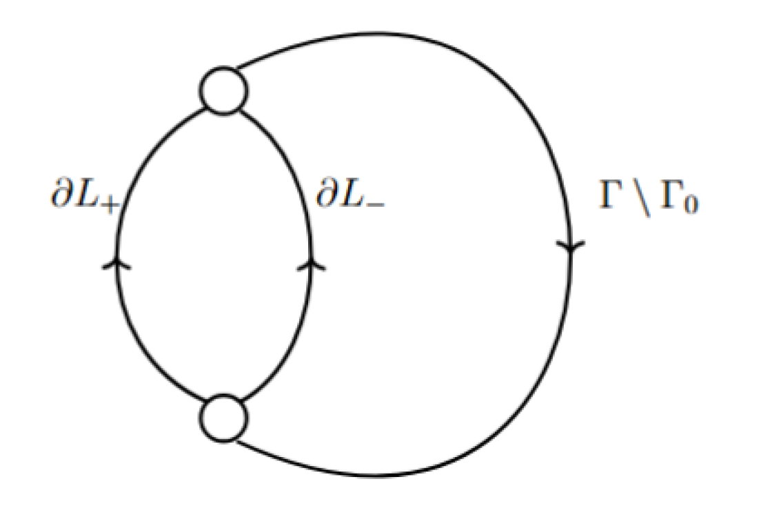
Figure 9: The jump contour $\Sigma_{S}$

The jump matrices of $T$ and $M$ coincide on $\Gamma_{0}$, while the jump matrices of $T$ and $P$ coincide on $D$. It follows that $S(z)$ has an analytic continuation to $\mathbb{C}\setminus\Sigma_{S}$, as shown in Figure 9. The matching condition (5.33) ensures that $PM^{-1}=I_{2}+\mathcal{O}(N^{-1})$ uniformly as $N\to\infty$ on $\partial D$. Thus, as $N\to\infty$,

$$S_{+}(z)=S_{-}(z)\left(I+\mathcal{O}(N^{-1})\right),$$ (5.35)

uniformly on $\partial D$. While on the rest of the contour $\Sigma_{S}$, as $N\to\infty$, there exists $c>0$ such that

$$S_{+}(z)=S_{-}(z)\left(I+\mathcal{O}(e^{-cN})\right),$$ (5.36)

uniformly on $\partial D$. Since $S(z)\rightarrow I_{2}$ as $z\to\infty$, standard arguments yield that as $N\to\infty,$

$$S(z)=I+\mathcal{O}\Big{(}\frac{1}{N(1+|z|)}\Big{)},$$ (5.37)

uniformly in $z\in\mathbb{C}\setminus\Sigma_{S}$.

5.6.1 Proof of Theorem 1.5

Proof.

We take $z$ in a compact subset $K$ of $\overline{\mathbb{C}}\setminus\Gamma_{0}$. We may further assume that $L_{\pm}$ and $\mathbb{D}(z_{j},\delta)$ are such that $K$ is in their exterior.

Following the transformation

$$Y\mapsto X\mapsto T\mapsto S$$

and recalling $P_{n,N}=Y_{1,1}$ we obtain the asymptotic formula

$$P_{n,N}(z)=e^{Ng(z)}M_{1,1}(z)(1+\mathcal{O}(N^{-1})),\quad z\in\mathbb{C}\setminus\left(D\cup L_{\pm}\right),$$ (5.38)

where the convergence is uniform in $K$. By computing the $(1,1)$-entry of the matrix $M$ given in (5.30), we obtain (1.32). ∎

5.6.2 Proof of Theorem 1.7

Proof.

The proof is immediate from the strong asymptotic formula (1.32). By (5.27), we have $M_{1,1}(z)\neq 0$ for $z\in\mathbb{C}\setminus\Gamma_{0}$. Hence, the zeros of $P_{n,N}$ accumulate on $\Gamma_{0}$ as $N\rightarrow\infty$.

From (1.32) we further conclude that

$$\lim_{n\rightarrow\infty}\frac{1}{n}\log|P_{n,N}(z)|=\operatorname{Re}g(z)=\int\log|z-s|\,d\mu_{0}(s),$$ (5.39)

uniformly for compact subsets of $\mathbb{C}\setminus\Gamma_{0}$. It is well known [47] that this implies $\mu_{0}$ is the weak limit of the normalized zero counting measure; see also [35]. ∎

6 Proof of Theorem 1.8

Recall $\ell_{\mathrm{2D}}$ in (1.20). We first relate the constants $\ell_{\mathrm{2D}}$ and $\ell_{0}$ appearing in Theorem 1.1

Lemma 6.1.

We have the following relation between $\ell_{\mathrm{2D}}$ and $\ell_{0}$:

$$\ell_{0}=\ell_{\mathrm{2D}} +(1+Q_{0})\log w+\operatorname{Re}g(0)$$ (6.1)

$$\quad-(1+Q_{1})\log(1+Q_{1})-Q_{0}\log Q_{0}+(1+Q_{0}+Q_{1})\log\left(1+Q_{0}+Q_{1}\right).$$

Proof.

Recall that $\tilde{\mathcal{U}}_{0}$ is given in (3.19). We observe as $z\rightarrow 0$ we have

$$2\tilde{\mathcal{U}}_{0}(z)=2(1+Q_{1}+Q_{0}) \log\Big{(}1+\frac{b\rho^{2}}{a}\Big{)}+\tilde{\mathcal{U}}(z)+\tilde{\mathcal{U}}(s)$$ (6.2)

$$-(1+Q_{1}+Q_{0})\log(1+s^{2})+\mathcal{O}(z),$$

where $s=\frac{b\rho^{2}}{az}$. This identity follows from the steps of Proposition 3.3, replacing $c_{0}$ by $0$ and noting $F_{1}(0)=1/b$ since $f(1/b)=0$ follows from the definition (1.21), and that $\mathrm{deck}(1/b)=\infty$ by (2.3). Then using the expansion

$$f\Big{(}\frac{1}{\mathrm{deck}(F_{1}(z))}\Big{)}=\frac{b\rho^{2}}{az}+\mathcal{O}(1),\quad z\rightarrow 0,$$

gives (6.2).

By (3.19), (3.3) and (3.21), the LHS of (6.2) can be written as

$$2\tilde{\mathcal{U}}_{0}(z)=4U^{\mu_{0}}(z)+2(1+Q_{1})\log|z|+2(1+Q_{0})\log|z+1/w|-2Q_{1}\log|z-w|+2\ell_{0}.$$

Then by (5.4), we have

$$2\tilde{\mathcal{U}}_{0}(z)=2(1+Q_{1})\log|z|-2(1+Q_{0})\log w-2Q_{1}\log w-4\operatorname{Re}g(0)+2\ell_{0}+\mathcal{O}(z),$$ (6.3)

as $z\to 0$.

Next, we compute the asymptotic behaviour of the RHS of (6.2) as $z\to 0$. By (3.2) we can write

$$\tilde{\mathcal{U}}(z)=2U^{\mu_{0}}(z)-2Q_{1}\log|z-w|+(1+Q_{0}+Q_{1})\log(1+|z|^{2})+\ell_{2D}.$$

Therefore, we have

$$\tilde{\mathcal{U}}(z)=-2Q_{1}\log w-2\operatorname{Re}g(0)+\ell_{2D}+\mathcal{O}(z),$$ (6.4)

as $z\to 0$. On the other hand, we have

$$\tilde{\mathcal{U}}(s)=2Q_{0}\log|s|+\ell_{\mathrm{2D}}+\mathcal{O}(1/s),$$ (6.5)

as $s\to\infty$. Hence combining (6.4) and (6.5) we find that the RHS of (6.2) has an expansion

$$-2Q_{1}\log w-2\operatorname{Re}g(0) +2\ell_{\mathrm{2D}}+2(1+Q_{1})\log|z|-2(1+Q_{1})\log\frac{b\rho^{2}}{a}$$ (6.6)

$$+2(1+Q_{0}+Q_{1})\log\Big{(}1+\frac{b\rho^{2}}{a}\Big{)}+\mathcal{O}(z),$$

as $z\to 0$. Now substituting [14, Eq 2.60],

$$\frac{b\rho^{2}}{a}=\frac{1+Q_{1}}{Q_{0}},$$ (6.7)

equating (6.3) with (6.6) gives (6.1). ∎

Recall that $h_{n}\equiv h_{n,N}$ is the squared norm in the planar orthogonality (1.13). We also denote by $\tilde{h}_{n}\equiv\tilde{h}_{n,N}$ the squared norm in the non-Hermitian contour orthogonality (1.29), i.e.

$$\oint_{\Gamma}P_{n,N}^{2}(z)\frac{(z-w)^{NQ_{1}}}{(1+zw)^{N+NQ_{0}}}\frac{1}{z^{n+NQ_{1}}}=\tilde{h}_{n,N}.$$ (6.8)

Lemma 6.2.

We have

$$\tilde{h}_{n,N}=-\frac{1}{G_{n,N}}P_{n+1,N}(0)\,h_{n,N},$$ (6.9)

where $G_{n,N}$ is defined by (4.2).

Proof.

The proof follows the same approach as in [4, Appendix E]. We define

$$\mu_{ij}:=\int_{\mathbb{C}}z^{i}\,\overline{z}^{j}\,\frac{|z-w|^{NQ_{1}}}{(1+|z|^{2})^{N(1+Q_{0}+Q_{1})}}\,dA(z)$$ (6.10)

and

$$\nu_{i}:=\int_{\Gamma}z^{i}(z-w)^{NQ_{1}}\frac{1}{(1+zw)^{N+NQ_{0}}}\frac{1}{z^{n+NQ_{1}}}\,dz.$$ (6.11)

Then from the the determinantal expressions for $P_{n,N}$, we have

$$h_{n}=\frac{\det[\mu_{ij}]_{0\leq i,j\leq n}}{\det[\mu_{ij}]_{0\leq i,j\leq n-1}},\qquad\tilde{h}_{n}=\frac{\det[\nu_{i+j}]_{0\leq i,j\leq n}}{\det[\nu_{i+j}]_{0\leq i,j\leq n-1}}.$$ (6.12)

We relate first relate $\det[\nu_{i+j}]_{0\leq i,j\leq n}$ to $\det[\mu_{ij}]_{0\leq i,j\leq n}$. Observe that, with the change of variables $z\mapsto 1/z$ and the relabelling $k=n+1-j$, we have

$$\quad\det[\nu_{i+j}]_{0\leq i,j\leq n}=\det\bigg{[}\int_{\Gamma}z^{i+1}z^{j}\frac{(z-w)^{NQ_{1}}}{(1+zw)^{N+NQ_{0}}}\frac{1}{z^{n+NQ_{1}+1}}\,dz\bigg{]}_{0\leq i,j\leq n}$$

$$=(-1)^{n(n+1)/2}\det\bigg{[}\int_{\Gamma^{-1}}\frac{z^{k+1}}{z^{i+1}}\frac{(1-zw)^{NQ_{1}}}{(z+w)^{N+NQ_{0}}}z^{N+NQ_{0}-2}dz\bigg{]}_{0\leq i,k\leq n}$$

$$=(-1)^{n(n+1)/2}\det\left[\int_{\Gamma^{-1}}\frac{z(z+w)^{k}}{z^{i+1}}\frac{(1-zw)^{NQ_{1}}}{(z+w)^{N+NQ_{0}}}z^{N+NQ_{0}-2}dz\right]_{0\leq i,k\leq n}$$

$$=(-1)^{n(n+1)/2}\det\bigg{[}\int_{\Gamma}z^{i+1}(z-w)^{NQ_{1}}\frac{1}{(1+zw)^{N+NQ_{0}-k}}\frac{1}{z^{NQ_{1}+1+k}}\,dz\bigg{]}_{0\leq i,k\leq n},$$

where we have used (1.29). Then it follows from Lemma 4.1 that $\det[\nu_{i+j}]_{0\leq i,j\leq n}$ is given by

$$\quad(-1)^{n(n+1)/2}\prod_{\ell=0}^{n}\frac{1}{G_{\ell,N}}\det\bigg{[}\int_{\mathbb{C}}z^{i+1}\overline{(z-w)}^{k}\frac{|z-w|^{NQ_{1}}}{(1+|z|^{2})^{N(1+Q_{0}+Q_{1})+1}}dA(z)\bigg{]}_{0\leq i,k\leq n}$$ (6.13)

$$=(-1)^{n(n+1)/2}\prod_{\ell=0}^{n}\frac{1}{G_{\ell,N}}\det[\mu_{ik}]_{\begin{subarray}{c}1\leq i\leq n+1\\ 0\leq k\leq n\end{subarray}}$$

$$=(-1)^{n(n+1)/2}\prod_{\ell=0}^{n}\frac{1}{G_{\ell,N}}(-1)^{n+1}P_{n+1,N}(0)\det[\mu_{ik}]_{0\leq i,k\leq n}.$$

Similarly, we have

$$\det[\nu_{i+j}]_{0\leq i,j\leq n-1}=(-1)^{n(n-1)/2}\prod_{\ell=0}^{n-1}\frac{1}{G_{\ell,N}}\det[\mu_{ik}]_{0\leq i,k\leq n-1}.$$ (6.14)

Combining these, we obtain the desired result (6.9). ∎

We are now ready to prove Theorem 1.8.

Proof of Theorem 1.8.

Define

$$\hat{h}_{n}:=\tilde{h}_{n}w^{N+NQ_{0}}.$$ (6.15)

The large $n$ asymptotic for $\hat{h}_{n}$ can be written in terms of solution of the RH problem 5.1. In particular it follows from the standard theory [22] that

$$\hat{h}_{n}=-2\pi i \lim_{z\rightarrow\infty}z^{n+1}\bigg{[}e^{N\frac{\ell_{0}}{2}\sigma_{3}}\bigg{(}I_{2}+\mathcal{O}\Big{(}\frac{1}{N(1+|z|)}\Big{)}\bigg{)}M(z)e^{N(g(z)-\frac{\ell_{0}}{2})\sigma_{3}}\bigg{]}_{12}$$ (6.16)

$$=2\pi i(\rho a)^{r_{0}}\sqrt{a(b-a)}\rho e^{N\ell_{0}}\left(1+\mathcal{O}(N^{-1})\right).$$

Here, in the second line, we have used

$$N_{1,2}(z)=i\frac{\sqrt{\rho F_{2}^{\prime}(z)}}{F_{2}(z)}=-\rho\frac{\sqrt{a(b-a)}}{z}+\mathcal{O}(z^{-1}),\qquad z\rightarrow\infty,$$ (6.17)

which follows from RH problem 5.8.

By (2.6), we also have

$$i\frac{\sqrt{\rho F_{1}^{\prime}(z)}}{F_{1}(z)}=-\sqrt{\frac{b-a}{b}}+\mathcal{O}(z)\qquad z\rightarrow 0.$$ (6.18)

Then from (1.32) we obtain,

$$P_{n+1,N}(0)=-\left(\rho b\right)^{r_{0}+1}\sqrt{\frac{b-a}{b}}e^{Ng(0)}\left(1+\mathcal{O}(N^{-1})\right).$$ (6.19)

Combining (6.9), (6.15), (6.16) and (6.19) we obtain

$$h_{n,N}=2\pi i\,G_{n,N}\left(\frac{a}{b}\right)^{r_{0}}\sqrt{\frac{a}{b}}e^{N\ell_{0}}e^{-Ng(0)}\frac{1}{w^{N+NQ_{0}}}\left(1+\mathcal{O}(N^{-1})\right)$$ (6.20)

Notice here that by (4.2) and Stirling approximation

$$\Gamma(z)=\sqrt{\frac{2\pi}{z}}z^{z}e^{-z}\left(1+\mathcal{O}(z^{-1}\right),$$ (6.21)

we have

$$2iG_{n,N}=\sqrt{\frac{2\pi}{N}} e^{N\left(Q_{0}\log Q_{0}+(1+Q_{1})\log(1+Q_{1})-(1+Q_{0}+Q_{1})\log(1+Q_{0}+Q_{1})\right)}$$ (6.22)

$$\times\Big{(}\frac{1+Q_{1}}{Q_{0}}\Big{)}^{1+r_{0}}\sqrt{\frac{Q_{0}}{(Q_{0}+Q_{1}+1)(Q_{1}+1)}}\left(1+\mathcal{O}(N^{-1})\right).$$

Substituting $G_{n,N}$ and replacing $\ell_{0}$ by $\ell_{\mathrm{2D}}$ as given in Lemma 6.1 in (6.9) we obtain

$$h_{N}=\pi\sqrt{\frac{2\pi}{N}}\Big{(}\frac{1+Q_{1}}{Q_{0}}\Big{)}^{1+r_{0}}\sqrt{\frac{Q_{0}}{(Q_{0}+Q_{1}+1)(Q_{1}+1)}}\Big{(}\frac{a}{b}\Big{)}^{r_{0}+1/2}e^{N\ell_{\mathrm{2D}}}\left(1+\mathcal{O}(N^{-1})\right).$$

Then by (6.7), we obtain (1.35). This finishes the proof of Theorem 1.8. ∎

Acknowledgements

We are grateful to Arno Kuijlaars for his insights and comments. Sung-Soo Byun was supported by the New Faculty Startup Fund at Seoul National University and by the National Research Foundation of Korea grant (RS-2023-00301976, RS-2025-00516909). Funding support to Peter Forrester for this research was through the Australian Research Council Discovery Project grant DP250102552. Sampad Lahiry acknowledges financial support from the International Research Training Group (IRTG) between KU Leuven and University of Melbourne and Melbourne Research Scholarship of University of Melbourne.

Appendix A Appendix

The measure $\mu_{0}$ obtained in Theorem 1.1 can also be characterized as a solution of an equilibrium problem. An alternate approach is to start with the equilibrium problem and build the algebraic curve from the measure. We sketch the steps here.

Consider the following max-min problem

$$\max_{\Gamma\in\mathcal{F}}\min_{\begin{subarray}{c}{\mathrm{supp}\hskip 2.84544pt\mu\subset\Gamma}\\ \mu(\mathbb{C})=1\end{subarray}}\bigg{[}\iint\log\frac{1}{|x-y|}\,d\mu(x)\,d\mu(y)+\int\operatorname{Re}\mathcal{V}(x)\,d\mu(x)\bigg{]},$$ (A.1)

where the maximum is taken over $\mathcal{F}$ the collection of all closed contours $\mathcal{F}$ which has $0$ in the interior and $-1/w$ in the exterior, and the minimum is taken over the set of Borel probability measures $\mu$ on $\Gamma$. By standard capacity estimates we have been able to show that the solution to the max-min problem exists and is unique and the max-min contour $\Gamma_{0}$ is a critical set in the following sense.

Fix a contour $F_{0}$ in $\mathcal{F}$, then denote

$$I^{\mathcal{V}}(F_{0}):=\min_{\begin{subarray}{c}{\mathrm{supp}\hskip 2.84544pt\mu\subset F_{0}}\\ \mu(\mathbb{C})=1\end{subarray}}\bigg{[}\iint\log\frac{1}{|x-y|}\,d\mu(x)\,d\mu(y)+\int\operatorname{Re}\mathcal{V}(x)\,d\mu(x)\bigg{]}.$$ (A.2)

The solution to the equilibrium problem exists and is unique as the external field is admissible.

Next consider any $C_{c}^{2}$ function $h(z):\mathbb{C}\rightarrow\mathbb{C}$ and its one-parameter deformation

$$F_{0}^{t}:=\{z+th(z)\hskip 2.84544pt|\hskip 2.84544ptz\in F_{0}\}.$$ (A.3)

Here $t$ is chosen small enough such that $F_{0}^{t}\in\mathcal{F}$. Then the set $F_{0}$ is a critical set, if we have

$$\lim_{t\rightarrow 0}\frac{I^{\mathcal{V}}(F_{0}^{t})-I^{\mathcal{V}}(F_{0})}{t}=0,\quad t\in\mathbb{R}.$$ (A.4)

Having defined the notion of critical set we turn to the notion of critical measure.

For a Borel probability measure, denote

$$I_{\mathcal{V}}(\mu)=I(\mu)+\int\operatorname{Re}\mathcal{V}(z)d\mu(z).$$ (A.5)

We now define the Schiffer variations: For a $C^{2}$ compactly supported test function $h$ in $\mathbb{C}$, denote

$$h_{t}(z)=z+th(z).$$ (A.6)

Then we consider the $h_{t}$ perturbation of the measure by $\mu\rightarrow\mu_{t,h}$ induced by the push-forward perturbation $h_{t}$, defined in the weak sense as

$$\int fd\mu_{t,h}=\int f(x+th(x))d\mu(x).$$ (A.7)

The critical measure is such that for all $C_{c}^{2}$ test function $h$ we have

$$\lim_{t\rightarrow 0}\frac{I_{\mathcal{V}}(\mu)-I_{\mathcal{V}}(\mu_{t,h})}{t}=0.$$ (A.8)

It is well known [37] that for log rational external fields, for the critical measure which we denote now by $\mu_{0}$ there exists a rational function $R(z)$ such that

$$\Big{(}C^{\mu_{0}}(z)-\frac{\mathcal{V}^{\prime}(z)}{2}\Big{)}^{2}=R(z).$$ (A.9)

Now to relate the critical set and critical measure, one uses a well-known result [37, 46] that the equilibrium measure of the critical set is a critical measure.

Hence obtaining $\mu_{0}$ in this fashion, one can define the spherical Schwarz function as (3.12) and due to (A.9), $S_{1},S_{2}$ are branches of a meromorphic function and the spectral curve $P(S,z)$ in (2.21) is then obtained. To obtain the droplet, one can then verify that the parametrization

$$\Big{(}\frac{f(1/w)}{1+f(w)f(1/w)},f(w)\Big{)}$$

is a rational parametrization of $P(S,z)=0$.

References

- [1] Y. Ameur, H. Hedenmalm and N. Makarov, Fluctuations of eigenvalues of random normal matrices, Duke Math. J. 159 (2011), 31–81.
- [2] Y. Ameur, H. Hedenmalm and N. Makarov, Random normal matrices and Ward identities, Ann. Probab. 43 (2015), 1157–1201.
- [3] Y. Ameur, N-G. Kang and S.-M. Seo, The random normal matrix model: insertion of a point charge, Potential Anal. 58 (2023), 331–372.
- [4] F. Balogh, M. Bertola, S.-Y. Lee and K.D.T.-R. McLaughlin, Strong asymptotics of the orthogonal polynomials with respect to a measure supported on the plane, Comm. Pure Appl. Math. 68 (2015), 112–172.
- [5] F. Balogh, T. Grava and D. Merzi, Orthogonal polynomials for a class of measures with discrete rotational symmetries in the complex plane, Constr. Approx. 46 (2017), 109–169.
- [6] S. Berezin, A.B.J. Kuijlaars, and I. Parra, Planar orthogonal polynomials as type I multiple orthogonal polynomials, SIGMA 19 (2023), Paper No. 020, 18pp.
- [7] M. Bertola, J. G. Elias Rebelo and T. Grava, Painlevé IV critical asymptotics for orthogonal polynomials in the complex plane, SIGMA Symmetry Integrability Geom. Methods Appl. 14 (2018), Paper No. 091, 34pp.
- [8] P.M. Bleher and A.B.J Kuijlaars, Orthogonal polynomials in the normal matrix model with a cubic potential, Adv. Math. 230 (2012), 1272–1321.
- [9] R. Bøgvad and B. Shapiro, On mother body measures with algebraic Cauchy transform, Enseign. Math. 62 (2016), 117–142.
- [10] J.S. Brauchart, P.D. Dragnev, E.B. Saff and R.S. Womersley, Logarithmic and Riesz equilibrium for multiple sources on the sphere: the exceptional case, Contemporary Computational Mathematics - A Celebration of the 80th Birthday of Ian Sloan (J. Dick, F. Kuo, and H. Woźniakowski, eds.), Springer, Cham, 2018, pp. 179–203.
- [11] S.-S. Byun, Planar equilibrium measure problem in the quadratic fields with a point charge, Comput. Methods Funct. Theory 24 (2024), 303–332.
- [12] S.-S. Byun, C. Charlier, P. Moreillon and N. Simm, Planar equilibrium measure for the truncated ensembles with a point charge, manuscript in progress.
- [13] S.-S. Byun and P.J. Forrester, Progress on the study of the Ginibre ensembles, KIAS Springer Series in Mathematics 3, Springer, 2025.
- [14] S.-S. Byun, P.J. Forrester and S. Lahiry, Properties of the one-component Coulomb gas on a sphere with two macroscopic external charges, arXiv:2501.05061.
- [15] S.-S. Byun, N.-G. Kang and S.-M. Seo, Partition functions of determinantal and Pfaffian Coulomb gases with radially symmetric potentials, Comm. Math. Phys. 401 (2023), 1627–1663.
- [16] S.-S Byun, S.-M. Seo and M. Yang, Free energy expansions of a conditional GinUE and large deviations of the smallest eigenvalue of the LUE, arXiv:2402.18983.
- [17] S.-S Byun, N.-G. Kang, S.-M. Seo and M. Yang, Free energy of spherical Coulomb gases with point charges, arXiv:2501.07284.
- [18] S.-S. Byun and M. Yang, Determinantal Coulomb gas ensembles with a class of discrete rotational symmetric potentials, SIAM J. Math. Anal. 55 (2023), 6867–6897.
- [19] S.-S. Byun and E. Yoo, Three topological phases of the elliptic Ginibre ensembles with a point charge, arXiv:2502.02948.
- [20] J.G. Criado del Rey and A.B.J. Kuijlaars, An equilibrium problem on the sphere with two equal charges, preprint arXiv:1907.0480.
- [21] J.G. Criado del Rey and A.B.J. Kuijlaars, A vector equilibrium problem for symmetrically located point charges on a sphere, Constr. Approx. 55 (2022), 775–827.
- [22] P. Deift, Orthogonal polynomials and random matrices: A Riemann-Hilbert approach, Courant Lecture Notes, no. 3, American Mathematical Society, 2000.
- [23] D. Crowdy and M. Cloke, Analytical solutions for distributed multipolar vortex equilibria on a sphere, Physics of Fluids, 15 (2003), 22–34.
- [24] A. Deaño and N. Simm, Characteristic polynomials of complex random matrices and Painlevé transcendents, Int. Math. Res. Not. 2022 (2022), 210–264.
- [25] P. Deift and X. Zhou, A steepest descent method for oscillatory Riemann–Hilbert Problems. Asymptotics for the mKdV equation, Ann. Math. 137 (1993), 295–368.
- [26] A. Fokas, A. Its, and A. Kitaev, The isomonodromy approach to matrix models in 2D quantum gravity, Comm. Math. Phys. 147 (1992), 395–430.
- [27] J. Fischmann and P.J. Forrester, One-component plasma on a spherical annulus and a random matrix ensemble, J. Stat. Mech. 2011 (2011), P10003.
- [28] P.J. Forrester, Log-gases and random matrices, Princeton University Press, Princeton, NJ, 2010.
- [29] P.J. Forrester, Dualities in random matrix theory, arXiv:2501.05061v1.
- [30] I. Gradshteyn, and I. Ryzhik, Table of integrals, series, and products, Elsevier/Academic Press, Amsterdam, Seventh edition, (2007).
- [31] B. Gustafsson, R. Teodorescu, and A. Vasil’ev, Classical and stochastic Laplacian growth, Birkhäuser, Cham, 2014.
- [32] H. Hedenmalm, Soft Riemann-Hilbert problems and planar orthogonal polynomials, Comm. Pure Appl. Math. (to appear), arXiv:2108.05270.
- [33] H. Hedenmalm and A. Wennman, Planar orthogonal polynomials and boundary universality in the random normal matrix model, Acta Math. 227 (2021), 309–406.
- [34] J.A. Jenkins, Univalent functions and conformal mapping, Ergebnisse der Mathematik und ihrer Grenzgebiete, Neue Folge, Heft 18. Reihe: Moderne Funktionentheorie. Springer-Verlag, Berlin-Göttingen- Heidelberg, 1958.
- [35] M. Kieburg, A.B.J. Kuijlaars and S. Lahiry, Orthogonal polynomials in the normal matrix model with two insertions, arXiv:2408.12952.
- [36] T. Krüger, S.-Y. Lee and M. Yang, Local statistics in normal matrix models with merging singularity, arXiv:2306.12263.
- [37] A.B.J. Kuijlaars and G.L.F. Silva, -curves in polynomial external fields, J. Approx. Theory 191 (2015), 1–37.
- [38] A.B.J. Kuijlaars and A. Tovbis, The supercritical regime in the normal matrix model with cubic potential, Adv. Math. 283 (2015), 530–587.
- [39] S.-Y. Lee and M. Yang, Discontinuity in the asymptotic behaviour of planar orthogonal polynomials under a perturbation of the Gaussian weight, Comm. Math. Phys. 355 (2017), 303–338.
- [40] S.-Y. Lee and M. Yang, Planar orthogonal polynomials as Type II multiple orthogonal polynomials, J. Phys. A 52 (2019), 275202.
- [41] S.-Y. Lee and M. Yang, Strong asymptotics of planar orthogonal polynomials: Gaussian weight perturbed by finite number of point charges, Comm. Pure Appl. Math. 76 (2023), 2888–2956.
- [42] A.R. Legg and P.D. Dragnev, Logarithmic equilibrium on the sphere in the presence of multiple point charges, Constr. Approx., 54 (2021), 237–257.
- [43] A. Martínez-Finkelshtein and E.A. Rakhmanov, Critical measures, quadratic differentials, and weak limits of zeros of Stieltjes polynomials, Commun. Math. Phys. 302, (2011), 53–111.
- [44] A. Martínez-Finkelshtein and E.A. Rakhmanov, Do orthogonal polynomials dream of symmetric curves?, Found. Comput. Math. 16 (2016), 1697–1736.
- [45] C. Pommerenke, Univalent functions, Vandenhoeck and Ruprecht, Göttingen, 1975, With a chapter on quadratic differentials by Gerd Jensen, Studia Mathematica/Mathematische Lehrbücher, Band XXV.
- [46] E.A. Rakhmanov, Orthogonal polynomials and S-curves, In Recent advances in orthogonal polynomials, special functions, and their applications, vol. 578 of Contemp. Math. Amer. Math. Soc., Providence, RI, 2012, pp. 195–239.
- [47] E.B. Saff and V. Totik, Logarithmic potentials with external fields, Springer-Verlag, Berlin, 1997.
- [48] G. L. F. Silva, Critical measures and quadratic differentials in random matrix theory, Ph.D. thesis. KU Leuven, April 2016. xiii+353.
- [49] K. Strebel, Quadratic differentials, vol. 5 of Ergebnisse der Mathematik und ihrer Grenzgebiete (3) [Results in Mathematics and Related Areas (3)], Springer-Verlag, Berlin, 1984.
- [50] C. Webb and M. D. Wong, On the moments of the characteristic polynomial of a Ginibre random matrix, Proc. Lond. Math. Soc. 118 (2019), 1017–1056.