Disturbance Observers for Robust Backup Control Barrier Functions

Abstract

Designing safe controllers is crucial and notoriously challenging for input-constrained safety-critical control systems. Backup control barrier functions offer an approach for the construction of safe controllers online by considering the flow of the system under a backup controller. However, in the presence of model uncertainties, the flow cannot be accurately computed, making this method insufficient for safety assurance. To tackle this shortcoming, we integrate backup control barrier functions with a disturbance observer and estimate the flow under a reconstruction of the disturbance while refining this estimate over time. We prove that the controllers resulting from the proposed Disturbance Observer Backup Control Barrier Function (DO-bCBF) approach guarantee safety, are robust to unknown disturbances, and satisfy input constraints.

I Introduction

Controllers that satisfy safety constraints are of paramount importance for many autonomous systems. Control barrier functions (CBFs) [1] offer a simple and effective approach for safety-critical control by providing sufficient conditions for forward invariance of safe sets. However, designing such safe sets for input-constrained systems remains a challenge, especially for high-dimensional dynamics and complex state constraints. Furthermore, CBFs rely on an accurate model of the system dynamics, but such models are rarely without errors in real-world applications. In this letter, we seek to address both of these challenges concurrently.

The safety-critical control literature is rich with attempts to accommodate model mismatches. Robust methods [2, 3, 4] address disturbances typically through worst-case analysis that provides safety guarantees using an additional robustifying term. To reduce conservatism, disturbance observers have been used to reconstruct a representation of the disturbance signal [5, 6, 7, 8]. Adaptive methods, which are effective in handling parametric uncertainty, can also reduce conservatism [9]. Data-driven [10] and learning-based [11] approaches show promise in handling uncertainty in dynamics or states for real-world systems. Input-to-state safety [12] addresses input disturbances [13] and can be made less conservative via a tunable robustness parameter [14]. While these approaches present viable solutions to addressing model uncertainties, they assume that such a safe set can be found explicitly that will lead to the satisfaction of input constraints—a strong assumption for most systems.

To design safe sets in which every state has a safe control action (i.e., controlled invariant sets), we leverage backup control barrier functions (bCBFs) [15, 16] which construct controlled invariant sets online by examining the predicted state evolution under a backup control policy. While this approach guarantees safety with input constraints, it is sensitive to model uncertainties because it requires forward integrating the uncertain model. To remedy this, our previous work [17] derived conditions for online controlled invariance in the presence of disturbances. We used an upper bound on the state evolution uncertainty through a worst-case analysis, resulting in conservative safety constraints in some cases.

In this work, we introduce an approach to online controlled invariance in the presence of disturbances, and reduce conservatism via disturbance observers. Our main contribution is disturbance observer backup CBFs—a novel class of CBFs for the safety-critical control of input-constrained uncertain systems. The proposed method uses state predictions under the reconstruction of the disturbance, to define a subset inside a controlled invariant safe set of the disturbed system. We derive forward invariance conditions for such a subset, and we show that these are made less conservative over time using the disturbance observer. We use these conditions to design robust safety-critical controllers, which account for the evolution of the disturbance observer error and for the sensitivity of state predictions to the estimated disturbance, instead of merely adding a disturbance observer to existing methods like [17]. We prove that the proposed approach guarantees safety for systems with limited control authority even in the presence of unknown, bounded disturbances.

II Preliminaries

II-A Control Barrier Functions

Consider a nonlinear control affine system of the form

$$\dot{\bm{x}}=f(\bm{x})+g(\bm{x})\bm{u},\mkern 8.0mu\bm{x}\in\mathcal{X}\subseteq\mathbb{R}^{n},\mkern 8.0mu\bm{u}\in\mathcal{U}\subseteq\mathbb{R}^{m},$$ (1)

where ${f:\mathcal{X}\rightarrow\mathbb{R}^{n}}$ and ${g:\mathcal{X}\rightarrow\mathbb{R}^{n\times m}}$ are smooth functions. We assume that $\mathcal{U}$ is an $m$-dimensional convex polytope. For an initial condition ${\bm{x}(0)=\bm{x}_{0}\in\mathcal{X}}$, if $\bm{u}$ is given by a locally Lipschitz feedback controller ${k:\mathcal{X}\rightarrow\mathcal{U}}$, ${\bm{u}=k(\bm{x})}$, the closed-loop system has a unique solution.

Safety is defined by membership to a set $\mathcal{C}_{\rm S}$, and safe controllers render this safe set forward invariant. A set ${\mathcal{C}\subset\mathbb{R}^{n}}$ is forward invariant along the closed-loop system if ${\bm{x}(0)\in\mathcal{C}\implies\bm{x}(t)\in\mathcal{C},}$ for all ${t>0}$. Consider the safe set $\mathcal{C}_{\rm S}$ as the 0-superlevel set of a continuously differentiable function ${h:\mathcal{X}\rightarrow\mathbb{R}}$ with ${\mathcal{C}_{\rm S}\triangleq\{\bm{x}\in\mathcal{X}:h(\bm{x})\geq 0\}}$, where the gradient of $h$ along the boundary of $\mathcal{C}_{\rm S}$ remains nonzero. A function $h:\mathcal{X}\rightarrow\mathbb{R}$ is a CBF [1] for (1) on $\mathcal{C}_{\rm S}$ if there exists a class-$\mathcal{K}_{\infty}$ function $\alpha$ such that for all $\bm{x}\in\mathcal{C}_{\rm S}$

$$\sup_{\bm{u}\in\mathcal{U}}\dot{h}(\bm{x},\bm{u})\triangleq\nabla h(\bm{x})\big{(}f(\bm{x})+g(\bm{x})\bm{u}\big{)}>-\alpha(h(\bm{x})).$$

Theorem 1 (​​[1]).

If $h$ is a CBF for (1) on $\mathcal{C}_{\rm S}$, then any locally Lipschitz controller $k:\mathcal{X}\rightarrow\mathcal{U}$, $\bm{u}=k(\bm{x})$ satisfying

$$\nabla h(\bm{x})\big{(}f(\bm{x})+g(\bm{x})\bm{u}\big{)}\geq-\alpha(h(\bm{x}))$$ (2)

for all $\bm{x}\in\mathcal{C}_{\rm S}$ renders the set $\mathcal{C}_{\rm S}$ forward invariant.

For an arbitrary primary or legacy controller, $\bm{u}_{\rm p}:\mathcal{X}\to\mathcal{U}$, one can ensure the safety of (1) by solving the following optimization problem for the safe control, $\bm{u}_{\rm safe}$:

$$\bm{u}_{\rm safe}(\bm{x})=\underset{\bm{u}\in\mathcal{U}}{\text{argmin}}\mkern 9.0mu \left\|\bm{u}_{\rm p}-\bm{u}\right\|^{2}$$ (CBF-QP)

s.t. $$\nabla h(\bm{x})\big{(}f(\bm{x})+g(\bm{x})\bm{u}\big{)}\geq-\alpha(h(\bm{x})).$$

Ensuring the feasibility of the (CBF-QP) can be challenging, especially for high dimensional systems. This motivates the use of an extension of CBFs known as backup CBFs.

II-B Backup Control Barrier Functions

Backup CBFs [15, 16] construct controlled invariant sets online for feasibility guarantees with input constraints. A set $\mathcal{C}\subset\mathbb{R}^{n}$ is controlled invariant if there exists a controller ${k:\mathcal{X}\rightarrow\mathcal{U}}$, ${\bm{u}=k(\bm{x})}$ rendering $\mathcal{C}$ forward invariant for (1).

As before, assume safety is defined by a set $\mathcal{C}_{\rm S}$ which is not necessarily controlled invariant. Now suppose there exists a set $\mathcal{C}_{\rm B}\triangleq\{\bm{x}\in\mathcal{X}:h_{\rm b}(\bm{x})\geq 0\}\subseteq\mathcal{C}_{\rm S}$ called the backup set, which is controlled invariant, and forward invariant with an a priori known, smooth, backup control law ${\bm{u}_{\rm b}:\mathcal{X}\rightarrow\mathcal{U}}$. For example, a backup set can often be defined by a level set of a quadratic Lyapunov function centered on a stabilizable equilibrium point for the linearized dynamics, and can be rendered forward invariant by a simple feedback controller [16]. The closed-loop system under $\bm{u}_{\rm b}$ is denoted as

$$\dot{\bm{x}}=f_{\rm cl}(\bm{x})\triangleq f(\bm{x})+g(\bm{x})\bm{u}_{\rm b}(\bm{x}).$$ (3)

To construct a controlled invariant set online, we allow the system to evolve beyond $\mathcal{C}_{\rm B}$ by forward integrating the backup dynamics (3) over a finite horizon. If the system can safely reach $\mathcal{C}_{\rm B}$ from the current state using $\bm{u}_{\rm b}$, this state is classified as safe. More precisely, the controlled invariant set, ${\mathcal{C}_{\rm BI}\!\subseteq\!\mathcal{C}_{\rm S}}$, is defined as

$$\mathcal{C}_{\rm BI}\triangleq\left\{\bm{x}\in\mathcal{X}\,\middle|\,\begin{array}[]{c}h(\bm{\phi}_{\rm b}(\tau,\bm{x}))\geq 0,\forall\mkern 1.0mu\tau\in[0,T],\\ h_{\rm b}(\bm{\phi}_{\rm b}(T,\bm{x}))\geq 0\\ \end{array}\right\},$$ (6)

where $\bm{\phi}_{\rm b}(\tau,\bm{x})$ is the flow of the backup system (3) over the interval $\tau\in[0,T]$ for a horizon $T>0$ starting at state $\bm{x}$:

$${\dot{\bm{\phi}_{\rm b}\mkern-3.0mu}\mkern 3.0mu}{}(\tau,\bm{x})=f_{\rm cl}(\bm{\phi}_{\rm b}(\tau,\bm{x})),\mkern 9.0mu\bm{\phi}_{\rm b}(0,\bm{x})=\bm{x}.$$ (7)

A controller makes $\mathcal{C}_{\rm BI}$ forward invariant, and (1) safe w.r.t. $\mathcal{C}_{\rm S}$, if there exist class-$\mathcal{K}_{\infty}$ functions $\alpha$, $\alpha_{\rm b}$ such that

$$\nabla h(\bm{\phi}_{\rm b}(\tau,\bm{x}))\bm{\Phi}_{\rm b}(\tau,\bm{x})\dot{\bm{x}} \geq-\alpha(h(\bm{\phi}_{\rm b}(\tau,\bm{x}))),$$ (8a)

$$\!\!\nabla h_{\rm b}(\bm{\phi}_{\rm b}(T,\bm{x}))\bm{\Phi}_{\rm b}(T,\bm{x})\dot{\bm{x}} \geq-\alpha_{\rm b}(h_{\rm b}(\bm{\phi}_{\rm b}(T,\bm{x}))),$$ (8b)

for all ${\tau\in[0,T]}$ and ${\bm{x}\in\mathcal{\mathcal{C}_{\rm BI}}}$. Here, ${\dot{\bm{x}}=f(\bm{x})+g(\bm{x})\bm{u}}$, and ${\bm{\Phi}_{\rm b}(\tau,\bm{x})\triangleq\partial\bm{\phi}_{\rm b}(\tau,\bm{x})/\partial\bm{x}}$ is the state-transition matrix capturing the sensitivity of the flow to perturbations in the initial state $\bm{x}$. The state-transition matrix is the solution to

$$\begin{gathered}{\dot{\bm{\Phi}}}_{\rm b}(\tau,\bm{x})=F_{\rm cl}(\bm{\phi}_{\rm b}(\tau,\bm{x}))\bm{\Phi}_{\rm b}(\tau,\bm{x}),\mkern 9.0mu\bm{\Phi}_{\rm b}(0,\bm{x})=\bm{I},\end{gathered}$$ (9)

where $F_{\rm cl}(\bm{x})=\partial f_{\rm cl}(\bm{x})/\partial\bm{x}$ is the Jacobian of $f_{\rm cl}$ in (3), that is evaluated at $\bm{\phi}_{\rm b}(\tau,\bm{x})$, and $\bm{I}$ is the ${n\!\times\!n}$ identity matrix.

Because (8a) represents an uncountable number of constraints, in practice the constraint is discretized and enforced at discrete points along the flow. Then, the safety of a primary controller can be enforced similar to the (CBF-QP):

$$\bm{u}_{\rm safe}(\bm{x})=\underset{\bm{u}\in\mathcal{U}}{\text{argmin}}\mkern 9.0mu \left\|\bm{u}_{\rm p}-\bm{u}\right\|^{2}\quad$$ (bCBF-QP)

s.t. $$\eqref{eq: htraj_nom},\ \eqref{eq: hb_nom},$$

for all ${\tau\in\{0,\Delta,\dots,T\}}$ where ${\Delta>0}$ is a discretization time step satisfying ${T/\Delta\in\mathbb{N}}$. Unlike the (CBF-QP), the feasibility of the (bCBF-QP) is guaranteed over $\mathcal{C}_{\rm BI}$ if the backup controller satisfies $\bm{u}_{\rm b}(\bm{x})\in\mathcal{U}$ for all ${\bm{x}\in\mathcal{C}_{\rm BI}}$.

III Main Results

While the backup CBF approach ensures safety for input-constrained systems, it implicitly assumes that the dynamical model is perfect. In practice, external or internal disturbances may cause the evolution of the state to be uncertain. We seek to use the advantages of backup CBFs even in the presence of unknown disturbances. Consider a nonlinear affine system

$$\dot{\bm{x}}=f(\bm{x})+g(\bm{x})\bm{u}+\bm{d}(t),$$ (10)

where ${\bm{d}(t)\in\mathcal{D}\subset\mathbb{R}^{n}}$ is an unknown additive process disturbance. For an initial condition ${\bm{x}(t_{0})=\bm{x}_{0}\in\mathcal{X}}$ and a locally Lipschitz controller ${\bm{u}=k(\bm{x})}$, if $\bm{d}(t)$ is piecewise continuous in time, the closed-loop system (10) has a unique solution $\bm{\phi}^{d}(t,\bm{x}_{0})$ over an interval of existence. For the rest of the manuscript we take ${t_{0}=0}$ without loss of generality. We make the following assumption on the disturbance.

Assumption 1.

There exists $\delta_{d}>0$ and $\delta_{v}>0$ such that $\left\|\bm{d}(t)\right\|\leq\delta_{d}$ and $\|\dot{\bm{d}}(t)\|\leq\delta_{v}$ for all $t\geq 0$.

While [17] offers an effective approach to online controlled invariance with disturbances, the method is conservative as it considers the worst-case disturbance at all times. To reduce conservatism, we introduce a disturbance observer.

III-A Disturbance Observer

Disturbance observers reconstruct a representation of the disturbance by comparing the output predicted by the model and the true output. We use a disturbance observer from [6]:

$$\hat{\bm{d}} =\bm{\Lambda}\big{(}\bm{x}-\bm{\xi}\big{)},$$ (11a)

$$\dot{\bm{\xi}} ={f}(\bm{x})+{g}(\bm{x})\bm{u}+\hat{\bm{d}},$$ (11b)

where ${\hat{\bm{d}}\mkern-1.0mu\in\mathbb{R}^{n}}$ is the estimated disturbance, ${\bm{\xi}\mkern-1.0mu\in\mathbb{R}^{n}}$ is an auxiliary state, and ${\bm{\Lambda}\in\mathbb{R}^{n\times n}}$ is a diagonal positive definite gain matrix. We set ${\hat{\bm{d}}(0)={\bf 0}}$ by assigning $\bm{\xi}(0)=\bm{x}_{0}$. Note that the disturbance observer in (11a), (11b) implicitly assumes that the state is perfectly known. The following Lemma gives a bound on the disturbance estimation error, ${\bm{e}=\bm{d}-\hat{\bm{d}}}$.

Lemma 1.

For the disturbance observer (11a), (11b) and system (10) satisfying ˜1, the disturbance estimation error $\bm{e}(t)=\bm{d}(t)-\hat{\bm{d}}(t)$ is bounded by:

$$\left\|\bm{e}(t)\right\|\leq{\rm e}^{-\lambda_{\min}t}\,\delta_{d}+\frac{\delta_{v}}{\lambda_{\min}}\bigl{(}1-{\rm e}^{-\lambda_{\min}t}\bigr{)}\triangleq\bar{e}(t),$$ (12)

where $\lambda_{\min}$ is the minimum eigenvalue of $\bm{\Lambda}$.

Proof.

Expressing the error dynamics, ${\dot{\bm{e}}(t)=\dot{\bm{d}}(t)-\bm{\Lambda}\bm{e}(t)}$, and integrating from $0$ to $t$ results in

$$\bm{e}(t)={\rm e}^{-\bm{\Lambda}t}\bm{e}(0)+\int_{0}^{t}{\rm e}^{-\bm{\Lambda}(t-\vartheta)}\dot{\bm{d}}(\vartheta)\mkern 3.0mud\vartheta.$$

Taking the norm, with ${\|\dot{\bm{d}}(t)\|\leq\delta_{v}}$ and ${\|{\rm e}^{-\bm{\Lambda}t}\|\leq{\rm e}^{-\lambda_{\min}t}}$ because $\bm{\Lambda}$ is diagonal and positive definite, we have

$$\left\|\bm{e}(t)\right\|\leq{\rm e}^{-\lambda_{\rm min}t}\left\|\bm{e}(0)\right\|+\int_{0}^{t}{\rm e}^{-\lambda_{\rm min}(t-\vartheta)}\delta_{v}\mkern 3.0mud\vartheta.$$

Integrating and noticing that ${\left\|\bm{e}(0)\right\|\leq\delta_{d}}$ yields (12). ∎

With the error bound established, we proceed to derive conditions for online controlled invariance with disturbances.

III-B Safety Conditions

Consider a backup set $\mathcal{C}_{\rm B}$ and a backup controller $\bm{u}_{\rm b}$. Assume now that $\bm{u}_{\rm b}$ makes $\mathcal{C}_{\rm B}$ robustly forward invariant.

Assumption 2.

The backup controller $\bm{u}_{\rm b}$ renders the backup set $\mathcal{C}_{\rm B}$ forward invariant along (10) for any disturbance $\bm{d}(t)$ which satisfies $\left\|\bm{d}(t)\right\|\leq\delta_{d}$ for all $t\geq 0$.

Such robustly forward invariant backup sets can be obtained, for example, by robustifying the level sets of quadratic Lyapunov functions, which has been studied extensively in the literature [2], [18, Ch. 13.1].

Given a robust backup controller, consider two separate flows: the flow under the true disturbance, denoted $\bm{\phi}^{d}_{\rm b}(\tau,\bm{x})$:

$${\dot{\raisebox{0.0pt}[-1.29167pt][0.0pt]{$\bm{\phi}^{d}_{\rm b}\mkern-3.0mu$}}\mkern 3.0mu}{}(\tau,\bm{x})=f_{\rm cl}(\bm{\phi}^{d}_{\rm b}(\tau,\bm{x}))+\bm{d}(\tau+t),\mkern 8.0mu\bm{\phi}^{d}_{\rm b}(0,\bm{x})=\bm{x},$$ (13)

and the flow with the current disturbance estimate, $\bm{\phi}^{\hat{d}}_{\rm b}(\tau,\bm{x})$:

$${\dot{\bm{\phi}\mkern 6.0mu}\mkern-6.0mu}{}^{\hat{d}}_{\rm b}(\tau,\bm{x})=f_{\rm cl}(\bm{\phi}^{\hat{d}}_{\rm b}(\tau,\bm{x}))+\hat{\bm{d}}(t),\mkern 8.0mu\bm{\phi}^{\hat{d}}_{\rm b}(0,\bm{x})=\bm{x}.$$ (14)

Notice that $\hat{\bm{d}}(t)$ is a function of the global time $t$ rather than the backup time $\tau$, because the estimate of the disturbance cannot be updated over the flow (that would require future state data). As such, this term is a constant over $\tau\in[0,T]$.

Consider next a time-varying set $\mathcal{C}_{\rm D}(t)\subseteq\mathcal{C}_{\rm S}$:

$$\hskip-2.56064pt\mathcal{C}_{\rm D}(t)\triangleq\left\{\bm{x}\in\mathcal{X}\,\middle|\,\begin{array}[]{c}h(\bm{\phi}^{d}_{\rm b}(\tau,\bm{x}))\geq 0,\forall\mkern 1.0mu\tau\in[0,T],\\ h_{\rm b}(\bm{\phi}^{d}_{\rm b}(T,\bm{x}))\geq 0\\ \end{array}\right\}.$$ (17)

Using the definition of $\mathcal{C}_{\rm D}(t)$ and the corresponding robust backup controller $\bm{u}_{\rm b}$, we have the following result.

Lemma 2 (​​​[17, Lemma 3]).

The set $\mathcal{C}_{\rm D}(t)$ is controlled invariant and the robust backup controller $\bm{u}_{\rm b}$ renders $\mathcal{C}_{\rm D}(t)$ forward invariant along (10) such that

$$\mkern-6.0mu\bm{x}(0)\in\mathcal{C}_{\rm D}(0)\implies\bm{\phi}_{\rm b}^{d}(t,\bm{x}(0))\in\mathcal{C}_{\rm D}(t),\forall\mkern 1.0mut\geq 0.$$ (18)

These properties could allow one to feasibly enforce the forward invariance of $\mathcal{C}_{\rm D}(t)$. However, the set $\mathcal{C}_{\rm D}(t)$ and the disturbed flow $\bm{\phi}^{d}_{\rm b}(\tau,\bm{x})$ are unknown. Instead, we use safety conditions for a known subset of $\mathcal{C}_{\rm D}(t)$, illustrated in Fig. 1.

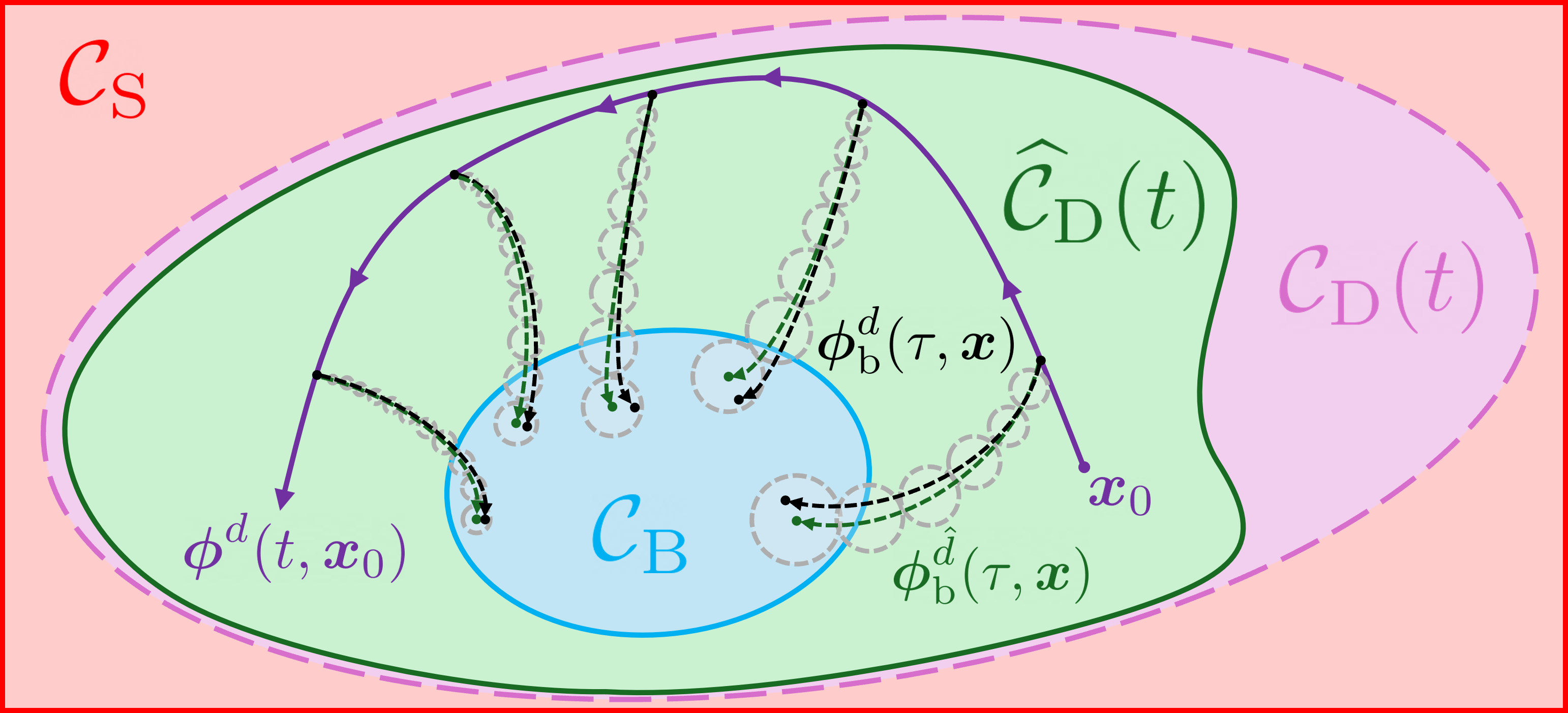
Figure 1: Illustration of the presented robust safety-critical control framework with disturbance observer. The set $\widehat{\mathcal{C}}_{\rm D}(t)$, a known subset of an unknown controlled invariant set $\mathcal{C}_{\rm D}(t)$, is used to guarantee the safety of the disturbed flow $\bm{\phi}^{{d}}(t,\bm{x}_{0})$. A disturbance observer shrinks the uncertainty bounds over time $t$.

Consider a new time-varying set, $\widehat{\mathcal{C}}_{\rm D}(t)$

$$\hskip-7.11317pt\widehat{\mathcal{C}}_{\rm D}(t)\triangleq\left\{\bm{x}\in\mathcal{X}\,\middle|\,\begin{array}[]{c}h(\bm{\phi}^{\hat{d}}_{\rm b}(\tau,\bm{x}))\geq\epsilon_{\tau},\forall\mkern 1.0mu\tau\in[0,T],\\ h_{\rm b}(\bm{\phi}^{\hat{d}}_{\rm b}(T,\bm{x}))\geq\epsilon_{\rm b}\\ \end{array}\right\},$$ (21)

defined by the estimate flow and the tightening terms $\epsilon_{\rm\tau}$ and $\epsilon_{\rm b}$. If these tightening terms are chosen carefully, $\widehat{\mathcal{C}}_{\rm D}(t)$ is a subset of $\mathcal{C}_{\rm D}(t)$, as stated below similar to [17, Lemma 1].

Lemma 3.

Let $\mathcal{L}_{h}$ and $\mathcal{L}_{h_{\rm b}}$ be the Lipschitz constants of $h$ and $h_{\rm b}$, respectively, and let $\delta_{{\rm max}}(\tau,t)$ be a norm bound on the deviation between $\bm{\phi}^{d}_{\rm b}(\tau,\bm{x})$ and $\bm{\phi}^{\hat{d}}_{\rm b}(\tau,\bm{x})$ at backup time $\tau\in[0,T]$ and global time ${t\geq 0}$:

$$\left\|\bm{\phi}^{d}_{\rm b}(\tau,\bm{x})-\bm{\phi}^{\hat{d}}_{\rm b}(\tau,\bm{x})\right\|\leq\delta_{{\rm max}}(\tau,t),$$ (22)

for all $\bm{x}\in\mathcal{C}_{\rm S}$. If $\epsilon_{\tau}\geq\mathcal{L}_{h}\delta_{{\rm max}}(\tau,t)$ and $\epsilon_{\rm b}\geq\mathcal{L}_{h_{\rm b}}\delta_{{\rm max}}(T,t)$ hold for all $\tau\in[0,T]$ and $t\geq 0$, then $\widehat{\mathcal{C}}_{\rm D}(t)\!\subseteq\!\mathcal{C}_{\rm D}(t)$.

Proof.

Consider any state ${\bm{x}\in\widehat{\mathcal{C}}_{\rm D}(t)}$. Membership to $\widehat{\mathcal{C}}_{\rm D}(t)$ implies $h(\bm{\phi}^{\hat{d}}_{\rm b}(\tau,\bm{x}))\geq\epsilon_{\tau}\geq\mathcal{L}_{h}\delta_{{\rm max}}(\tau,t)$. It follows that

$$h(\bm{\phi}^{d}_{\rm b}(\tau,\bm{x})) =h(\bm{\phi}^{\hat{d}}_{\rm b}(\tau,\bm{x}))-\big{(}h(\bm{\phi}^{\hat{d}}_{\rm b}(\tau,\bm{x}))-h(\bm{\phi}^{d}_{\rm b}(\tau,\bm{x}))\big{)}$$

$$\geq\mathcal{L}_{h}\delta_{{\rm max}}(\tau,t)-\big{|}h(\bm{\phi}^{\hat{d}}_{\rm b}(\tau,\bm{x}))-h(\bm{\phi}^{d}_{\rm b}(\tau,\bm{x}))\big{|}.$$

By using the Lipschitz continuity of $h$ and (22), we have

$$|h(\bm{\phi}^{\hat{d}}_{\rm b}(\tau,\bm{x}))-h(\bm{\phi}^{d}_{\rm b}(\tau,\bm{x}))|\leq\mathcal{L}_{h}\delta_{{\rm max}}(\tau,t),$$

meaning that ${h(\bm{\phi}^{d}_{\rm b}(\tau,\bm{x}))\geq 0}$ for any $\bm{x}\in\widehat{\mathcal{C}}_{\rm D}(t)$. Similarly, for any $\bm{x}\in\widehat{\mathcal{C}}_{\rm D}(t)$, the flow with the estimated disturbance satisfies $h_{\rm b}(\bm{\phi}^{\hat{d}}_{\rm b}(T,\bm{x}))\geq\epsilon_{\rm b}\geq\mathcal{L}_{h_{\rm b}}\delta_{{\rm max}}(T,t)$, and

$$|h_{\rm b}(\bm{\phi}^{\hat{d}}_{\rm b}(T,\bm{x}))-h_{\rm b}(\bm{\phi}^{d}_{\rm b}(T,\bm{x}))|\leq\mathcal{L}_{h_{\rm b}}\delta_{{\rm max}}(T,t).$$

This guarantees that ${h_{\rm b}(\bm{\phi}^{d}_{\rm b}(T,\bm{x}))\geq 0}$. Thus, based on (17), ${\bm{x}\in\mathcal{C}_{\rm D}(t)}$ holds for any ${\bm{x}\in\widehat{\mathcal{C}}_{\rm D}(t)}$, so ${\widehat{\mathcal{C}}_{\rm D}(t)\subseteq\mathcal{C}_{\rm D}(t)}$. ∎

Lemma˜3 guides the selection of $\epsilon_{\rm\tau}$ and $\epsilon_{\rm b}$ using a bound $\delta_{\rm max}(\tau,t)$ on the discrepancy between the unknown (disturbed) and estimated flows. To derive such a bound, we first characterize the fidelity of the disturbance estimate.

Lemma 4.

Given a disturbance satisfying ˜1 and a disturbance observer as in (11a), (11b) with error bound $\bar{e}(t)$ as defined in (12), we have

$$\|{\bm{d}(\tau+t)-\hat{\bm{d}}(t)}\|\leq\delta_{v}\tau+\bar{e}(t),$$ (23)

for any global time $t\geq 0$ and backup time $\tau\geq 0$.

Proof.

The triangle inequality implies for any ${t,\tau\geq 0}$ that

$$\|\bm{d}(\tau+t)-\hat{\bm{d}}(t)\| \leq\|\bm{d}(\tau+t)-\bm{d}(t)\|+\|\bm{d}(t)-\hat{\bm{d}}(t)\|,$$

where ${\|\bm{d}(t)-\hat{\bm{d}}(t)\|\leq\bar{e}(t)}$ according to Lemma˜1, and

$$\|\bm{d}(\tau+t)-\bm{d}(t)\|\leq\int_{t}^{\tau+t}\|\dot{\bm{d}}(s)\|\,ds\leq\delta_{v}\tau,$$

because $\|\dot{\bm{d}}(t)\|\leq\delta_{v}$. These inequalities lead to (23). ∎

Now we derive a flow bound as required by Lemma˜3.

Lemma 5.

For systems (13) and (14) let $f_{\rm cl}$ be locally Lipschitz on $\mathcal{X}$ with Lipschitz constant $\mathcal{L}_{\rm cl}$. If ˜1 is satisfied, then (22) holds for all $\tau\in[0,T]$ and $t\geq 0$ with

$$\delta_{\max}(\tau,t)\triangleq\bigg{(}\frac{\delta_{v}}{\mathcal{L}_{\rm cl}^{2}}+\frac{\bar{e}(t)}{\mathcal{L}_{\rm cl}}\bigg{)}\Big{(}{\rm e}^{\mathcal{L}_{\rm cl}\tau}-1\Big{)}-\frac{\delta_{v}}{\mathcal{L}_{\rm cl}}\tau.$$ (24)

Proof.

Introducing ${\Delta\phi(\tau,\bm{x})\triangleq\|\bm{\phi}^{d}_{\rm b}(\tau,\bm{x})-\bm{\phi}^{\hat{d}}_{\rm b}(\tau,\bm{x})\|}$ and expanding the bound between the flows (13) and (14),

$$\Delta\phi(\tau,\bm{x})\leq\!\int^{\tau}_{0}\!\mathcal{L}_{\rm cl}\,\Delta\phi(s,\bm{x})ds+\!\int^{\tau}_{0}\!\big{\|}\bm{d}(s+t)-\hat{\bm{d}}(t)\big{\|}ds.$$

Applying Lemma˜4, we obtain

$$\Delta\phi(\tau,\bm{x})\leq\int^{\tau}_{0}\mathcal{L}_{\rm cl}\,\Delta\phi(s,\bm{x})ds+\frac{\delta_{v}}{2}\tau^{2}+\bar{e}(t)\tau.$$

Using the Gronwall-Bellman Inequality [18, Lemma 2.1],

$$\Delta\phi(\tau,\bm{x})\!\leq\!{\!\int^{\tau}_{0}\!\!\!\Big{(}\frac{\delta_{v}}{2}s^{2}\!+\!\bar{e}(t)s\Big{)}\mathcal{L}_{\rm cl}{\rm e}^{\mathcal{L}_{\rm cl}(\tau-s)}ds\!+\!\frac{\delta_{v}}{2}\tau^{2}\!+\!\bar{e}(t)\tau}.$$

Calculating the integral yields the result. ∎

Remark 1.

While the flow bound $\delta_{\rm max}(\tau,t)$ grows with $\tau$, it shrinks with $t$ if $\bm{\Lambda}$ is chosen such that ${\lambda_{\rm min}>\delta_{v}/\delta_{d}}$, because the estimate of the disturbance improves as $t$ increases (i.e., $\bar{e}(t)$ decreases). The bound in (24) is general, and there may exist tighter problem-specific bounds. For example, the closed-loop backup dynamics can often be made contractive [17] which yields tighter flow bounds [20, Corollary 3.17].

We now state our main result about the set $\widehat{\mathcal{C}}_{\rm D}(t)$, which is comprised only of known terms.

Theorem 2.

Let $\epsilon_{\tau}$ and $\epsilon_{\rm b}$ satisfy ${\epsilon_{\tau}\geq\mathcal{L}_{h}\delta_{{\rm max}}(\tau,t)}$ and ${\epsilon_{\rm b}\geq\mathcal{L}_{h_{\rm b}}\delta_{{\rm max}}(T,t)}$ for all ${\tau\in[0,T]}$ and ${t\geq 0}$, with $\delta_{{\rm max}}(\tau,t)$ defined in (24). For any $\bm{x}\in\widehat{\mathcal{C}}_{\rm D}(t)$, there exists a controller $\bm{u}$ such that ${\bm{\phi}^{d}(\vartheta,\bm{x})\in\mathcal{C}_{\rm D}(t+\vartheta)\subseteq\mathcal{C}_{\rm S},\forall\mkern 1.0mu\vartheta\geq 0}$.

Proof.

By Lemma˜3, ${\bm{x}\in\widehat{\mathcal{C}}_{\rm D}(t)\mkern-6.0mu\implies\bm{x}\in\mathcal{C}_{\rm D}(t)}$, and by Lemma˜2, $\bm{u}_{\rm b}$ ensures ${\bm{\phi}^{d}(\vartheta,\bm{x})\in\mathcal{C}_{\rm D}(t+\vartheta)}$, ${\forall\mkern 2.0mu\vartheta\geq 0}$. ∎

We are now ready to derive control conditions to ensure the robust safety of (10) via the forward invariance of $\widehat{\mathcal{C}}_{\rm D}(t)$ (where ${\widehat{\mathcal{C}}_{\rm D}(t)\subseteq\mathcal{C}_{\rm D}(t)\subseteq\mathcal{C}_{\rm S}}$). From (21), this requires

$$\begin{gathered}\dot{h}(\bm{\phi}^{\hat{d}}_{\rm b}(\tau,\bm{x}),\bm{u})-\frac{\partial\epsilon_{\tau}}{\partial t}\geq-\alpha\big{(}h(\bm{\phi}^{\hat{d}}_{\rm b}(\tau,\bm{x}))-\epsilon_{\tau}\big{)},\\ \dot{h}_{\rm b}(\bm{\phi}^{\hat{d}}_{\rm b}(T,\bm{x}),\bm{u})-\frac{\partial\epsilon_{\rm b}}{\partial t}\geq-\alpha_{\rm b}\big{(}h_{\rm b}(\bm{\phi}^{\hat{d}}_{\rm b}(T,\bm{x}))-\epsilon_{\rm b}\big{)}.\end{gathered}$$

Note that $\epsilon_{\tau}$ and $\epsilon_{\rm b}$ are functions of $t$ and $\tau$. Expanding the total derivatives for system (10) we have for all $\tau\in[0,T]$,

$$\begin{gathered}\hskip-31.2982pt\nabla h(\bm{\phi}^{\hat{d}}_{\rm b}(\tau,\bm{x}))\big{(}\bm{\Phi}(\tau,\bm{x})\dot{\bm{x}}+\bm{\Theta}(\tau,\bm{x}){\dot{{\hat{\bm{d}\mkern 7.0mu}\mkern-7.0mu}{}\mkern 7.0mu}\mkern-7.0mu}{}\mkern 1.0mu\big{)}\geq\\ \hskip 56.9055pt-\alpha\big{(}h(\bm{\phi}^{\hat{d}}_{\rm b}(\tau,\bm{x}))-\epsilon_{\tau}\big{)}+\frac{\partial\epsilon_{\tau}}{\partial t},\\ \hskip-14.22636pt\nabla h_{\rm b}(\bm{\phi}^{\hat{d}}_{\rm b}(T,\bm{x}))\big{(}\bm{\Phi}(T,\bm{x})\dot{\bm{x}}+\bm{\Theta}(T,\bm{x}){\dot{{\hat{\bm{d}\mkern 7.0mu}\mkern-7.0mu}{}\mkern 7.0mu}\mkern-7.0mu}{}\mkern 1.0mu\big{)}\geq\\ \hskip 71.13188pt-\alpha_{\rm b}\big{(}h_{\rm b}(\bm{\phi}^{\hat{d}}_{\rm b}(T,\bm{x}))-\epsilon_{\rm b}\big{)}+\frac{\partial\epsilon_{\rm b}}{\partial t},\end{gathered}$$ (29)

where ${\dot{\bm{x}}=f(\bm{x})+g(\bm{x})\bm{u}+\bm{d}}$. The state-transition matrix, ${\bm{\Phi}(\tau,\bm{x})\triangleq\partial\bm{\phi}^{\hat{d}}_{\rm b}(\tau,\bm{x})/\partial\bm{x}}$, is the solution to

$$\begin{gathered}{\dot{\bm{\Phi}}}(\tau,\bm{x})=F_{\rm cl}(\bm{\phi}^{\hat{d}}_{\rm b}(\tau,\bm{x}))\bm{\Phi}(\tau,\bm{x}),\mkern 9.0mu\bm{\Phi}(0,\bm{x})={\bm{I}},\end{gathered}$$

where ${F_{\rm cl}(\bm{x})}$ is the Jacobian of (14) evaluated at $\bm{\phi}^{\hat{d}}_{\rm b}(\tau,\bm{x})$. Matrix ${\bm{\Theta}(\tau,\bm{x})\triangleq{\partial\bm{\phi}^{\hat{d}}_{\rm b}(\tau,\bm{x})}/{\partial\hat{\bm{d}}}}$, which represents the sensitivity of the flow to the disturbance estimate, is given by

$$\begin{gathered}{\dot{\bm{\Theta}}}(\tau,\bm{x})=F_{\rm cl}(\bm{\phi}^{\hat{d}}_{\rm b}(\tau,\bm{x}))\bm{\Theta}(\tau,\bm{x})+\bm{I},\mkern 9.0mu\bm{\Theta}(0,\bm{x})={\bm{0}}.\end{gathered}$$

Enforcing constraint (29) could ensure the forward invariance of $\widehat{\mathcal{C}}_{\rm D}(t)$ and thereby guarantee safety. However, (29) includes the unknown disturbance $\bm{d}$ in $\dot{\bm{x}}$ and ${\dot{{\hat{\bm{d}\mkern 7.0mu}\mkern-7.0mu}{}\mkern 7.0mu}\mkern-7.0mu}{}$. Thus, we derive sufficient conditions for the satisfaction of (29) with a method inspired by [2]. The following Theorem establishes that controllers satisfying these conditions ensure the robust safety of the system (10) despite the unknown disturbance.

Theorem 3.

Any locally Lipschitz controller $\bm{u}$ satisfying

$$\begin{aligned} \nabla h(\bm{\phi}^{\hat{d}}_{\rm b}(\tau,\bm{x}))\bm{\Phi}(\tau,\bm{x})\big{(}f(\bm{x})+g(\bm{x})\bm{u}+\hat{\bm{d}}\mkern 1.0mu\big{)}\geq\\ -\alpha\big{(}h(\bm{\phi}^{\hat{d}}_{\rm b}(\tau,\bm{x}))-\epsilon_{\tau}\big{)}+\frac{\partial\epsilon_{\tau}}{\partial t}+\rho,\end{aligned}$$ (30a)

$$\begin{aligned} \nabla h_{\rm b}(\bm{\phi}^{\hat{d}}_{\rm b}(T,\bm{x}))\bm{\Phi}(T,\bm{x})\big{(}f(\bm{x})+g(\bm{x})\bm{u}+\hat{\bm{d}}\mkern 1.0mu\big{)}\geq\\ -\alpha_{\rm b}\big{(}h_{\rm b}(\bm{\phi}^{\hat{d}}_{\rm b}(T,\bm{x}))-\epsilon_{\rm b}\big{)}+\frac{\partial\epsilon_{\rm b}}{\partial t}+\rho_{\rm b},\end{aligned}$$ (30b)

for all ${\tau\in[0,T]}$, ${t\geq 0}$, and $\bm{x}\in\mathcal{C}_{\rm S}$, with robustness terms

$$\begin{gathered}\rho\triangleq\bar{e}(t)\left\|\nabla h(\bm{\phi}^{\hat{d}}_{\rm b}(\tau,\bm{x}))\big{(}\bm{\Phi}(\tau,\bm{x})+\bm{\Theta}(\tau,\bm{x})\bm{\Lambda}\big{)}\right\|,\\ \rho_{\rm b}\triangleq\bar{e}(t)\left\|\nabla h_{\rm b}(\bm{\phi}^{\hat{d}}_{\rm b}(T,\bm{x}))\big{(}\bm{\Phi}(T,\bm{x})+\bm{\Theta}(T,\bm{x})\bm{\Lambda}\big{)}\right\|,\end{gathered}$$

renders the set ${\widehat{\mathcal{C}}_{\rm D}(t)\!\subseteq\!\mathcal{C}_{\rm D}(t)\!\subseteq\!\mathcal{C}_{\rm S}}$ forward invariant for (10).

Proof.

Substituting ${\bm{d}=\hat{\bm{d}}+\bm{e}}$ and ${{\dot{{\hat{\bm{d}\mkern 7.0mu}\mkern-7.0mu}{}\mkern 7.0mu}\mkern-7.0mu}{}=\bm{\Lambda}\bm{e}}$ into (29), using the Cauchy-Schwartz inequality and the upper bound ${\|\bm{e}(t)\|\leq\bar{e}(t)}$ from Lemma˜1, it can be shown that the conditions in (30) imply that (29) holds. Applying Theorem˜1 to system (10), the satisfaction of (29) yields the forward invariance of $\widehat{\mathcal{C}}_{\rm D}(t)$. By Lemma˜3, we have ${\widehat{\mathcal{C}}_{\rm D}(t)\subseteq\mathcal{C}_{\rm D}(t)}$. ∎

Theorem˜3 can now be used to develop a novel point-wise optimal safe controller via the proposed Disturbance Observer Backup CBF (DO-bCBF) approach:

$$\bm{u}_{\rm safe}(\bm{x})=\underset{\bm{u}\in\mathcal{U}}{\text{argmin}}\mkern 9.0mu \left\|\bm{u}_{\rm p}-\bm{u}\right\|^{2}\quad$$ (DO-bCBF-QP)

s.t. $$\eqref{eq: mainthmConstraints_cont},\ \eqref{eq: mainthmConstraints_reach},$$

for all ${\tau\in\{0,\Delta,\dots,T\}}$ with discretization step $\Delta$, analogously to the (bCBF-QP). Note that robustness against the discretization of $\tau$ can be achieved based on [16, Thm. 1].

Remark 2.

From Lemma˜2, $\mathcal{C}_{\rm D}(t)$ is controlled invariant, and thus if the (DO-bCBF-QP) becomes infeasible, the robust backup control law $\bm{u}_{\rm b}$ can be used to stay in $\mathcal{C}_{\rm D}(t)$ until the optimization problem becomes feasible again, guaranteeing robust safety since ${\widehat{\mathcal{C}}_{\rm D}(t)\subseteq\mathcal{C}_{\rm D}(t)\subseteq\mathcal{C}_{\rm S}}$ and $\bm{u}_{\rm b}\in\mathcal{U}$. Alternatively, a smooth switching approach could be used as in [21].

IV Numerical Examples

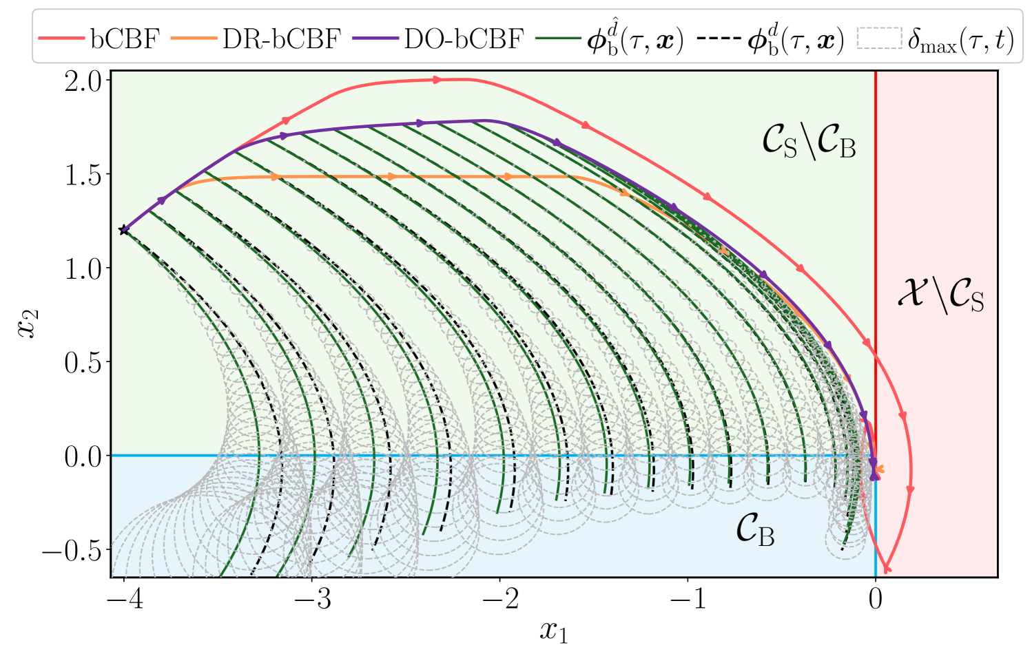
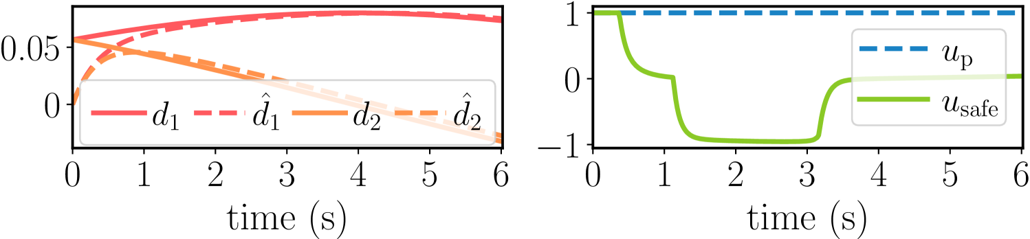
Figure 2: Simulation of the double integrator (31) with ${\omega=0.2}$ using the proposed disturbance observer backup CBF controller (DO-bCBF-QP). The trajectory of the system (purple) indicates safe behavior despite the unknown disturbance (top). The controller uses estimated backup trajectories (green) that approximate the unknown backup flow under the true disturbance (black dashed). The estimation uncertainty decreases over time $t$ thanks to the disturbance observer (see the gray circles centered on the estimated trajectories representing the Gronwall norm balls from Lemma˜5). Indeed, the true disturbance is captured by its estimate (bottom left), while the control input stays bounded (bottom right).

In this section we demonstrate the effectiveness of the proposed approach using two simulation examples.

Example 1.

Consider a double integrator given by

$$\dot{\bm{x}}=\begin{bmatrix}x_{2},u\end{bmatrix}^{T}\mkern-4.0mu+\bm{d}(t),$$ (31)

with position $x_{1}$, velocity $x_{2}$, state ${\bm{x}=[x_{1},x_{2}]^{T}\in\mathbb{R}^{2}}$, and control input ${u\in\mathcal{U}=[-1,1]}$. The safe set is defined as ${\mathcal{C}_{\rm S}\triangleq\{\bm{x}\in\mathbb{R}^{2}:-x_{1}\geq 0\}}$. The unknown disturbance is time-varying, with ${\bm{d}(t)=\delta_{d}\mkern 1.0mu[{\rm sin}{(\mkern-1.0mu\omega t+\frac{\pi}{4})},{\rm cos}{(\mkern-1.0mu\omega t+\frac{\pi}{4})}]^{T}}$, and we use the known bounds ${\left\|\bm{d}\right\|\leq\delta_{d}=0.08}$ and ${\|{\dot{\bm{d}}\|}\leq\delta_{v}=\delta_{d}\omega}$ for control design. The backup control law ${\bm{u}_{\rm b}(\bm{x})=-1}$ brings the system to the backup set ${\mathcal{C}_{\rm B}\triangleq\{\bm{x}\in\mathbb{R}^{2}:-x_{1}\geq 0,-x_{2}\geq 0\}}$. The primary controller, ${\bm{u}_{\rm p}=1}$, drives (31) to the unsafe right half-plane.

We simulate (31) with the proposed (DO-bCBF-QP) controller, and we compare our approach with two baselines: the disturbance-robust backup CBF (DR-bCBF) solution in [17], that is designed for the worst-case disturbance without utilizing a disturbance observer, and the standard (bCBF-QP) reviewed in Section˜II-B, that ignores the disturbance. The results are shown in Fig. 2 for ${\omega=0.2}$ and in Fig. 3 for ${\omega=0}$. Both configurations indicate that the proposed DO-bCBF approach guarantees safety despite the unknown disturbance, and is less conservative (allowing higher velocity $x_{2}$) than the DR-bCBF. In contrast, the bCBF violates safety due to the disturbance. We also depict the disturbed flow $\bm{\phi}^{d}_{\rm b}(\tau,\bm{x})$, the estimated flow $\bm{\phi}^{\hat{d}}_{\rm b}(\tau,\bm{x})$, and its uncertainty bound from Lemma˜5 represented as circles. As time $t$ goes on, the disturbance estimate gets more accurate and the circles shrink. For ${\omega=0}$, the uncertainty vanishes completely, implying that the set $\widehat{\mathcal{C}}_{\rm D}(t)$ approaches $\mathcal{C}_{\rm D}(t)$, since the disturbance is constant and the estimation error converges to zero by Lemma˜1.

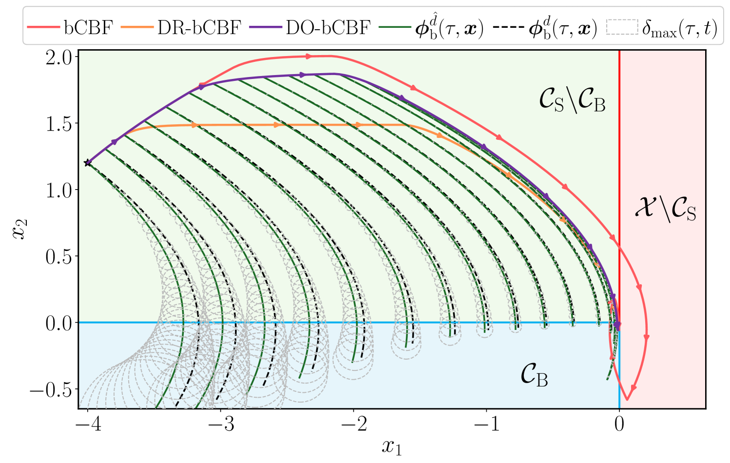
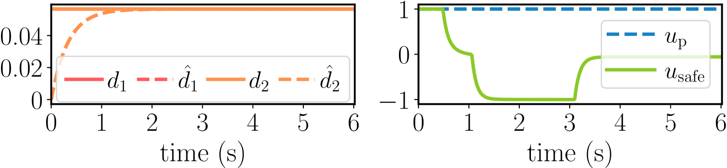
Figure 3: Simulation of the double integrator (31) with ${\omega=0}$ using the disturbance observer backup CBF controller (DO-bCBF-QP).

Example 2.

Consider next a planar quadrotor:

$$\!\underbrace{\begin{bmatrix}\dot{x}\\ \dot{z}\\ \dot{\theta}\\ \ddot{x}\\ \ddot{z}\\ \ddot{\theta}\end{bmatrix}}_{\dot{\bm{x}}}\!=\!\underbrace{\begin{bmatrix}\dot{x}\\ \dot{z}\\ \dot{\theta}\\ 0\\ -g_{\rm D}\\ 0\end{bmatrix}}_{f(\bm{x})}\!+\!\underbrace{\begin{bmatrix}0&0\\ 0&0\\ 0&0\\ {\rm sin}(\theta)/m&0\\ {\rm cos}(\theta)/m&0\\ 0&-1/J\\ \end{bmatrix}}_{g(\bm{x})}\!\!\underbrace{\begin{bmatrix}F\\ M\end{bmatrix}}_{\bm{u}}\!+\!\underbrace{\begin{bmatrix}0\\ 0\\ 0\\ d_{4}(t)\\ d_{5}(t)\\ 0\end{bmatrix}}_{\bm{d}(t)}\!,$$ (32)

where $x$ and $z$ denote horizontal position and altitude in an inertial reference frame, respectively, and $\theta$ is the pitch angle. The state is ${\bm{x}\in\mathcal{X}\triangleq\mathbb{R}^{2}\times\mathbb{S}^{1}\times\mathbb{R}^{3}}$ and the inputs are the thrust ${F\in[0,F_{\rm max}]}$ and moment ${M\in[-M_{\rm max},M_{\rm max}]}$ applied by the propellers. Here, ${g_{\rm D}=9.81\mkern 2.0mu{\rm m/s^{2}}}$ is the acceleration due to gravity, ${m={\rm 1\mkern 2.0mukg}}$ is the mass of the quadrotor, and ${J={\rm 0.25\mkern 2.0mukg\mkern 1.0mum^{2}}}$ is the principal moment of inertia about the $y$-axis. The components of the disturbance are given by ${d_{4}(t)=1\mkern 2.0mu{\rm m/s^{2}}}$ and ${d_{5}(t)=\frac{1}{2}{\rm sin}(0.3t-\frac{\pi}{3})\mkern 2.0mu{\rm m/s^{2}}}$.

We consider the motivating case where a human operator loses connection with the quadrotor [21], such that ${\bm{u}_{\rm p}=\bm{0}}$, and the controller must prevent crashing into the ground. The safe set ${\mathcal{C}_{\rm S}\triangleq\{\bm{x}\in\mathcal{X}:h(\bm{x})=z-z_{\rm min}\geq 0\}}$ is thus defined by a minimum altitude ${z_{\rm min}>0}$. The backup control law ${\bm{u}_{\rm b}(\bm{x})=[F_{\rm max},K_{\rm p}\theta+K_{\rm d}\dot{\theta}]^{T}}$, with gains ${K_{\rm p},K_{\rm d}>0}$, aims to bring the quadrotor to horizontal and apply maximum thrust to prevent a crash. The backup set is defined by ${\mathcal{C}_{\rm B}\triangleq\{\bm{x}\in\mathcal{X}:h_{\rm b}(\bm{x}),h(\bm{x})\geq 0\}}$. The function ${h_{\rm b}(\bm{x})=-\frac{1}{\kappa}\ln\big{(}{\rm e}^{-\kappa h_{1}(\bm{x})}+{\rm e}^{-\kappa h_{2}(\bm{x})}+{\rm e}^{-\kappa h_{3}(\bm{x})}\big{)}}$ with ${\kappa>0}$ under-approximates ${\min\{h_{1}(\bm{x}),h_{2}(\bm{x}),h_{3}(\bm{x})\}}$, as in [22, 23], with ${h_{1}(\bm{x})=\dot{z}}$, ${h_{2}(\bm{x})=\theta^{2}_{\rm max}-\theta^{2}}$, and ${h_{3}(\bm{x})=\dot{\theta}^{2}_{\rm max}-\dot{\theta}^{2}}$, where ${{\theta}_{\rm max},\dot{\theta}_{\rm max}>0}$. It can be shown that $\bm{u}_{\rm b}(\bm{x})$ renders $\mathcal{C}_{\rm B}$ robustly forward invariant and satisfies input constraints if ${F_{\rm max}\geq\frac{m(g_{\rm D}+\delta_{d})}{{\rm cos}(\theta_{\rm max})}}$, ${K_{\rm d}^{2}>4JK_{\rm p}}$, and ${M_{\rm max}\geq K_{\rm p}\theta_{\rm max}+K_{\rm d}\dot{\theta}_{\rm max}}$. We omit the proof for brevity. We use a problem-specific flow bound, where in (24), $\mathcal{L}_{\rm cl}$ is replaced with an upper bound of the log norm of $F_{\rm cl}$.

Figure˜4 shows the simulation results for system (32) with the proposed (DO-bCBF-QP) controller. In the simulation, similar behavior is observed for the nonlinear and higher-dimensional quadrotor dynamics as for the double integrator. The proposed controller ensures robust safety, i.e., prevents the quadrotor from crashing, even in the presence of disturbances while satisfying input constraints. This behavior is achieved using an estimate of the disturbance which is improved over time via the disturbance observer (11a)-(11b).

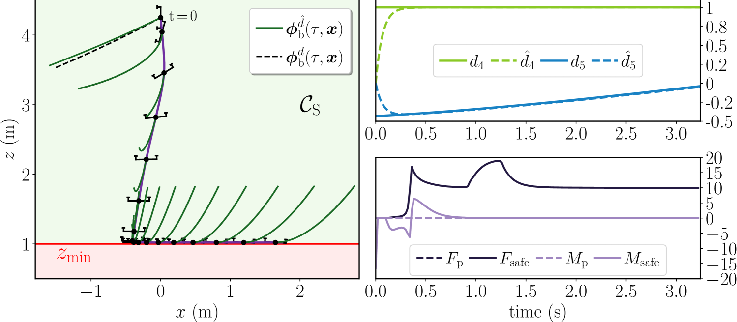
Figure 4: Simulation of the quadrotor (32) using the proposed disturbance observer backup CBF controller (DO-bCBF-QP). The trajectory of the system (purple) indicates safe behavior despite the unknown disturbance (left). The controller uses the estimated backup trajectories (green) that approach the unknown backup trajectories under the true disturbance (black dashed). The disturbance estimate converges to the true value (top right), while the control inputs stay within the prescribed bounds (bottom right).

V Conclusion

We presented a novel framework to guarantee online controlled invariance in the presence of unknown bounded disturbances for input constrained systems. We used a disturbance observer to reduce conservatism and provided forward invariance conditions for a subset of a controlled invariant set considering the disturbed system. We proved that enforcing these conditions guarantees safety for the disturbed system.

References

- [1] A. D. Ames, X. Xu, J. W. Grizzle, and P. Tabuada, “Control barrier function based quadratic programs for safety critical systems,” IEEE Trans. Autom. Control, vol. 62, no. 8, pp. 3861–3876, 2017.
- [2] M. Jankovic, “Robust control barrier functions for constrained stabilization of nonlinear systems,” Automatica, vol. 96, pp. 359–367, 2018.
- [3] K. Garg and D. Panagou, “Robust Control Barrier and Control Lyapunov Functions with Fixed-Time Convergence Guarantees,” in Proc. Amer. Control Conf., pp. 2292–2297, 2021.
- [4] W. Shaw Cortez, D. Oetomo, C. Manzie, and P. Choong, “Control Barrier Functions for Mechanical Systems: Theory and Application to Robotic Grasping,” IEEE Trans. Control Syst. Technol., vol. 29, no. 2, pp. 530–545, 2021.
- [5] E. Daş and R. M. Murray, “Robust safe control synthesis with disturbance observer-based control barrier functions,” in Proc. 61st IEEE Conf. Decision and Control, pp. 5566–5573, 2022.
- [6] E. Daş and J. W. Burdick, “Robust control barrier functions using uncertainty estimation with application to mobile robots,” IEEE Trans. Autom. Control, pp. 1–8, 2025.
- [7] Y. Wang and X. Xu, “Disturbance observer-based robust control barrier functions,” in Proc. Amer. Control Conf., pp. 3681–3687, 2023.
- [8] A. Isaly, O. S. Patil, H. M. Sweatland, R. G. Sanfelice, and W. E. Dixon, “Adaptive safety with a rise-based disturbance observer,” IEEE Trans. Autom. Control, vol. 69, no. 7, pp. 4883–4890, 2024.
- [9] B. T. Lopez, J.-J. E. Slotine, and J. P. How, “Robust adaptive control barrier functions: An adaptive and data-driven approach to safety,” IEEE Control Syst. Lett., vol. 5, no. 3, pp. 1031–1036, 2021.
- [10] Y. Emam, P. Glotfelter, S. Wilson, G. Notomista, and M. Egerstedt, “Data-driven robust barrier functions for safe, long-term operation,” IEEE Trans. on Robotics, vol. 38, no. 3, pp. 1671–1685, 2022.
- [11] L. Lindemann, A. Robey, L. Jiang, S. Das, S. Tu, and N. Matni, “Learning robust output control barrier functions from safe expert demonstrations,” IEEE Open J. Control Syst., vol. 3, pp. 158–172, 2024.
- [12] M. Z. Romdlony and B. Jayawardhana, “On the new notion of input-to-state safety,” in 55th IEEE Conf. Decision and Control, pp. 6403–6409, 2016.
- [13] S. Kolathaya and A. D. Ames, “Input-to-state safety with control barrier functions,” IEEE Control Syst. Lett., vol. 3, no. 1, pp. 108–113, 2019.
- [14] A. Alan, A. J. Taylor, C. R. He, G. Orosz, and A. D. Ames, “Safe controller synthesis with tunable input-to-state safe control barrier functions,” IEEE Control Syst. Lett., vol. 6, pp. 908–913, 2022.
- [15] T. Gurriet, M. Mote, A. D. Ames, and E. Feron, “An Online Approach to Active Set Invariance,” in Proc. 57th IEEE Conf. Decision and Control, pp. 3592–3599, 2018.
- [16] T. Gurriet, M. Mote, A. Singletary, P. Nilsson, E. Feron, and A. D. Ames, “A scalable safety critical control framework for nonlinear systems,” IEEE Access, vol. 8, pp. 187249–187275, 2020.
- [17] D. E. J. van Wijk, S. Coogan, T. G. Molnar, M. Majji, and K. L. Hobbs, “Disturbance-robust backup control barrier functions: Safety under uncertain dynamics,” IEEE Control Syst. Lett., vol. 8, pp. 2817–2822, 2024.
- [18] H. Khalil, Nonlinear Systems. Pearson Education, Prentice Hall, 2 ed., 2002.
- [19] F. Blanchini and S. Miani, Set-Theoretic Methods in Control. Systems & Control: Foundations & Applications, Cham: Springer International Publishing, second ed., 2015.
- [20] F. Bullo, Contraction Theory for Dynamical Systems. Kindle Direct Publishing, 1.1 ed., 2023.
- [21] A. Singletary, A. Swann, Y. Chen, and A. D. Ames, “Onboard safety guarantees for racing drones: High-speed geofencing with control barrier functions,” IEEE Robot. Autom. Lett., vol. 7, no. 2, pp. 2897–2904, 2022.
- [22] L. Lindemann and D. V. Dimarogonas, “Control barrier functions for signal temporal logic tasks,” IEEE Control Syst. Lett., vol. 3, no. 1, pp. 96–101, 2019.
- [23] T. G. Molnar and A. D. Ames, “Composing control barrier functions for complex safety specifications,” IEEE Control Syst. Lett., vol. 7, pp. 3615–3620, 2023.