Convergence Rate Analysis of the Join-the-Shortest-Queue System

Yuanzhe Ma Department of Industrial Engineering and Operations Research, Columbia University, ym2865@columbia.edu Siva Theja Maguluri Department of Industrial and Systems Engineering, Georgia Institute of Technology, siva.theja@gatech.edu

The Join-the-Shortest-Queue (JSQ) policy is among the most widely used routing algorithms for load balancing systems and has been extensively studied. Despite its simplicity and optimality, exact characterization of the system remains challenging. Most prior research has focused on analyzing its performance in steady-state in certain asymptotic regimes such as the heavy-traffic regime. However, the convergence rate to the steady-state in these regimes is often slow, calling into question the reliability of analyses based solely on the steady-state and heavy-traffic approximations. To address this limitation, we provide a finite-time convergence rate analysis of a JSQ system with two symmetric servers. In sharp contrast to the existing literature, we directly study the original system as opposed to an approximate limiting system such as a diffusion approximation. Our results demonstrate that for such a system, the convergence rate to its steady-state, measured in the total variation distance, is $O\left(\frac{1}{(1-\rho)^{3}}\frac{1}{t}\right)$, where $\rho\in(0,1)$ is the traffic intensity.

Join-the-shortest-queue; Load Balancing System; Transient Analysis; Coupling

1 Introduction

Efficient load balancing is central for optimizing resource allocation and minimizing job delays in modern service systems and data centers. The Join–the-Shortest-Queue (JSQ) policy is a popular routing algorithm used in load balancing systems due to its simplicity and optimality under various criteria. Starting from its introduction by Winston [38], it received significant attention over the decades. However, the analysis of the JSQ system is quite nontrivial. Even for simple models involving only two queues, there is extensive literature that analyzes their exact performance [20, 24, 7, 14, 2]. For systems with more than two queues, there are only some approximation results.

Due to the complexity of problem, most prior works consider a JSQ system only under its steady state. Further, analysis is typically conducted in some asymptotic regimes, such as the heavy-traffic regime. For example, there are various bounds for the queue length of a JSQ system under its steady state, such as [32, Theorem 10.2.3]. However, modern data centers often appear to be time-variant [4]. This necessitates a careful and precise analysis of the performance of the JSQ system under a finite time $t$ instead of simply analyzing it through its steady state. Motivated by this, we focus on analyzing the transient behavior of a JSQ system. As a starting point, we consider a system consisting of two servers with both arrival and service time following exponential distributions. We analyze its non-asymptotic convergence rate toward its steady state.

As discussed, prior works focus on analyzing the JSQ policy under heavy-traffic regimes and in steady state. However, unsurprisingly, simulation results in Figure 1 reveal that the convergence rate of a JSQ system can be quite slow when the traffic intensity $\rho$ approaches 1. Thus, to conduct a reliable analysis of the JSQ systems, we need to understand their transient behaviors. In addition, prior results also are not applicable to light-traffic settings since State Space Collapse (SSC) is only associated with heavy-traffic regimes. In this paper, we close this gap and obtain an explicit upper bound on the difference between the transient distribution of a JSQ system and its steady state for any $\rho\in(0,1)$.

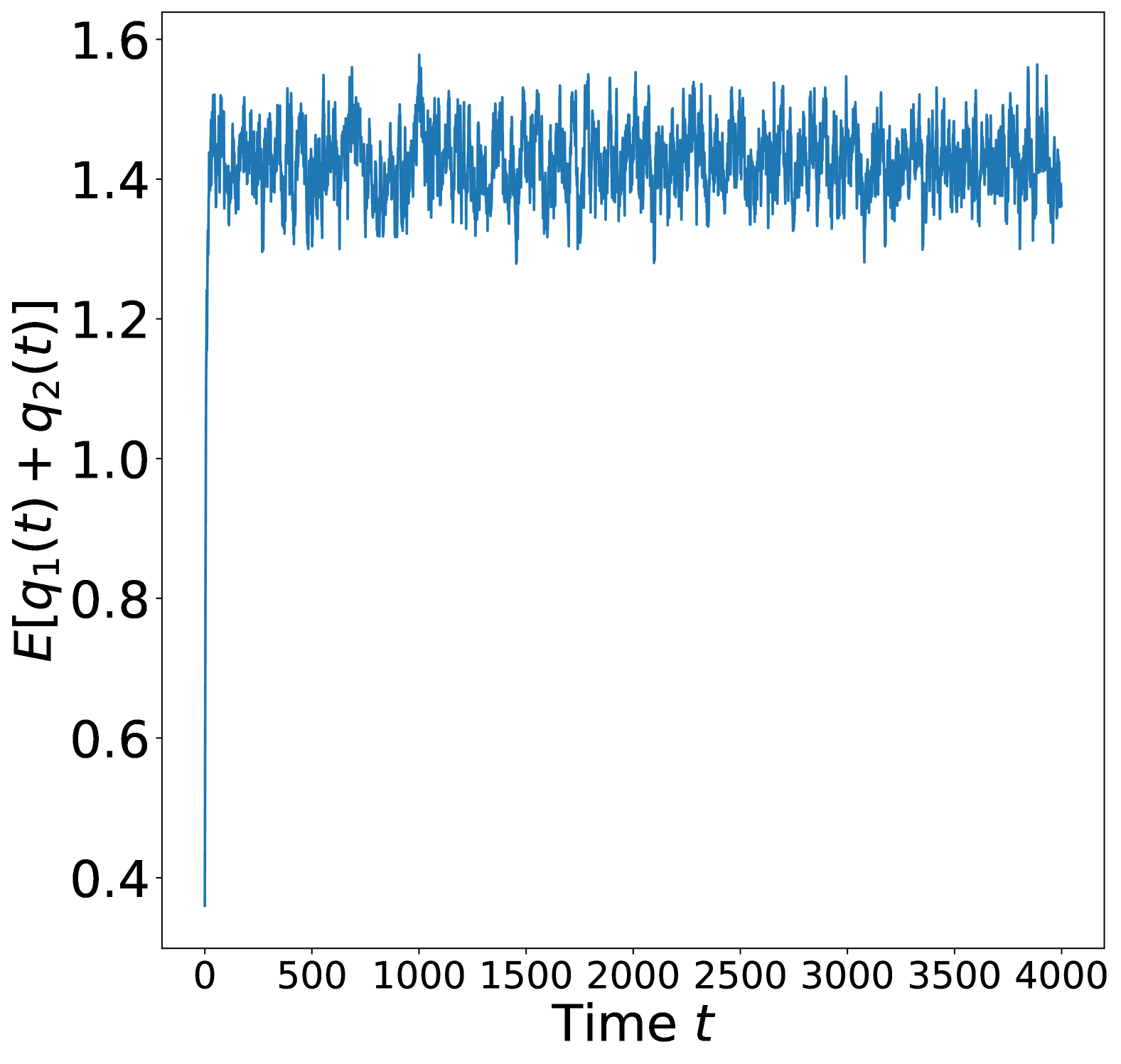
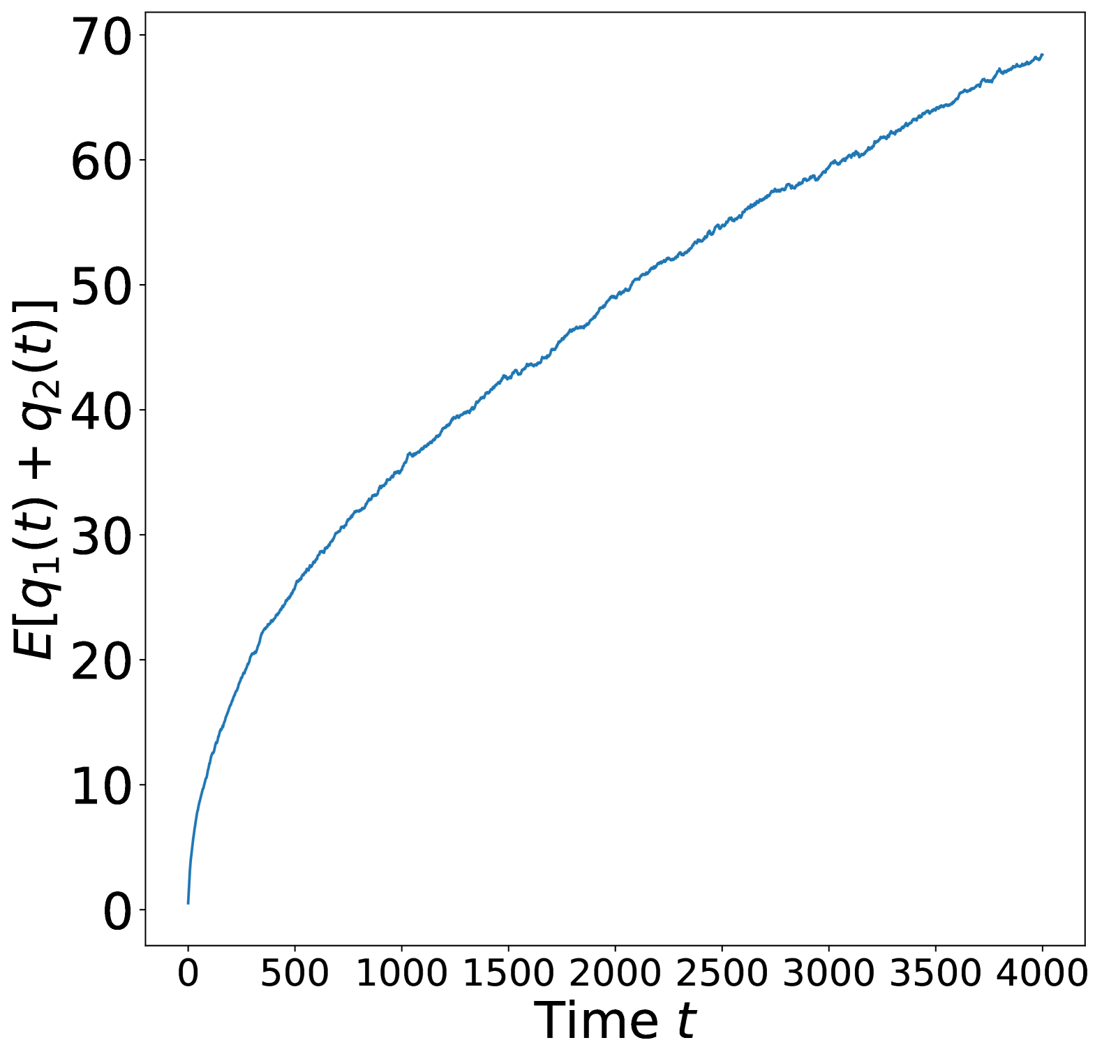
Figure 1: Finite-time performance of a JSQ system at different values of $\rho$, where $q_{i}(t)$ denotes the queue length at time $t$ for server $i$. The results are based on 1000 simulations of trajectories to estimate the sum of the expected queue length vectors. Here we consider a JSQ system with Poisson arrival process with rate $\rho$ and two homogeneous servers following $\mathsf{Exp}\left(1\right)$ with traffic intensity $\rho=0.5$ (the left figure) and $\rho=0.999$ (the right figure), respectively. The pair of plots clearly show that the convergence rates of JSQ systems heavily depend on $\rho$.

In this paper, we focus on analyzing the distribution of the queue length vector, $\mathbb{P}^{t}_{\bm{x}}$, at time $t$, for a JSQ system with initial queue length $\bm{x}$. In particular, we consider its total variation distance to the steady state $\pi$ at every time $t\geq 0$. The total variation (TV) distance is a common metric quantifying the convergence rate of a stochastic system and is known to be closely connected to many other metrics. For example, bounds on TV distances imply bounds on Hellinger metrics. In addition to the TV distance, we also develop the convergence rate of the mean queue length. Using coupling, the key challenge in our method is to obtain an upper bound of the expected hitting times or first passage times of the JSQ system. For general continuous-time Markov chains (CTMC), analyzing the hitting time usually requires extensive exploitation of the structure of the CTMC [11]. In this work, we use several structures of the JSQ system, and show that the problem can be reduced to providing an upper bound on $\mathbb{E}[T_{0}]$, where $T_{0}$ defined in (3.1) is the time it takes for a JSQ system’s queue length vector to hit the origin starting from state $(1,0)$. Through upper bounding $\mathbb{E}[T_{0}]$, we then use the Markov’s inequality to arrive at a bound on $d_{\mathrm{TV}}\left(\mathbb{P}^{t}_{\bm{x}},\pi\right)$.

1.1 Main contribution

Our main result is for a continuous-time JSQ system with two symmetric queues with service time and arrival time both following exponential distributions. We derive an upper bound on $d_{\mathrm{TV}}\left(\mathbb{P}^{t}_{\bm{x}},\pi\right)$ and, as a corollary, an upper bound on the difference between the mean queue length at time $t$ and its steady-state value. These two distances converge to 0 as $t\to\infty$ for any $\rho=\frac{\lambda}{2\mu}\in(0,1)$. In particular, for the TV distance, our convergence rate is

$$O\left(\frac{1}{(1-\rho)^{3}}\frac{1}{t}\right).$$

In contrast to prior work built on diffusion limits, we derive transient bounds by directly studying the original JSQ system, thus avoiding approximation errors. We adopt the coupling method that is commonly used to study Markov chain mixing, which is based on hitting times analysis. We are the first to provide an analysis of transient behavior for a JSQ system for any $\rho\in(0,1)$.

The rest of the paper is organized as follows. We first discuss related work in Section 1.2 as well as notations in Section 1.3. We present the model and our main result in Section 2.1. Our main result consists of the convergence rate in total variation distance, as stated in Theorem 1, and the convergence rate of the mean queue length, as given in Corollary 1. Then we discuss the proof outline in Section 3 while leaving some technical details to the appendix. Finally, we provide concluding remarks and fruitful future directions in Section 4.

1.2 Related work

Since the pioneering work of Winston [38], the JSQ policy has been extensively studied in the literature [8]. In particular, many studies have examined the optimality of the JSQ policy. In [38], it is shown that the JSQ policy is optimal if the service time is identically distributed as exponential random variables and arrival process is a Poisson process. Here, optimality means that the JSQ policy maximizes, with respect to the usual stochastic order, the discounted number of customers with service completed in every fixed time interval. Another result similar to [38] is extended in [37], which explores whether the JSQ policy remains optimal under the same sense, allowing for general arrival distributions and service distributions with non-decreasing hazard rate functions. In [29], it is shown that the JSQ policy minimizes the waiting time of the first $k$ customers for any $k$, under the assumption of having a finite state. Optimality and robustness of the JSQ policy under other criteria are discussed in [6, 28].

As mentioned before, steady-state behaviors of JSQ systems are studied under certain regimes. One popular regime is the heavy-traffic regime, where the arrival rate increases to the maximum capacity with a fixed number of servers. The JSQ policy is known to minimize the average delay in heavy-traffic in [15]. In particular, when there are $K$ queues, in heavy-traffic, and when $t\to\infty$, the performance of the JSQ policy is very close to an $M/M/K$ system with a central queue. To analyze the queue length under the steady state, one can use the techniques based on drift functions [13]. Moment generating function (MGF) methods are known to be quite effective to analyze system in heavy-traffic in steady state. For instance, there are results for discrete-time heavy-traffic JSQ systems based on MGF methods [22].

Other interesting regimes are typically characterized by a parameter $\alpha>0$, which indicates that the scaling of the total service rate minus the total arrival rate is given by $N^{1-\alpha}$, where $N$ is the number of servers. The Sub-Halfin-Whitt regime corresponds to $\alpha\in(0,\frac{1}{2})$, while the Halfin-Whitt regime occurs at $\alpha=\frac{1}{2}$. For a comprehensive survey of recent advances in JSQ systems and detailed analyses of steady states of these regimes, readers may refer to [9, 23].

Transient analyses are generally more complicated than steady-state analyses, even for simple systems such as $M/M/1$ queues [33, 1]. There are known numerical results for transient analysis of JSQ systems [19], but few theoretical results are known regarding their convergence rates. In this work, we analyze the transient behavior through a hitting time analysis (see, e.g., [25]). Though there are some known results related to hitting times or first passage times for a JSQ system [39, 34], they cannot directly be used for our problem. For a simple system such as an $M/M/1$ system, moment generating function (MGF) of the hitting time for the queue length to hit state $0$ is obtained using a construction of an exponential martingale and the optional stopping theorem [31, Proposition 5.4]. One of the key reasons this works is the special property of an $M/M/1$ queue: starting from state $x\geq 1$, the queue length must first hit states $x-1,x-2,\cdots,1$ before hitting state 0. However, this property is not true for a JSQ system. For example, consider a JSQ system with initial queue length $(5,4)$, then it is possible that the queue length vector never hits state $(4,3)$ before hitting $(0,0)$. This is one of the technical barriers to analyze a JSQ system. One may attempt to use the exponential martingale constructed in [34], which also seems challenging. In [34], the objective is to study the hitting time of $(K,K),K\geq 1$ for a JSQ system. One fact exploited in that paper is that a continuous-time JSQ system cannot hit any state $(x_{1},x_{2})$ with $\max\left\{x_{1},x_{2}\right\}>K$ before hitting state $(K,K)$. However, we are mainly interested in the hitting time of $(0,0)$ to obtain the convergence rate of a JSQ system, which is a very different problem, and thus the results in [34] are not applicable.

The convergence rate of a stochastic system and hitting time analysis based on Foster-Lyapunov drift functions has been extensively discussed in the literature, see e.g., [21, 12, 27]. For example, one may use Theorem 2 of [27], which provides a general framework for obtaining exponential convergence rates of general stochastic systems. However, such approach requires constructing a drift function, and it is unclear how to construct such a drift function for a JSQ system. Relatedly, transient analysis for queues has been discussed under various limiting regimes or considering simpler systems [36, 17, 16]. In addition, arising as diffusion limits, explicit convergence rates of reflected Brownian motions have also been analyzed [18, 3, 5]. Compared to these works, we analyze the JSQ system in a fixed system setting.

1.3 Notations

In this section, we introduce the notations that will be used for this paper. We use $\mathbb{P}\left(A\right)$ to denote the probability that event $A$ occurs, and use $\mathbb{E}[X]$ to denote the expected value of the random variable $X$. For a vector $\bm{x}$, we use $x_{i}$ to indicate its $i$-th element. Given two vectors $\bm{x}$ and $\bm{y}$ in $\mathbb{R}^{n}$, we say $\bm{x}\geq\bm{y}$ if $x_{i}\geq y_{i}$ for every $i\in\{1,\ldots,n\}$. For a stochastic process $(X_{t})_{t\geq 0}$ with steady state $\pi$, we use $\mathbb{E}_{\pi}[X]$ and $\mathbb{P}_{\pi}(\cdot)$ to denote the expectation and distribution of $X_{t}$ with respect to the steady state. For two random variables $A$ and $B$, we write $A$ and $B$ equals in distribution, or $A{\buildrel d\over{=}}B$, if $\mathbb{P}\left(A\leq x\right)=\mathbb{P}\left(B\leq x\right)$ for all $x\in\mathbb{R}$. We define $A$ to be stochastically dominated by $B$, or $A\preceq B$, if and only if $\mathbb{P}\left(A>x\right)\leq\mathbb{P}\left(B>x\right)$ for all $x\in\mathbb{R}$. Equivalently, $\mathbb{E}[u(A)]\leq\mathbb{E}[u(B)]$ for all non-decreasing functions $u$. For two probability distributions $\mathbb{P}$ and $\mathbb{Q}$ defined on the sigma-algebra $\mathcal{F}$, we denote the total variation distance between $\mathbb{P}$ and $\mathbb{Q}$ as $d_{\mathrm{TV}}\left(\mathbb{P},\mathbb{Q}\right)=\sup_{A\in\mathcal{F}}|\mathbb{P}(A)-\mathbb{Q}(A)|.$

2 Model and results

2.1 Model

Throughout the paper, we consider a continuous-time load balancing system operating under the JSQ policy. It consists of two single-server queues, and each has infinite capacity. Jobs arrive according to a Poisson process with rate $\lambda$ and service times for each queue are independent exponential random variables with mean $\frac{1}{\mu}$. In addition, arriving jobs will stay in line in case the server is busy. We use $q_{i}(t),i\in\{1,2\}$ to denote the number of jobs in the $i^{\mathrm{th}}$ queue at the beginning of time $t$. Let $\bm{q}(t)\in\mathbb{Z}_{+}^{2}=\left\{0,1,2,3\cdots\right\}^{2}$ be the queue length process with elements $(q_{1}(t),q_{2}(t))$. The JSQ policy sends each arrival to the queue with the least number of jobs, and picks the one with the smaller index when there is a tie. We define $i^{\star}(t)$ as $i^{\star}(t)\in\min\left\{\underset{i\in\{1,2\}}{\argmin}\left\{q_{i}(t)\right\}\right\}.$

The queue length process $\{\bm{q}(t):t\geq 0\}$ is a CTMC with generator matrix $G$ defined as

$$G_{\bm{q},\bm{q}^{\prime}}=\begin{cases}\mu&\mathrm{if\leavevmode\nobreak\ }q_{i}>0\mathrm{\leavevmode\nobreak\ and\leavevmode\nobreak\ }\bm{q}^{\prime}=\bm{q}-\bm{e}^{(i)}\mathrm{\leavevmode\nobreak\ for\leavevmode\nobreak\ }i\in\{1,2\},\\ \lambda&\mathrm{if\leavevmode\nobreak\ }\bm{q}^{\prime}=\bm{q}+\bm{e}^{(i^{\star}(t))},\\ -(\lambda+\mu\sum_{i=1}^{2}\mathbb{I}_{\left\{q_{i}>0\right\}})&\mathrm{if\leavevmode\nobreak\ }\bm{q}=\bm{q}^{\prime},\\ 0&\mathrm{otherwise,}\\ \end{cases},$$

where $\bm{e}^{(i)}$ is the $i$-th unit vector.

2.2 Main result

We now present the main result of this paper: the convergence rate for the queueing system with two queues under the JSQ policy. Our method is based on hitting time analysis and is inspired by the proof of Proposition 5.4 of [31].

As discussed, we use the total variation distance to quantify the convergence rate, as it is the one of the most common metrics. Furthermore, standard results, e.g., Proposition 4.2 of [25], show that $d_{\mathrm{TV}}\left(\mathbb{P},\mathbb{Q}\right)=\frac{1}{2}\sum_{x\in\mathcal{X}}|\mathbb{P}(x)-\mathbb{Q}(x)|$ for any discrete distributions $\mathbb{P},\mathbb{Q}$.

Theorem 1

Consider a JSQ system as described in Section 2.1 with $\rho=\frac{\lambda}{2\mu}<1$. Let the initial state of the queue length be $\bm{x}$ and $\mathbb{P}_{\bm{x}}^{t}$ be the distribution of its queue length vector $\bm{q}(t)$ at time $t$, and let $\pi$ be its steady state, then for all $t>0$,

$$d_{\mathrm{TV}}\left(\mathbb{P}_{\bm{x}}^{t},\pi\right)\leq\frac{1}{t}C_{1}(\lambda,\mu,\bm{x}),$$ (2.1)

where

$$C_{1}(\lambda,\mu,\bm{x})=\frac{2}{\lambda(1-\rho)^{3}}\Big{(}(x_{1}+x_{2})(1-\rho)+\rho(2-\rho)\Big{)}\cdot K(\rho),$$ (2.2)

and $K(\rho)$ is a constant defined as

$$K(\rho)=\begin{cases}\min\left\{1,\frac{(2\rho^{2}+2\rho)(1-\rho^{2})}{(1-2\rho^{2})}\right\},\mathrm{\leavevmode\nobreak\ if\leavevmode\nobreak\ }\rho\in[0,\frac{1}{\sqrt{2}}),\\ 1,\mathrm{\leavevmode\nobreak\ if\leavevmode\nobreak\ }\rho\in[\frac{1}{\sqrt{2}},1)\end{cases}.$$ (2.3)

Note that $K(\rho)\leq 1$ and $K(\rho)=1$ for $\rho\geq 0.33$.

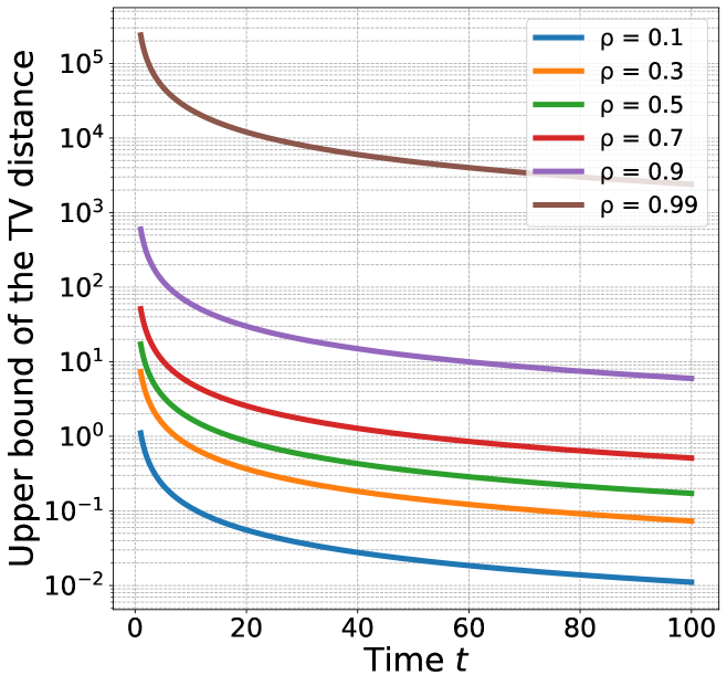
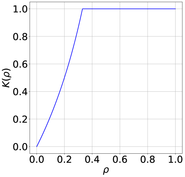
Figure 2: Left: plot of the bound (2.1) as a function of $t$ for different values of $\rho$ and $x_{1}=x_{2}=10,\lambda=10$. Right: plot of $K(\rho)$ (2.3) as a function of $\rho$.

We now visualize the upper bound (2.1) and $K(\rho)$ (2.3) in Figure 2. As we observe, the right-hand-side of (2.1) varies significantly across $\rho$, though its dependence on $t$ is the same for all $\rho$. Our main result, Theorem 1, states that the convergence rate of the JSQ system is at least $\frac{1}{t}$ and there is a constant that is of order $O\left(\frac{1}{(1-\rho)^{3}}\right)$. Our result clearly shows that the finite-time convergence rate depends crucially on the traffic intensity $\rho$ and the arrival rate $\lambda$.

Next, using the below corollary with existing known upper bounds of the JSQ system, e.g., Proposition 4 of [10], we obtain a transient upper bound on the mean queue length. The below bound states that the mean queue length converges at the rate of $O\left(\frac{1}{(1-\sqrt{\rho})^{5}}\frac{1}{\sqrt{t}}\right)$ with proof outline given in Section 3.4.

Corollary 1

Consider a load balancing system under the JSQ policy as described in Section 1 with $\rho=\frac{\lambda}{2\mu}<1$. Let the initial state of the queue length be $\bm{x}$ and let $\pi$ be its steady state, then

$$\mathbb{E}[q_{1}(t)+q_{2}(t)]\leq\frac{\rho(2-\rho)}{1-\rho}+\frac{1}{\sqrt{t}}\Big{(}2C_{1}(\lambda,\mu,\bm{x})+C_{2}(\lambda,\mu,\bm{x})+\frac{2\rho(1+\rho)}{(1-\rho)^{2}}\Big{)}+\frac{2}{t}C_{1}(\lambda,\mu,\bm{x}),$$ (2.4)

where $C_{1}(\lambda,\mu,\bm{x})$ is defined in (2.2) and

$$C_{2}(\lambda,\mu,\bm{x})=(x_{1}^{2}+x_{2}^{2})+2(x_{1}+x_{2})\left[\frac{\sqrt{\rho}(1+\sqrt{\rho})^{2}}{(1-\sqrt{\rho})^{4}}+\frac{\rho}{1-\rho}\right]+2\left[2\frac{\sqrt{\rho}(1+\sqrt{\rho})^{3}}{(1-\sqrt{\rho})^{5}}+\frac{\rho(1+\rho)}{(1-\rho)^{2}}\right].$$ (2.5)

3 Proof of Theorem 1

In the proof, we heavily use the following hitting time denoted by $T_{0}$. Consider a JSQ system with queue length process $\bm{q}(t)$. We define

$$T_{0} =\inf\left\{t>0:\bm{q}(t)=(0,0)\mid\bm{q}(0)=(1,0)\right\}$$ (3.1)

as the time for the queue length process to hit state $(0,0)$ starting from $(1,0)$. In the proof, we also extensively use two coupled processes defined below.

3.1 Coupling with arrival and service

Consider two load balancing systems under the JSQ policy with queue length vectors $\bm{p}(t)$ and $\bm{q}(t)$ as described in Section 1. We say them to be coupled with arrival and service if they can be constructed using $\mathcal{N}_{a}$ and $\mathcal{N}_{d}^{i}$, $i=1,2$, where $\mathcal{N}_{a}$ is a Poisson process with rate $\lambda$ and $\mathcal{N}_{d}^{1},\mathcal{N}_{d}^{2}$ are two Poisson processes with rate $\mu$. We also assume $\mathcal{N}_{a}$, $\mathcal{N}_{d}^{1}$, and $\mathcal{N}_{d}^{2}$ are independent of each other. We interpret $\mathcal{N}_{a}$ as the arrival process and $\mathcal{N}_{d}^{1},\mathcal{N}_{d}^{2}$ as the service process. Therefore, we can write the expressions of increments of the two load balancing systems as

$$\begin{split}dp_{1}(t)=\mathbb{I}_{\left\{p_{1}(t-)\leq p_{2}(t-)\right\}}\mathcal{N}_{a}(dt)-\mathbb{I}_{\left\{p_{1}(t-)\geq 1\right\}}\mathcal{N}_{d}^{1}(dt),\\ dp_{2}(t)=\mathbb{I}_{\left\{p_{1}(t-)>p_{2}(t-)\right\}}\mathcal{N}_{a}(dt)-\mathbb{I}_{\left\{p_{2}(t-)\geq 1\right\}}\mathcal{N}_{d}^{2}(dt),\\ dq_{1}(t)=\mathbb{I}_{\left\{q_{1}(t-)\leq q_{2}(t-)\right\}}\mathcal{N}_{a}(dt)-\mathbb{I}_{\left\{q_{1}(t-)\geq 1\right\}}\mathcal{N}_{d}^{1}(dt),\\ dq_{2}(t)=\mathbb{I}_{\left\{q_{1}(t-)>q_{2}(t-)\right\}}\mathcal{N}_{a}(dt)-\mathbb{I}_{\left\{q_{2}(t-)\geq 1\right\}}\mathcal{N}_{d}^{2}(dt),\end{split}$$ (3.2)

where $p_{1}(t-)$ is $p_{1}$ evaluated just before time $t$.

3.2 Proof of Theorem 1

In this section, we prove Theorem 1. Recall the expression of $K(\rho)$ (2.3) depends on whether the traffic intensity $\rho$ satisfies $\rho\geq\frac{1}{\sqrt{2}}$ or not. We first prove Theorem 1 with an upper bound $K(\rho)\leq 1$ for any $\rho<1$. A key ingredient to prove Theorem 1 is to establish an upper bound on $\mathbb{E}[T_{0}]$ in Lemma 1, where $T_{0}$ is defined in (3.1). We will then tighten the bound on $K(\rho)$ for $\rho<\frac{1}{\sqrt{2}}$ in Theorem 1 by proving a tighter upper bound on $\mathbb{E}[T_{0}]$ exploiting more structure of the JSQ process. We will then construct general hitting time results in Lemma 5, which lead us to the total variation bound as desired.

Lemma 1

Consider $T_{0}$ (3.1) and assume $\rho=\frac{\lambda}{2\mu}<1$, then

$$\mathbb{E}[T_{0}]\leq\frac{1}{\lambda(1-\rho)^{2}}.$$ (3.3)

The above lemma, with proof details in Appendix 5.1, builds on existing results of stochastic processes (Theorem 3.5.3 of [30] and Proposition 1 in Appendix 5.1) and a result stating that there exists a coupling such that the queue length vector of a JSQ system is component-wise smaller than that of two independent $M/M/1$ systems (Theorem 4 of [35] and Proposition 2 in Appendix 5.1).

We now present a few coupling lemmas while leaving proof details to Appendix 5.2. We first argue that that two JSQ systems can be coupled so that queue length vectors $\bm{p}$ and $\bm{q}$ will satisfy $\bm{p}(t)\geq\bm{q}(t)$ for every $t\geq 0$ given $\bm{p}(0)\geq\bm{q}(0)$. In other words, the queue length vectors preserve their initial order. The key is to show that $\bm{p}(t)\geq\bm{q}(t)$, where $t$ is than the first time when either a service or an arrival event occurs.

Lemma 2

Consider two coupled systems under the JSQ policy (3.2) with queue length process $\bm{p}(t)$ and $\bm{q}(t)$. If $p_{i}(0)\geq q_{i}(0)$ for $i\in\{1,2\}$, then $p_{i}(t)\geq q_{i}(t)$ for $i\in\{1,2\}$ and every $t\geq 0$. In particular, for any $i\in\{1,2\}$ and $t\geq 0$, $p_{i}(t)=0\Rightarrow q_{i}(t)=0$.

Using Lemma 2, we can show that $r(t)\leq r(0)$, where $r(t)=r_{1}(t)+r_{2}(t)$ with $r_{i}(t)=p_{i}(t)-q_{i}(t)\geq 0$.

Lemma 3

Consider two coupled systems under the JSQ policy (3.2) with queue length process $\bm{p}(t)$ and $\bm{q}(t)$ with $\bm{p}(0)\geq\bm{q}(0)$. Define $r_{i}(t)=p_{i}(t)-q_{i}(t)\geq 0$ and $r(t)=r_{1}(t)+r_{2}(t)$. Then $r(t)\leq r(0)$ for any $t\geq 0.$

We now present a result, proved using Lemma 3 and induction, with complete proof in Appendix 5.3. This lemma states that we can upper bound the time of a JSQ system’s queue length vector to hit the origin starting from any state $\bm{x}$ using $T_{0}$ (3.1).

Lemma 4

Consider a JSQ system with queue length process $\bm{q}(t)$. Define the random variable $\mathcal{T}(\bm{x})$ as the time it takes for the queue length vector of a JSQ system with initial queue length $(x_{1},x_{2})$ to first hit state $(0,0)$:

$$\mathcal{T}(\bm{x})=\mathcal{T}(x_{1},x_{2})=\inf\{t\geq 0,\bm{q}(t)=(0,0)|\bm{q}(0)=(x_{1},x_{2})\}.$$

Then we have $\mathcal{T}(x_{1},x_{2})\preceq\sum_{i=1}^{x_{1}+x_{2}}T_{0i}$, where $T_{0i}$ are i.i.d. copies of $T_{0}$ (3.1) and the relation $\preceq$ is defined in Section 1.3.

Using the above lemma, we derive an upper bound of the tail probability of the meeting time between a JSQ system with its steady state, which is shown in Lemma 5 with proof in Appendix 5.3. To prove Lemma 5, we use an upper bound of $\mathbb{E}_{\pi}[q_{1}+q_{2}]$ from the literature, and a coupling similar to the one defined in Section 3.1.

Lemma 5

Consider two coupled systems under the JSQ policy (3.2) with queue length process $\bm{p}(t)$ and $\bm{q}(t)$. Assume $\bm{p}_{0}=\bm{x}$ and the system queue $\bm{q}_{0}{\buildrel d\over{=}}\pi$, where $\pi$ is the steady state of $\bm{p}$. Let $T$ be the first time the two systems have the same queue length vector. We have

$$\mathbb{P}\left(T\geq t\right)\leq\frac{1}{t}C_{1}(\lambda,\mu,\bm{x}),$$ (3.4)

where $C_{1}(\lambda,\mu,\bm{x})$ is defined in (2.2).

Now we are ready to present the proof of Theorem 1 using the above lemmas.

Proof of Theorem 1.

Applying Proposition 4 in the appendix yields

$$d_{\mathrm{TV}}\left(\mathbb{P}_{\bm{x}}^{t},\pi\right)\leq\mathbb{P}\left(T\geq t\right),$$

where $T$ is defined in Lemma 5. Therefore,

$$d_{\mathrm{TV}}\left(\mathbb{P}_{\bm{x}}^{t},\pi\right)\leq\mathbb{P}\left(T\geq t\right)\leq\frac{1}{t}C_{1}(\lambda,\mu,\bm{x})$$

by (3.4) in Lemma 5. ∎

3.3 An improved upper bound of $K(\rho)$ for $\rho<\frac{1}{\sqrt{2}}$

The results in Section 3.2 are valid for any $\rho\in(0,1)$, where we establish the key constant $K(\rho)\leq 1$. To arrive at a tighter upper bound of $\mathbb{E}[T_{0}]$ and $K(\rho)$ in (2.3), we derive Lemma 6. To prove it, we use Lemmas 2 and 3 to construct a recursive relationship between $T_{0}$ (3.1) and $T_{1}$ which we define now:

$$T_{1}= \inf\left\{t>0:\bm{q}(t)\in\left\{(0,1),(1,0)\right\}\mid\bm{q}(0)=(1,1)\right\}.$$ (3.5)

Lemma 6

Define $X\sim\mathsf{Exp}\left(\lambda+2\mu\right)$ and $Y\sim\mathsf{Exp}\left(\lambda+\mu\right)$, then $T_{1}\preceq A$ and $T_{0}\preceq B$ where $A$ and $B$ are random variables defined as

$$A{\buildrel d\over{=}}X+\left\{\begin{aligned} &0&,\leavevmode\nobreak\ \mathrm{w.p.}\leavevmode\nobreak\ \frac{2\mu}{\lambda+2\mu},\\ &T_{1}^{\prime}+T_{0}^{\prime}&,\leavevmode\nobreak\ \mathrm{w.p.}\leavevmode\nobreak\ \frac{\lambda}{\lambda+2\mu},\\ \end{aligned}\right.$$

and

$$B{\buildrel d\over{=}}Y+\left\{\begin{aligned} &0&,\leavevmode\nobreak\ \mathrm{w.p.}\leavevmode\nobreak\ \frac{\mu}{\lambda+\mu},\\ &T_{1}^{\prime}+T_{0}^{\prime}&,\leavevmode\nobreak\ \mathrm{w.p.}\leavevmode\nobreak\ \frac{\lambda}{\lambda+\mu},\\ \end{aligned}\right.$$

where $T_{1}^{\prime}$ and $T_{0}^{\prime}$ are i.i.d. copies of $T_{1}$ and $T_{0}$, respectively. Furthermore, we have

$$\left\{\begin{aligned} &\mathbb{E}[T_{1}]\leq&\frac{\lambda+\mu}{2\mu^{2}-\lambda^{2}},\\ &\mathbb{E}[T_{0}]\leq&\frac{\lambda+2\mu}{2\mu^{2}-\lambda^{2}}.\end{aligned}\right.$$ (3.6)

Combining (3.3) from Lemma 1 and (3.6), it is easy to show that

$$\mathbb{E}[T_{0}]\leq\frac{1}{\lambda(1-\rho)^{2}}K(\rho),$$

with $K(\rho)$ given by (2.3) from the following equation:

$$\frac{\lambda+2\mu}{2\mu^{2}-\lambda^{2}}=\frac{1}{\lambda}\frac{1+\frac{2\mu}{\lambda}}{2\frac{\mu^{2}}{\lambda^{2}}-1}=\frac{1}{\lambda}\frac{1+\frac{1}{\rho}}{\frac{1}{2}\frac{1}{\rho^{2}}-1}=\frac{1}{\lambda}\frac{2\rho^{2}+2\rho}{1-2\rho^{2}}.$$

Using the above upper bound of $\mathbb{E}[T_{0}]$, we complete proving Theorem 1 with $K(\rho)$ defined in (2.3).

3.4 Proof outline of Corollary 1

We leave proof details to Appendix 5.5. As we will see, the key to prove Corollary 1 uses the following argument: fix an integer $R>0$,

$$\begin{split}&|\mathbb{E}[q_{1}(t)]-\mathbb{E}_{\pi}[q_{1}]|\\ &=|\mathbb{E}[q_{1}(t)\mathbb{I}_{\left\{q_{1}(t)\leq R\right\}}]+\mathbb{E}[q_{1}(t)\mathbb{I}_{\left\{q_{1}(t)>R\right\}}]-\mathbb{E}_{\pi}[q_{1}\mathbb{I}_{\left\{q_{1}\leq R\right\}}]-\mathbb{E}_{\pi}[q_{1}\mathbb{I}_{\left\{q_{1}>R\right\}}]|\\ &\leq|\mathbb{E}[q_{1}(t)\mathbb{I}_{\left\{q_{1}(t)\leq R\right\}}]-\mathbb{E}_{\pi}[q_{1}\mathbb{I}_{\left\{q_{1}\leq R\right\}}]|+|\mathbb{E}[q_{1}(t)\mathbb{I}_{\left\{q_{1}(t)>R\right\}}]-\mathbb{E}_{\pi}[q_{1}\mathbb{I}_{\left\{q_{1}>R\right\}}]|\\ &\stackrel{{\scriptstyle(a)}}{{=}}\left|\sum_{m=0}^{R-1}\mathbb{P}\left(m<q_{1}(t)\leq R\right)-\mathbb{P}_{\pi}\left(m<q_{1}\leq R\right)\right|+|\mathbb{E}[q_{1}(t)\mathbb{I}_{\left\{q_{1}(t)>R\right\}}]-\mathbb{E}_{\pi}[q_{1}\mathbb{I}_{\left\{q_{1}>R\right\}}]|\\ &\stackrel{{\scriptstyle(b)}}{{\leq}}\sum_{m=0}^{R-1}|\mathbb{P}\left(m<q_{1}(t)\leq R\right)-\mathbb{P}_{\pi}\left(m<q_{1}\leq R\right)|+\frac{1}{R}\Big{(}\mathbb{E}[q_{1}(t)^{2}\mathbb{I}_{\left\{q_{1}(t)>R\right\}}]+\mathbb{E}_{\pi}[(q_{1})^{2}\mathbb{I}_{\left\{q_{1}>R\right\}}]\Big{)}\\ &\stackrel{{\scriptstyle(c)}}{{\leq}}R\cdot d_{\mathrm{TV}}\left(\mathbb{P}_{\bm{x}}^{t},\pi\right)+\frac{1}{R}\Big{(}\mathbb{E}[q_{1}(t)^{2}]+\mathbb{E}_{\pi}[(q_{1})^{2}]\Big{)}.\end{split}$$ (3.7)

In (3.7), $(a)$ follows from the equality $\mathbb{E}[X\mathbb{I}_{\left\{X\leq a\right\}}]=\sum_{m=0}^{a-1}\mathbb{P}\left(m<X\leq a\right)$ for any non-negative integer-valued random variable $X$ and $a\in\mathbb{N}_{+}$, $(b)$ follows from the triangle inequality, the fact that $x\mathbb{I}_{\left\{x\geq R\right\}}\leq\frac{x^{2}}{R}\mathbb{I}_{\left\{x\geq R\right\}}$ for any $x\geq 0$, and $|x-y|\leq x+y$ for any $x,y\geq 0$, and $(c)$ follows from $|\mathbb{P}(A)-\mathbb{Q}(A)|\leq d_{\mathrm{TV}}\left(\mathbb{P},\mathbb{Q}\right)$ with $A=(m,R]$. To upper bound the second term of (3.7), we use Proposition 2 in the appendix so that the problem reduces to finding an upper bound of mean of the squared queue length of an $M/M/1$ queue at any time $t\geq 0$, which we state in the following lemma. We will later choose $R=\lceil\sqrt{t}\rceil$ to balance the two terms in (3.7).

Lemma 7

Consider an $M/M/1$ queue with an arrival rate $\lambda$ and a service rate $\mu$. Let $q(t)$ be its queue length at time $t$ and assume $\rho=\frac{\lambda}{\mu}<1$, then

$$\mathbb{E}_{\pi}[q^{2}]=\frac{\rho(1+\rho)}{(1-\rho)^{2}},$$

and

$$\mathbb{E}[q(t)^{2}|q(0)=x]\leq x^{2}+2x\left[\frac{\sqrt{\rho}(1+\sqrt{\rho})^{2}}{(1-\sqrt{\rho})^{4}}+\frac{\rho}{1-\rho}\right]+\left[2\frac{\sqrt{\rho}(1+\sqrt{\rho})^{3}}{(1-\sqrt{\rho})^{5}}+\frac{\rho(1+\rho)}{(1-\rho)^{2}}\right].$$

4 Conclusion and future work

In this paper, we present a convergence rate result for a load balancing system with two queues under the JSQ policy and our bound is valid for any $\rho\in(0,1)$. Our method is based on a novel and simple coupling construction and computing an upper bound for the expected hitting time. Instead of relying on approximations of the stochastic systems in relevant limits, we directly analyze the original system, yielding clean insights regarding the convergence rate and how it depends on $\rho$.

Below we discuss some interesting future directions. Recall that we have established a convergence rate that is $O\left(\frac{1}{(1-\rho)^{3}}\frac{1}{t}\right)$. However, based on the results of a single-server queue [31] and also based on the scaling used in diffusion approximations, one expects an exponential convergence rate of the form $O\left(e^{-\alpha\epsilon^{2}t}\right)$ with $\epsilon=1-\rho$ for an appropriate constant $\alpha$. Establishing such a strong bound on convergence is a future research direction, and we believe it requires adopting novel methodological approaches, particularly by exploiting state space collapse results from the literature. Another possible approach is to compute an upper bound of the moment generating function of the hitting time. An alternative direction is to extend our analysis to a system with $n>3$ servers and heterogeneous service rates. As the first paper to explicitly characterize a convergence rate of a JSQ system, we also hope the technique we have developed in this paper can further spur analysis of more complicated stochastic systems.

5 Proof of lemmas in Section 3

We now provide proof of relevant lemmas in Section 3.

5.1 Proof of Lemma 1

As discussed, we analyze the expected return time of a CTMC constructed by two $M/M/1$ queues. First, we present a general result for the expected hitting time in terms of the $Q$-matrix of a CTMC.

Proposition 1 (Theorem 3.5.3 of [30])

Let $Q$ be an irreducible $Q$-matrix of a CTMC. The following are equivalent:
(i) the CTMC is positive recurrent;
(ii) $Q$ is non-explosive and has a steady state $\nu$.
Moreover, when (ii) holds, we have $m_{i}=\frac{1}{\nu_{i}q_{i}}$ for all $i$, where $q_{i}$ is the $i$-th diagonal entry of $Q$ and $m_{i}$ is the expected time to return to state $i$ after leaving state $i$.

Then we use the below result comparing JSQ and a relevant system with two independent $M/M/1$ queues.

Proposition 2 (Theorem 4 of [35])

Let $(p_{1}(t),p_{2}(t))$ denote the queue length vector for the JSQ system defined in Theorem 1 and $(q_{1}(t),q_{2}(t))$ denote the queue length vector for the two independent $M/M/1$ queues with $\bm{q}(0)=\bm{p}(0)$. Further, we assume both $M/M/1$ queues have an arrival rate of $\frac{\lambda}{2}$ and a service rate of $\mu$. Then, there exists a coupling such that

$$p_{i}(t)\leq q_{i}(t),i\in\{1,2\},t\geq 0.$$

This shows that, in this coupling, $\bm{q}(t)=(0,0)$ implies $\bm{p}(t)=(0,0)$ for any $t$.

With the above tool, we prove Lemma 1 as below.

Proof of Lemma 1.

Consider two independent $M/M/1$ queues with arrival rates $\lambda/2$ and service rates $\mu$, and denote their queue length $q_{1}(t)$ and $q_{2}(t)$. Then their Cartesian product, $\bm{q}(t)=(q_{1}(t),q_{2}(t))$, is also a CTMC. In the rest of the proof, we mainly analyze this CTMC $\bm{q}(t)$.

We know the steady state of $q_{1}(t)$ and $q_{2}(t)$ are both geometric distributions and $\mathbb{P}\left(q_{1}(t)=k\right)=\mathbb{P}\left(q_{2}(t)=k\right)=\rho^{k}(1-\rho)$. Therefore, as they are independent, $\mathbb{P}_{\pi}\left(q_{1}=q_{2}=0\right)=(1-\rho)^{2}$.

Applying Proposition 1 with $\nu_{(0,0)}=(1-\rho)^{2}$ and $q_{(0,0)}=\lambda$, we have

$$m_{(0,0)}=\frac{1}{\lambda(1-\rho)^{2}},$$

where $m_{(0,0)}$ is the expected time for $\bm{q}(t)$ to first leave state $(0,0)$ and then return to $(0,0)$.

In addition, for all paths $P$ of $\bm{q}(t)$ that start with state $(0,0)$ and end at state $(0,0)$, the set $\left\{(1,0),(0,1)\right\}$ will always be visited in $P$. Hence, by ignoring the time spent in each state and by symmetry of this system, we have

$$m_{(0,0)}\geq\mathbb{E}[T_{(1,0)}^{(0,0)}]\Rightarrow\mathbb{E}[T_{(1,0)}^{(0,0)}]\leq\frac{1}{\lambda(1-\rho)^{2}},$$

where $T_{(1,0)}^{(0,0)}$ is the time for $\bm{q}(t)$ to hit state $(0,0)$ starting from state $(1,0)$.

Now consider a JSQ system defined in Theorem 1, recall $T_{0}$ (3.1) is the first time for this JSQ system’s queue length vector to hit $(0,0)$, starting from $(1,0)$, then by Proposition 2 we have

$$\mathbb{E}[T_{0}]\leq\mathbb{E}[T_{(1,0)}^{(0,0)}]\leq\frac{1}{\lambda(1-\rho)^{2}},$$

and we finish the proof. ∎

5.2 Proofs of Lemmas 2 and 3.

Proof of Lemma 2.

Consider the processes $\mathcal{N}_{a}(t),\mathcal{N}_{d}^{1}(t)$, and $\mathcal{N}_{d}^{2}(t)$ in (3.2). Fix a sample path. Let $t_{1}$ be the first time that either an arrival or service event occurs. In words, $t_{1}$ is the smallest time $t$ such that $\mathcal{N}_{a}(t)=1$ or $\mathcal{N}_{d}^{1}(t)=1$ or $\mathcal{N}_{d}^{2}(t)=1$. We will show that $p_{i}(t_{1})\geq q_{i}(t_{1})$.

1. If the first event is service, then as we assume the two systems are coupled, we have $dp_{j}(t_{1})=-\mathbb{I}_{\left\{p_{j}(0)\geq 1\right\}},dq_{j}(t_{1})=-\mathbb{I}_{\left\{q_{j}(0)\geq 1\right\}}$, where $j$ is the index such that $\mathcal{N}_{d}^{j}(t)=1$. It is easy to verify that $p_{i}(t_{1})\geq q_{i}(t_{1})$ for $i\in\{1,2\}$ given $p_{i}(0)\geq q_{i}(0)$.

2. Next, we assume the first event to be an arrival. Suppose for some $j\in\{1,2\}$, we have $p_{j}(t_{1})<q_{j}(t_{1})$.

   1. Fist, we assume $j=1$. Since at each time there is only arrival, $p_{j}(0)\geq q_{j}(0)$ and $p_{j}(t_{1})<q_{j}(t_{1})$ imply

      $$p_{1}(0)=q_{1}(0)$$ (5.1)

      and

      $$dp_{2}(t_{1})=1,dq_{1}(t_{1})=1.$$

      Combining the above equation with the definition of the JSQ policy, we arrive at $p_{1}(0)\geq p_{2}(0)$ and $q_{2}(0)\geq q_{1}(0)$. Combining this with the assumption $p_{2}(0)\geq q_{2}(0)$, we have

      $$p_{1}(0)\geq p_{2}(0)\geq q_{2}(0)\geq q_{1}(0).$$

      From (5.1), we have $p_{1}(0)=p_{0}(0)=q_{0}(0)=q_{1}(0)$, which makes $p_{1}(t_{1})<q_{1}(t_{1})$ impossible due to the construction of the coupling. Thus, $p_{i}(t_{1})\geq q_{i}(t_{1})$ for $i\in\{1,2\}$.

   2. Next, we assume that $j=2$, so $p_{j}(t_{1})<q_{j}(t_{1})$ implies

      $$p_{2}(0)=q_{2}(0)$$ (5.2)

      and

      $$dp_{1}(t_{1})=1,dq_{2}(t_{1})=1.$$

      Combining the above equation with the definition of the JSQ policy, we arrive at

      $$p_{2}(0)\geq p_{1}(0)\geq q_{1}(0)>q_{2}(0),$$

      which contradicts to (5.2). Thus, $p_{i}(t_{1})\geq q_{i}(t_{1})$ for $i\in\{1,2\}$.

In summary, we have shown $p_{i}(t_{1})\geq q_{i}(t_{1})$ for $i\in\{1,2\}$. Proceeding in a similar way, we can show that $p_{i}(t)\geq q_{i}(t)$ for any $t\geq 0$ and $i\in\{1,2\}$. ∎

Proof of Lemma 3.

Note that since $p_{i}(0)\geq q_{i}(0)$, we have $p_{i}(t)\geq q_{i}(t)$ for any $t$ by Lemma 2. Fix a sample path. Consider the processes $\mathcal{N}_{a}(t),\mathcal{N}_{d}^{1}(t),$ and $\mathcal{N}_{d}^{2}(t)$ in (3.2). Let $t$ denote the first time that either an arrival or service occurs. If the first event is arrival, then it is obvious that $r(t)=r(0)$. If the first event is service, then $r(t)\leq r(0)$. To see this, note that given $\bm{p}(0)\geq\bm{q}(0)$, we either have $\mathbb{I}_{\left\{p_{i}(t-)>0\right\}}=\mathbb{I}_{\left\{q_{i}(t-)>0\right\}}$ implying $r(t)=r(0)$ or $p_{i}(t-)>0,q_{i}(t-)=0$, and $dp_{i}(t)=-1,dq_{i}(t)=0$, which by induction implies that $r(t)\leq r(0)$. Similarly, we can show that $r(t)\leq r(0)$ holds for every $t$. As $r(0)=1$, we have $r(t)\in\{0,1\}$. ∎

Using the coupling lemmas, we show the upper bound of the hitting time of a system starting from any state $\bm{x}$.

5.3 Proof of Lemmas 4 and 5

We first present the proof of Lemma 4.

Proof of Lemma 4.

Consider two coupled systems under the JSQ policy (3.2) with queue length process $\bm{p}(t)$ and $\bm{q}(t)$. Suppose $\bm{p}(0)=(x+1,y)$ and $\bm{q}(0)=(x,y)$, then from Lemma 3, $\bm{q}(T)=(0,0)$ implies $\bm{p}(T)\in\left\{(1,0),(0,1),(0,0)\right\}$. In addition, note that $\mathcal{T}(0,1){\buildrel d\over{=}}\mathcal{T}(1,0){\buildrel d\over{=}}T_{0}$ by symmetry. Therefore, we also have $\mathcal{T}(x+1,y)\preceq\mathcal{T}(x,y)+T_{0}$ and similarly, we can show that $\mathcal{T}(x,y+1)\preceq\mathcal{T}(x,y)+T_{0}$. By induction, we finish the proof. ∎

To show Lemma 5, we also use an upper bound of $\mathbb{E}_{\pi}(q_{1}+q_{2})$ for the JSQ system under steady state from the literature.

Proposition 3 (Proposition 4 and Remark 2 of [10])

For a JSQ system described in Theorem 1 with $\rho=\frac{\lambda}{2\mu}<1$, we have

$$\mathbb{E}_{\pi}[q_{1}+q_{2}]\leq\frac{\rho(2-\rho)}{1-\rho}.$$

Proof of Lemma 5.

There are several possibilities for the relation of the initial queue length in Lemma 5:

1. $p_{1}(0)\geq q_{1}(0),p_{2}(0)\geq q_{2}(0)$. For this case, we can assume $\bm{p}$ and $\bm{q}$ to be coupled with arrival and service, as defined in Section 3.1 since coupling does not change their marginal distributions. By Lemma 2, we know $T$ is stochastically dominated by the time $\bm{p}$ hits $\bm{0}$, since $\bm{p}=(0,0)\Rightarrow\bm{q}=(0,0)$, and $\bm{p}$ and $\bm{q}$ will be the same after $T$, as they are coupled. We also know the time $\bm{p}$ hits 0 is stochastically dominated by $\sum_{i=1}^{x_{1}+x_{2}}T_{0i}$ using Lemma 4, where $T_{0i}$ are i.i.d. copies of $T_{0}$ (3.1). Therefore, $\mathbb{E}[T|p_{1}(0)\geq q_{1}(0),p_{2}(0)\geq q_{2}(0)]\leq(x_{1}+x_{2})\mathbb{E}[T_{0}]$.

2. If $p_{1}(0)\leq q_{1}(0),p_{2}(0)\geq q_{2}(0)$, then we consider another system with queue length vector $\bm{s}$ having the same arrival/service processes with $\bm{p}$ and $\bm{q}$. We let $\bm{s}(0)=(q_{1}(0),x_{2})$ and we couple the three systems similarly to Section 3.1. Here we let the incremental processes be

   $$\begin{split}dp_{1}(t)&=\mathbb{I}_{\left\{p_{1}(t-)\leq p_{2}(t-)\right\}}\mathcal{N}_{a}(dt)-\mathbb{I}_{\left\{p_{1}(t-)\geq 1\right\}}\mathcal{N}_{d}^{1}(dt),\\ dp_{2}(t)&=\mathbb{I}_{\left\{p_{1}(t-)>p_{2}(t-)\right\}}\mathcal{N}_{a}(dt)-\mathbb{I}_{\left\{p_{2}(t-)\geq 1\right\}}\mathcal{N}_{d}^{2}(dt),\\ dq_{1}(t)&=\mathbb{I}_{\left\{q_{1}(t-)\leq q_{2}(t-)\right\}}\mathcal{N}_{a}(dt)-\mathbb{I}_{\left\{q_{1}(t-)\geq 1\right\}}\mathcal{N}_{d}^{1}(dt),\\ dq_{2}(t)&=\mathbb{I}_{\left\{q_{1}(t-)>q_{2}(t-)\right\}}\mathcal{N}_{a}(dt)-\mathbb{I}_{\left\{q_{2}(t-)\geq 1\right\}}\mathcal{N}_{d}^{2}(dt),\\ ds_{1}(t)&=\mathbb{I}_{\left\{s_{1}(t-)\leq s_{2}(t-)\right\}}\mathcal{N}_{a}(dt)-\mathbb{I}_{\left\{s_{1}(t-)\geq 1\right\}}\mathcal{N}_{d}^{1}(dt),\\ ds_{2}(t)&=\mathbb{I}_{\left\{s_{1}(t-)>s_{2}(t-)\right\}}\mathcal{N}_{a}(dt)-\mathbb{I}_{\left\{s_{2}(t-)\geq 1\right\}}\mathcal{N}_{d}^{2}(dt).\end{split}$$

   We can also show that $\bm{s}(T)=(0,0)$ implies both $\bm{p}(T)=(0,0)$ and $\bm{q}(T)=(0,0)$ using similar arguments as Lemma 2. As a result, using the proof in Case 1, $\mathbb{E}[T|p_{1}(0)\leq q_{1}(0),p_{2}(0)\geq q_{2}(0)]\leq(q_{1}(0)+x_{2})\mathbb{E}[T_{0}]$.

3. If $p_{1}(0)\geq q_{1}(0),p_{2}(0)\leq q_{2}(0)$, then we can similarly show that $\mathbb{E}[T|p_{1}(0)\geq q_{1}(0),p_{2}(0)\leq q_{2}(0)]\leq(q_{2}(0)+x_{1})\mathbb{E}[T_{0}]$.

4. If $p_{1}(0)\leq q_{1}(0),p_{2}(0)\leq q_{2}(0)$, then we can similarly show that $\mathbb{E}[T|p_{1}(0)\leq q_{1}(0),p_{2}(0)\leq q_{2}(0)]\leq(q_{1}(0)+q_{2}(0))\mathbb{E}[T_{0}]$.

Therefore,

$$\mathbb{E}[T]\leq\mathbb{E}[T_{0}]\Big{(}(x_{1}+x_{2})+\mathbb{E}[q_{1}(0)]+x_{2}+\mathbb{E}[q_{2}(0)]+x_{1}+\mathbb{E}[q_{1}(0)+q_{2}(0)]\Big{)}=2\mathbb{E}[T_{0}]\Big{(}(x_{1}+x_{2})+\mathbb{E}_{\pi}(q_{1}+q_{2})\Big{)}.$$ (5.3)

Using Proposition 3 and recall from (3.3), we arrive at

$$\mathbb{E}[T]\leq C_{1}(\lambda,\mu,\bm{x}).$$

Applying the Markov inequality $\mathbb{P}\left(T\geq t\right)\leq\frac{\mathbb{E}[T]}{t}$ for $t>0$, we obtain

$$\mathbb{P}\left(T\geq t\right)\leq\frac{1}{t}C_{1}(\lambda,\mu,\bm{x})$$

and we complete the proof of Lemma 5. ∎

To use the result $\mathbb{P}\left(T>t\right)$ (3.4) from Lemma 5 to upper bound the total variation distance in Theorem 1, we use the following well known result.

Proposition 4

[25, 26] Consider two continuous-time, discrete-valued Markov chains $(X_{t})_{t\geq 0}$ and $(Y_{t})_{t\geq 0}$, where $Y_{0}\sim\pi$, i.e., the distribution of $Y_{t}$ is the steady state of $X_{t}$, so $Y_{t}\sim\pi$. We also assume $X_{t}$ and $Y_{t}$ take value on a countable set $\mathcal{X}$ and let $T=\inf\{t>0:X_{t}=Y_{t}\}$ denote the first time that they meet. Then

$$d_{\mathrm{TV}}\left(\mathbb{P}_{\bm{x}}^{t},\pi\right)\leq\mathbb{P}\left(T\geq t\right).$$

5.4 Proof of Lemma 6

We define

$$\mathcal{T}(\bm{x};\mathcal{A}):=\inf\left\{t>0:\bm{p}(t)\in\mathcal{A}\mid\bm{p}(0)=\bm{x}\right\}$$ (5.4)

as the random time it takes for a JSQ queue length process $\bm{p}(t)$ to hit a set $\mathcal{A}$ starting from initial queue length $\bm{x}$. We analyze $T_{1}$ (3.5) and $T_{0}$ (3.1) separately.

1. We first analyze $T_{1}$ (3.5), so we let $\bm{p}(0)=(1,1)$, and let $t_{1}$ denote the first time that there will be either an arrival or a service event. Then $t_{1}{\buildrel d\over{=}}X$ and

   1. If the first event is service, which has probability $\frac{2\mu}{\lambda+2\mu}$, the queue length at $t_{1}$ satisfies $\bm{p}(t_{1})\in\left\{(1,0),(0,1)\right\}$.

   2. If the first event is arrival, which has probability $\frac{\lambda}{\lambda+2\mu}$, then $\bm{p}(t_{1})=(2,1)$. Now consider two JSQ systems with queue length vectors $\bm{s}(t)$ and $\bm{w}(t)$ and $\bm{s}(0)=(2,1),\bm{w}(0)=(1,1)$. We also assume they are coupled with arrival and service, as defined in Section 3.1. Suppose $\bm{w}$ hits the set $\left\{(1,0),(0,1)\right\}$ at some time $t_{2}{\buildrel d\over{=}}T_{1}$ with $T_{1}$ defined in (3.5), then by Lemmas 2 and 3,

      $$\bm{s}(t_{2})\in\left\{(1,1),(1,0),(0,1),(2,0),(0,2)\right\}.$$

      Next, we analyze the time for $\bm{s}$ to hit $\left\{(1,0),(0,1)\right\}$, which can be written as $\mathcal{T}((2,1);\left\{(1,0),(0,1)\right\})$. There are several cases:

      1. If $\bm{s}(t_{2})\in\left\{(1,0),(0,1)\right\}$, then we have $\mathcal{T}((2,1);\left\{(1,0),(0,1)\right\})=t_{2}$ conditioned on this event.

      2. If $\bm{s}(t_{2})=(1,1)$, it takes another $T_{1}^{\prime}{\buildrel d\over{=}}T_{1}$ time for $\bm{s}$ to hit $\left\{(1,0),(0,1)\right\}$. In addition, using Lemma 3, we can show $T_{1}^{\prime}\preceq T_{0}^{\prime}{\buildrel d\over{=}}T_{0}$.

      3. If $\bm{s}(t_{2})\in\left\{(2,0),(0,2)\right\}$, then it takes another $T_{2}$ time for $\bm{s}$ to hit $\left\{(1,0),(0,1)\right\}$ and $T_{2}\preceq T_{0}$ by Lemma 3.

      In summary, the above argument shows that

      $$\mathcal{T}((2,1);\left\{(1,0),(0,1)\right\})\preceq T_{1}+T_{0}.$$ (5.5)

2. Now we analyze $T_{0}$ (3.1). Let $\bm{p}(0)=(1,0)$, and let $t_{1}$ denote the first time at which either an arrival or a service event occurs. Then $t_{1}{\buildrel d\over{=}}Y$ and

   • If the first event is service, which has probability $\frac{\mu}{\lambda+\mu}$, then $\bm{p}(t_{1})=(0,0)$.

   • If the first event is arrival, which has probability $\frac{\lambda}{\lambda+\mu}$, then $\bm{p}(t_{1})=(1,1)$, and the time it takes for the queue length vector $\bm{p}(t)$ to hit $(0,0)$, which we denote as $\mathcal{T}((1,1);(0,0))$, satisfies

     $$\mathcal{T}((1,1);(0,0)){\buildrel d\over{=}}T_{1}+T_{0}.$$ (5.6)

Recalling $X\sim\mathsf{Exp}\left(\lambda+2\mu\right),Y\sim\mathsf{Exp}\left(\lambda+\mu\right)$ and (5.5), (5.6), we arrive at

$$\left\{\begin{aligned} &\mathbb{E}[T_{1}]\leq&\frac{1}{\lambda+2\mu}+\frac{\lambda}{\lambda+2\mu}(\mathbb{E}[T_{1}]+\mathbb{E}[T_{0}]),\\ &\mathbb{E}[T_{0}]=&\frac{1}{\lambda+\mu}+\frac{\lambda}{\lambda+\mu}(\mathbb{E}[T_{1}]+\mathbb{E}[T_{0}]).\end{aligned}\right.$$

It follows that

$$2\mu\mathbb{E}[T_{1}]\leq 1+\lambda\mathbb{E}[T_{0}]=1+\frac{\lambda}{\mu}+\lambda\frac{\lambda}{\mu}\mathbb{E}[T_{1}].$$ (5.7)

We know this system is positive recurrent, which implies that $\mathbb{E}[T_{1}]<\infty$ and $\mathbb{E}[T_{0}]<\infty$. Thus, solving the above inequality (5.7) yields (3.6).

5.5 Proof of Corollary 1

To show Corollary 1, we will upper bound $\mathbb{E}[q_{1}(t)^{2}+q_{2}(t)^{2}]$, where $\bm{q}(t)$ is the queue length process for a JSQ system. To do this, we first notice from Proposition 2 that it suffices to analyze two $M/M/1$ independent systems. Thus, in Lemma 7, we analyze the corresponding $M/M/1$ systems.

Proof of Lemma 7.

The first equality follows from the fact that the steady-state distribution of an $M/M/1$ system is $\pi(k)=\rho^{k}(1-\rho)$ so $\mathbb{E}_{\pi}[q^{2}]=\sum_{k=0}^{\infty}k^{2}\rho^{k}(1-\rho)=\frac{\rho(1+\rho)}{(1-\rho)^{2}}$.

Let $P_{xk}(t)=\mathbb{P}\left(q(t)=k|q(0)=x\right)$, it is known that [33, Page 23, Theorem 1]

$$P_{xk}(t)=p_{xk}(t)+(1-\rho)\rho^{k},$$

where

$$p_{xk}(t)=\frac{2e^{-(\lambda+\mu)t}\rho^{(k-x)/2}}{\pi}\int_{0}^{\pi}\frac{e^{2\sqrt{\lambda\mu}t\cos y}\sin y}{\left(1-2\sqrt{\rho}\cos y+\rho\right)}\Big{[}\sin(xy)-\sqrt{\rho}\sin[(x+1)y]\Big{]}\cdot\Big{[}\sin(ky)-\sqrt{\rho}\sin[(k+1)y]\Big{]}dy.$$

Then using the fact $|\cos y|\leq 1$ and the triangle inequality, we can show that

$$|1-2\sqrt{\rho}\cos y+\rho|\geq 1+\rho-2\sqrt{\rho}|\cos y|\geq 1-2\sqrt{\rho}+\rho=(1-\sqrt{\rho})^{2}$$

for any $y$.

Using the fact $|\sin y|\leq 1$ and by the triangle inequality, we have

$$\begin{split}p_{xk}(t)&\leq\frac{2e^{-(\lambda+\mu)t}\rho^{(k-x)/2}}{\pi}\int_{0}^{\pi}\frac{e^{2\sqrt{\lambda\mu}t|\cos y|}|\sin y|}{\left(1-2\sqrt{\rho}\cos y+\rho\right)}\Big{|}\sin(xy)+\sqrt{\rho}\sin[(x+1)y]\Big{|}\cdot\Big{|}\sin(ky)+\sqrt{\rho}\sin[(k+1)y]\Big{|}dy\\ &\leq\frac{2e^{-(\lambda+\mu)t}\rho^{(k-x)/2}}{\pi}\int_{0}^{\pi}\frac{e^{2\sqrt{\lambda\mu}t}}{(1-\sqrt{\rho})^{2}}(1+\sqrt{\rho})^{2}dy\\ &=2e^{-(\sqrt{\mu}-\sqrt{\lambda})^{2}t}\rho^{(k-x)/2}\frac{(1+\sqrt{\rho})^{2}}{(1-\sqrt{\rho})^{2}}\\ &\leq 2\rho^{(k-x)/2}\frac{(1+\sqrt{\rho})^{2}}{(1-\sqrt{\rho})^{2}}.\\ \end{split}$$

It follows that

$$P_{xk}(t)\leq\rho^{k/2}\Big{[}2\rho^{-x/2}\frac{(1+\sqrt{\rho})^{2}}{(1-\sqrt{\rho})^{2}}\Big{]}+\rho^{k}(1-\rho).$$

Hence, by the elementary equality $\sum_{k=0}^{\infty}k^{2}\rho^{k/2}=\frac{\sqrt{\rho}(1+\sqrt{\rho})}{(1-\sqrt{\rho})^{3}}$, we have

$$\mathbb{E}[q(t)^{2}|q(0)=0]=\sum_{k=0}^{\infty}k^{2}P_{0k}(t)\leq 2\frac{\sqrt{\rho}(1+\sqrt{\rho})^{3}}{(1-\sqrt{\rho})^{5}}+\frac{\rho(1+\rho)}{(1-\rho)^{2}},$$

and similarly, by the elementary equality $\sum_{k=0}^{\infty}k\rho^{k/2}=\frac{\sqrt{\rho}}{(1-\sqrt{\rho})^{2}}$ we have

$$\mathbb{E}[q(t)|q(0)=0]=\sum_{k=0}^{\infty}kP_{0k}(t)\leq 2\frac{\sqrt{\rho}(1+\sqrt{\rho})^{2}}{(1-\sqrt{\rho})^{4}}+\frac{\rho}{1-\rho}.$$

Using a coupling argument, we can show that $\mathbb{E}[q(t)^{2}|q(0)=x]\leq\mathbb{E}[(q(t)+x)^{2}|q(0)=0]=\mathbb{E}[q(t)^{2}|q(0)=0]+2x\mathbb{E}[q(t)|q(0)=0]+x^{2}$, we conclude that

$$\mathbb{E}[q(t)^{2}|q(0)=x]\leq x^{2}+2x\left[\frac{\sqrt{\rho}(1+\sqrt{\rho})^{2}}{(1-\sqrt{\rho})^{4}}+\frac{\rho}{1-\rho}\right]+\left[2\frac{\sqrt{\rho}(1+\sqrt{\rho})^{3}}{(1-\sqrt{\rho})^{5}}+\frac{\rho(1+\rho)}{(1-\rho)^{2}}\right],$$

thereby finishing the proof. ∎

Now we are ready to prove Corollary 1.

Proof of Corollary 1.

Recall (3.7). Similar to (3.7), we have

$$|\mathbb{E}[q_{2}(t)]-\mathbb{E}_{\pi}[q_{2}]|\leq Rd_{\mathrm{TV}}\left(\mathbb{P}_{\bm{x}}^{t},\pi\right)+\frac{1}{R}\Big{(}\mathbb{E}[q_{2}(t)^{2}]+\mathbb{E}_{\pi}[(q_{2})^{2}]\Big{)}.$$

The triangle inequality yields

$$|\mathbb{E}[q_{1}(t)+q_{2}(t)]-\mathbb{E}_{\pi}[q_{1}+q_{2}]|\leq 2Rd_{\mathrm{TV}}\left(\mathbb{P}_{\bm{x}}^{t},\pi\right)+\frac{1}{R}\Big{(}\mathbb{E}[q_{1}(t)^{2}+q_{2}(t)^{2}]+\mathbb{E}_{\pi}[(q_{1})^{2}+(q_{2})^{2}]\Big{)}.$$

Define $\rho=\frac{\lambda}{2\mu}$, then by Lemma 7 and Proposition 2, $\mathbb{E}_{\pi}[(q_{1})^{2}+(q_{2})^{2}]\leq\frac{2\rho(1+\rho)}{(1-\rho)^{2}}$, and

$$\mathbb{E}[q_{1}(t)^{2}+q_{2}(t)^{2}]\leq(x_{1}^{2}+x_{2}^{2})+2(x_{1}+x_{2})\left[\frac{\sqrt{\rho}(1+\sqrt{\rho})^{2}}{(1-\sqrt{\rho})^{4}}+\frac{\rho}{1-\rho}\right]+2\left[2\frac{\sqrt{\rho}(1+\sqrt{\rho})^{3}}{(1-\sqrt{\rho})^{5}}+\frac{\rho(1+\rho)}{(1-\rho)^{2}}\right].$$

Thus, we have $\mathbb{E}[q_{1}(t)^{2}+q_{2}(t)^{2}]\leq C_{2}(\lambda,\mu,\bm{x})$ (2.5). Taking $R=\lceil\sqrt{t}\rceil$ yields

$$\begin{split}&|\mathbb{E}[q_{1}(t)+q_{2}(t)]-\mathbb{E}_{\pi}[q_{1}+q_{2}]|\\ &\leq 2(\sqrt{t}+1)d_{\mathrm{TV}}\left(\mathbb{P}_{\bm{x}}^{t},\pi\right)+\frac{1}{\sqrt{t}}\left(C_{2}(\lambda,\mu,\bm{x})+\frac{2\rho(1+\rho)}{(1-\rho)^{2}}\right).\end{split}$$

By Theorem 1, $d_{\mathrm{TV}}\left(\mathbb{P}_{\bm{x}}^{t},\pi\right)\leq\frac{1}{t}C_{1}(\lambda,\mu,\bm{x})$, where $C_{1}$ is defined in (2.2).

Therefore, we conclude that

$$|\mathbb{E}[q_{1}(t)+q_{2}(t)]-\mathbb{E}_{\pi}[q_{1}+q_{2}]|\leq\frac{1}{\sqrt{t}}\Big{(}2C_{1}(\lambda,\mu,\bm{x})+C_{2}(\lambda,\mu,\bm{x})+\frac{2\rho(1+\rho)}{(1-\rho)^{2}}\Big{)}+\frac{2}{t}C_{1}(\lambda,\mu,\bm{x}).$$

Using Proposition 3, we finish proving (2.4). ∎

References

- Abate and Whitt [1987] J. Abate and W. Whitt. Transient behavior of the M/M/l queue: Starting at the origin. Queueing Systems, 2, 1987.
- Adan et al. [1991] I. J. Adan, J. Wessels, and W. H. Zijm. Analysis of the asymmetric shortest queue problem. Queueing Systems, 8(1), 1991.
- Banerjee and Budhiraja [2020] S. Banerjee and A. Budhiraja. Parameter and dimension dependence of convergence rates to stationarity for reflecting brownian motions. The Annals of Applied Probability, 30(5):2005–2029, 2020.
- Benson et al. [2010] T. Benson, A. Akella, and D. A. Maltz. Network traffic characteristics of data centers in the wild. Proceedings of the 10th ACM SIGCOMM conference on Internet measurement, pages 267–280, 2010.
- Blanchet and Chen [2020] J. Blanchet and X. Chen. Rates of convergence to stationarity for reflected brownian motion. Mathematics of Operations Research, 45(2):660–681, 2020.
- Bonomi [1990] F. Bonomi. On job assignment for a parallel system of processor sharing queues. IEEE Transactions on Computers, 39(7):858–869, 1990.
- Cohen and Boxma [1983] J. W. Cohen and O. J. Boxma. Boundary value problems in queueing system analysis. Elsevier, 1983.
- Conolly [1984] B. W. Conolly. The autostrada queueing problem. Journal of Applied Probability, 21(2):394–403, 1984.
- der Boor et al. [2022] M. V. der Boor, S. C. Borst, J. S. H. Van Leeuwaarden, and D. Mukherjee. Scalable load balancing in networked systems: A survey of recent advances. SIAM Review, 64(3):554–622, 2022.
- Dester et al. [2017] P. S. Dester, C. Fricker, and D. Tibi. Stationary analysis of the shortest queue problem. Queueing Systems, 87(3-4), 2017.
- Di Crescenzo and Martinucci [2008] A. Di Crescenzo and B. Martinucci. A first-passage-time problem for symmetric and similar two-dimensional birth-death processes. Stochastic Models, 24(3), 2008.
- Down et al. [1995] D. Down, S. P. Meyn, and R. L. Tweedie. Exponential and Uniform Ergodicity of Markov Processes. The Annals of Probability, 23(4), 1995.
- Eryilmaz and Srikant [2012] A. Eryilmaz and R. Srikant. Asymptotically tight steady-state queue length bounds implied by drift conditions. Queueing Systems, 72(3-4):311–359, 2012. ISSN 0257-0130.
- Flatto and Hahn [1984] L. Flatto and S. Hahn. Two Parallel Queues Created by Arrivals with Two Demands I. SIAM Journal on Applied Mathematics, 44(5):1041–1053, 1984.
- Foschini and Salz [1978] G. Foschini and J. Salz. A basic dynamic routing problem and diffusion. IEEE Transactions on Communications, 26(3):320–327, 1978.
- Gamarnik and Goldberg [2013a] D. Gamarnik and D. A. Goldberg. On the rate of convergence to stationarity of the queue in the Halfin–Whitt regime. The Annals of Applied Probability, 2013a.
- Gamarnik and Goldberg [2013b] D. Gamarnik and D. A. Goldberg. Steady-state queue in the Halfin–Whitt regime. The Annals of Applied Probability, 2013b.
- Glynn and Wang [2018] P. W. Glynn and R. J. Wang. On the rate of convergence to equilibrium for reflected brownian motion. Queueing Systems, 89:165–197, 2018.
- Grassmann [1980] W. Grassmann. Transient and steady state results for two parallel queues. Omega, 8(1), 1980.
- Haight [1958] F. A. Haight. Two Queues in Parallel. Biometrika, 45(3-4):401–410, 1958.
- Hajek [1982] B. Hajek. Hitting-time and occupation-time bounds implied by drift analysis with applications. Advances in Applied Probability, pages 502–525, 1982.
- Hurtado-Lange and Maguluri [2020] D. Hurtado-Lange and S. T. Maguluri. Transform methods for heavy-traffic analysis. Stochastic Systems, 2020.
- Hurtado-Lange and Maguluri [2022] D. Hurtado-Lange and S. T. Maguluri. A load balancing system in the many-server heavy-traffic asymptotics. Queueing Systems, 101(3):353–391, 2022.
- Kingman [1961] J. F. C. Kingman. Two Similar Queues in Parallel. The Annals of Mathematical Statistics, 32(4), 1961.
- Levin and Peres [2017] D. Levin and Y. Peres. Markov Chains and Mixing Times. American Mathematical Society, 2017.
- Lindvall [1994] T. Lindvall. Lectures on the Coupling Method. Number 2. 1994.
- Lund et al. [1996] R. B. Lund, S. P. Meyn, and R. L. Tweedie. Computable exponential convergence rates for stochastically ordered Markov processes. Annals of Applied Probability, 6(1), 1996.
- Menich and Serfozo [1991] R. Menich and R. F. Serfozo. Optimality of routing and servicing in dependent parallel processing systems. Queueing Systems, 9(4):403–418, 1991.
- Nash and Weber [1982] P. Nash and R. R. Weber. Dominant Strategies in Stochastic Allocation and Scheduling Problems. In Deterministic and Stochastic Scheduling. 1982.
- Norris [1997] J. R. Norris. Markov Chains. Cambridge Series in Statistical and Probabilistic Mathematics. Cambridge University Press, 1997.
- Robert [2013] P. Robert. Stochastic networks and queues, volume 52. Springer Science & Business Media, 2013.
- Srikant and Ying [2014] R. Srikant and L. Ying. Communication Networks: An Optimization, Control and Stochastic Networks Perspective. Cambridge University Press, 2014. ISBN 9781107036055.
- Takacs [1962] L. Takacs. Introduction to the theory of queues. University texts in the mathematical sciences. Oxford University Press, New York, 1962. ISBN 0313233578.
- Tibi [2019] D. Tibi. Martingales and buffer overflow for the symmetric shortest queue model. Queueing Systems, 93(1-2), 2019.
- Turner [1998] S. R. Turner. The effect of increasing routing choice on resource pooling. Probability in the Engineering and Informational Sciences, 12(1), 1998.
- van Leeuwaarden and Knessl [2011] J. S. van Leeuwaarden and C. Knessl. Transient behavior of the Halfin–Whitt diffusion. Stochastic Processes and their Applications, 2011.
- Weber [1978] R. Weber. On the optimal assignment of customers to parallel servers. Journal of Applied Probability, 15(2):406–413, 1978.
- Winston [1977] W. Winston. Optimality of the shortest line discipline. Journal of Applied Probability, 14(1):181–189, 1977.
- Yao and Knessl [2008] H. Yao and C. Knessl. Some first passage time problems for the shortest queue model. Queueing Systems, 58(2), 2008.