Neutrinoless $\beta\beta$ decay in the interacting boson model based on the nuclear energy density functionals

Abstract

Calculations of neutrinoless $\beta\beta$ ($0\nu\beta\beta$) decay nuclear matrix elements (NMEs) are carried out within the interacting boson model (IBM) that is based on the nuclear energy density functional (EDF) theory. The Hamiltonian of the IBM that gives rise to the energies and wave functions of the ground and excited states of $0\nu\beta\beta$ decay emitter isotopes and corresponding final nuclei is determined by mapping the self-consistent mean-field deformation energy surface obtained with a given EDF onto the corresponding bosonic energy surface. The transition operators are formulated using the generalized seniority scheme, and the pair structure constants are determined by the inputs provided by the self-consistent calculations. The predicted values of the $0\nu\beta\beta$-decay NMEs with the nonrelativistic and relativistic EDFs are compared to those resulting from different many-body methods. Sensitivities of the predicted NMEs to the model parameters and assumptions, including those arising from the choice of the effective interactions, are discussed.

I Introduction

Nuclear $\beta\beta$ decay is a rare process for the even-even nucleus with mass $A$ and proton $Z$ numbers $(A,Z)$ to decay into the one $(A,Z\pm 2)$, emitting two electrons or positrons [1]. Two-neutrino $\beta\beta$ ($2\nu\beta\beta$) decays, which are accompanied by the emissions of two anti-neutrinos or neutrinos, are allowed transitions in the standard model of elementary particles, and have been observed experimentally. Another type of the $\beta\beta$ decay that may exist is the one that does not emit neutrinos: neutrinoless $\beta\beta$ ($0\nu\beta\beta$) decay. An observation of the $0\nu\beta\beta$ decay would imply some new physics beyond the standard model, as this decay process violates symmetry requirements of the electroweak interaction such as the lepton-number conservation law. The $0\nu\beta\beta$ decay is allowed if the neutrinos are massive or Majorana particles [2], and would provide a crucial piece of information as to the mass and nature of neutrinos. Experiments that are aimed to detect the $0\nu\beta\beta$ decay have been operational around the world, and next-generation experiments are also prepared (see recent reviews e.g., of Refs. [3, 4, 5]).

Theoretical predictions have been made on the $0\nu\beta\beta$-decay nuclear matrix elements (NMEs) by various nuclear many-body approaches, including the quasiparticle random-phase approximation (QRPA), nuclear shell model (NSM), interacting boson model (IBM), energy density functional (EDF) theory, and ab initio methods. Predicted $0\nu\beta\beta$ NMEs resulting from these theoretical methods, however, differ significantly from each other [3, 4, 5, 6]. To reduce the discrepancies among different theoretical predictions, it is important to improve accuracy and identify uncertainties of a given nuclear structure theory.

In particular, the IBM, a model in which correlated pairs of valence nucleons are represented by bosons, respectively, has been employed for investigations of the $0\nu\beta\beta$ and $2\nu\beta\beta$ decays [7, 8, 9, 10]. In these studies, the Gamow-Teller (GT), Fermi, and tensor transition operators were derived by using a fermion-to-boson mapping that is based on the generalized seniority scheme of the nuclear shell model [11, 12]. The nuclear wave functions for the even-even parent and daughter nuclei were computed by the IBM Hamiltonian with the parameters directly fitted to reproduce the experimental low-energy spectra.

In the present study, $0\nu\beta\beta$-decay NME predictions are made within the IBM that is based on the nuclear EDF theory [13, 14]. In this framework, the Hamiltonian of the IBM that produces energies and wave functions of even-even nuclei is determined by mapping the potential energy surface (PES) obtained from the self-consistent mean-field (SCMF) calculations based on a given EDF onto the corresponding energy surface in the boson system. The GT, Fermi, and tensor transition operators are formulated in terms of the generalized seniority, as in Ref. [7]. Pair structure constants that appear in the coefficients for the transition operators are computed by using the results of the SCMF calculations.

The IBM mapping procedure has recently been used for the calculations of the $2\nu\beta\beta$-decay NMEs for 13 candidate even-even nuclei [15, 16], in which states of the intermediate odd-odd nuclei were explicitly considered in terms of the interacting boson-fermion-fermion model (IBFFM) [17]. In Refs. [15, 16], even-even core (or IBM) Hamiltonian was determined by the mapping procedure, and the single-particle energies and occupation probabilities, which are essential building blocks of the IBFFM Hamiltonian, GT and Fermi transition operators, were also provided by the SCMF calculations based on a relativistic EDF. Remaining coupling constants of the boson-fermion and odd neutron-proton interactions were, however, fitted to reproduce low-energy levels of odd-odd nuclei.

The present study exploits many of the model ingredients from Refs. [15, 16], including the SCMF PESs obtained with the relativistic EDF, and derived IBM parameters. As in the earlier IBM and in the majority of other theoretical calculations for the $0\nu\beta\beta$ decay, the present study assumes closure approximation, that is, intermediate states of the neighboring odd-odd nuclei are neglected and their energies are represented by some average energy. This approximation is justified for the $0\nu\beta\beta$ decay, since the neutrino momenta in this process are of the order of 100 MeV, which is far above the typical nuclear excitation energies. The present framework thus consists of the calculations on the even-even parent and daughter nuclei, and the $0\nu\beta\beta$ transition matrix elements. The NMEs are calculated for the proposed $0\nu\beta\beta$ emitters ⁴⁸Ca, ⁷⁶Ge, ⁸²Se, ⁹⁶Zr, ¹⁰⁰Mo, ¹¹⁶Cd, ¹²⁸Te, ¹³⁰Te, ¹³⁶Xe, and ¹⁵⁰Nd, and are compared to other theoretical predictions. To show the robustness of the predictions, in addition to the relativistic SCMF calculations, nonrelativistic calculations employing the Gogny interaction are here performed. Sensitivities of the NME predictions to several model parameters and assumptions are studied, including the choice of the EDFs, IBM Hamiltonian parameters, and pair structure constants for the transition operators.

Section II gives a brief description of the IBM mapping procedure, and the formalism of calculating the $0\nu\beta\beta$-decay NMEs. The intrinsic and low-energy spectroscopic properties of even-even nuclei involved in the $0\nu\beta\beta$ decays are discussed in Sec. III. Section IV presents the predicted $0\nu\beta\beta$ NMEs and half-lives. The sensitivity analyses of the NME predictions are given in Sec. V. A summary of the principal results and perspectives for possible extensions of the model are given in Sec. VI.

II Method to calculate $0\nu\beta\beta$-decay NMEs

II.1 IBM-2 mapping procedure

Microscopic inputs to the IBM are results of the constrained SCMF calculations performed for even-even nuclei that are parent and daughter nuclei for the $0\nu\beta\beta$ decays ⁴⁸Ca $\to$ ⁴⁸Ti, ⁷⁶Ge $\to$ ⁷⁶Se, ⁸²Se $\to$ ⁸²Kr, ⁹⁶Zr $\to$ ⁹⁶Mo, ¹⁰⁰Mo $\to$ ¹⁰⁰Ru, ¹¹⁶Cd $\to$ ¹¹⁶Sn, ¹²⁸Te $\to$ ¹²⁸Xe, ¹³⁰Te $\to$ ¹³⁰Xe, ¹³⁶Xe $\to$ ¹³⁶Ba, and ¹⁵⁰Nd $\to$ ¹⁵⁰Sm. Two EDFs considered in the present study are the density-dependent point-coupling (DD-PC1) interaction [18] representing the relativistic EDF, and Gogny D1M [19] interaction as a representative of the nonrelativistic functionals. The SCMF calculations are carried out using the framework of the relativistic Hartree-Bogoliubov (RHB) method [20, 21], and the Hartree-Fock-Bogoliubov (HFB) method [22] for the nonrelativistic Gogny interaction. In the RHB-SCMF calculations, a separable pairing force of finite range [23] is considered. The constraints imposed on the self-consistent calculations are on the mass quadrupole moments, which are related to the polar deformation variables $\beta$ and $\gamma$ [24]. A set of the constrained RHB or Gogny-HFB self-consistent calculations yields the PES in terms of the $(\beta,\gamma)$ deformations, $E_{\mathrm{SCMF}}(\beta,\gamma)$, which is to be used to construct the IBM Hamiltonian.

The present study employs the neutron-proton IBM (IBM-2) [11, 12, 25], which comprises neutron $s_{\nu}$ and $d_{\nu}$ bosons, and proton $s_{\pi}$ and $d_{\pi}$ bosons. $s_{\nu}$ ($s_{\pi}$) and $d_{\nu}$ ($d_{\pi}$) bosons represent collective monopole and quadrupole pairs of valence neutrons (protons), respectively. The number of neutron (proton) bosons, denoted by $N_{\nu}$ ($N_{\pi}$), is equal to the number of valence neutron (proton) pairs. The IBM-2 Hamiltonian takes the form

$$\hat{H}_{\mathrm{B}}=\epsilon_{d}(\hat{n}_{d_{\nu}}+\hat{n}_{d_{\pi}})+\kappa\hat{Q}_{\nu}\cdot\hat{Q}_{\pi}+\hat{V}_{\rm cub}\;.$$ (1)

$\hat{n}_{d_{\rho}}=d^{\dagger}_{\rho}\cdot\tilde{d}_{\rho}$ ($\rho=\nu,\pi$) is the number operator of $d$ bosons, with $\epsilon_{d}$ the single $d$-boson energy relative to the $s$-boson one, and $\tilde{d}_{\rho\mu}=(-1)^{\mu}d_{\rho-\mu}$. The second term is the quadrupole-quadrupole interaction between neutron and proton bosons, with $\kappa$ being the strength parameter, and with $\hat{Q}_{\rho}=d_{\rho}^{\dagger}s_{\rho}+s_{\rho}^{\dagger}\tilde{d}_{\rho}+\chi_{\rho}(d^{\dagger}_{\rho}\times\tilde{d}_{\rho})^{(2)}$ being the quadrupole operator in the boson system. $\chi_{\nu}$ and $\chi_{\pi}$ are dimensionless parameters, and determine whether the nucleus is prolate or oblate deformed. The last term represents a cubic or three-body term of the form

$$\hat{V}_{\rm cub}=\sum_{\rho\neq\rho^{\prime}}\theta_{\rho}[d^{\dagger}_{\rho}\times d^{\dagger}_{\rho}\times d^{\dagger}_{\rho^{\prime}}]^{(3)}\cdot[\tilde{d}_{\rho^{\prime}}\times\tilde{d}_{\rho}\times\tilde{d}_{\rho}]^{(3)}\;,$$ (2)

where the strength parameters $\theta_{\nu}$ for neutrons and $\theta_{\pi}$ for protons are assumed to be equal, $\theta_{\nu}=\theta_{\pi}\equiv\theta$. The cubic term is specifically required in order to produce a triaxial minimum in the energy surface for $\gamma$-soft nuclei. Inclusion of the cubic term lowers the energy levels as well as $2^{+}$ bandheads of the $\gamma$-vibrational bands [26]. However, it also does not much change the wave functions of the $0^{+}$ states, and appears to be of minor importance for the $0\nu\beta\beta$-decay NMEs.

In those nuclei corresponding to $N_{\pi}=0$ or/and $N_{\nu}=0$, the unlike-boson quadrupole-quadrupole interaction $\hat{Q}_{\nu}\cdot\hat{Q}_{\pi}$ in (1) vanishes. For the semi-magic nuclei ¹¹⁶Sn and ¹³⁶Xe, in particular, which have $N_{\pi}=0$ and $N_{\nu}=0$, respectively, a Hamiltonian of the following form is considered.

$$\hat{H}_{\mathrm{B}}=\epsilon_{d_{\rho}}\hat{n}_{d_{\rho}}+\kappa_{\rho}\hat{Q}_{\rho}\cdot\hat{Q}_{\rho}\;,$$ (3)

which consists only of the interaction terms between like bosons. As regards the double-magic nucleus ⁴⁸Ca, for which $N_{\nu}=N_{\pi}=0$, any IBM Hamiltonian does not produce energy spectrum.

The bosonic energy surface $E_{\mathrm{IBM}}(\beta,\gamma)$ is calculated as an expectation value of the IBM-2 Hamiltonian (1), i.e., $E_{\mathrm{IBM}}(\beta,\gamma)=\braket{\Phi|\hat{H}_{\mathrm{B}}|\Phi}/\braket{\Phi|\Phi}$. Here $\ket{\Phi}$ denotes a boson condensate state or coherent state, which is defined by [27, 28, 29]

$$\ket{\Phi}=\frac{1}{\sqrt{N_{\nu}!N_{\pi}!}}(\lambda_{\nu}^{\dagger})^{N_{\nu}}(\lambda_{\pi}^{\dagger})^{N_{\pi}}\ket{0}\;,$$ (4)

with

$$\lambda^{\dagger}_{\rho}=s^{\dagger}_{\rho}+\beta_{\rho}\cos{\gamma_{\rho}}d^{\dagger}_{\rho 0}+\frac{1}{\sqrt{2}}\beta_{\rho}\sin{\gamma_{\rho}}(d^{\dagger}_{\rho 2}+d^{\dagger}_{\rho-2})\;.$$ (5)

The state $\ket{0}$ in (4) represents the boson vacuum, i.e., the inert core. In (5), $\beta_{\rho}$ and $\gamma_{\rho}$ are amplitudes that are considered to be boson analogs of the $(\beta,\gamma)$ deformations in the geometrical model, and are assumed to be equal between neutron and proton boson systems, i.e., $\beta_{\nu}=\beta_{\pi}\equiv\bar{\beta}$ and $\gamma_{\nu}=\gamma_{\pi}\equiv\bar{\gamma}$. It is further assumed that the bosonic and fermionic $\beta$ deformations are proportional to each other, $\bar{\beta}=C_{\beta}\beta$ with $C_{\beta}$ being a constant of proportionality, and that $\bar{\gamma}=\gamma$ [28, 13]. The parameters for the Hamiltonian (1) [or (3)] are determined by the SCMF-to-IBM mapping [13, 14] so that the approximate equality

$$E_{\mathrm{SCMF}}(\beta,\gamma)\approx E_{\mathrm{IBM}}(\beta,\gamma)$$ (6)

should be satisfied in the vicinity of the global mean-field minimum. The optimal IBM-2 parameters are obtained so that basic characteristics of the SCMF PES in the neighborhood of the global mean-field minimum, e.g., curvatures in the $\beta$ and $\gamma$ deformations, and depth and location of the minimum, should be reproduced by the IBM-2 PES. Details of the mapping procedure are found in Ref. [13, 14].

The parameters of the IBM-2 Hamiltonian determined by the mapping are summarized in Tables 9 and 10 in Sec. V.1, for the cases in which the DD-PC1 and D1M EDFs are used as inputs, respectively. The mapped IBM-2 Hamiltonian is diagonalized in the boson $m$-scheme basis, giving rise to the energies and wave functions of the ground and excited states of the even-even nuclei that are parents and daughters of the $0\nu\beta\beta$ decays.

II.2 $0\nu\beta\beta$-decay NME

The following discussion focuses on the simplest case of $0\nu\beta\beta$ decay, that is, only the light neutrino exchange and long-range part of the NME are considered. The half-life of the $0\nu\beta\beta$ decay is expressed as

$$[T_{1/2}^{(0\nu\beta\beta)}]^{-1}=G_{0\nu}g_{\mathrm{A}}^{4}|M^{(0\nu)}|^{2}\left(\frac{\braket{m_{\nu}}}{m_{e}}\right)^{2}\;,$$ (7)

where $G_{0\nu}$, $g_{\mathrm{A}}$, $M^{(0\nu)}$, $\braket{m_{\nu}}$, and $m_{e}$ are phase-space factor for the $0\nu\beta\beta$ decay, axial-vector coupling constant, NME, average light neutrino mass, and electron mass, respectively. $M^{(0\nu)}$ consists of the Gamow-Teller (GT), Fermi (F), and tensor (T) components:

$$M^{(0\nu)}=M_{\mathrm{GT}}^{(0\nu)}-\left(\frac{g_{\mathrm{V}}}{g_{\mathrm{A}}}\right)^{2}M_{\mathrm{F}}^{(0\nu)}+M_{\mathrm{T}}^{(0\nu)}\;,$$ (8)

where $g_{\mathrm{V}}$ is the vector coupling constant. The $g_{\mathrm{V}}$ and $g_{\mathrm{A}}$ values are taken to be $g_{\mathrm{V}}=1$ and $g_{\mathrm{A}}=1.269$ [30], respectively. The matrix elements of the components in $M^{(0\nu)}$ for the $0^{+}\to 0^{+}$ $0\nu\beta\beta$ decay are computed by using the wave functions of the initial $\ket{0^{+}_{i}}$ state in parent and final $\ket{0^{+}_{f}}$ state in daughter nuclei

$$M_{\alpha}^{(0\nu)}=\braket{0^{+}_{f}|\hat{O}_{\alpha}|0^{+}_{i}}\;.$$ (9)

Here

$$\hat{O}_{\alpha}= \frac{1}{2}A_{\alpha}\sqrt{\frac{4\pi}{2\lambda+1}}\sum_{i,j}\tau^{\dagger}_{i}\tau^{\dagger}_{j}$$

$$\times H_{\alpha}(r_{ij})Y^{(\lambda)}(\Omega_{ij})\cdot\left[\Sigma_{i}^{(s_{1})}\times\Sigma_{j}^{(s_{2})}\right]^{(\lambda)}$$ (10)

denotes the corresponding operator, and $\alpha=$ F, GT, or T represents a set of quantum numbers $\lambda$, $s_{1}$, and $s_{2}$, which specifies the type of the transition: $\alpha=$ F for $\lambda=0$ and $s_{1}=s_{2}=0$, $\alpha=$ GT for $\lambda=0$ and $s_{1}=s_{2}=1$, and $\alpha=$ T for $\lambda=2$ and $s_{1}=s_{2}=1$. The factor $A_{\alpha}$ equals 1, $-\sqrt{3}$, and $\sqrt{2/3}$ for Fermi, GT, and tensor transitions, respectively. The spin operator $\Sigma^{(0)}=1$ and $\Sigma^{(1)}=\hat{\sigma}$, and $\tau^{\dagger}$ stands for the isospin raising operator. $Y^{(\lambda)}$ is the spherical harmonics of rank $\lambda$. $H_{\alpha}(r_{ij})$ denotes the radial part of the neutrino potential. In momentum representation the potential $H_{\alpha}(r)$ is expressed as

$$H_{\alpha}(r)=\frac{2R}{g_{\mathrm{A}}^{2}}\int h^{\alpha}(p)j_{\lambda}(pr)p^{2}dp\;,$$ (11)

where $j_{\lambda}$ is the spherical Bessel function of rank $\lambda$, and the multiplication by the factor $2R$, with $R=1.2A^{1/3}$, is to make the NME dimensionless. $h^{\alpha}(p)$ takes a product form:

$$h^{\alpha}(p)=v(p)\tilde{h}^{\alpha}(p)\;,$$ (12)

where $v(p)$ stands for the neutrino potential

$$v(p)=\frac{2}{\pi}\frac{1}{p(p+\tilde{A})}\;.$$ (13)

$\tilde{A}$ is the closure energy, and its values are taken from Ref. [31]. Form factors $\tilde{h}^{\alpha}(p)$’s are given by [32]

$$\tilde{h}^{\rm F}(p)=\tilde{h}^{\rm F}_{VV}(p)$$ (14)

$$\tilde{h}^{\rm GT}(p)=\tilde{h}^{\rm GT}_{AA}(p)+\tilde{h}^{\rm GT}_{AP}(p)+\tilde{h}^{\rm GT}_{PP}(p)+\tilde{h}^{\rm GT}_{MM}(p)$$ (15)

$$\tilde{h}^{\rm T}(p)=\tilde{h}^{\rm T}_{AP}(p)+\tilde{h}^{\rm T}_{PP}(p)+\tilde{h}^{\rm T}_{MM}(p)\;,$$ (16)

where the subscripts $VV$ and $AA$ denote the vector and axial-vector couplings, respectively, and the terms indicated by the subscripts $PP$, $AP$, and $MM$ represent higher-order contributions [32] from pseudoscalar, axial-vector-pseudoscalar, and magnetic couplings, respectively. The exact forms of these terms are summarized in Sec. A.1.

The operator $\hat{O}_{\alpha}$ in (II.2) is rewritten in a second-quantized form,

$$\hat{O}_{\alpha}= -\frac{1}{4}\sum_{j_{1}j_{2}}\sum_{j_{1}^{\prime}j_{2}^{\prime}}\sum_{J}(-1)^{J}$$

$$\sqrt{1+(-1)^{J}\delta_{j_{1},j_{2}}}\sqrt{1+(-1)^{J}\delta_{j_{1}^{\prime},j_{2}^{\prime}}}$$

$$O_{\alpha}(j_{1}j_{2}j_{1}^{\prime}j_{2}^{\prime};J)(c^{\dagger}_{j_{1}}\times c^{\dagger}_{j_{2}})^{(J)}\cdot(\tilde{c}_{j_{1}^{\prime}}\times\tilde{c}_{j_{2}^{\prime}})^{(J)}\;,$$ (17)

where $O_{\alpha}(j_{1}j_{2}j_{1}^{\prime}j_{2}^{\prime};J)$ is the corresponding fermion two-body matrix element in the two-particle basis $\ket{j_{1}j_{2};JM}$ defined by

$$\ket{j_{1}j_{2};JM}=\frac{1}{\sqrt{1+(-1)^{J}\delta_{j_{1}j_{2}}}}(c^{\dagger}_{j_{1}}\times c^{\dagger}_{j_{2}})^{(J)}_{M}\ket{0}\;.$$ (18)

Note that $j_{i}$ with $i=1,2$ represents a set of single-particle quantum numbers $j_{i}\equiv\{n_{i},l_{i},j_{i},m_{i}\}$, and the primed $j_{i}^{\prime}$ (unprimed $j_{i}$) symbol denotes the neutron (proton) state. The expression for $O_{\alpha}(j_{1}j_{2}j_{1}^{\prime}j_{2}^{\prime};J)$ is given in Sec. A.2.

In addition, the short-range correlation (SRC) is taken into account by multiplying $H_{\alpha}(r_{ij})$ by the following Jastrow function squared.

$$f(r)=1-ce^{ar^{2}}(1-br^{2})\;,$$ (19)

with the Argonne parametrization for the $NN$ force, $a=1.59$ fm^-2, $b=1.45$ fm^-2, and $c=0.92$ [33]. The SRC is incorporated by the Fourier-Bessel transform of $f(r)$, since the present formulation is in momentum space.

The nuclear many-body calculations are required to obtain the matrix element

$$\braket{0^{+}_{f}|(c^{\dagger}_{j_{1}}\times c^{\dagger}_{j_{2}})^{(J)}\cdot(\tilde{c}_{j_{1}^{\prime}}\times\tilde{c}_{j_{2}^{\prime}})^{(J)}|0^{+}_{i}}\;,$$ (20)

which appears in $M^{(0\nu)}_{\alpha}$ (9). Here the truncated Hilbert space consisting of the $S$ ($J=0^{+}$) and $D$ ($J=2^{+}$) collective isovector pairs is considered, with the corresponding pair creation operators given by

$$S^{\dagger}=\sum_{j}\alpha_{j}\sqrt{\frac{\Omega_{j}}{2}}(c^{\dagger}_{j}\times c^{\dagger}_{j})^{(0)}$$ (21)

$$D^{\dagger}=\sum_{j_{1}j_{2}}\beta_{j_{1}j_{2}}\frac{1}{\sqrt{1+\delta_{j_{1},j_{2}}}}(c^{\dagger}_{j_{1}}\times c^{\dagger}_{j_{2}})^{(2)}\;.$$ (22)

$\alpha_{j}$ and $\beta_{j_{1}j_{2}}$ are pair structure constants, which are computed by using the relations

$$\alpha_{j}=\sqrt{\frac{\Omega_{e}}{N}}v_{j}\;,$$ (23)

$$\beta_{j_{1},j_{2}}=\frac{\alpha_{j_{1}}+\alpha_{j_{2}}}{\sqrt{5}\Omega(1+\delta_{j_{1},j_{2}})}\braket{j_{1}\|r^{2}Y^{(2)}\|j_{2}}\;.$$ (24)

In Eq. (23), $v_{j}$ ($>0$) represents an occupation amplitude of the neutron or proton at the orbit $j$ in a given nucleus, and is obtained from the SCMF calculation performed for the neighboring odd-odd nucleus with the constraint to zero deformation. For like-hole configurations ($v_{j}^{2}>0.5$), $v_{j}$ in Eq. (23) is replaced with the unoccupation amplitude, $u_{j}=\sqrt{1-v^{2}_{j}}$. In the formula of (23), $\Omega_{e}\equiv\sum_{j}\alpha_{j}^{2}\Omega_{j}$, where $\Omega_{j}=(2j+1)/2$ and the sum is taken over all the single-particle states in a given model space. $\alpha_{j}$’s are also normalized as $\Omega_{e}=\Omega$, where $\Omega\equiv\sum_{j}\Omega_{j}$. The $\alpha_{j}$ values thus obtained are used to calculated the coefficients $\beta_{j_{1},j_{2}}$ by the formula in Eq. (24). The formula (24) was derived in the microscopic study of the IBM for non-degenerate orbits in Ref. [34], by expressing the $D$-pair operator as a commutator of the $S$-pair and quadrupole operators. The signs of $\alpha_{j}$ and $\beta_{j_{1},j_{2}}$ parameters are chosen so as to be consistent with those considered in Ref. [7], that is, additional factors $(-1)^{l}$ for $\alpha_{j}$ and $(-1)^{(l_{1}-l_{2})/2}(-1)^{j_{1}-j_{2}+1}$ for $\beta_{j_{1},j_{2}}$, and the signs of both $\alpha_{j}$ and $\beta_{j_{1},j_{2}}$ are changed for like-hole configurations.

As in [7], the shell-model $S_{\rho}$ and $D_{\rho}$ pairs are mapped onto the $s_{\rho}$ and $d_{\rho}$ bosons, respectively. The following mapping is considered in Eq. (20).

$$(c^{\dagger}_{j}\times c^{\dagger}_{j})^{(0)}\mapsto A_{\pi}(j)s^{\dagger}_{\pi}$$ (25)

$$(c^{\dagger}_{j_{1}}\times c^{\dagger}_{j_{2}})^{(2)}\mapsto B_{\pi}(j_{1}j_{2})d^{\dagger}_{\pi}$$ (26)

for protons, and

$$(\tilde{c}_{j^{\prime}}\times\tilde{c}_{j^{\prime}})^{(0)}\mapsto A_{\nu}(j^{\prime})\tilde{s}_{\nu}$$ (27)

$$(\tilde{c}_{j_{1}^{\prime}}\times\tilde{c}_{j_{2}^{\prime}})^{(2)}\mapsto B_{\nu}(j_{1}^{\prime}j_{2}^{\prime})\tilde{d}_{\nu}$$ (28)

for neutrons. The boson image of $M^{(0\nu)}_{\alpha}$ therefore reads

$$M^{(0\nu)}_{\alpha}= -\frac{1}{2}\sum_{j}\sum_{j^{\prime}}O_{\alpha}(jjj^{\prime}j^{\prime};0)$$

$$\quad\times A_{\pi}(j)A_{\nu}(j^{\prime})\braket{0^{+}_{f}|s^{\dagger}_{\pi}\cdot\tilde{s}_{\nu}|0^{+}_{i}}$$

$$-\frac{1}{4}\sum_{j_{1}j_{2}}\sum_{j_{1}^{\prime}j_{2}^{\prime}}\sqrt{1+(-1)^{J}\delta_{j_{1},j_{2}}}\sqrt{1+(-1)^{J}\delta_{j_{1}^{\prime},j_{2}^{\prime}}}$$

$$\quad\times O_{\alpha}(j_{1}j_{2}j_{1}^{\prime}j_{2}^{\prime};2)$$

$$\quad\times B_{\pi}(j_{1},j_{2})B_{\nu}(j_{1}^{\prime}j_{2}^{\prime})\braket{0^{+}_{f}|d^{\dagger}_{\pi}\cdot\tilde{d}_{\nu}|0^{+}_{i}}\;.$$ (29)

The coefficients $A_{\rho}(j)$ and $B_{\rho}(j_{1}j_{2})$ are computed by the method of Frank and Van Isacker [35], which was also employed in Ref. [7]. The exact forms of these coefficients are found in Sec. A.3. Note that in the expressions $s^{\dagger}_{\pi}\cdot\tilde{s}_{\nu}$ and $d^{\dagger}_{\pi}\cdot\tilde{d}_{\nu}$ in (II.2) bosons are treated as like particles. If neutron (proton) bosons are like holes, the neutron annihilation (proton creation) operators should be replaced with the creation (annihilation) operators. The matrix elements $\braket{0^{+}_{f}|s^{\dagger}_{\pi}\cdot\tilde{s}_{\nu}|0^{+}_{i}}$ and $\braket{0^{+}_{f}|d^{\dagger}_{\pi}\cdot\tilde{d}_{\nu}|0^{+}_{i}}$ are calculated using the $0^{+}$ wave functions for the parent and daughter nuclei that are eigenfunctions of the mapped IBM-2 Hamiltonian.

Figure 1: Potential energy curves along the $\beta$ deformation for the even-even nuclei involved in the $0\nu\beta\beta$-decay processes, computed by the constrained SCMF methods within the RHB with the DD-PC1 interaction and within the HFB with the Gogny-D1M interaction. The total mean-field energies are plotted with respect to the global minimum.

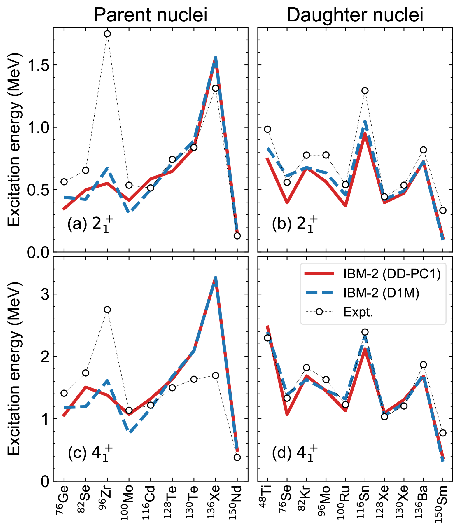
Figure 2: Energy spectra of the $2^{+}_{1}$ and $4^{+}_{1}$ states of the parent and daughter even-even nuclei of the $0\nu\beta\beta$ decays, obtained from the mapped IBM-2 calculations that are based on the relativistic DD-PC1 and nonrelativistic Gogny-D1M EDFs. Experimental data are taken from NNDC [36].

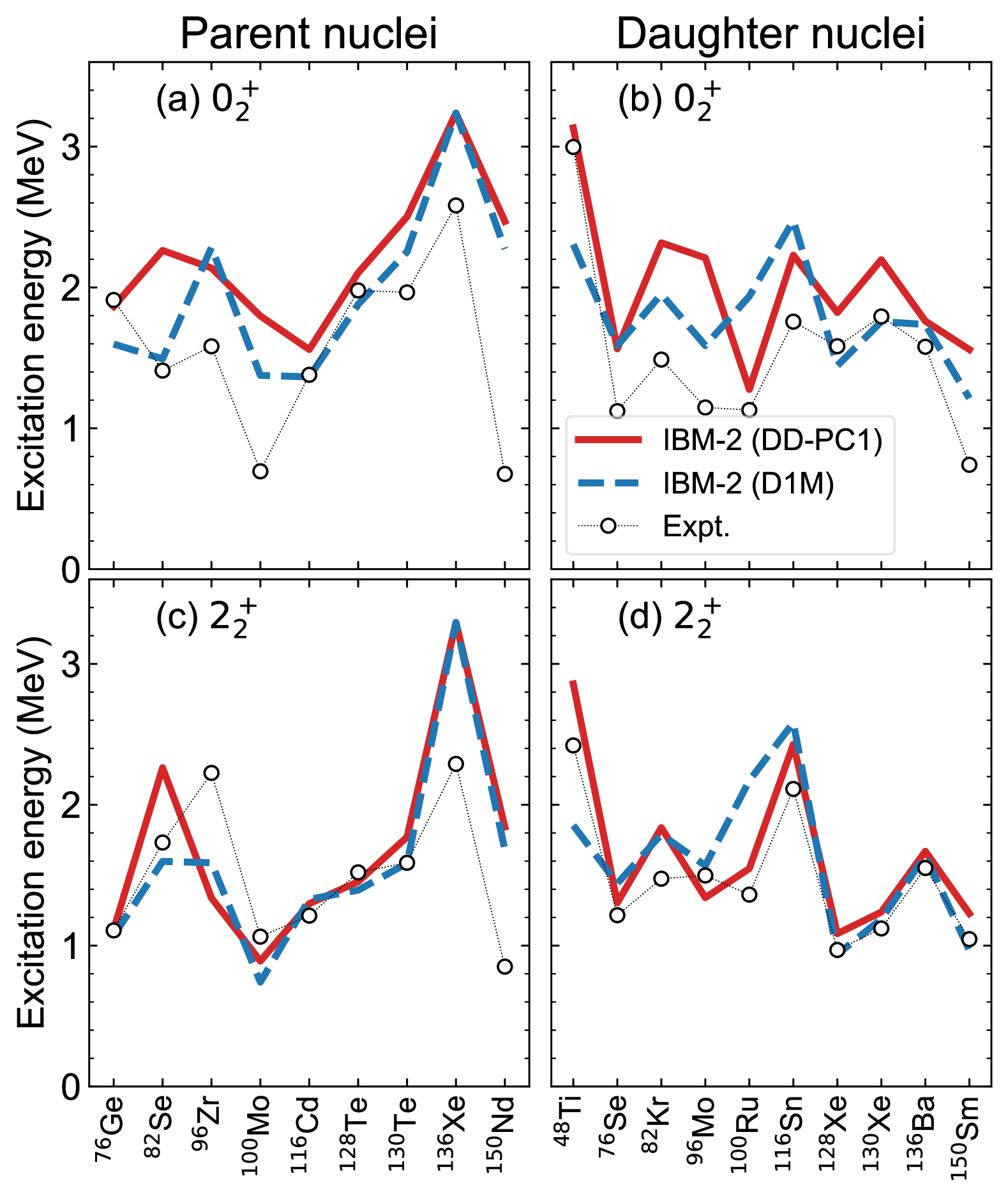
Figure 3: Same as the caption to Fig. 2, but for the $0^{+}_{2}$ and $2^{+}_{2}$ states.

III Low-energy nuclear structures

Figure 1 shows potential energy curves as functions of the axial deformation $\beta$ computed for the even-even nuclei within the RHB and Gogny-D1M HFB methods. The RHB-SCMF triaxial quadrupole $(\beta,\gamma)$ PESs for the studied even-even nuclei are found in Refs. [15, 16]. The Gogny-D1M $(\beta,\gamma)$ PESs for most of the even-even nuclei are found in the previous studies: Ref. [37] for ⁷⁶Ge, ⁷⁶Se and ⁸²Se Ref. [38] for ⁸²Kr, Ref. [39] for ⁹⁶Zr, ⁹⁶Mo, ¹⁰⁰Mo and ¹⁰⁰Ru, Ref. [40] for ¹²⁸Xe, ¹³⁰Xe and ¹³⁶Ba, Ref. [41] for ¹⁵⁰Sm, and Ref. [42] for ¹⁵⁰Nd. The intrinsic properties of these even-even nuclei, including the onset of deformations and shape phase transitions, have been discussed in detail in the above references. It is, therefore, sufficient to consider the PESs along the axial $\beta$ deformation in the present work, which is rather focused on the results on the $0\nu\beta\beta$ decays. The self-consistent PESs with the Gogny-D1M force for the ⁴⁸Ca, ⁴⁸Ti, ¹¹⁶Cd, ¹¹⁶Sn, ¹²⁸Te, ¹³⁰Te and ¹³⁶Xe nuclei are here computed by using the code HFBTHO [43], which assumes the axial symmetry.

Figure 2 gives the excitation energies of the yrast states $2^{+}_{1}$ and $4^{+}_{1}$ of the even-even parent and daughter nuclei computed by the mapped IBM-2 using the relativistic DD-PC1 and nonrelativistic Gogny EDFs. The calculated excitation energies are consistent with the experimental data, except for ⁹⁶Zr and ¹³⁶Xe, for which the calculations considerably underestimate the experimental levels. The nucleus ⁹⁶Zr corresponds to the neutron $N=56$ and proton $Z=40$ subshell closures, and its ground state has indeed been suggested to be spherical in nature experimentally [44]. Both the relativistic and nonrelativistic SCMF calculations for this nucleus rather suggest the PES that exhibits a large prolate or oblate deformation (see Fig. 1) and, consequently, the mapped IBM-2 Hamiltonian produces unexpectedly low-lying $2^{+}_{1}$ and $4^{+}_{1}$ energy levels. Overestimates of the $4^{+}_{1}$ energy encountered for ¹³⁶Xe are due to the fact this nucleus corresponds to the neutron magic number $N=82$, in which case the IBM in general is not quite reliable as it is built only on the valence space.

One can also observe quantitative differences between the IBM-2 spectra obtained from the DD-PC1 and Gogny EDFs. As shown in Fig. 1 the RHB-SCMF PESs generally exhibit a more pronounced deformed minimum or steeper potential valley than those from the Gogny-HFB calculations. The IBM-2 mapping from the DD-PC1 EDF is, therefore, supposed to produce a more rotational-like energy spectrum characterized by the compressed energy levels than in the case of the D1M EDF.

Calculation of the excited $0^{+}$ states is important, since the $\beta\beta$ decay from the ground-state $0^{+}_{1}$ to excited $0^{+}_{2}$ states is also possible. There is indeed experimental evidence for the $0^{+}_{1}$ $\to$ $0^{+}_{2}$ $2\nu\beta\beta$ decays in ¹⁰⁰Mo [45] and ¹⁵⁰Nd (see Ref. [46], and references therein). The mapped IBM-2, particularly when the DD-PC1 force is used, systematically overestimates the $0^{+}_{2}$ energy levels for parent and daughter nuclei. The overestimate of the $0^{+}_{2}$ levels appears to be a general feature of the mapped IBM-2 descriptions, that has been encountered in different mass regions, and can be mainly attributed to the fact that the quadrupole-quadrupole boson interaction strength $\kappa$ derived from the mapping takes a very large negative value, which is by a factor of $\approx$ 2-4 larger than those used in the phenomenological IBM-2 calculations. With the large negative $\kappa$ values, the $d$-boson contributions to low-lying states are appreciably large, and lead to a rotational-like level structure, in which the energy levels in the ground-state band are somewhat compressed and the $0^{+}_{2}$ energy level appears at relatively high energy. The value of the derived $\kappa$ parameter also reflects the features of the SCMF PES. In particular, the potential valley of the PES computed by the SCMF method with many of the relativistic and nonrelativistic EDFs appears to be often quite steep in both $\beta$ and $\gamma$ deformations. In order to reproduce such a feature, the mapping procedure requires to choose the large $|\kappa|$ values. The calculated energy levels, particularly those of the non-yrast states, depend on the feature of the corresponding PES. The DD-PC1 and D1M PESs indeed exhibit different topology in many cases (see Fig. 1). The Gogny-HFB mapped IBM-2 appears to give a lower $0^{+}_{2}$ excitation energy than the RHB-mapped one (see Fig. 3).

In addition, in a few transitional nuclei, e.g., ¹⁰⁰Mo, the observed $0^{+}_{2}$ energy levels are considerably low [see Figs. 3(a) and 3(b)]. These extremely low-lying $0^{+}_{2}$ states may be attributed to the intruder particle-hole excitations, and cannot be reproduced by the standard IBM-2. The effects of the intruder states could be accounted for in the IBM-2 by extending it to include configuration mixing [47, 48, 39].

The level structure of the $\gamma$-soft systems is characterized by the low-lying $2^{+}_{2}$ state close in energy to the ground-state yrast band, and this state is often interpreted as the bandhead of the $\gamma$-vibrational band. In most cases, the mapped IBM-2 results shown in Figs. 3(c) and 3(d) are consistent with the experimental $2^{+}_{2}$ levels, particularly for the daughter nuclei. Certain deviations from the data in ⁹⁶Zr and ¹³⁶Xe occur, because the IBM-2 does not properly account for the (sub-)shell closure effects in these nuclei.

IV $0\nu\beta\beta$ decay

Table 1: Predicted $M_{\mathrm{GT}}^{(0\nu)}$, $M_{\mathrm{F}}^{(0\nu)}$ and $M_{\mathrm{T}}^{(0\nu)}$ matrix elements, and total NME $M^{(0\nu)}$ for the $0^{+}_{1}\to 0^{+}_{1}$ $0\nu\beta\beta$ decays within the mapped IBM-2 based on the DD-PC1 and Gogny-D1M EDFs.

Decay	DD-PC1				D1M
	$M_{\mathrm{GT}}^{(0\nu)}$	$M_{\mathrm{F}}^{(0\nu)}$	$M_{\mathrm{T}}^{(0\nu)}$	$M^{(0\nu)}$	$M_{\mathrm{GT}}^{(0\nu)}$	$M_{\mathrm{F}}^{(0\nu)}$	$M_{\mathrm{T}}^{(0\nu)}$	$M^{(0\nu)}$
48Ca $\to$ 48Ti	$0.713$	$-0.035$	$-0.075$	$0.659$	$1.760$	$-0.062$	$-0.081$	$1.717$
76Ge $\to$ 76Se	$2.801$	$-0.107$	$-0.061$	$2.806$	$4.066$	$-0.163$	$-0.123$	$4.045$
82Se $\to$ 82Kr	$2.136$	$-0.089$	$-0.062$	$2.130$	$2.687$	$-0.113$	$-0.094$	$2.664$
96Zr $\to$ 96Mo	$3.258$	$-0.419$	$0.143$	$3.662$	$3.636$	$-0.558$	$0.141$	$4.123$
100Mo $\to$ 100Ru	$2.732$	$-0.263$	$0.143$	$3.038$	$3.490$	$-0.439$	$0.157$	$3.920$
116Cd $\to$ 116Sn	$3.379$	$-0.564$	$0.130$	$3.859$	$3.479$	$-0.549$	$0.138$	$3.958$
128Te $\to$ 128Xe	$1.671$	$-0.087$	$-0.024$	$1.702$	$2.986$	$-0.161$	$-0.060$	$3.026$
130Te $\to$ 130Xe	$1.474$	$-0.076$	$-0.019$	$1.502$	$3.016$	$-0.163$	$-0.063$	$3.055$
136Xe $\to$ 136Ba	$2.082$	$-0.113$	$-0.047$	$2.106$	$2.545$	$-0.139$	$-0.061$	$2.570$
150Nd $\to$ 150Sm	$4.262$	$-0.844$	$0.142$	$4.929$	$4.078$	$-0.923$	$0.111$	$4.762$

Table 2: Same as Table 1, but for the $0^{+}_{1}\to 0^{+}_{2}$ $0\nu\beta\beta$ decays.

Decay	DD-PC1				D1M
	$M_{\mathrm{GT}}^{(0\nu)}$	$M_{\mathrm{F}}^{(0\nu)}$	$M_{\mathrm{T}}^{(0\nu)}$	$M^{(0\nu)}$	$M_{\mathrm{GT}}^{(0\nu)}$	$M_{\mathrm{F}}^{(0\nu)}$	$M_{\mathrm{T}}^{(0\nu)}$	$M^{(0\nu)}$
48Ca $\to$ 48Ti	$2.743$	$-0.086$	$-0.051$	$2.745$	$2.430$	$-0.067$	$-0.012$	$2.460$
76Ge $\to$ 76Se	$1.300$	$-0.054$	$-0.053$	$1.280$	$0.314$	$-0.016$	$-0.037$	$0.286$
82Se $\to$ 82Kr	$0.584$	$-0.021$	$-0.040$	$0.557$	$0.742$	$-0.028$	$-0.047$	$0.712$
96Zr $\to$ 96Mo	$0.250$	$-0.033$	$0.011$	$0.281$	$0.347$	$-0.052$	$0.014$	$0.393$
100Mo $\to$ 100Ru	$0.093$	$-0.011$	$0.004$	$0.104$	$0.978$	$-0.125$	$0.043$	$1.099$
116Cd $\to$ 116Sn	$0.607$	$-0.104$	$0.017$	$0.689$	$0.488$	$-0.069$	$0.015$	$0.545$
128Te $\to$ 128Xe	$0.139$	$-0.007$	$-0.003$	$0.141$	$0.934$	$-0.050$	$-0.022$	$0.943$
130Te $\to$ 130Xe	$1.018$	$-0.055$	$-0.025$	$1.026$	$2.649$	$-0.142$	$-0.067$	$2.671$
136Xe $\to$ 136Ba	$1.477$	$-0.078$	$-0.043$	$1.483$	$2.002$	$-0.105$	$-0.056$	$2.010$
150Nd $\to$ 150Sm	$0.748$	$-0.089$	$0.026$	$0.829$	$0.441$	$-0.073$	$0.007$	$0.494$

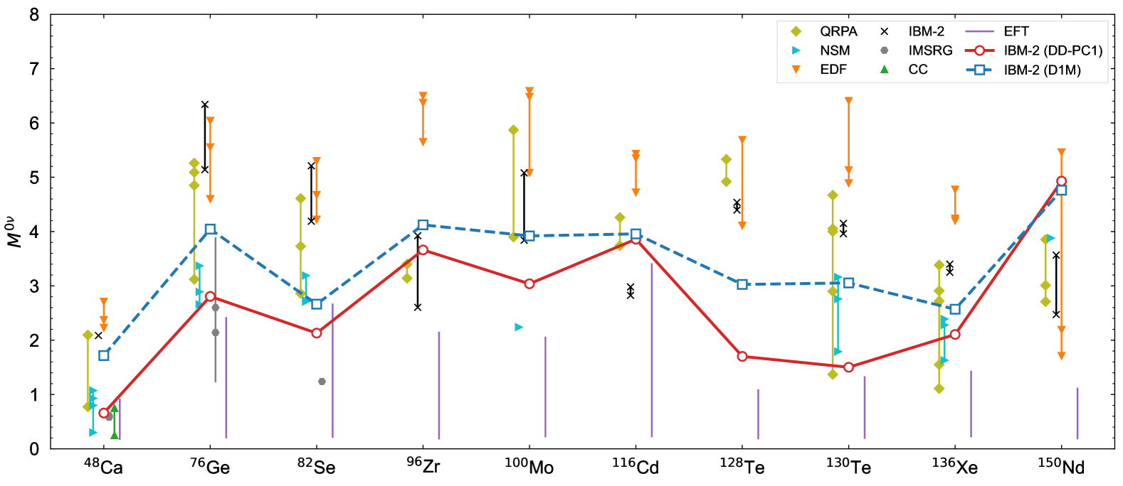
Figure 4: $0\nu\beta\beta$-decay NMEs predicted by the mapped IBM-2 using the relativistic, DD-PC1, and nonrelativistic, Gogny D1M, EDFs. Theoretical predictions within the QRPA [49, 50, 51, 52, 53], NSM [54, 55, 56, 57, 58], EDF-GCM [59, 60, 61], IBM-2 [9, 10], In-Medium Similarity Renormalization Group (IMSRG) approach [62, 63, 64], Coupled Cluster (CC) theory [65], and Effective Field Theory (EFT) [66] are also shown.

Predicted $M_{\mathrm{GT}}^{(0\nu)}$, $M_{\mathrm{F}}^{(0\nu)}$ and $M_{\mathrm{T}}^{(0\nu)}$ matrix elements, and final NMEs $M^{(0\nu)}$ for the $0^{+}_{1}\to 0^{+}_{1}$ decays for the studied $0\nu\beta\beta$ emitters are shown in Table 1. Two sets of the results shown in the table correspond to the calculations employing the relativistic DD-PC1 and nonrelativistic Gogny D1M energy functionals in the self-consistent calculations. The dominant contributions to the total NMEs $M^{(0\nu)}$ are from the GT transitions, while the Fermi and tensor parts appear to play less significant roles. In addition, the NMEs from the Gogny EDFs are generally larger than those from the DD-PC1 EDF.

The NMEs for the $0^{+}_{1}$ $\to$ $0^{+}_{2}$ $0\nu\beta\beta$ decays are also computed with the mapped IBM-2, and appear to depend on the choice of the EDF (see Table 2). The $0^{+}_{1}$ $\to$ $0^{+}_{2}$ decay rates are particularly sensitive to the description of the $0^{+}_{2}$ states of the final nuclei, since the predicted $0^{+}_{2}$ energy levels for the daughter nuclei depend largely on the EDFs [see Fig. 3(b)]. In addition, the coexistence of more than one minimum observed in the PESs for several nuclei should have certain influence on the ground and excited $0^{+}$ states. For ⁹⁶Zr, for instance, both the Gogny-HFB and RHB SCMF calculations suggest two minima that are quite close in energy to each other [39, 15, 16]. In such systems, substantial shape mixing is supposed to occur in the IBM-2 lowest-lying $0^{+}$ states. A possible effect of the coexisting mean-field minima is discussed in Sec. V.2.

Figure 4 displays the calculated $0^{+}_{1}$ $\to$ $0^{+}_{1}$ $0\nu\beta\beta$-decay NMEs, which are also shown in Table 1, and those NMEs values computed by the QRPA [49, 52, 50, 51, 53], NSM [54, 55, 56, 57, 58], EDF-GCM [59, 60, 61], IBM-2 [9, 10], In-Medium Similarity Renormalization Group (IMSRG) approach [62, 63, 64], Coupled Cluster (CC) theory [65], and Effective Field Theory (EFT) [66]. The mapped IBM-2 NMEs for the ⁴⁸Ca decay are small, $M^{(0\nu)}<1$, when the DD-PC1 functional is employed, and are close to the values obtained from the NSM calculations. The D1M-mapped calculation gives a larger NME for the ⁴⁸Ca decay, being rather close to the earlier IBM-2 value [9]. The difference between the two EDF results emerges, probably because the present HFB calculation suggests a spherical minimum for the ⁴⁸Ti, whereas the DD-PC1 SCMF PES predicts a deformed minimum at $\beta\approx 0.15$ (see Fig. 1). For the ⁷⁶Ge $\to$ ⁷⁶Se decay, the RHB-mapped IBM-2 calculation gives a NME that is more or less close to the predictions from the IMSRG [63, 64]. The Gogny-EDF mapped IBM-2, however, produces a much larger NME, being closer to the QRPA values. The mapped IBM-2 NMEs for the ⁸²Se $\to$ ⁸²Kr decay are smaller than many of the calculated NMEs in the EDF, QRPA, NSM, and IBM-2, but are close to the IMSRG [63] and EFT [66] values. For both the ⁷⁶Ge $\to$ ⁷⁶Se and ⁸²Se $\to$ ⁸²Kr decays, the mapped IBM-2 NMEs are approximately by a factor of 2 lower than those of the previous IBM-2 calculations [9, 10].

For the ⁹⁶Zr $\to$ ⁹⁶Mo, ¹⁰⁰Mo $\to$ ¹⁰⁰Ru, and ¹¹⁶Cd $\to$ ¹¹⁶Sn decays, the EDF-mapped IBM-2 yields the NMEs that are more or less close to the IBM-2 values of Refs. [9, 10]. The present values of the NMEs for the ¹²⁸Te $\to$ ¹²⁸Xe and ¹³⁰Te $\to$ ¹³⁰Xe decays are systematically smaller than those in the majority of the other model calculations. The DD-PC1 and D1M mapped IBM-2 NMEs also differ from each other for the above two decay processes. For the ¹³⁶Xe $\to$ ¹³⁶Ba $0\nu\beta\beta$ decay, the two EDF-mapped IBM-2 calculations provide the NME values close to those from other approaches. In contrast to all the other $0\nu\beta\beta$-decay processes, the present NME values for the ¹⁵⁰Nd $\to$ ¹⁵⁰Sm decay appear to be among the largest of the NME values found in the literature.

Figure 5: Decomposition of the GT matrix elements into the monopole ($J=0$) and quadrupole ($J=2$) components.

To give further insights into the nature of the calculated NMEs, the GT matrix element $M_{\mathrm{GT}}^{(0\nu)}$, a dominant factor in the total NME, is decomposed into the monopole and quadrupole components, which correspond to the first and second terms in Eq. (II.2), respectively. For the $0^{+}_{1}$ $\to$ $0^{+}_{1}$ $0\nu\beta\beta$-decay processes, the monopole contribution is dominant over the quadrupole one, as shown in Fig. 5. In general, larger monopole contributions are obtained when the Gogny-D1M interaction is adopted as a microscopic basis than in the case of the relativistic DD-PC1 interaction. There is no notable difference between the quadrupole components of $M_{\mathrm{GT}}^{(0\nu)}$ obtained from both EDF interactions, except for the ⁴⁸Ca decay. The ratios of the quadrupole to monopole GT matrix elements calculated with the DD-PC1 force are, therefore, systematically larger than those with the D1M force. For the ⁴⁸Ca, ¹²⁸Te and ¹³⁰Te $0\nu\beta\beta$ decays, the quadrupole-to-monopole ratios amount to 59 %, 43 %, and 46 %, respectively, in the case of the DD-PC1 input. In the calculations with the Gogny-D1M force, these ratios are less than 30 % for all the studied $0\nu\beta\beta$-decay processes.

Table 3: Predicted half-lives $T_{1/2}^{(0\nu\beta\beta)}$ (in yr) for the $0^{+}_{1}\to 0^{+}_{1}$ $0\nu\beta\beta$ decays within the EDF-mapped IBM-2 assuming the average light neutrino mass of $\braket{m_{\nu}}=1$ eV. The results obtained with the microscopic inputs from the relativistic DD-PC1 (column 2), and nonrelativistic Gogny D1M (column 4) EDFs are shown. In columns 3 and 5 shown are the upper limits of the neutrino mass estimated using the 90 % C.L. limits on $T_{1/2}^{(0\nu\beta\beta)}$’s, adopted from the complication of [5] (column 6).

Decay	DD-PC1		D1M		$T_{1/2,{\rm expt}}^{(0\nu\beta\beta)}$ (yr)
	$T_{1/2}^{(0\nu\beta\beta)}$ (yr)	$\braket{m_{\nu}}$ (eV)	$T_{1/2}^{(0\nu\beta\beta)}$ (yr)	$\braket{m_{\nu}}$ (eV)
48Ca $\to$ 48Ti	$9.34\times 10^{24}$	$<12.690$	$1.38\times 10^{24}$	$<4.860$	$>5.8\times 10^{22}$
76Ge $\to$ 76Se	$5.41\times 10^{24}$	$<0.173$	$2.60\times 10^{24}$	$<0.120$	$>1.8\times 10^{26}$
82Se $\to$ 82Kr	$2.18\times 10^{24}$	$<0.789$	$1.40\times 10^{24}$	$<0.630$	$>4.6\times 10^{24}$
96Zr $\to$ 96Mo	$3.65\times 10^{23}$	$<6.255$	$2.88\times 10^{23}$	$<5.517$	$>9.2\times 10^{21}$
100Mo $\to$ 100Ru	$6.85\times 10^{23}$	$<0.673$	$4.12\times 10^{23}$	$<0.516$	$>1.8\times 10^{24}$
116Cd $\to$ 116Sn	$4.05\times 10^{23}$	$<1.348$	$3.85\times 10^{23}$	$<1.314$	$>2.2\times 10^{23}$
128Te $\to$ 128Xe	$5.92\times 10^{25}$	$<6.280$	$1.87\times 10^{25}$	$<3.531$	$>3.6\times 10^{24}$
130Te $\to$ 130Xe	$3.14\times 10^{24}$	$<0.377$	$7.59\times 10^{23}$	$<0.185$	$>2.2\times 10^{25}$
136Xe $\to$ 136Ba	$1.56\times 10^{24}$	$<0.375$	$1.05\times 10^{24}$	$<0.307$	$>2.3\times 10^{26}$
150Nd $\to$ 150Sm	$6.58\times 10^{22}$	$<1.732$	$7.04\times 10^{22}$	$<1.732$	$>2.0\times 10^{22}$

Table 3 gives the half-lives for the $0^{+}_{1}\to 0^{+}_{1}$ $0\nu\beta\beta$ decays (7), computed by using the NMEs shown in Table 1 and Fig. 4. The phase-space factors $G_{0\nu}$ are adopted from Ref. [67], and the average light neutrino mass of $\braket{m_{\nu}}=1$ eV is assumed. The upper limits of $\braket{m_{\nu}}$ estimated by using the current limits on the $T_{1/2}^{(0\nu\beta\beta)}$, adopted from the recent compilation of Gómez-Cadenas et al. [5], are also shown in Table 1, and it appears that the Gogny-mapped IBM-2 overall gives shorter $T_{1/2}^{(0\nu\beta\beta)}$, hence slightly more stringent limits on neutrino mass, than the RHB-mapped IBM-2 calculation.

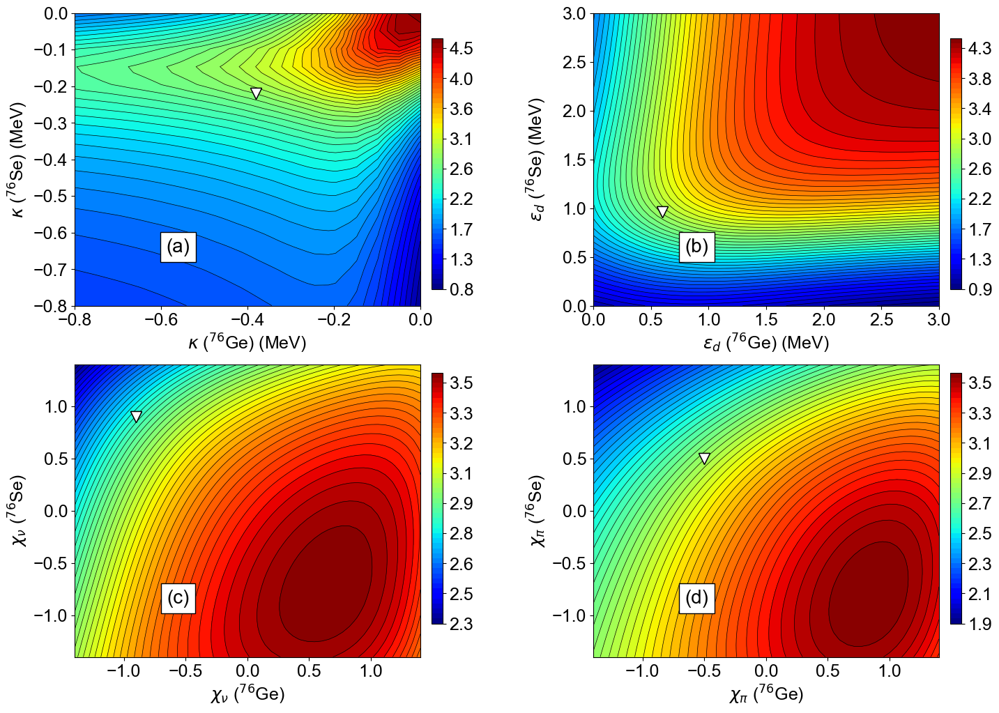
Figure 6: Calculated NMEs for the $0\nu\beta\beta$ decay ⁷⁶Ge$(0^{+}_{1})$ $\to$ ⁷⁶Se$(0^{+}_{1})$ as functions of the parameters (a) $\kappa$, (b) $\epsilon$, (c) $\chi_{\nu}$, and (d) $\chi_{\pi}$ for the parent and daughter nuclei. The microscopic input for the IBM-2 mapping is the DD-PC1 EDF. The open triangle indicates the NME values calculated with the sets of the parameters obtained from the mapping.

V Sensitivity analyses

The predicted NME values appear to be sensitive to the parameters and assumptions considered in the calculations. In particular, it has been shown in preceding sections that the choice of the EDF considerably affects the energy spectra (Figs. 2 and 3) and $0\nu\beta\beta$-decay NMEs (Fig. 4). In the present section, dependencies of the mapped IBM-2 NME results on the strength parameters of the IBM-2 Hamiltonian, on the coexistence of mean-field minima in the SCMF PESs that appears in some nuclei, and on the pair structure constants for the $0\nu\beta\beta$ transition operators are discussed.

V.1 IBM-2 Hamiltonian parameters

Even though the IBM-2 Hamiltonian parameters are specified by the mapping procedure, it is of interest to analyze dependencies of the calculated NMEs on these parameters. Figure 6 shows contour plots of the NMEs for the decay ⁷⁶Ge$(0^{+}_{1})$ $\to$ ⁷⁶Se$(0^{+}_{1})$ in terms of the IBM-2 Hamiltonian parameters for the parent and daughter nuclei. The behaviors of the NMEs with the changes in the parameters are similar to those for the other $0\nu\beta\beta$-decay processes considered in the present work. Also in this analysis, only one of the parameters for each even-even nucleus is varied, keeping all the other parameters unchanged, and the cubic term is not considered for simplicity.

The quadrupole-quadrupole strength $\kappa$ is expected to influence significantly the spectroscopic properties of each nucleus and the NMEs, since the term $\hat{Q}_{\nu}\cdot\hat{Q}_{\pi}$ is most responsible for determining the $d$-boson contents in the wave functions for the ground and excited $0^{+}$ states. The relevance of the quadrupole-quadrupole strength $\kappa$ was investigated in the studies of the $2\nu\beta\beta$ decays [16] and single-$\beta$ decay properties of the neutron-rich Zr isotopes [68]. It was shown in [16] that the decrease in magnitude of this parameter led to the enhancement of the $2\nu\beta\beta$-decay NMEs [16]. The parameter sensitivity analysis for the mapped IBM-2 in Ref. [68] suggested that by decreasing the magnitude $|\kappa|$ the calculated $\beta$-decay $\log(ft)$ values of the neutron-rich Zr isotopes became larger and consistent with data [68]. With the decreases in magnitude of the quadrupole-quadrupole strengths $\kappa$ for the parent (⁷⁶Ge) and daughter (⁷⁶Se) nuclei, the NME becomes larger [Fig. 6(a)]. These behaviors of the NME are explained by the fact that the $d$-boson contributions are suppressed by the decreases in the magnitude $|\kappa|$, while the dominant, monopole components in the NME are enhanced.

As shown in Fig. 6(b), larger values of the NMEs are obtained by increasing the single $d$-boson energies $\epsilon_{d}$, since the monopole contributions become even more dominant over the quadrupole ones. The NMEs appear to be less sensitive to the changes in the parameters $\chi_{\nu}$ [Fig. 6(c)] and $\chi_{\pi}$ [Fig. 6(d)] than to $\kappa$ and $\epsilon_{d}$. In Fig. 6(c), largest NMEs are obtained if the values $\chi_{\nu}\approx$ 0.5 and $-0.5$ are taken for ⁷⁶Ge and ⁷⁶Se, respectively. These $\chi_{\nu}$ values are opposite in sign, but in the same of order of magnitude as the $\chi_{\pi}$ parameter values determined by the mapping, that is, $\chi_{\pi}=-0.5$ and 0.5 for ⁷⁶Ge and ⁷⁶Se, respectively. The sum $\chi_{\nu}+\chi_{\pi}$ that nearly vanishes indicates that the quadrupole deformation is significantly suppressed, since assuming that the quadrupole operator for the total boson system is approximately given as $\hat{Q}_{\nu}+\hat{Q}_{\pi}$ the matrix element of the term $\chi_{\nu}(d^{\dagger}_{\nu}\times\tilde{d}_{\nu})^{(2)}+\chi_{\pi}(d^{\dagger}_{\pi}\times\tilde{d}_{\pi})^{(2)}$ is significantly reduced. The monopole components are, however, supposed to play an even more significant role and produce the enhanced NMEs, with the above combination of the $\chi_{\nu}$ and $\chi_{\pi}$ values. Also in Fig. 6(d) the $\chi_{\pi}$ values of $\chi_{\pi}\approx$ 0.9 (⁷⁶Ge) and $-0.9$ (⁷⁶Se) give the largest NMEs, and these values are in the same order of magnitude as the derived $\chi_{\nu}$ values, $-0.9$ (⁷⁶Ge) and 0.9 (⁷⁶Se).

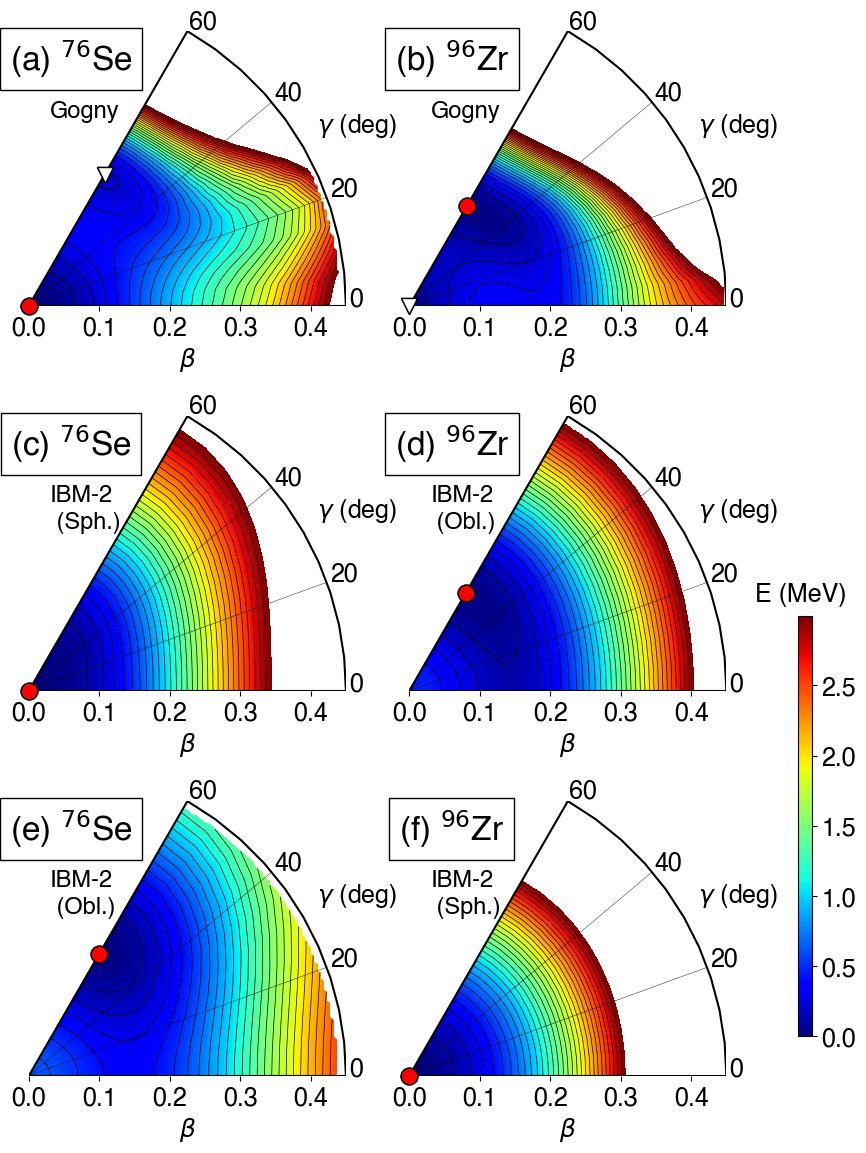
Figure 7: SCMF PESs in terms of the triaxial quadrupole $(\beta,\gamma)$ deformations for (a) ⁷⁶Se and (b) ⁹⁶Zr, computed by the constrained HFB method based on the Gogny D1M EDF, the corresponding IBM-2 PESs with the Hamiltonian associated with the global [(c) and (d)], and local [(e) and (f)] minima on the SCMF PESs. The global, and local minima on the Gogny-HFB PESs are denoted by the solid circle and open triangle, respectively. The minimum on the IBM-2 PESs is indicated by the solid circle.

V.2 Coexistence of more than one mean-field minimum

In those nuclei for which the PESs exhibit a local minimum close in energy to the global minimum, there supposed to be certain shape mixing, which influences the spectroscopic properties and NME calculations. The effects of coexisting minima are here analyzed by performing two sets of the mapped IBM-2 calculations, one in which the Hamiltonian is associated with the global minimum, and the other in which the Hamiltonian is associated with a local minimum.

As illustrative cases the Gogny-D1M mapped IBM-2 calculations for the decays ⁷⁶Ge$(0^{+}_{1})$ $\to$ ⁷⁶Se$(0^{+}_{1,2})$ and ⁹⁶Zr$(0^{+}_{1})$ $\to$ ⁹⁶Mo$(0^{+}_{1,2})$ are considered. The Gogny-D1M PESs for ⁷⁶Se and ⁹⁶Zr are given in Fig. 7, and one can see an oblate local minimum for ⁷⁶Se and a spherical local minimum for ⁹⁶Zr. The derived parameters for the ⁷⁶Se from the mapping that is based on the spherical local (oblate global) minimum are $\epsilon_{d}=0.8$ (1.0) MeV, $\kappa=-0.2$ ($-0.14$) MeV, $\chi_{\nu}=0.4$ (0.4), and $\chi_{\pi}=0.4$ (0.4). For the ⁹⁶Zr nucleus, $\epsilon_{d}=1.8$ (1.24) MeV, $\kappa=-0.18$ ($-0.25$) MeV, $\chi_{\nu}=-0.25$ ($-0.25$), and $\chi_{\pi}=0.47$ (0.47), which are derived from the mapping procedure using the oblate local (spherical global) minimum.

Table 4: GT, Fermi, tensor, and total nuclear matrix elements for ⁷⁶Ge$(0^{+}_{1})$ $\to$ ⁷⁶Se$(0^{+}_{1})$ and ⁹⁶Zr$(0^{+}_{1})$ $\to$ ⁹⁶Mo$(0^{+}_{1})$ $0\nu\beta\beta$ decays calculated by the Gogny-D1M mapped IBM-2, with the Hamiltonian associated with the global and local minima. The mean-field minima are found on spherical (“Sph.”) and oblate (“Obl.”) configurations, and that configuration corresponding to the global minimum is shown in bold font.

Decay	config.	$M_{\mathrm{GT}}^{(0\nu)}$	$M_{\mathrm{F}}^{(0\nu)}$	$M_{\mathrm{T}}^{(0\nu)}$	$M^{(0\nu)}$
76Ge $\to$ 76Se	Sph. (76Se)	$4.066$	$-0.163$	$-0.123$	$4.045$
	Obl. (76Se)	$3.631$	$-0.144$	$-0.096$	$3.625$
96Zr $\to$ 96Mo	Sph. (96Zr)	$4.303$	$-0.687$	$0.156$	$4.885$
	Obl. (96Zr)	$3.636$	$-0.558$	$0.141$	$4.123$

Table 5: Same as the caption to Table 5, but for the $0^{+}_{1}$ $\to$ $0^{+}_{2}$ decays.

Decay	config.	$M_{\mathrm{GT}}^{(0\nu)}$	$M_{\mathrm{F}}^{(0\nu)}$	$M_{\mathrm{T}}^{(0\nu)}$	$M^{(0\nu)}$
76Ge $\to$ 76Se	Sph. (76Se)	$0.314$	$-0.016$	$-0.037$	$0.286$
	Obl. (76Se)	$1.833$	$-0.077$	$-0.078$	$1.802$
96Zr $\to$ 96Mo	Sph. (96Zr)	$0.781$	$-0.126$	$0.028$	$0.887$
	Obl. (96Zr)	$0.347$	$-0.052$	$0.014$	$0.393$

Table 6: Monopole ($J=0$) and quadrupole ($J=2$) parts of the GT matrix elements $M_{\mathrm{GT}}^{(0\nu)}$ for the $0\nu\beta\beta$ decays ⁷⁶Ge$(0^{+}_{1})$ $\to$ ⁷⁶Se$(0^{+}_{1,2})$ and ⁹⁶Zr$(0^{+}_{1})$ $\to$ ⁹⁶Mo$(0^{+}_{1,2})$. That configuration corresponding to the global minimum on the SCMF PES is indicated in bold font.

Decay	Config.	$0^{+}_{1}\to 0^{+}_{1}$		$0^{+}_{1}\to 0^{+}_{2}$
		$J=0$	$J=2$	$J=0$	$J=2$
76Ge $\to$ 76Se	Sph. (76Se)	$4.230$	$-0.164$	$0.101$	$0.212$
	Obl. (76Se)	$3.888$	$-0.257$	$1.726$	$0.107$
96Zr $\to$ 96Mo	Sph. (96Zr)	$4.529$	$-0.226$	$0.814$	$-0.033$
	Obl. (96Zr)	$4.032$	$-0.396$	$-0.398$	$0.051$

The resultant NMEs are given in Table 4 and Table 5 for the $0^{+}_{1}$ $\to$ $0^{+}_{1}$ and $0^{+}_{1}$ $\to$ $0^{+}_{2}$ decays, respectively. For the ⁷⁶Ge $\to$ ⁷⁶Se decay, the IBM-2 mapping calculation based on the oblate local minimum in ⁷⁶Se provides the GT, Fermi and tensor matrix elements for the $0^{+}_{1}\to 0^{+}_{1}$ decay that are smaller in magnitude than those based on the spherical global minimum, and gives the final NME that is by approximately 23 % smaller than that obtained with the spherical configuration (see Table 4). Also for the ⁹⁶Zr$(0^{+}_{1})\to^{96}$Mo$(0^{+}_{1})$ decay, the mapped IBM-2 based on the spherical local minimum in ⁹⁶Zr, gives a larger NME than the calculation based on the deformed oblate global minimum.

As seen in Table 5, the NMEs for the $0^{+}_{1}\to 0^{+}_{2}$ decays depend strongly on whether the mapping is carried out at the spherical or deformed mean-field minimum. Indeed, the mapped IBM-2 NME for the ⁷⁶Ge$(0^{+}_{1})\to^{76}$Se$(0^{+}_{2})$ decay, calculated by using the deformed oblate local minimum, is by a factor of approximately 6 larger than that obtained from the calculation based on the spherical global minimum. However, the calculated ⁹⁶Zr$(0^{+}_{1})\to^{96}$Mo$(0^{+}_{2})$ $0\nu\beta\beta$ decay NME with the oblate deformed configuration is by a factor of approximately 2 smaller than that with the spherical local minimum.

Table 6 gives monopole ($J=0$) and quadrupole ($J=2$) components of the GT matrix elements, $M_{\mathrm{GT}}^{(0\nu)}(J=0)$ and $M_{\mathrm{GT}}^{(0\nu)}(J=2)$, calculated by the IBM-2 corresponding to the global and local minima. For the $0^{+}_{1}$ $\to$ $0^{+}_{1}$ $0\nu\beta\beta$ decays of both ⁷⁶Ge and ⁹⁶Zr, the $M_{\mathrm{GT}}^{(0\nu)}(J=0)$ values resulting from the spherical configuration are larger in magnitude than those from the oblate deformed configuration, while the quadrupole contributions become minor if the mapping is made at the spherical configuration. For the $0^{+}_{1}$ $\to$ $0^{+}_{2}$ decay of ⁷⁶Ge, the calculation based on the oblate deformed configuration results in a larger monopole GT matrix elements than that based on the spherical configuration (see Table 6). The interpretation of the results for this decay process is thus not simple. This finding indicates that significant degrees of shape mixing are supposed to enter the IBM-2 $0^{+}_{2}$ wave functions for ⁷⁶Se. To explicitly take into account the coexisting minima and their mixing, the IBM-2 should be extended to include intruder configurations corresponding to the $2n$-particle-$2n$-hole ($n=1,2,\ldots$) excitations from next major shell and their couplings with the normal configuration [47]. This extension would require a major modification of the present theoretical framework, and is beyond the scope of this study.

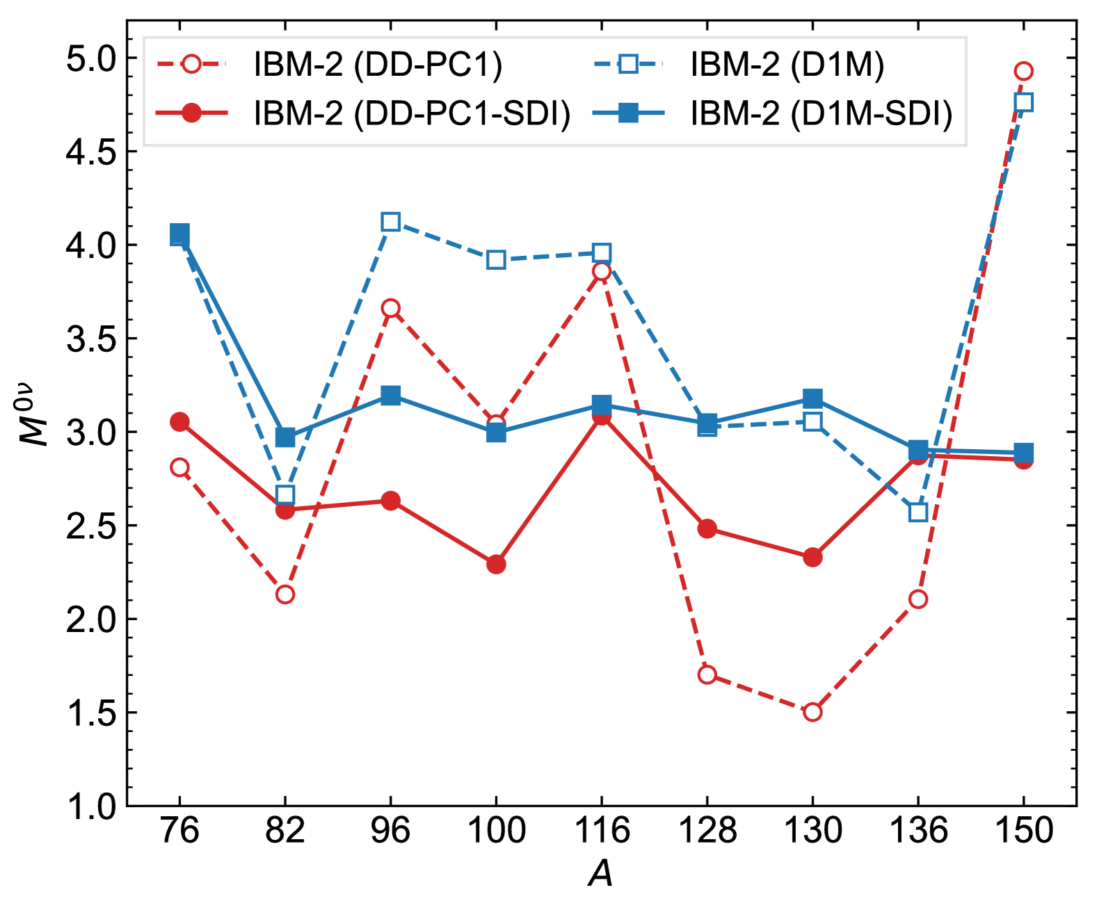
Figure 8: GT matrix elements $M_{\mathrm{GT}}^{(0\nu)}$ computed with the pair structure constants determined by the inputs from the EDF, and with those obtained from the surface-delta interactions (SDIs) of Ref. [7].

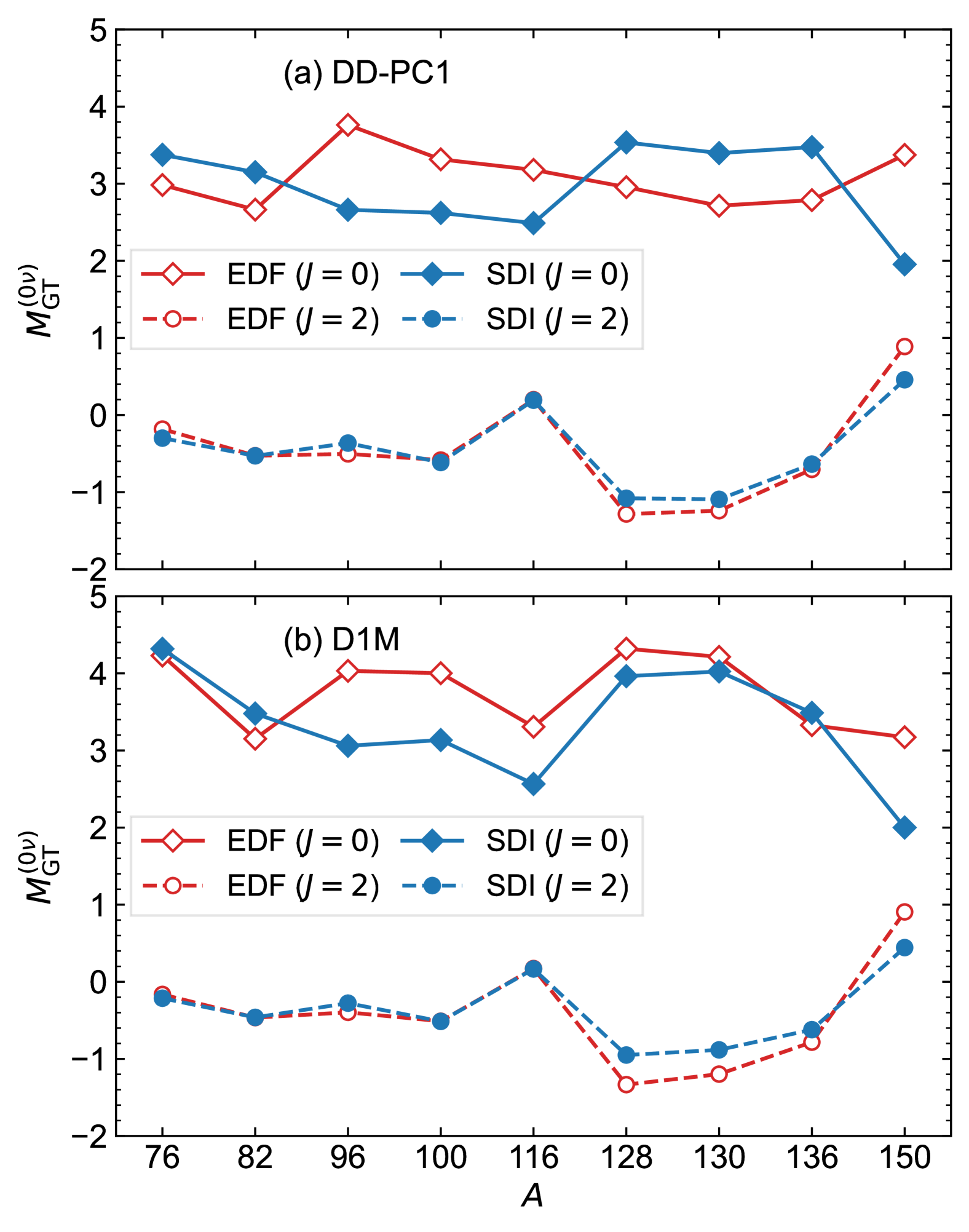
Figure 9: Decomposition of the $M_{\mathrm{GT}}^{(0\nu)}$ into monopole ($J=0$) and quadrupole ($J=2$) components, obtained by using the pair structure constants resulting from the EDF and SDI inputs.

V.3 Pair structure constants

The $0\nu\beta\beta$ NME predictions should depend on the coefficients $\alpha_{j}$ and $\beta_{j_{1}j_{2}}$ in the pair creation operators [Eqs. (21) and (22)], which also appear in the coefficients of the $\beta\beta$ operators, $A_{\rho}(j)$ (70) and $B_{\rho}(j_{1},j_{2})$ (74). In the earlier IBM-2 NME calculations [7, 9], the pair structure constants were obtained from the diagonalization of the shell model Hamiltonian employing the surface delta interactions (SDIs), and the relative sign of $\alpha_{j}$ to $\beta_{j_{1}j_{2}}$ was determined using the formula of Eq. (24). In the present formalism, these parameters are determined in a different way, that is, $\alpha_{j}$ values are calculated for each decay process by using the occupation probabilities $v_{j}^{2}$ [see Eq. (23)] computed with the self-consistent calculations, and $\beta_{j_{1}j_{2}}$ values are calculated by using the formula of (24) (see also the descriptions in Sec. II.2).

Figure 8 shows the NMEs calculated by using the EDF- and SDI-derived pair structure constants. Here the SDIs refer to those shown from Table XIV to Table XVI of Ref. [7], which are denoted as “Set I”, corresponding to different neutron and proton major shells. The $0\nu\beta\beta$-decay NMEs calculated using the SDIs for the decays of ⁷⁶Ge, ⁸²Se, ¹²⁸Te, ¹³⁰Te, and ¹³⁶Xe are larger than those calculated with the EDFs. However, the SDI-based NMEs for the $0\nu\beta\beta$ decays of ⁹⁶Zr, ¹⁰⁰Zr, ¹¹⁶Cd, and ¹⁵⁰Nd are smaller than those based on the EDFs.

Figure 9 depicts decomposition of the $M_{\mathrm{GT}}^{(0\nu)}$ matrix elements into monopole and quadrupole components. It is seen that the monopole parts substantially differ between the calculations employing the EDF- and SDI-derived pair structure constants, while the quadrupole parts are not sensitive to the values of these constants, except for the ¹²⁸Te, ¹³⁰Te, and ¹⁵⁰Nd decays when the DD-PC1 EDF is employed. The monopole components of the NMEs depend only on the $\alpha_{j}$ parameters [see (70)], and therefore the following discussion concerns sensitivity of the NME results to the $\alpha_{j}$ values.

As illustrative examples, Tables 7 and 8 give the neutron and proton pair structure constants $\alpha_{j}$ used to compute the NMEs of the decays ¹³⁰Te $\to$ ¹³⁰Xe and ¹⁵⁰Nd $\to$ ¹⁵⁰Sm, respectively. As shown in Fig. 9, the $M_{\mathrm{GT}}^{(0\nu)}$ values for the ¹³⁰Te (¹⁵⁰Nd) decay obtained from the EDF inputs are smaller (larger) than that calculated by using the pair structure constants computed using the SDIs. Tables 7 and 8 also show the quantity in percent

$$\Delta\alpha_{j}=\frac{\alpha_{j}^{\rm(EDF)}-\alpha_{j}^{\rm(SDI)}}{\alpha_{j}^{\rm(SDI)}}\;,$$ (30)

which measures the difference between the EDF-based $\alpha_{j}^{\rm(EDF)}$ and SDI-based $\alpha_{j}^{\rm(SDI)}$ values. In Table 7, it is seen that for the ¹³⁰Te decay, in the case of the DD-PC1 input $\alpha_{j}^{\rm(EDF)}$ values are in most cases smaller than the $\alpha_{j}^{\rm(SDI)}$, i.e., $\Delta\alpha_{j}<0$. The $\alpha_{j}^{\rm(EDF)}$ values from the Gogny-D1M input appear to be, however, more or less close to the SDI counterparts. As one can see in Table 8, the $\alpha_{j}^{\rm(EDF)}$ values with both the DD-PC1 and D1M EDF inputs are, in most cases, considerably larger than the $\alpha_{j}^{\rm(SDI)}$ values. The $\nu\alpha_{9/2}$ value for the neutron $h_{9/2}$ orbit obtained from the DD-PC1 EDF, in particular, is by more than a factor of 4 larger than that based on the SDI. These differences between $\alpha_{j}^{\rm(EDF)}$ and $\alpha_{j}^{\rm(SDI)}$ appear to account for the discrepancies between the GT matrix elements obtained from the EDF and SDI inputs, demonstrated in Figs. 8 and 9.

Table 7: Pair structure constants $\alpha_{j}$ for the neutron and proton $3s_{1/2}$, $2d_{3/2}$, $2d_{5/2}$, $1g_{7/2}$, and $1h_{11/2}$ orbits employed for the operators in (II.2) for the $0\nu\beta\beta$ decay of the ¹³⁰Te. Those $\alpha_{j}$ values determined by the occupation probabilities $v^{2}_{j}$ computed with the DD-PC1 and Gogny-D1M EDFs, and those derived from the SDI are shown. The quantity $\Delta\alpha_{j}$ (in %) is defined in Eq. (30). The $\alpha_{j}$ values based on the SDI for neutrons and protons are taken from Table XV of Ref. [7], in which they are denoted as “Neutrons (I) (holes)” and “Protons (particles)”.

Orbit	SDI	DD-PC1		D1M
	$\alpha_{j}$	$\alpha_{j}$	$\Delta\alpha_{j}$ (%)	$\alpha_{j}$	$\Delta\alpha_{j}$ (%)
$\nu s_{1/2}$	$-0.999$	$-0.999$	$0$	$-0.830$	$-17$
$\nu d_{3/2}$	$-1.395$	$-0.847$	$-39$	$-0.927$	$-34$
$\nu d_{5/2}$	$-0.469$	$-0.411$	$-12$	$-0.405$	$-14$
$\nu g_{7/2}$	$-0.357$	$-0.316$	$-11$	$-0.453$	$27$
$\nu h_{11/2}$	$1.287$	$1.453$	$13$	$1.431$	$11$
$\pi s_{1/2}$	$0.382$	$0.226$	$-41$	$0.379$	$-1$
$\pi d_{3/2}$	$0.414$	$0.320$	$-23$	$0.509$	$23$
$\pi d_{5/2}$	$0.817$	$0.581$	$-29$	$1.154$	$41$
$\pi g_{7/2}$	$1.769$	$1.879$	$6$	$1.602$	$-9$
$\pi h_{11/2}$	$-0.406$	$-0.320$	$-21$	$-0.424$	$4$

Table 8: Same as 7, but for the $\alpha_{j}$ values for the neutron $3p_{1/2}$, $3p_{3/2}$, $2f_{5/2}$, $2f_{7/2}$, $1h_{9/2}$, and $1i_{13/2}$ orbits, and proton $3s_{1/2}$, $2d_{3/2}$, $2d_{5/2}$, $1g_{7/2}$, and $1h_{11/2}$ orbits used for the ¹⁵⁰Nd decay. The $\alpha_{j}$ values based on the SDI for neutrons are taken from Table XVI of Ref. [7], in which they are denoted as “Neutrons (I)”, and those values for protons are adopted from Table XV in the same reference, denoted as “Protons”.

Orbit	SDI	DD-PC1		D1M
	$\alpha_{j}$	$\alpha_{j}$	$\Delta\alpha_{j}$ (%)	$\alpha_{j}$	$\Delta\alpha_{j}$ (%)
$\nu p_{1/2}$	$-0.418$	$-0.275$	$-34$	$-0.373$	$-11$
$\nu p_{3/2}$	$-0.572$	$-0.318$	$-44$	$-0.507$	$-11$
$\nu f_{5/2}$	$-0.371$	$-0.451$	$22$	$-0.509$	$37$
$\nu f_{7/2}$	$-2.188$	$-1.070$	$-51$	$-1.752$	$-20$
$\nu h_{9/2}$	$-0.390$	$-1.752$	$349$	$-1.141$	$192$
$\nu i_{13/2}$	$0.349$	$0.411$	$18$	$0.506$	$45$
$\pi s_{1/2}$	$0.382$	$0.506$	$32$	$0.627$	$64$
$\pi d_{3/2}$	$0.414$	$0.789$	$90$	$0.779$	$88$
$\pi d_{5/2}$	$0.817$	$1.804$	$121$	$1.505$	$84$
$\pi g_{7/2}$	$1.769$	$0.603$	$-66$	$1.119$	$-37$
$\pi h_{11/2}$	$-0.406$	$-0.740$	$82$	$-0.657$	$62$

VI Concluding remarks

Predictions on the $0\nu\beta\beta$-decay NMEs have been made using the framework of the IBM-2 that is based on the nuclear EDF theory. The IBM-2 Hamiltonian, which yields energies and wave functions of the ground and excited states for $0\nu\beta\beta$ emitting even-even isotopes and corresponding final-state nuclei, has been determined by mapping the self-consistent PES obtained with a given EDF onto the corresponding energy surface in the boson intrinsic state. The GT, Fermi, and tensor transition operators have been formulated by using the generalized seniority scheme, which was also considered in Ref. [7]. The short range correlations for the neutrino potential have been taken into account using the Argonne parametrization. To show the robustness of the predictions, both the relativistic and nonrelativistic EDFs have been employed for the mapping procedure.

The calculated values of the $0\nu\beta\beta$-decay NMEs have been compared to those resulting from different nuclear many-body methods. The present values of the NMEs, in most cases, substantially differ from the earlier IBM-2 predictions [9, 10], which employed the same formulation for the $0\nu\beta\beta$ transitions operators as that in the present study. The differences could be accounted for by the facts that in these previous IBM-2 studies the Hamiltonian parameters were so chosen as to reproduce the experimental low-energy spectra, and that the pair structure constants were calculated using the SDIs in the shell model. The NMEs calculated by the EDF-mapped IBM-2 are more less close to many of the NSM and ab initio values, but are smaller than most of the QRPA and EDF-GCM results. The predicted NMEs have also been shown to depend substantially on the choice of the underlying EDF. The Gogny-D1M mapped IBM-2 appears to yield larger NMEs than the relativistic one.

On the basis of the parameter sensitivity analyses, it appears that certain extensions of the present framework are needed. In particular, the self-consistent calculations suggest a local mean-field minimum that is close in energy to the global minimum, e.g., in ⁷⁶Se and ⁹⁶Zr. In such cases the mean-field configurations associated with the coexisting minima would influence the calculated spectroscopic properties and $0\nu\beta\beta$-decay NMEs. To incorporate the coexisting minima the present framework should be extended to include configuration mixing between normal and intruder states in the IBM-2 space. Other extension of the present framework can be the inclusion of additional interaction terms in the IBM-2 Hamiltonian such as the so-called Majorana interactions, which concern the neutron-proton mixed symmetry and which have been introduced in earlier IBM-2 calculations on the $0\nu\beta\beta$ NMEs [7, 8, 9]. Additional boson degrees of freedom, including the octupole and hexadecapole ones, may have potential impacts on the NMEs. These extensions will be important steps forward in the $0\nu\beta\beta$ NME predictions within the IBM.

Appendix A Details about formulas

A.1 Form factors

Terms that appear in the form factors $\tilde{h}^{\alpha}(p)$ (14)–(16) have the following forms.

$$\tilde{h}^{\rm F}_{VV}(p)=g_{\mathrm{V}}^{2}(p^{2})$$ (31)

$$\tilde{h}^{\rm GT}_{AA}(p)=g_{\mathrm{A}}^{2}(p^{2})$$ (32)

$$\tilde{h}^{\rm GT}_{AP}(p)=-\frac{2}{3}g_{\mathrm{A}}^{2}(p^{2})\frac{p^{2}}{p^{2}+m^{2}_{\pi}}\left(1-\frac{m_{\pi}^{2}}{M_{A}^{2}}\right)$$ (33)

$$\tilde{h}^{\rm GT}_{PP}(p)=g_{\mathrm{A}}^{2}(p^{2})\left[\frac{1}{\sqrt{3}}\frac{p^{2}}{p^{2}+m^{2}_{\pi}}\left(1-\frac{m_{\pi}^{2}}{M_{A}^{2}}\right)\right]^{2}$$ (34)

$$\tilde{h}^{\rm GT}_{MM}(p)=g_{\mathrm{V}}^{2}(p^{2})\frac{2}{3}\frac{\kappa_{\beta}^{2}p^{2}}{4m_{p}^{2}}$$ (35)

$$\tilde{h}^{\rm T}_{AP}(p)=-3\tilde{h}^{\rm GT}_{AP}(p)$$ (36)

$$\tilde{h}^{\rm T}_{PP}(p)=-3\tilde{h}^{\rm GT}_{PP}(p)$$ (37)

$$\tilde{h}^{\rm T}_{MM}(p)=\frac{3}{2}\tilde{h}^{\rm GT}_{MM}(p)\;,$$ (38)

with $m_{\pi}=140$ MeV/c² and $m_{p}=939$ MeV/c² being the pion and proton masses, respectively, and with $\kappa_{\beta}=3.70$ being the isovector anomalous magnetic moment of the nucleon. The factors $g_{\mathrm{V}}(p^{2})$ and $g_{\mathrm{A}}(p^{2})$ take into account the finite nucleon size effect, and take the forms

$$g_{\mathrm{V}}(p^{2})=g_{\mathrm{V}}\left(1+\frac{p^{2}}{M_{V}^{2}}\right)^{-2}$$ (39)

$$g_{\mathrm{A}}(p^{2})=g_{\mathrm{A}}\left(1+\frac{p^{2}}{M_{A}^{2}}\right)^{-2}\;,$$ (40)

with the cutoff $M_{V}^{2}=0.71$ (GeV/c²)² [69] and $M_{A}=1.09$ GeV/c² [70].

A.2 Calculation of fermion two-body matrix elements

The fermion two-body matrix element $O_{\alpha}(j_{1}j_{2}j_{1}^{\prime}j_{2}^{\prime};J)$ in Eq. (II.2) is given as

$$O_{\alpha}(j_{1}j_{2}j_{1}^{\prime}j_{2}^{\prime};J)$$

$$=\sum_{k_{1}=|l_{1}-l_{1}^{\prime}|}^{l_{1}+l_{1}^{\prime}}\sum_{k_{2}=|l_{2}-l_{2}^{\prime}|}^{l_{2}+l_{2}^{\prime}}\sum_{k=k_{\rm min}}^{k_{\rm max}}i^{k_{1}-k_{2}+\lambda}\hat{k}_{1}^{2}\hat{k}_{2}^{2}$$

$$\times(k_{1}0k_{2}0|\lambda 0)(-1)^{s_{2}+k_{1}}\left\{\begin{array}[]{ccc}k_{1}&s_{1}&k\\ s_{2}&k_{2}&\lambda\end{array}\right\}$$ (43)

$$\times(-1)^{j_{2}+j_{1}^{\prime}+J}\left\{\begin{array}[]{ccc}j_{1}&j_{2}&J\\ j_{2}^{\prime}&j_{1}^{\prime}&k\end{array}\right\}$$ (46)

$$\times\hat{k}\hat{\jmath}_{1}\hat{\jmath}_{1}^{\prime}\left\{\begin{array}[]{ccc}1/2&l_{1}&j_{1}\\ 1/2&l_{1}^{\prime}&j_{1}^{\prime}\\ s_{1}&k_{1}&k\end{array}\right\}\hat{k}\hat{\jmath}_{2}\hat{\jmath}_{2}^{\prime}\left\{\begin{array}[]{ccc}1/2&l_{2}&j_{2}\\ 1/2&l_{2}^{\prime}&j_{2}^{\prime}\\ s_{2}&k_{2}&k\end{array}\right\}$$ (53)

$$\times\braket{1/2\|\Sigma^{(s_{1})}\|1/2}(-1)^{-k_{1}}\hat{l}_{1}(l_{1}0k_{1}0|l_{1}^{\prime}0)$$

$$\times\braket{1/2\|\Sigma^{(s_{2})}\|1/2}(-1)^{-k_{2}}\hat{l}_{2}(l_{2}0k_{2}0|l_{2}^{\prime}0)$$

$$\times R^{(k_{1},k_{2},\lambda)}(n_{1},l_{1},n_{2},l_{2},n_{1}^{\prime},l_{1}^{\prime},n_{2}^{\prime},l_{2}^{\prime})\;,$$ (54)

where $\braket{1/2\|\Sigma^{(s)}\|1/2}=\sqrt{2(2s+1)}$, $k_{\rm min}={\rm max}(|j_{1}-j_{1}^{\prime}|,|j_{2}-j_{2}^{\prime}|)$, and $k_{\rm max}={\rm min}(j_{1}+j_{1}^{\prime},j_{2}+j_{2}^{\prime})$. $R^{(k_{1},k_{2},\lambda)}(n_{1},l_{1},n_{2},l_{2},n_{1}^{\prime},l_{1}^{\prime},n_{2}^{\prime},l_{2}^{\prime})$ are radial integrals, which are calculated by the method of Horie and Sasaki [71]:

$$R^{(k_{1},k_{2},\lambda)}(n_{1},l_{1},n_{2},l_{2},n_{1}^{\prime},l_{1}^{\prime},n_{2}^{\prime},l_{2}^{\prime})$$

$$=(M_{1}M_{2})^{-1/2}\sum_{s_{1}=0}^{n_{1}+n_{1}^{\prime}}\sum_{s_{2}=0}^{n_{2}+n_{2}^{\prime}}$$

$$\times\quad a_{l_{1}+l_{1}^{\prime}+2s_{1}}(n_{1}l_{1},n_{1}^{\prime}l_{1}^{\prime})a_{l_{2}+l_{2}^{\prime}+2s_{2}}(n_{2}l_{2},n_{2}^{\prime}l_{2}^{\prime})$$

$$\times\quad f^{(k_{1},k_{2};\lambda)}(l_{1}+l_{1}^{\prime}+2s_{1},l_{2}+l_{2}^{\prime}+2s_{2})\;,$$ (55)

where $M_{i}$ ($i=1,2$) is defined by

$$M_{i}=2^{n_{i}+n_{i}^{\prime}}n_{i}!{n_{i}^{\prime}}!(2l_{i}+2n_{i}+1)!!(2l_{i}^{\prime}+2n_{i}^{\prime}+1)!!\;,$$ (56)

$$a_{l+l^{\prime}+2s}(nl,n^{\prime}l^{\prime})= (-1)^{s}\sum_{\mu+\mu^{\prime}=s}\left(\begin{array}[]{c}n\\ \mu\end{array}\right)\left(\begin{array}[]{c}n^{\prime}\\ \mu^{\prime}\end{array}\right)$$ (61)

$$\times\frac{(2l+2n+1)!!}{(2l+2\mu+1)!!}\frac{(2l^{\prime}+2n^{\prime}+1)!!}{(2l^{\prime}+2\mu^{\prime}+1)!!}\;,$$ (62)

and

$$f^{(k_{1},k_{2};\lambda)}(m_{1},m_{2})$$

$$= \sum_{m=(k_{1}+k_{2})/2}^{(m_{1}+m_{2})/2}a_{2m}\left(\frac{m_{1}-k_{1}}{2}k_{1},\frac{m_{2}-k_{2}}{2}k_{2}\right)J_{m}^{(\lambda)}(\nu)\;.$$ (63)

$J_{m}^{(\lambda)}(\nu)$ are integrals

$$J_{m}^{(\lambda)}(\nu)=(2\nu)^{-m}\int_{0}^{\infty}h^{\alpha}(p)e^{-\frac{p^{2}}{2\nu}}p^{2m+2}dp\;,$$ (64)

where $\nu=m_{N}\omega/\hbar$ with the nucleon mass $m_{N}$. If the neutrino potential is given in the coordinate representation, $J_{m}^{(\lambda)}(\nu)$ are given by the formula

$$J_{m}^{(\lambda)}(\nu)=\sum_{m}^{m-\frac{\lambda}{2}}(-1)^{\mu}\left(\begin{array}[]{c}m-\frac{\lambda}{2}\\ \mu\end{array}\right)\frac{(2m+\lambda+1)!!}{2^{m}(2\lambda+2\mu+1)!!}$$ (67)

$$\times\sqrt{\frac{2}{\pi}}\nu^{\frac{\lambda+3}{2}+\mu}\int_{0}^{\infty}H_{\alpha}(r)e^{-\frac{\nu r^{2}}{2}}r^{\lambda+2\mu+2}dr\;.$$ (68)

The oscillator parameter $\nu$ is here parameterized as $\nu=\nu_{0}A^{-1/3}$, with $\nu_{0}=0.994$ fm^-2 and with $A$ being the mass number.

To restore isospin symmetry, an approximate method taken in Ref. [9] is adopted, that is, the radial integral $R^{(k_{1},k_{2},\lambda)}(n_{1},l_{1},n_{2},l_{2},n_{1}^{\prime},l_{1}^{\prime},n_{2}^{\prime},l_{2}^{\prime})$ in (A.2) is replaced with

$$R^{(k_{1},k_{2},\lambda)}(n_{1},l_{1},n_{2},l_{2},n_{1}^{\prime},l_{1}^{\prime},n_{2}^{\prime},l_{2}^{\prime})$$

$$-\delta_{k_{1}0}\delta_{k_{2}0}\delta_{k0}\delta_{\lambda 0}\delta_{n_{1}n_{1}^{\prime}}\delta_{j_{1}j_{1}^{\prime}}\delta_{l_{1}l_{1}^{\prime}}\delta_{n_{2}n_{2}^{\prime}}\delta_{j_{2}j_{2}^{\prime}}\delta_{l_{2}l_{2}^{\prime}}$$

$$\times R^{(0,0,0)}(n_{1},l_{1},n_{2},l_{2},n_{1}^{\prime},l_{1}^{\prime},n_{2}^{\prime},l_{2}^{\prime})\;,$$ (69)

so that the Fermi transition matrix element for the $2\nu\beta\beta$ decay should vanish and that the one for the $0\nu\beta\beta$ decay, $M_{\mathrm{F}}^{(0\nu)}$, should be reduced appreciably.

A.3 Formulas for the two-boson transfer operators

The formulas for the coefficients $A_{\rho}(j)$ and $B_{\rho}(j_{1}j_{2})$ (II.2) are found in Table. XVII of Ref. [7]. For like-particle protons and like-hole neutrons,

$$A_{\rho}({j})=\frac{\sqrt{N_{\rho}+1}(N_{\rho}!)^{2}}{\eta_{2N_{\rho},0,0}\eta_{2N_{\rho}+2,0,0}}\hat{\jmath}\alpha_{j}\sum_{s=0}^{N_{\rho}}\left[\frac{\alpha_{j}^{s}\eta_{2N_{\rho}-2s,0,0}}{(N_{\rho}-s)!}\right]^{2}\;,$$ (70)

while for like-hole protons and like-particle neutrons the above expression is multiplied by $-1$ and $N_{\rho}$ should be replaced with $N_{\rho}-1$. Here

$$\eta_{2N_{\rho},0,0}^{2}=\left(N_{\rho}!\right)^{2}\sum_{m_{1},\ldots,m_{k};\sum{m_{i}}=N_{\rho}}\left\{\Pi_{i=1}^{k}\alpha_{j_{i}}^{2m_{i}}\left(\begin{array}[]{c}\Omega_{j_{i}}\\ m_{i}\end{array}\right)\right\}\;.$$ (73)

The $B_{\rho}(j_{1}j_{2})$ coefficients are

$$B_{\rho}(j_{1}j_{2})=(-1)^{j_{1}+j_{2}+1}\sqrt{1+\delta_{j_{1}j_{2}}}\frac{\eta^{2}_{2N_{\rho}+2,2,2}(j_{1}j_{2})}{\eta_{2N_{\rho},0,0}\eta_{2N_{\rho}+2,0,0}}\beta_{j_{1}j_{2}}$$ (74)

for like-particle protons and like-hole neutrons, and similar expressions are used for like-hole protons and like-particle neutrons, with replacement of $N_{\rho}$ with $N_{\rho}-1$ and with the factor $(-1)^{j_{\rho}+j_{\rho}^{\prime}}$ omitted. Note

$$\eta^{2}_{2N_{\rho},2,2}=\sum_{j_{1}\leqslant j_{2}}\beta_{j_{1}j_{2}}^{2}\eta^{2}_{2N_{\rho},2,2}(j_{1}j_{2})$$ (75)

with

$$\eta^{2}_{2N_{\rho},2,2}(j_{1}j_{2})= \sum_{p=0}^{N_{\rho}-1}\left[\frac{(N_{\rho}-1)!}{p!}\right]^{2}(-1)^{N_{\rho}-p-1}\eta^{2}_{2p,0,0}$$

$$\times\sum_{q=0}^{N_{\rho}-p-1}\left(\alpha_{j_{1}}^{N_{\rho}-p-q-1}\alpha_{j_{2}}^{q}\right)^{2}\;.$$ (76)

Table 9: Strength parameters for the IBM-2 Hamiltonian (1) obtained from the mapping procedure. The RHB method with the DD-PC1 interaction is used for the SCMF calculations. The parameters of the Hamiltonian (3) adopted for ¹¹⁶Sn and ¹³⁶Xe are as follows. $\epsilon_{d_{\nu}}=1.5$ MeV, $\kappa_{\nu}=-0.05$ MeV, and $\chi_{\nu}=0.80$ for ¹¹⁶Sn, and $\epsilon_{d_{\pi}}=1.5$ MeV, $\kappa_{\pi}=-0.04$ MeV, and $\chi_{\pi}=-0.80$ for ¹³⁶Xe.

	$\epsilon_{d}$ (MeV)	$\kappa$ (MeV)	$\chi_{\nu}$	$\chi_{\pi}$	$\theta$ (MeV)
48Ti	$0.65$	$-0.70$	$-1.30$	$-1.30$	$0.00$
76Ge	$0.60$	$-0.38$	$-0.90$	$-0.50$	$0.50$
76Se	$0.96$	$-0.22$	$0.90$	$0.50$	$0.30$
82Se	$0.80$	$-0.70$	$-1.00$	$-1.00$	$0.60$
82Kr	$1.16$	$-0.35$	$-0.40$	$-0.40$	$0.40$
96Zr	$0.93$	$-0.35$	$-0.45$	$0.47$	$-0.20$
96Mo	$0.75$	$-0.44$	$-0.65$	$0.45$	$0.00$
100Mo	$0.58$	$-0.35$	$-0.50$	$0.45$	$0.20$
100Ru	$0.50$	$-0.44$	$-0.70$	$-0.40$	$0.40$
116Cd	$0.85$	$-0.23$	$-0.30$	$0.40$	$0.00$
128Te	$0.78$	$-0.48$	$0.40$	$-0.90$	$0.00$
128Xe	$0.42$	$-0.42$	$0.40$	$-0.80$	$0.00$
130Te	$0.95$	$-0.48$	$0.30$	$-0.78$	$0.00$
130Xe	$0.56$	$-0.44$	$0.25$	$-0.86$	$0.40$
136Ba	$0.99$	$-0.25$	$-0.56$	$-0.95$	$0.00$
150Nd	$0.16$	$-0.24$	$-0.80$	$-0.50$	$0.00$
150Sm	$0.16$	$-0.21$	$-0.70$	$-0.55$	$0.00$

Table 10: Same as Table 9, but the Gogny HFB method with the D1M interaction is used. The parameters $\epsilon_{d_{\nu}}=1.6$ MeV, $\kappa_{\nu}=-0.05$ MeV, and $\chi_{\nu}=0.70$ for ¹¹⁶Sn, and $\epsilon_{d_{\pi}}=1.5$ MeV, $\kappa_{\pi}=-0.04$ MeV, and $\chi_{\pi}=-0.80$ for ¹³⁶Xe.

	$\epsilon_{d}$ (MeV)	$\kappa$ (MeV)	$\chi_{\nu}$	$\chi_{\pi}$	$\theta$ (MeV)
48Ti	$1.10$	$-0.38$	$-1.30$	$-1.30$	$0.00$
76Ge	$0.83$	$-0.27$	$-0.85$	$-0.65$	$0.50$
76Se	$1.00$	$-0.14$	$0.40$	$0.40$	$0.20$
82Se	$0.76$	$-0.38$	$-1.13$	$-1.13$	$0.50$
82Kr	$1.16$	$-0.25$	$-0.56$	$-0.56$	$0.40$
96Zr	$1.24$	$-0.25$	$-0.25$	$0.47$	$0.00$
96Mo	$1.00$	$-0.16$	$-0.65$	$-0.65$	$0.00$
100Mo	$0.58$	$-0.16$	$0.03$	$0.10$	$0.10$
100Ru	$1.18$	$-0.29$	$-1.00$	$-1.00$	$0.40$
116Cd	$0.84$	$-0.26$	$-0.72$	$-0.47$	$0.00$
128Te	$0.92$	$-0.26$	$0.40$	$-0.90$	$0.00$
128Xe	$0.60$	$-0.30$	$0.25$	$-0.45$	$0.30$
130Te	$1.08$	$-0.28$	$0.30$	$-0.78$	$0.00$
130Xe	$0.75$	$-0.27$	$0.25$	$-0.86$	$0.30$
136Ba	$1.05$	$-0.23$	$-1.10$	$-1.10$	$0.00$
150Nd	$0.13$	$-0.23$	$-0.70$	$-0.50$	$0.00$
150Sm	$0.16$	$-0.17$	$-0.60$	$-0.55$	$0.00$

A.4 Parameters for the IBM-2

The derived IBM-2 strength parameters are given in Table 9 and Table 10 for the cases in which the relativistic DD-PC1 and nonrelativistic Gogny D1M interactions are used as microscopic inputs for the mapping procedure, respectively. Most of those parameters derived based on the DD-PC1 functional are the same as those employed in the calculations of the $2\nu\beta\beta$-decay NMEs in Refs. [15, 16], as shown in Table IX of [15] and Fig. 4 of [16]. Here, for many of the nuclei the cubic term is included, which was not considered in [15, 16] due to a limitation of the computer code. There are also slight modifications that do not affect the final results. For instance, the $\hat{L}\cdot\hat{L}$ term is not included in the present IBM-2 Hamiltonian either with the DD-PC1 or D1M input, while this term was introduced in a few nuclei in [15, 16]. The negative $\theta$ value chosen for ⁹⁶Zr in Table 10 is to create an prolate and an oblate minima, as was done in Ref. [72].

References

- Goeppert-Mayer [1935] M. Goeppert-Mayer, Phys. Rev. 48, 512 (1935).
- Majorana [1937] E. Majorana, Nuovo Cimento 14, 171 (1937).
- Avignone et al. [2008] F. T. Avignone, S. R. Elliott, and J. Engel, Rev. Mod. Phys. 80, 481 (2008).
- Agostini et al. [2023] M. Agostini, G. Benato, J. A. Detwiler, J. Menéndez, and F. Vissani, Rev. Mod. Phys. 95, 025002 (2023).
- Gómez-Cadenas et al. [2023] J. J. Gómez-Cadenas, J. Martín-Albo, J. Menéndez, M. Mezzetto, F. Monrabal, and M. Sorel, Riv. Nuovo Cimento 46, 619 (2023).
- Engel and Menéndez [2017] J. Engel and J. Menéndez, Rep. Prog. Phys. 80, 046301 (2017).
- Barea and Iachello [2009] J. Barea and F. Iachello, Phys. Rev. C 79, 044301 (2009).
- Barea et al. [2013] J. Barea, J. Kotila, and F. Iachello, Phys. Rev. C 87, 014315 (2013).
- Barea et al. [2015] J. Barea, J. Kotila, and F. Iachello, Phys. Rev. C 91, 034304 (2015).
- Deppisch et al. [2020] F. F. Deppisch, L. Graf, F. Iachello, and J. Kotila, Phys. Rev. D 102, 095016 (2020).
- Otsuka et al. [1978a] T. Otsuka, A. Arima, F. Iachello, and I. Talmi, Phys. Lett. B 76, 139 (1978a).
- Otsuka et al. [1978b] T. Otsuka, A. Arima, and F. Iachello, Nucl. Phys. A 309, 1 (1978b).
- Nomura et al. [2008] K. Nomura, N. Shimizu, and T. Otsuka, Phys. Rev. Lett. 101, 142501 (2008).
- Nomura et al. [2010] K. Nomura, N. Shimizu, and T. Otsuka, Phys. Rev. C 81, 044307 (2010).
- Nomura [2022] K. Nomura, Phys. Rev. C 105, 044301 (2022).
- Nomura [2024] K. Nomura, Phys. Rev. C 110, 024304 (2024).
- Iachello and Van Isacker [1991] F. Iachello and P. Van Isacker, The interacting boson-fermion model (Cambridge University Press, Cambridge, 1991).
- Nikšić et al. [2008] T. Nikšić, D. Vretenar, and P. Ring, Phys. Rev. C 78, 034318 (2008).
- Goriely et al. [2009] S. Goriely, S. Hilaire, M. Girod, and S. Péru, Phys. Rev. Lett. 102, 242501 (2009).
- Vretenar et al. [2005] D. Vretenar, A. V. Afanasjev, G. A. Lalazissis, and P. Ring, Phys. Rep. 409, 101 (2005).
- Nikšić et al. [2011] T. Nikšić, D. Vretenar, and P. Ring, Prog. Part. Nucl. Phys. 66, 519 (2011).
- Robledo et al. [2019] L. M. Robledo, T. R. Rodríguez, and R. R. Rodríguez-Guzmán, J. Phys. G: Nucl. Part. Phys. 46, 013001 (2019).
- Tian et al. [2009] Y. Tian, Z. Y. Ma, and P. Ring, Phys. Lett. B 676, 44 (2009).
- Bohr and Mottelson [1975] A. Bohr and B. R. Mottelson, Nuclear Structure (Benjamin, New York, 1975).
- Iachello and Arima [1987] F. Iachello and A. Arima, The interacting boson model (Cambridge University Press, Cambridge, 1987).
- Nomura et al. [2012a] K. Nomura, N. Shimizu, D. Vretenar, T. Nikšić, and T. Otsuka, Phys. Rev. Lett. 108, 132501 (2012a).
- Dieperink et al. [1980] A. E. L. Dieperink, O. Scholten, and F. Iachello, Phys. Rev. Lett. 44, 1747 (1980).
- Ginocchio and Kirson [1980] J. N. Ginocchio and M. W. Kirson, Nucl. Phys. A 350, 31 (1980).
- Bohr and Mottelson [1980] A. Bohr and B. R. Mottelson, Phys. Scr. 22, 468 (1980).
- W.-M. Yao et al. [2006] W.-M. Yao et al., J. Phys. G: Nucl. Part. Phys. 33, 1 (2006).
- Tomoda [1991] T. Tomoda, Rep. Prog. Phys. 54, 53 (1991).
- Šimkovic et al. [1999] F. Šimkovic, G. Pantis, J. D. Vergados, and A. Faessler, Phys. Rev. C 60, 055502 (1999).
- Šimkovic et al. [2009] F. Šimkovic, A. Faessler, H. Müther, V. Rodin, and M. Stauf, Phys. Rev. C 79, 055501 (2009).
- Pittel et al. [1982] S. Pittel, P. Duval, and B. Barrett, Ann. Phys. 144, 168 (1982).
- Frank and Van Isacker [1982] A. Frank and P. Van Isacker, Phys. Rev. C 26, 1661 (1982).
- [36] Brookhaven National Nuclear Data Center, http://www.nndc.bnl.gov.
- Nomura et al. [2017a] K. Nomura, R. Rodríguez-Guzmán, and L. M. Robledo, Phys. Rev. C 95, 064310 (2017a).
- Nomura et al. [2017b] K. Nomura, R. Rodríguez-Guzmán, Y. M. Humadi, L. M. Robledo, and H. Abusara, Phys. Rev. C 96, 034310 (2017b).
- Nomura et al. [2016] K. Nomura, R. Rodríguez-Guzmán, and L. M. Robledo, Phys. Rev. C 94, 044314 (2016).
- Nomura et al. [2017c] K. Nomura, R. Rodríguez-Guzmán, and L. M. Robledo, Phys. Rev. C 96, 064316 (2017c).
- Nomura et al. [2017d] K. Nomura, R. Rodríguez-Guzmán, and L. M. Robledo, Phys. Rev. C 96, 014314 (2017d).
- Nomura et al. [2021] K. Nomura, R. Rodríguez-Guzmán, L. M. Robledo, J. E. García-Ramos, and N. C. Hernández, Phys. Rev. C 104, 044324 (2021).
- Marević et al. [2022] P. Marević, N. Schunck, E. Ney, R. Navarro Pérez, M. Verriere, and J. O’Neal, Comput. Phys. Commun. 276, 108367 (2022).
- Kremer et al. [2016] C. Kremer, S. Aslanidou, S. Bassauer, M. Hilcker, A. Krugmann, P. von Neumann-Cosel, T. Otsuka, N. Pietralla, V. Y. Ponomarev, N. Shimizu, M. Singer, G. Steinhilber, T. Togashi, Y. Tsunoda, V. Werner, and M. Zweidinger, Phys. Rev. Lett. 117, 172503 (2016).
- Augier et al. [2023] C. Augier, A. S. Barabash, F. Bellini, G. Benato, M. Beretta, L. Bergé, J. Billard, Y. A. Borovlev, L. Cardani, N. Casali, A. Cazes, M. Chapellier, D. Chiesa, I. Dafinei, F. A. Danevich, M. De Jesus, T. Dixon, L. Dumoulin, K. Eitel, F. Ferri, B. K. Fujikawa, J. Gascon, L. Gironi, A. Giuliani, V. D. Grigorieva, M. Gros, D. L. Helis, H. Z. Huang, R. Huang, L. Imbert, J. Johnston, A. Juillard, H. Khalife, M. Kleifges, V. V. Kobychev, Y. G. Kolomensky, S. I. Konovalov, J. Kotila, P. Loaiza, L. Ma, E. P. Makarov, P. de Marcillac, R. Mariam, L. Marini, S. Marnieros, X.-F. Navick, C. Nones, E. B. Norman, E. Olivieri, J. L. Ouellet, L. Pagnanini, L. Pattavina, B. Paul, M. Pavan, H. Peng, G. Pessina, S. Pirro, D. V. Poda, O. G. Polischuk, S. Pozzi, E. Previtali, T. Redon, A. Rojas, S. Rozov, V. Sanglard, J. A. Scarpaci, B. Schmidt, Y. Shen, V. N. Shlegel, V. Singh, C. Tomei, V. I. Tretyak, V. I. Umatov, L. Vagneron, M. Velázquez, B. Welliver, L. Winslow, M. Xue, E. Yakushev, M. Zarytskyy, and A. S. Zolotarova (CUPID-Mo Collaboration), Phys. Rev. C 107, 025503 (2023).
- Barabash [2020] A. Barabash, Universe 6 (2020).
- Duval and Barrett [1981] P. D. Duval and B. R. Barrett, Phys. Lett. B 100, 223 (1981).
- Nomura et al. [2012b] K. Nomura, R. Rodríguez-Guzmán, L. M. Robledo, and N. Shimizu, Phys. Rev. C 86, 034322 (2012b).
- Mustonen and Engel [2013] M. T. Mustonen and J. Engel, Phys. Rev. C 87, 064302 (2013).
- Šimkovic et al. [2018] F. Šimkovic, A. Smetana, and P. Vogel, Phys. Rev. C 98, 064325 (2018).
- Fang et al. [2018] D.-L. Fang, A. Faessler, and F. Šimkovic, Phys. Rev. C 97, 045503 (2018).
- Hyvärinen and Suhonen [2015] J. Hyvärinen and J. Suhonen, Phys. Rev. C 91, 024613 (2015).
- Terasaki [2020] J. Terasaki, Phys. Rev. C 102, 044303 (2020).
- Horoi and Neacsu [2016] M. Horoi and A. Neacsu, Phys. Rev. C 93, 024308 (2016).
- Iwata et al. [2016] Y. Iwata, N. Shimizu, T. Otsuka, Y. Utsuno, J. Menéndez, M. Honma, and T. Abe, Phys. Rev. Lett. 116, 112502 (2016).
- Menéndez [2017] J. Menéndez, J. Phys. G: Nucl. Part. Phys. 45, 014003 (2017).
- Coraggio et al. [2020] L. Coraggio, A. Gargano, N. Itaco, R. Mancino, and F. Nowacki, Phys. Rev. C 101, 044315 (2020).
- Tsunoda et al. [2023] Y. Tsunoda, N. Shimizu, and T. Otsuka, Phys. Rev. C 108, L021302 (2023).
- Rodríguez and Martínez-Pinedo [2010] T. R. Rodríguez and G. Martínez-Pinedo, Phys. Rev. Lett. 105, 252503 (2010).
- Vaquero et al. [2013] N. L. Vaquero, T. R. Rodríguez, and J. L. Egido, Phys. Rev. Lett. 111, 142501 (2013).
- Song et al. [2017] L. S. Song, J. M. Yao, P. Ring, and J. Meng, Phys. Rev. C 95, 024305 (2017).
- Yao et al. [2020] J. M. Yao, B. Bally, J. Engel, R. Wirth, T. R. Rodríguez, and H. Hergert, Phys. Rev. Lett. 124, 232501 (2020).
- Belley et al. [2021] A. Belley, C. G. Payne, S. R. Stroberg, T. Miyagi, and J. D. Holt, Phys. Rev. Lett. 126, 042502 (2021).
- Belley et al. [2024] A. Belley, J. M. Yao, B. Bally, J. Pitcher, J. Engel, H. Hergert, J. D. Holt, T. Miyagi, T. R. Rodríguez, A. M. Romero, S. R. Stroberg, and X. Zhang, Phys. Rev. Lett. 132, 182502 (2024).
- Novario et al. [2021] S. Novario, P. Gysbers, J. Engel, G. Hagen, G. R. Jansen, T. D. Morris, P. Navrátil, T. Papenbrock, and S. Quaglioni, Phys. Rev. Lett. 126, 182502 (2021).
- Brase et al. [2022] C. Brase, J. Menéndez, E. A. Coello Pérez, and A. Schwenk, Phys. Rev. C 106, 034309 (2022).
- Kotila and Iachello [2012] J. Kotila and F. Iachello, Phys. Rev. C 85, 034316 (2012).
- Homma and Nomura [2024] M. Homma and K. Nomura, Phys. Rev. C 110, 014303 (2024).
- Dumbrajs et al. [1983] O. Dumbrajs, R. Koch, H. Pilkuhn, G. Oades, H. Behrens, J. de Swart, and P. Kroll, Nucl. Phys. B 216, 277 (1983).
- Schindler and Scherer [2007] M. R. Schindler and S. Scherer, Eur. Phys. J. A 32, 429 (2007).
- Horie and Sasaki [1961] H. Horie and K. Sasaki, Prog. Theor. Phys. 25, 475 (1961).
- Nomura et al. [2020] K. Nomura, T. Nikšić, and D. Vretenar, Phys. Rev. C 102, 034315 (2020).