Extending the HNLS Condition to Robust Quantum Metrology
Abstract
Quantum sensing holds great promise for high-precision magnetic field measurements. However, its performance is significantly limited by noise. In this work, we develop a quantum sensing protocol to estimate a parameter , associated with a magnetic field, under full-rank Markovian noise. Our approach uses a probe state constructed from a CSS code that evolves under the parameter’s Hamiltonian for a short time, but without any active error correction. Then we measure the code’s stabilizers to infer . Given copies of the probe state, we derive the probability that all stabilizer measurements return , which depends on . The uncertainty in (estimated from these measurements) is bounded by a new quantity, the Robustness Bound, which characterizes how the structure of the quantum code affects the Quantum Fisher Information of the measurement. Using this bound, we establish a strong no-go result: a nontrivial CSS code can achieve Heisenberg scaling if and only if the Hamiltonian is orthogonal to the span of the noise channel’s Lindblad operators. This result extends the well-known HNLS condition under infinite rounds of error correction to the robust quantum sensing setting that does not use active error correction. Our finding suggests fundamental limitations in the use of linear quantum codes for dephased magnetic field sensing applications both in the near-term robust sensing regime and in the long-term fault tolerant era.
I Introduction
Quantum sensors have long been known to outperform classical ones by reaching a tighter uncertainty bound called the Heisenberg Limit. However, the Heisenberg Limit remains elusive in the presence of noise. Many approaches to circumvent this problem utilize active quantum error correction to suppress the channel’s noise [1, 2, 3, 4, 5, 6, 7]. There have also been some error detection approaches [8]. Non-Markovian resources and non-linear quantum systems have also been widely considered for metrology applications [9, 10]. However, the active quantum error correction approach has downfalls. There is a strong no-go theorem for infinite rounds of active error correction that prevents surpassing the Standard Quantum Limit if the Hamiltonian of the system is in the span of the Lindblad operators [11]. In other words, the Heisenberg Limit is achievable if and only if the Hamiltonian is Not in the Lindblad Span, known as the HNLS condition. If HNLS is violated, then the noise becomes indistinguishable from the Hamiltonian, causing active error correction to suppress part of the signal inadvertently.
However, Heisenberg Scaling is achievable by using Dicke States [12], which can be considered as superpositions of the codewords of some non-linear error correcting code. In practice, constructing Dicke states remains challenging, and with the fault-tolerant era of quantum computing on the horizon, leveraging logical states of linear (stabilizer) codes presents a more feasible long-term approach. This approach can be further simplified by employing robust metrology in the near term, where we encode the probe state into a logical state of a stabilizer code but do not perform active error correction. Such a strategy can easily adapt to the fault tolerant era once the technology is mature. This robust metrology approach using stabilizer codes was shown to achieve the Heisenberg Limit under erasure noise [13], which motivates us to extend the ideas beyond erasures.
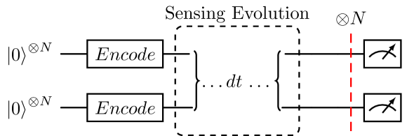
We consider the extension of these results to the dephasing and qubit-flip channel cases, as well as the general setting comprised of and noise. We consider a robust quantum metrology protocol that prepares a probe state as the superposition of codewords of a classical linear code . The state can be reinterpreted as the logical state of a CSS code whose -stabilizers are described by . After encoding the parameter into the state through evolution under the sensing Hamiltonian for time , the protocol measures these -stabilizers to determine . The evolution suffers from dephasing noise, which is relevant for robust quantum metrology [14]. In [15], its consideration was limited to permutation-invariant codes, which are non-linear, where the probe state undergoes a fixed amount of dephasing errors. Furthermore, the only requirement on the Quantum Fisher Information (QFI) was that it remained positive after undergoing the noise channel.
We use a similar setup in Section III, but we instead use a linear code. We use this as a toy example that lays out the intuition for our main result: the Robustness Bound. This is a bound for the scaling behavior of the QFI induced by the probe state, which depends on the weight enumerator of the dual of the code . This bound demonstrates that Heisenberg Scaling is only achievable for non-trivial linear codes when the Hamiltonian is orthogonal to the span of the Lindblad operators, a result that extends the ideas of the HNLS condition to the robust metrology case. Our results challenge the effectiveness of linear codes for magnetic field sensing beyond erasures, specifically for dephasing noise. We complete the picture by considering general Pauli noise that is a mixture of and errors, where we show that Heisenberg Scaling is achievable only under purely errors.
The paper is organized as follows: Section II introduces the necessary background for our paper, Section III motivates the usage of the weight enumerator of the dual code for deriving sensing bounds via a toy example, Section IV details our sensing protocol, Section V introduces our main results, and we finally consider the outlook given our results in Section VI. The appendices in the Supplementary Material provide detailed proofs of the main results.
II Background
II.1 Single Parameter Quantum Metrology
In our work, we wish to sense a classical parameter related to the strength of a weak magnetic field. In this case, our quantum probe state evolves with respect to the Hamiltonian operator:
| (II.1) |
We wish to sense with as little uncertainty as possible, meaning we wish to minimize:
| (II.2) |
where (II.2) is known as the Quantum Cramer-Rao bound [16] and is our Quantum Fisher Information (QFI), defined as follows with respect to some measurement operator is [17]:
| (II.3) |
where and are the set of eigenvalues and eigenvectors of , respectively. The optimal operator to measure for determining (II.3) is the Symmetric Logarithmic Derivative, (SLD), given by [16]:
| (II.4) |
There are two limits of (II.2) that are relevant to our goal: the Heisenberg Limit (HL), which is given by , which is the minimal uncertainty allowed by Quantum Mechanics, and the Standard Quantum Limit, (SQL), which is , where is the number of qubits of the probe state. When the system is noiseless, it can be shown that the -qubit GHZ state gives the optimal probe state for achieving the HL [18]:
| (II.5) |
However, this is no longer true when our system is noisy. Thus, to maximize our QFI, we must first quantify the noisy evolution of the probe state.
II.2 Lindbladian Master Equation
The probe state undergoes noisy evolution, which is non-unitary. In general, the noisy evolution of a density operator is given by some Kraus Operators [19] such that:
| (II.6) |
Here, we enforce the equality in the second inequality. Given a unitary operator , we have
| (II.7) |
This is the solution of the differential equation
| (II.8) |
known as the Liouville-Von Neumann equation. Inserting (II.2) into (II.8), for a Markovian channel, we derive the Lindblad Master-Equation [20]:
Here, we can define our jump operators .
II.3 Code Weight Enumerator
To maximize the QFI of measurements in the presence of noise, we define the probe state to be the equally weighted superposition of codewords of a classical code . The probe state can be reinterpreted as the logical state of a CSS (Calderbank-Shor-Steane) stabilizer code with -stabilizers defined by .
Since we use superpositions of codewords of some code as the probe state, it will be necessary to enumerate the number of codewords of Hamming weight , for all . The weight corresponds to the number of Pauli operators in an -stabilizer derived from a codeword of . The weight enumerator is a polynomial whose coefficients are the number of codewords of each weight in the code :
| (II.9) |
where is some formal variable [21]. As we will show later, the weight enumerator of the dual code of , denoted , will determine the QFI. Given (II.9), we can find the dual code’s weight enumerator by using the MacWilliams identity:
| (II.10) |
To minimize the uncertainty, we must choose a probe state that maximizes QFI, which will depend on (II.10). We will show that it suffices to choose a code whose dual code has many codewords of a certain weight , i.e., that such a code maximizes the QFI for the channel. To demonstrate this, we consider a toy example that gives an intuition for how the QFI is related to (II.10).
III Finding optimal Probe state under a fixed number of errors
We begin with a toy example, where a known amount of flips occur [15]. This example helps demonstrate how the weight enumerator of a code fundamentally determines the QFI of the probe state. Let be an evenly weighted superposition of all the classical codewords in our code , where . Thus, we can write our pure state in density operator form as:
| (III.1) |
Now we write our channel, which applies a gate to exactly qubits, which has an equal probability to flip any set of qubits from our state . This can be written as:
| (III.2) |
where is a special case of the Pauli operator:
| (III.3) |
where , , and is set of all length binary vectors with weight . Applying to yields:
| (III.4) |
where is the dimensional inner product, and is addition over . We can use the following upper bound for the QFI to look at the probe’s behavior, which is tight for a pure state [13]:
| (III.5) |
where the Hamiltonian is given by (II.1), and . Finally, . Inserting (III.4) into (III.5), and looking at the first term of the RHS of our inequality, we can write this as:
| (III.6) | ||||
| (III.7) | ||||
| (III.8) |
where are binary vectors with a single in index and , respectively. Due to the orthonormality of codewords and the trace, the RHS reduces to:
| (III.9) |
Thus, this term is maximized by having many weight 2 dual code words. Similarly, one finds that:
| (III.10) |
where we now wish to minimize the number of weight one dual code words. These tasks can be achieved via expanding (II.10) for the term. We see that to leading order, we can achieve , which would give us Heisenberg Scaling in the pure case. This shows why the GHZ state is optimal for pure unitary channels, since is the repetition code in that case and, therefore, has all even-weight vectors.
IV Robust Quantum Sensing Protocol
Typically, the optimal measurement for finding in quantum metrology is given by Eqn. (II.4). However, since the eigenvectors of Eqn. (II.4) typically depend on , it is challenging to turn this measurement into an explicit measurement that can be implemented in a lab. We find that instead, it is sufficient to measure the syndrome of all the -stabilizers of our code after the probe state has evolved for some time . We can then calculate the probability of measuring all for our syndrome, , by using copies of the probe state, where is the projector constructed from all stabilizers of our code and the subscript corresponds to the syndrome. Repeating this for a sufficient number of longer time steps, we show in Appendix A that our probability will be given by:
| (IV.1) | ||||
Here, is given by:
| (IV.2) |
for the dephasing case, where is the robustness of the code, given by:
| (IV.3) |
Thus, we can recover the parameter with sufficient time steps by taking the Fourier transform of our time-dependent signal. Therefore, we can sense our parameter without relying on rapid and precise control operations at the expense of more significant spatial overhead.
V Main Result
We now generalize our protocol by considering a -qubit dephasing channel, which also depends on the sensing parameter . We find a new bound called the Robustness bound, which demonstrates that the weight enumerator of the dual code encapsulated in (IV.3) determines the scaling behavior of the probe state measurement. Given this bound, we derive the following theorem:
Theorem 1.
Given an -qubit dephasing channel affecting an all- Hamiltonian, no non-trivial linear code can achieve Heisenberg Scaling for robust field sensing.
Here, we find that for the QFI of our measurement to be maximized, we need
| (V.1) |
Specifically, saturating this bound achieves the HL. But due to the form of , only the trivial code with dual code consisting of all weight- vectors saturates the bound, implying that the probe state must be trivial (corresponding to the trivial code ). The proof is given in Appendix A.
We now turn to the case where the noise channel is orthogonal to the Hamiltonian. For this case, we give the following positive result:
Theorem 2.
Given an -qubit bit-flip channel with an all- Hamiltonian, a non-trivial linear code with maximal number of weight- dual codewords can asymptotically achieve Heisenberg Scaling for robust field sensing.
In this case, for any code. The proof is given in Appendix B.
Finally, for the general case, where we have a full-rank channel that mixes the dephasing and bit-flip channels by some polar angle , we show that:
Theorem 3 (Impossibility of Heisenberg-Scaling for Noisy Linear Probes).
Given an -qubit channel with an all- Hamiltonian such that the channel is comprised of tensor products of the operator , a non-trivial linear code can achieve Heisenberg Scaling for robust field sensing if and only if .
Proof of Theorem 3.
It is sufficient to consider the case which lower bounds of the general channel, which is the channel: , where , are the dephasing and bit flip channels from before.
Following the same derivations from Theorems 1 and 2, we see that our dampening function for the approximate case is given as:
| (V.2) |
where is our robustness from before. We see that we recover the dephasing case of for , and the bit-flip case for , respectively. We wish to make (LABEL:general_gamma) as close to zero as possible, which implies that:
| (V.3) |
For the exact general case, we see that , where , and , as shown in Appendix C, thus . This implies that for any , recovering the HL is independent of , since the HL for the robustness bound is only achievable by trivial codes. Thus, the HL is attainable only if . ∎
Since the Robustness of the probe state prevents HL scaling, finite rounds of active error correction will not be able to achieve HL scaling either. Still, they may help achieve an uncertainty closer to saturating the Cramer-Rao bound for the SQL case [22, 1]. However, it should be noted that the HL is attainable if the channel has orthogonal support to the Hamiltonian on a few qubits: i.e., a set of acting on qubits for a Hamiltonian of the form (II.1). Not only is HL attainable for this case, but the choice of the probe state will significantly affect how close we come to saturating the Cramer-Rao bound, but a physical system with such properties remains elusive.
VI Outlook
In this paper, we introduce a robust metrology protocol, which measures by a probe state constructed from some linear code . Our measurement’s uncertainty depends on the Robustness Bound: a quantity derived from the dual-code weight enumerator and the channel. We then show that the Robustness Bound implies that no probe state based on a non-trivial, linear code can achieve the HL without the channel and Hamiltonian being orthogonal. This, in turn, demonstrates that the principles of the HNLS condition remain valid in this regime, even in the absence of active error correction. Although our result limits the efficacy of quantum error correction protocols for metrology applications, we note that in previous work, the HL was shown to be attainable for erasure channels both in the case of finite-round error correction and robust sensing regimes [13, 23], both for linear codes and permutation-invariant codes. This means HL scaling could be attainable by utilizing erasure qubits using a similar setup to what is described here [24]. Another exciting direction for metrology is using non-Markovian dynamics and non-linear Kerr interactions as sensing resources, which have already shown promise in surpassing SQL [9, 25]. Regardless of which approach is considered, there are many open questions about which approach will be the most practical.
Acknowledgements
We thank Christos Gagatsos and Kanu Sinha for their insights into our paper. Their expertise in quantum metrology proved invaluable. The work of O.N. and N.R. was supported by the ARO Grant W911NF-24-1-0080.
Appendix A Proof of Theorem 1
Lemma 4.
Given a general dephasing channel and a probe state constructed from all code words of linear code , to first-order in , the density operator is given by:
| (A.1) | ||||
Proof of Lemma 4.
Let the probe state be given by , where is a non-trivial, linear code. We subject the probe state to the following evolution:
| (A.2) |
where , and is the set of all length binary vectors with weight , and the term comes from the anti-commutator term from the Lindbladian. We also use the following Hamiltonian:
| (A.3) |
where indexes over all weight 1, length binary vectors. To first order, we find our density operator as:
| (A.4) |
We now take the trace with respect to some projector from our POVM: which we define to be the sum of all of our code’s stabilizers:
| (A.5) |
We first evaluate the commutator given in the first term of (A.2). This evaluates to:
| (A.6) |
where we see that for this to be non-zero then . For this to be true, , so only the off-diagonal terms survive. We now evaluate the channel term of (A.2). First, we note that is small, so we approximate it as . Next, we evaluate the dephasing channel as:
| (A.7) | |||||
We expand this sum over k giving:
| (A.8) | |||||
Noticing a lack of a phase on the term, we rewrite (A) as:
| (A.9) |
Here we notice that either , or . We, therefore, write the second term of (A) as:
| (A.10) |
The sum enumerates the number of weight dual codewords in the code, given by the MacWilliams codeword enumerator . But for the sum , we need to be careful as not every term carries the same sign. We now focus on this term: first we swap the order of the sums, and treat each as a one-dimensional code . If , then the sign is , otherwise it is . We can now enumerate the number of weight dual codewords of with , which does not include . Thus we can rewrite (A) as:
| (A.11) | ||||
| (A.12) |
Combining with the first term of (A), we get:
| (A.13) | ||||
Thus, our density operator now has the form:
| (A.14) | ||||
We label the sum over of our second to last term as: , which we define as our Robustness. ∎
Lemma 5.
The probability is given by:
| (A.15) |
Proof of Lemma 5.
We now evaluate the product of with our projector , given by (A.5).
| (A.16) | ||||
where . Taking the trace of (A.16) yields:
| (A.17) | ||||
We can now evaluate the Kronecker Deltas and write (A.17) in terms of a sum over all possible stabilizers, as we evaluate the sum over . This allows us to rewrite the sum in terms of and . We now rewrite the first term to show how it vanishes.
| (A.18) |
Given the Linearity of , any two codewords , . Since each has weight one at i, we look at the index i. There exists some such that , such that for each , such that , has . Exactly codewords have , thus the inner sum evaluates to . By the same logic, the outer sum in must be zero since exactly half of the codewords in have , while the other half has . Thus, the term vanishes. To first order, we then see that our expansion evaluates to:
| (A.19) |
Since our expansion to first order includes no signal term, we use a second order expansion. We now define:
| (A.20) |
and our second order expansion is approximately:
| (A.21) |
Where we recognize this as a dampened cosine function. Thus, our final form for our probability distribution reads:
| (A.22) |
where ideally . However, we must reexamine . The last term in (A.20) can cause , which would mean that our noise channel amplifies our signal instead of dampening it. Such behavior is non-physical, so we must rescale (A.20) as:
| (A.23) |
This shows us that our scaling behavior depends on the derived quantity . ∎
Proof of Theorem 1.
From our probability distribution (A.22), we can write the variance of our measurement as:
| (A.24) |
Where our Classical Fisher Information, CFI, is given by:
| (A.25) |
Inserting (A.22) into (A.25), we see that:
| (A.26) |
For us to recover the Heisenberg Limit, we must let . This implies that:
| (A.27) |
where the bound is saturated by . But this violates the quantum singleton bound, which means saturating this bound is unachievable. We call this quantity the robustness of the code, which is bounded as:
| (A.28) |
Now, we can choose a code that approaches this bound to minimize the variance of the measurement. We see from the form of that maximizing the number of weight dual codewords will achieve the HL. However, since the codewords of must commute with all of its weight one dual code words, each codeword must not have support on each weight one dual codeword for this to be true. Since the HL is reached by having weight one dual codewords, the only allowed state is the all zeros state, which implies that our code must be trivial and cannot accumulate any signal. This is a contradiction. It is also clear that any number of rounds of active error correction will further reduce the signal collected by any probe state in this scenario, as the action of (A.3) on is indistinguishable from a phase error from the channel. This means that this result holds for any number of rounds of active error correction. Therefore, it is not possible for any nontrivial linear code to achieve Heisenberg Scaling for this channel. ∎
Appendix B Proof of Theorem 2
Proof of Theorem 2.
We begin with the following channel:
| (B.1) |
where again the Hamiltonian is given by (A.3), our POVM is given by (A.5), and the probe state is given by the form in Appendix A. Since the derivation for the signal term is identical to the dephasing case, we begin from the noise term:
| (B.2) |
Again, we notice that either , or . Since span all the codewords of , and for any dual codeword and code word , , we can use the dual code weight enumerator again to enumerate the number of .
| (B.3) | ||||
Taking the trace of the product of the first term of the RHS with our POVM, we see that:
| (B.4) | ||||
For the , we consider the set of one dimensional codes . There are two cases: either or not. We count the number of that are dual codewords of both as . Since both , and are one dimensional, we look at the action of . This sends to an equivalent for each . Since the sum over goes over all codewords, we consider a new code , made up of all codewords of each . Then the second term of (LABEL:bitflipenum) can be written as:
| (B.5) | ||||
where . Because each Pauli operator made of all Pauli operators commutes with all other products of Pauli operators, . Taking the trace with respect to (A.5), the trace of can be written as:
| (B.6) | ||||
Therefore, the trace (LABEL:bitflipenum) can be written as:
| (B.7) | |||
Which means that the dampening due to noise here vanishes. The rest of the derivation follows the same logic as before, which leads to:
| (B.8) |
where . Thus by inserting (B.8) into (A.25), we see that:
| (B.9) |
thus, we asymptotically achieve the HL as long as we maximize the number weight 2 dual codewords of our Code. ∎
Appendix C Deriving General Form of
We begin with the following channel:
| (C.1) |
where , the Hamiltonian is given by (A.3), and the probe state is the same form as in Appendix A. We see that for (C.1), that for , the channel reduces to the previous cases. Let us now focus on the noise term of the case where . Here, we can expand the second term of (C.1) as:
| (C.2) | ||||
where is the set of all length binary vectors with weight up to k. Applying the same approach as in Appendix A for the case and Appendix B for the case, taking the trace of the noise term yields a modified version of :
| (C.3) | ||||
where we notice that is equal to the second term when . We wish to show a relationship between the general case and our approximate case in Theorem 3. To do this, we apply a re-scaling to (C.3) by:
| (C.4) |
and since is equal to the second term of (C.3) when , this implies that under our rescaling:
| (C.5) | ||||
Thus, we see that , , which agrees with the conclusions of Theorem 3.
References
- Kapourniotis and Datta [2019] T. Kapourniotis and A. Datta, Phys. Rev. A 100, 022335 (2019), URL https://link.aps.org/doi/10.1103/PhysRevA.100.022335.
- Reiter et al. [2017] F. Reiter, A. S. Sørensen, P. Zoller, and C. Muschik, Nature communications 8, 1822 (2017), URL https://www.nature.com/articles/s41467-017-01895-5.
- Rojkov et al. [2022] I. Rojkov, D. Layden, P. Cappellaro, J. Home, and F. Reiter, Phys. Rev. Lett. 128, 140503 (2022), URL https://link.aps.org/doi/10.1103/PhysRevLett.128.140503.
- Kessler et al. [2014] E. M. Kessler, I. Lovchinsky, A. O. Sushkov, and M. D. Lukin, Phys. Rev. Lett. 112, 150802 (2014), URL https://link.aps.org/doi/10.1103/PhysRevLett.112.150802.
- Dür et al. [2014] W. Dür, M. Skotiniotis, F. Froewis, and B. Kraus, Physical Review Letters 112, 080801 (2014), URL https://journals.aps.org/prl/abstract/10.1103/PhysRevLett.112.080801.
- Layden et al. [2019] D. Layden, S. Zhou, P. Cappellaro, and L. Jiang, Physical review letters 122, 040502 (2019), URL https://journals.aps.org/prl/abstract/10.1103/PhysRevLett.122.040502.
- Unden et al. [2016] T. Unden, P. Balasubramanian, D. Louzon, Y. Vinkler, M. B. Plenio, M. Markham, D. Twitchen, A. Stacey, I. Lovchinsky, A. O. Sushkov, et al., Physical review letters 116, 230502 (2016), URL https://journals.aps.org/prl/abstract/10.1103/PhysRevLett.116.230502.
- Matsuzaki and Benjamin [2017] Y. Matsuzaki and S. Benjamin, Physical Review A 95, 032303 (2017), URL https://journals.aps.org/pra/abstract/10.1103/PhysRevA.95.032303.
- Yang et al. [2024] X. Yang, X. Long, R. Liu, K. Tang, Y. Zhai, X. Nie, T. Xin, J. Li, and D. Lu, Communications Physics 7, 282 (2024), URL https://www.nature.com/articles/s42005-024-01758-8.
- Beau and del Campo [2017] M. Beau and A. del Campo, Phys. Rev. Lett. 119, 010403 (2017), URL https://link.aps.org/doi/10.1103/PhysRevLett.119.010403.
- Zhou et al. [2018] S. Zhou, M. Zhang, J. Preskill, and L. Jiang, Nature communications 9, 78 (2018), URL https://www.nature.com/articles/s41467-017-02510-3.
- Saleem et al. [2024] Z. H. Saleem, M. Perlin, A. Shaji, and S. K. Gray, Phys. Rev. A 109, 052615 (2024), URL https://link.aps.org/doi/10.1103/PhysRevA.109.052615.
- Ouyang and Rengaswamy [2023] Y. Ouyang and N. Rengaswamy, Phys. Rev. A 107, 022620 (2023), URL https://link.aps.org/doi/10.1103/PhysRevA.107.022620.
- Ouyang et al. [2022] Y. Ouyang, N. Shettell, and D. Markham, IEEE Transactions on Information Theory 68, 1809 (2022), URL https://journals.aps.org/pra/abstract/10.1103/PhysRevA.90.062317.
- Ouyang [2014] Y. Ouyang, Phys. Rev. A 90, 062317 (2014), URL https://link.aps.org/doi/10.1103/PhysRevA.90.062317.
- Braunstein and Caves [1994] S. L. Braunstein and C. M. Caves, Phys. Rev. Lett. 72, 3439 (1994), URL https://link.aps.org/doi/10.1103/PhysRevLett.72.3439.
- Helstrom [1969] C. W. Helstrom, Journal of Statistical Physics 1, 231 (1969), URL https://link.springer.com/article/10.1007/BF01007479.
- Eldredge et al. [2018] Z. Eldredge, M. Foss-Feig, J. A. Gross, S. L. Rolston, and A. V. Gorshkov, Phys. Rev. A 97, 042337 (2018), URL https://link.aps.org/doi/10.1103/PhysRevA.97.042337.
- Kraus et al. [1983] K. Kraus, A. Böhm, J. D. Dollard, and W. Wootters, States, Effects, and Operations Fundamental Notions of Quantum Theory: Lectures in Mathematical Physics at the University of Texas at Austin (Springer, 1983).
- Breuer and Petruccione [2002] H.-P. Breuer and F. Petruccione, The theory of open quantum systems (OUP Oxford, 2002).
- Hill [1986] R. Hill, A first course in coding theory (Oxford University Press, 1986).
- Arrad et al. [2014] G. Arrad, Y. Vinkler, D. Aharonov, and A. Retzker, Physical review letters 112, 150801 (2014), URL https://journals.aps.org/prl/abstract/10.1103/PhysRevLett.112.150801.
- Ouyang and Brennen [2024] Y. Ouyang and G. K. Brennen, Finite-round quantum error correction on symmetric quantum sensors (2024), eprint 2212.06285, URL https://arxiv.org/abs/2212.06285.
- Niroula et al. [2024] P. Niroula, J. Dolde, X. Zheng, J. Bringewatt, A. Ehrenberg, K. C. Cox, J. Thompson, M. J. Gullans, S. Kolkowitz, and A. V. Gorshkov, Phys. Rev. Lett. 133, 080801 (2024), URL https://link.aps.org/doi/10.1103/PhysRevLett.133.080801.
- Zhang et al. [2025] J.-D. Zhang, L. Hou, and S. Wang, Quantum Information Processing 24, 1 (2025), URL https://link.springer.com/article/10.1007/s11128-025-04644-6.