Statistical Inference for Heterogeneous Treatment Effect with Right-censored Data from Synthesizing Randomized Clinical Trials and Real-world Data

Abstract

The heterogeneous treatment effect plays a crucial role in precision medicine. There is evidence that real-world data, even subject to biases, can be employed as supplementary evidence for randomized clinical trials to improve the statistical efficiency of the heterogeneous treatment effect estimation. In this paper, for survival data with right censoring, we consider estimating the heterogeneous treatment effect, defined as the difference of the treatment-specific conditional restricted mean survival times given covariates, by synthesizing evidence from randomized clinical trials and the real-world data with possible biases. We define an omnibus confounding function to characterize the effect of biases caused by unmeasured confounders, censoring, outcome heterogeneity, and measurement error, and further, identify it by combining the trial and real-world data. We propose a penalized sieve method to estimate the heterogeneous treatment effect and the confounding function and further study the theoretical properties of the proposed integrative estimators based on the theory of reproducing kernel Hilbert space and empirical process. The proposed methodology is shown to outperform the approach solely based on the trial data through simulation studies and an integrative analysis of the data from a randomized trial and a real-world registry on early-stage non-small-cell lung cancer.

1 Introduction

The average treatment effect is frequently used in a variety of fields such as medicine, social sciences, and econometrics, to assess the effect of a treatment or intervention. However, the average treatment effect implies the similarity of treatment effect across heterogeneous individuals, which is less plausible for some treatments (Yin, Liu, and Geng, 2018). In such a case, it requires considering the heterogeneity of treatment effect. Moreover, in recent years, there has been an increasing interest in precision medicine (Hamburg and Collins, 2010), which is an emerging approach to disease treatment and prevention and emphasizes the consideration of individual patient characteristics for customizing medical treatments. The trends in precision medicine have led to a proliferation of studies for the heterogeneous treatment effect (HTE; Rothwell, 2005; Rothwell et al., 2005) which is a critical path toward precision medicine (Hamburg and Collins, 2010; Collins and Varmus, 2015).

Randomized clinical trials (RCTs) are considered to be highly reliable and the gold standard for treatment effect evaluation since randomization eliminates both measured and unmeasured confounders. Notwithstanding, to adhere strictly to pre-established research protocols, RCTs typically establish stringent criteria for patient eligibility in terms of inclusion and exclusion, thereby restricting sample diversity and limiting external validity. As a consequence, it may fail when generalizing causal effect estimates based on the RCT data to a target population. Furthermore, due to the slow and costly nature of RCTs, the sample size is frequently limited, which may result in inefficiencies when estimating the HTE based solely on the RCT data. On the other hand, with the technological advances in data science, real-world data (RWD) frequently appears in scientific research, such as disease registries, cohorts, biobanks, epidemiological studies, and electronic health records. In contrast to RCTs, the RWD typically are less cost-intensive, include larger sample sizes and longer follow-up periods, and reflect clinical experiences across a broader and more diverse distribution of patients.

Nevertheless, they also present some challenges while providing valuable complementary information about the estimation of treatment effects. The RWD often contain biases that can affect the quality and accuracy of inference and decision making. These biases may arise from various sources such as selection bias, measurement bias, unmeasured confounding, and lack of concurrency. Selection bias occurs when there is a systematic difference in the characteristics of individuals who receive the treatment compared to those who do not. Measurement bias occurs when there are errors or inconsistencies in the measurement or recording of the outcome or covariates. Unmeasured confounding occurs when there are some unmeasured or unaccounted-for covariates that affects both the treatment or exposure being studied and the outcome of interest. Lack of concurrency occurs when there are some differences in factors such as timing or care setting for collecting the data from the RCT and RWD. Beaulieu-Jones et al. (2020) provided a detailed review of the advantages and limitations of using real-world data. Of particular interest is how to address and mitigate these biases, further employ the RWD as supplementary evidence, and combine them with the RCT data to improve the study efficiency and increase the statistical power for estimating the HTE.

The integrative analysis of the RCT data and RWD has received a lot of interests in the literature. Prentice et al. (2008) proposed joint analysis for pooled data; Soares et al. (2014) developed a hierarchical Bayesian model based on network meta-analysis; Efthimiou et al. (2017) proposed and compared various approaches to combing data, including naive data synthesis, design-adjust synthesis, and three-level hierarchical model with the RWD being prior information; Verde and Ohmann (2015) made a comprehensive summary and analysis of meta-analysis methods; Wang and Rosner (2019) extended the concept of propensity score adjustment in a single study to a multi study setting to minimize bias in the RWD, and proposed a propensity score-based Bayesian nonparametric Dirichlet process mixture model; Lee et al. (2023, 2024b) proposed an integrative estimator of average treatment effect. Furthermore, through imputation based on survival outcome regression and weighting based on inverse probability of sampling, censoring, and treatment assignment, Lee, Yang, and Wang (2022) and Lee et al. (2024a) proposed doubly robust estimators for generalizing average treatment effects on survival outcomes from the RCT to a target population. However, these approaches presuppose the absence of biases in the RWD, which is highly improbable in reality. Existing analysis methods for the biases in the RWD mainly conclude instrumental variable methods (e.g., Angrist, Imbens, and Rubin, 1996), negative controls (e.g., Kuroki and Pearl, 2014), and sensitivity analysis (e.g., Robins, Rotnitzky, and Scharfstein, 1999). Yang et al. (2023) introduced a confounding function approach to handle unmeasured confounder bias, leveraging transportability and trial treatment randomization to improve the heterogeneous treatment effect estimator. They leveraged the transportability and trial treatment randomization to identify the HTE and further couple the RCT data and RWD to identify the confounding function, and demonstrated that the rich information of the RWD indeed improves the power of the HTE estimator from both theoretical and practical perspectives. Colnet et al. (2023) provided a comprehensive review of the existing methods for combining the RCT data and RWD for non-survival outcomes of interest.

In clinical trials and biomedical research studies, time to an event or survival time is often the primary outcome of interest, and the right-censored survival data are frequently encountered. For censored survival data, the restricted mean survival time is an easily interpretable, a clinically meaningful summary of the survival function, which is defined as the area under the survival curve up to a pre-specified time. Then a common way to measure the HTE is to define it as the difference in the conditional restricted mean survival time (CRMST) between the treatment and control groups. The existing estimations for the CRMST can be roughly divided into two classes. One uses survival models for hazard rate function. For example, Zucker (1998), Chen and Tsiatis (2001), and Zhang and Schaubel (2011) used the Cox proportional hazards model (Cox, 1972) for the hazard rate function of survival time, and further derived the estimation of the conditional survival function from the relationship between the hazard rate function and the survival function. Another approach is to model the CRMST directly. For example, Tian, Zhao, and Wei (2014) proposed to model the CRMST through a generalized linear regression model, and further estimated the corresponding parameters by constructing an inverse probability censoring weighted estimating function. The estimating equation involved a Kaplan–Meier estimate of the survival function of censored time, and thus the method relied on a strong assumption that censoring time is independent of the covariates of interest. Wang and Schaubel (2018) relaxed such an assumption and proposed to estimate the survival function of censoring time by using the Cox proportional hazards model (Cox, 1972) and further constructed the estimating equation. There are several pieces of literature for the estimation of the CRMST by machine learning such as causal survival forest (Cui et al., 2023) and random forest (Liu and Li, 2021). In addition, there are some other ways to define the HTE for survival data, e.g., Zhao et al. (2015), Cui, Zhu, and Kosorok (2017), and Hu, Ji, and Li (2020).

In this paper, we consider statistical inference for the HTE with right-censored survival data by combing the RCT data and RWD with possible biases. The HTE is defined as the difference in the CRMST between the treatment and control groups. Inspired by Wu and Yang (2022) and Yang et al. (2023), we define an omnibus confounding function to summarize all sources of bias in real-world data. This results in a flexible and generalizable framework that can be applied across a wide range of study designs and data sources. As such, our approach is a valuable tool for researchers and practitioners working in various fields. Its capacity to handle biases in the RWD, without relying on unrealistic assumptions, makes it an essential tool for improving the accuracy and reliability of causal inference in real-world scenarios. In our methodology, the HTE and confounding function are modeled with fully nonparametric models and estimated by minimizing a proposed penalized loss function. For implementing the proposed estimators, a sieve method is utilized to approximate the targeted functional parameters, the HTE, and the confounding function. Furthermore, we derive the convergence rates and local asymptotic normalities of the proposed estimators by using reproducing kernel Hilbert space (RKHS) and empirical process theory. Simulation studies demonstrate the excellent performance of the proposed method, and an illustrative application of the method to the real data reveals some intriguing findings.

The remainder of the paper is structured as follows: Section 2 provides an introduction to some preliminaries, such as notations and definitions of the HTE and confounding function. In Section 3, we introduce the penalized loss function and sieve method for estimating the unknown functional parameters. Section 4 presents the asymptotic properties of the proposed integrative estimators. Section 5 includes simulation studies and an application to a real non-small cell lung cancer dataset for finite sample performance evaluation of the proposed approach. Finally, in Section 6, we present some discussions, and Web Appendix D in supplementary material including the proofs of theoretical results are also provided.

2 Preliminaries

2.1 Notations: HTE and data structure

For two positive sequences $a_{n}$ and $b_{n}$, denote $a_{n}\asymp b_{n}$ if $\lim_{n\rightarrow\infty}a_{n}/b_{n}=c$ for some constant $c>0$. For real numbers $a$ and $b$, let $a\wedge b=\min\{a,b\}$. Let $T$ and $C$ denote the failure time and the censoring time, respectively. Under the right censoring mechanism, the observed variable is $(Y,\Delta)$, where $Y=T\wedge C$ is the observed time and $\Delta=I(T\leq C)$ is the censoring indicator. Let $\boldsymbol{X}=(X_{1},\ldots,X_{p})^{\rm T}$ be the $p$-dimensional covariate and $A\in\{0,1\}$ be the binary treatment, where $A=1$ and $A=0$ indicate the active treatment and the control, respectively. This paper utilizes potential outcomes (Neyman, 1923; Rubin, 1974) as the framework to define causal effects. Specifically, let $T(a)$ denote the potential outcome that corresponds to the given treatment $A=a$ for $a=0,1$. For a restricted time point $L$, the heterogeneous treatment effect (HTE) is defined as

$$\tau(\boldsymbol{X})=E\left\{T(1)\wedge L-T(0)\wedge L\mid\boldsymbol{X}\right\}.$$

We consider two independent data sources, the RCT data, and the RWD. Let $S=1$ denote the RCT participation and $S=0$ denote the RWD participation. Therefore, the structure of the observed data for subject $i$ can be concluded as $(Y_{i},\Delta_{i},\boldsymbol{X}_{i},A_{i},S_{i})$. It is postulated that the data gathered from RCT comprises of ${\cal V}_{1}=\{(Y_{i},\Delta_{i},\boldsymbol{X}_{i},A_{i},S_{i}=1):i=1,\ldots,n_{1}\}$, with sample size $n_{1}$, which represent independent replications of $(Y,\Delta,\boldsymbol{X},A,S=1)$, while the data from RWD is represented by ${\cal V}_{0}=\{(Y_{i},\Delta_{i},\boldsymbol{X}_{i},A_{i},S_{i}=0):i=n_{1}+1,\ldots,n_{1}+n_{0}\}$ with a sample size of $n_{0}$, which are independent copies of $(Y,\Delta,\boldsymbol{X},A,S=0)$. Our research goal is to estimate $\tau(\boldsymbol{X})$ based on the integrative dataset ${\cal V}_{1}\cup{\cal V}_{0}$ containing $n=n_{1}+n_{0}$ samples.

2.2 Identifiability of the HTE

To explore the identifiability of the HTE from the observed data, we impose certain assumptions as follows. [Consistency in the trial] $T=AT(1)+(1-A)T(0)$.

[Positivity of treatment assignment in the trial] $0<c_{1}\leq P(A=1\mid\boldsymbol{X},S=1)\leq c_{2}<1$, where $c_{1}$ and $c_{2}$ are some constants.

[Mean conditional exchangeability in the trial] $E\{T(a)\wedge L\mid\boldsymbol{X},A,S=1\}=E\{T(a)\wedge L\mid\boldsymbol{X},S=1\}$ for $a=0,1$.

[Transportability in the trial] $E\{T(1)\wedge L-T(0)\wedge L\mid\boldsymbol{X},S=1\}=\tau(\boldsymbol{X})$.

[Conditionally independent censoring in the trial] $T(a)\perp C\mid(\boldsymbol{X},A,S=1)$ for $a=0,1$.

$P(Y\geq L\mid\boldsymbol{X},A,S=1)>0$.

Assumption 2.2 requires no interference between subjects and treatment version irrelevance in the RCT (e.g., Dahabreh et al., 2021). Assumption 2.2 implies that each subject in the RCT has a positive probability of receiving treatment. It is also considered as a fundamental assumption. Assumption 2.2 is satisfied by default for the RCT. Of note, this assumption is formally weaker than the strong ignorability assumption on trial participation, i.e., $T(a)\perp A\mid(\boldsymbol{X},S=1)$ for $a=0,1$, which is a traditional assumption in causal inference. Assumption 2.2 serves as the fundamental basis of this paper and necessitates that the HTE is transportable from the RCT to the target population. This assumption is weaker than the ignorability assumption on trial participation (e.g., Stuart et al., 2011; Buchanan et al., 2018) and the mean exchangeability assumption (e.g., Dahabreh, Robertson, and Hernán, 2019). Assumptions 2.2 and 2.2 are the standard assumptions in survival analysis. Assumption 2.2 is weaker than the conditional independence assumption of the censoring and survival time given only on the treatment (Zhang and Schaubel, 2012). Assumption 2.2 is a classical assumption in survival analysis and guarantees that the observed survival time can possess values within the vicinity of the restricted time point $L$. Particularly, these Assumptions are exclusively imposed on the RCT and not on the RWD, thereby extensively broadening the scope of the proposed methodology.

Let $T_{L}=A\{T(1)\wedge L\}+(1-A)\{T(0)\wedge L\}$, $Y_{L}=Y\wedge L$, $e(\boldsymbol{X})=P(A=1\mid\boldsymbol{X},S=1)$ be the treatment propensity score, and $\mu_{a}(\boldsymbol{X})=E(T_{L}\mid\boldsymbol{X},A=a,S=1)$ with $a=0,1$. We now deliberate on the identifiability of the HTE from the RCT data. If the failure time $T$ is precisely observed for all subjects, to identify the HTE, we can use the method proposed by Lee, Okui, and Whang (2017), in which an augmented inverse probability weighting (AIPW) approach is proposed for complete data. To be specific, let

$$R_{1}=\frac{AT_{L}}{e(\boldsymbol{X})}-\frac{A-e(\boldsymbol{X})}{e(\boldsymbol{X})}\mu_{1}(\boldsymbol{X}),\quad R_{0}=\frac{(1-A)T_{L}}{1-e(\boldsymbol{X})}+\frac{A-e(\boldsymbol{X})}{1-e(\boldsymbol{X})}\mu_{0}(\boldsymbol{X}),\quad R=R_{1}-R_{0}.$$

Under Assumptions 1–4, Proposition S1 in Web Appendix B shows that

$$E(R\mid\boldsymbol{X},S=1)=\tau(\boldsymbol{X}),$$ (1)

which indicators the identifiability of $\tau(\cdot)$ from the RCT data in the uncensored case.

To handle the right censoring, an augmented inverse probability-of-censoring weighting (AIPCW) method (Zhao et al., 2015) is employed in this paper. Let $G_{T}(t\mid\boldsymbol{X},A,S=1)=P(T\geq t\mid\boldsymbol{X},A,S=1)$ and $G_{C}(t\mid\boldsymbol{X},A,S=1)=P(C\geq t\mid\boldsymbol{X},A,S=1)$ be the conditional survival functions of the failure time $T$ and censoring time $C$ given $\boldsymbol{X}$, $A$ and $S=1$, respectively. Let $\widetilde{\Delta}=I(T_{L}\leq C)$, $N_{C}(t)=(1-\widetilde{\Delta})I(Y_{L}\leq t)$, $Q_{C}(t)=\int_{0}^{t}I(Y_{L}\geq u)G^{-1}_{C}(u\mid\boldsymbol{X},A,S=1){\rm d}G_{C}(u\mid\boldsymbol{X},A,S=1)$, $M_{C}(t)=N_{C}(t)+Q_{C}(t)$, $B(t)=E(T_{L}\mid T_{L}>t,\boldsymbol{X},A,S=1)=t+{\int_{t}^{L}G_{T}(u\mid\boldsymbol{X},A,S=1){\rm d}u}/{G_{T}(t\mid\boldsymbol{X},A,S=1)}$, and further

$$\widetilde{T}_{L}={Y_{L}\widetilde{\Delta}}{G^{-1}_{C}(Y_{L}\mid\boldsymbol{X},A,S=1)}-\int_{0}^{L}B(t)G^{-1}_{C}(t\mid\boldsymbol{X},A,S=1){\rm d}M_{C}(t).$$

Then, under Assumptions 5 and 6, Proposition S2 in Web Appendix B shows that

$$E\left(\widetilde{T}_{L}\mid\boldsymbol{X},A,S=1\right)=E\left({T}_{L}\mid\boldsymbol{X},A,S=1\right).$$ (2)

Consequently, defining $\widetilde{R}$ by replacing $T_{L}$ with $\widetilde{T}_{L}$ in the definition of $R$ and further combining equations (1) and (2), we obtain

$$E\left(\widetilde{R}\mid\boldsymbol{X},S=1\right)=\tau(\boldsymbol{X}),$$ (3)

under Assumptions 1–6. That is, the HTE $\tau(\cdot)$ can be identified from the RCT data.

For the RWD, we define the confounding function

$$\lambda(\boldsymbol{X})=E\left(Y_{L}\mid\boldsymbol{X},S=0\right)-\tau(\boldsymbol{X}).$$ (4)

Let $D=S\,\widetilde{R}+(1-S)\,Y_{L}$ and combine equations (3) and (4),

$$E\left(D\mid\boldsymbol{X},S\right)=\tau(\boldsymbol{X})+(1-S)\lambda(\boldsymbol{X}),$$ (5)

which implies the identifiability of $\tau(\cdot)$ and $\lambda(\cdot)$ from the integrative dataset ${\cal V}_{1}\cup{\cal V}_{0}$.

3 Estimation methodology

Let $\sigma^{2}(\boldsymbol{x},s)=\sigma^{2}_{s}(\boldsymbol{x})={\rm Var}(D\mid\boldsymbol{X}=\boldsymbol{x},S=s)$. Based on the integrative dataset ${\cal V}_{1}\cup{\cal V}_{0}=\{(Y_{i},\Delta_{i},\boldsymbol{X}_{i},A_{i},S_{i}),i=1,\ldots,n\}$, equation (5) enables us to construct the loss function with respect to $\tau(\cdot)$ and $\lambda(\cdot)$ as

$${\ell}_{n}(\tau,\lambda)=\frac{1}{2n}\sum_{i=1}^{n}\left\{\sigma^{2}(\boldsymbol{X}_{i},S_{i})\right\}^{-1}\left\{{D}_{i}-\tau(\boldsymbol{X}_{i})-(1-S_{i})\lambda(\boldsymbol{X}_{i})\right\}^{2}.$$

Then an estimated version of loss function ${\ell}_{n}(\tau,\lambda)$ can be written as

$$\widehat{\ell}_{n}(\tau,\lambda)=\frac{1}{2n}\sum_{i=1}^{n}\left\{\widehat{\sigma}^{2}(\boldsymbol{X}_{i},S_{i})\right\}^{-1}\big{\{}\widehat{D}_{i}-\tau(\boldsymbol{X}_{i})-(1-S_{i})\lambda(\boldsymbol{X}_{i})\big{\}}^{2},$$

where $\widehat{D}=S\,\widehat{R}+(1-S)\,Y_{L}$, $\widehat{R}$ is defined by replacing ${e}(\boldsymbol{X})$, ${\mu}_{a}(\boldsymbol{X})$, ${G}_{T}(t\mid\boldsymbol{X},A,S=1)$, and ${G}_{C}(t\mid\boldsymbol{X},A,S=1)$ with the estimators $\widehat{e}(\boldsymbol{X})$, $\widehat{\mu}_{a}(\boldsymbol{X})$, $\widehat{G}_{T}(t\mid\boldsymbol{X},A,S=1)$, and $\widehat{G}_{C}(t\mid\boldsymbol{X},A,S=1)$ in the definition of $\widetilde{R}$, respectively, and $\widehat{\sigma}^{2}(\boldsymbol{X},S)$ is the estimator of ${\rm Var}({D}\mid\boldsymbol{X},S)$.

For a multi-index vector $k=(k_{1},\ldots,k_{p})$ of non-negative integers and a differentiable function $f(\boldsymbol{x})$ with $\boldsymbol{x}=(x_{1},\ldots,x_{p})^{\rm T}$, we define $|k|=k_{1}+\ldots+k_{p}$ and the corresponding $k$-th order derivative of $f(\boldsymbol{x})$ as $f^{(k)}(\boldsymbol{x})={\partial^{k}f(\boldsymbol{x})}/(\partial x_{1}^{k_{1}}\ldots\partial x_{p}^{k_{p}})$. Suppose that the covariate $\boldsymbol{X}$ is taken values in an open connect set $\Omega$ with $C^{\infty}$ boundary. For $m^{\prime}_{1}>p/2$, we define the $m^{\prime}_{1}$-th order Sobolev space ${\cal H}_{1}$ as

$${\cal H}_{1} = \bigg{\{}f:\Omega\rightarrow\mathbb{R}\,\big{|}\,f^{(j)}\textrm{ is absolutely continuous for }|j|=0,1,\ldots,(m^{\prime}_{1}-1),$$

$$\textrm{ and }f^{(k)}\in L_{2}(\Omega)\textrm{ for }|k|=m^{\prime}_{1}\bigg{\}},$$

where $L_{2}(\Omega)$ is the collection of all square-integrable functions defined on $\Omega$. Similarly, we define the $m^{\prime}_{0}$-th order Sobolev space ${\cal H}_{0}$ for $m^{\prime}_{0}>p/2$. Let $\tau_{0}(\cdot)$ and $\lambda_{0}(\cdot)$ be the true values of $\tau(\cdot)$ and $\lambda(\cdot)$. Throughout the paper, we suppose $\tau_{0}(\cdot)$ and $\lambda_{0}(\cdot)$ belong to ${\cal H}_{1}$ and ${\cal H}_{0}$, respectively. For $p/2<m_{1}\leq m_{1}^{\prime}$, $p/2<m_{0}\leq m_{0}^{\prime}$, $k=(k_{1},\ldots,k_{p})$, $k^{\prime}=(k^{\prime}_{1},\ldots,k^{\prime}_{p})$, $f,\widetilde{f}\in{\cal H}_{1}$, and $g,\widetilde{g}\in{\cal H}_{0}$, define

$$J_{1}(f,\widetilde{f}) = \sum_{|k|=m_{1}}\frac{m_{1}!}{\prod_{j=1}^{p}k_{j}!}\int_{\Omega}f^{(k)}(\boldsymbol{x})\widetilde{f}^{(k)}(\boldsymbol{x}){\rm d}\boldsymbol{x},$$

$$J_{0}(g,\widetilde{g}) = \sum_{|k^{\prime}|=m_{0}}\frac{m_{0}!}{\prod_{j=1}^{p}k^{\prime}_{j}!}\int_{\Omega}g^{(k^{\prime})}(\boldsymbol{x})\widetilde{g}^{(k^{\prime})}(\boldsymbol{x}){\rm d}\boldsymbol{x}.$$

Then, we propose the penalized loss function for $\tau(\cdot)$ and $\lambda(\cdot)$ as

$$\widehat{\ell}_{n,\gamma_{1},\gamma_{0}}(\tau,\lambda)=\widehat{\ell}_{n}(\tau,\lambda)+\frac{\gamma_{1}}{2}J_{1}(\tau,\tau)+\frac{\gamma_{0}}{2}J_{0}(\lambda,\lambda),$$

where $\gamma_{1}$ and $\gamma_{0}$ are some positive penalized parameters and converge to zero as the sample size $n$ goes to infinity.

For inferring $\tau_{0}(\cdot)$ and $\lambda_{0}(\cdot)$, we use sieve expansion to approximate $\tau(\cdot)$ and $\lambda(\cdot)$ in $\widehat{\ell}_{n,\gamma_{1},\gamma_{0}}(\tau,\lambda)$. Specifically, let $\{\phi_{1}(\cdot),\ldots,\phi_{r_{1}}(\cdot)\}$ and $\{\psi_{1}(\cdot),\ldots,\psi_{r_{0}}(\cdot)\}$ denote two sets of sieve basis functions, and let $\Phi_{n}$ and $\Psi_{n}$ be the corresponding spanned linear spaces, respectively, where $r_{1}$ and $r_{0}$ are the numbers of basis functions and represent the complexities of the approximations. Then, we propose the estimator of $(\tau_{0},\lambda_{0})$ as

$$(\widehat{\tau}_{n},\widehat{\lambda}_{n})=\arg{\min}_{(\tau,\lambda)\in\Phi_{n}\times\Psi_{n}}\widehat{\ell}_{n,\gamma_{1},\gamma_{0}}(\tau,\lambda).$$

4 Asymptotic Properties

Suppose that $n_{1}/n\rightarrow\varrho$ as $n\rightarrow\infty$, where $0<\varrho<1$. Let $\sigma_{0s}^{2}(\boldsymbol{x})$ denote the probability limit of $\widehat{\sigma}^{2}_{s}(\boldsymbol{x})$, and $q_{1}(\boldsymbol{x})$ and $q_{0}(\boldsymbol{x})$ denote the density functions of $\boldsymbol{X}$ for the RCT and RWD, respectively. For $f,\widetilde{f}\in{\cal H}_{1}$ and $g,\widetilde{g}\in{\cal H}_{0}$, define

$$V_{1}(f,\widetilde{f}) = \int_{\Omega}\left[\varrho\left\{\sigma^{2}_{01}(\boldsymbol{x})\right\}^{-1}q_{1}(\boldsymbol{x})+(1-\varrho)\left\{\sigma^{2}_{00}(\boldsymbol{x})\right\}^{-1}q_{0}(\boldsymbol{x})\right]f(\boldsymbol{x})\widetilde{f}(\boldsymbol{x}){\rm d}\boldsymbol{x},$$

$$V_{0}(g,\widetilde{g}) = (1-\varrho)\int_{\Omega}\left\{\sigma^{2}_{00}(\boldsymbol{x})\right\}^{-1}g(\boldsymbol{x})\widetilde{g}(\boldsymbol{x})q_{0}(\boldsymbol{x}){\rm d}\boldsymbol{x}.$$

Then ${\cal H}_{1}$ is a reproducing kernel Hilbert space (RKHS) endowed with the inner product $\langle f,\widetilde{f}\rangle_{{\cal H}_{1}}=V_{1}(f,\widetilde{f})+\gamma_{1}J_{1}(f,\widetilde{f})$ and the norm $\|f\|^{2}_{{\cal H}_{1}}=\langle f,f\rangle_{{\cal H}_{1}}$, and ${\cal H}_{0}$ is a RKHS endowed with the inner product $\langle g,\widetilde{g}\rangle_{{\cal H}_{0}}=V_{0}(g,\widetilde{g})+\gamma_{0}J_{0}(g,\widetilde{g})$ and the norm $\|g\|^{2}_{{\cal H}_{0}}=\langle g,g\rangle_{{\cal H}_{0}}$. Define the product space ${\cal H}={\cal H}_{1}\times{\cal H}_{0}$ endowed with the inner product $\langle\boldsymbol{h},\widetilde{\boldsymbol{h}}\rangle_{{\cal H}}=\langle f,\widetilde{f}\rangle_{{\cal H}_{1}}+\langle g,\widetilde{g}\rangle_{{\cal H}_{0}}$ and the norm $\|\boldsymbol{h}\|_{{\cal H}}^{2}=\langle\boldsymbol{h},{\boldsymbol{h}}\rangle_{{\cal H}}=\|f\|_{{\cal H}_{1}}^{2}+\|g\|_{{\cal H}_{0}}^{2}$ for $\boldsymbol{h}=(f,g)\in{\cal H}$ and $\widetilde{\boldsymbol{h}}=(\widetilde{f},\widetilde{g})\in{\cal H}$.

Let $K_{1}(\cdot,\cdot)$ and $K_{0}(\cdot,\cdot)$ denote the reproducing kernels for ${\cal H}_{1}$ and ${\cal H}_{0}$, respectively, then $K_{1}(\cdot,\cdot)$ and $K_{0}(\cdot,\cdot)$ are known to have the properties $K_{1\boldsymbol{x}}(\cdot)\equiv K_{1}(\boldsymbol{x},\cdot)=K_{1}(\cdot,\boldsymbol{x})\in{\cal H}_{1}$ and $\langle K_{1\boldsymbol{x}},f\rangle_{{\cal H}_{1}}=f(\boldsymbol{x})$, and $K_{0\boldsymbol{x}}(\cdot)\equiv K_{0}(\boldsymbol{x},\cdot)=K_{0}(\cdot,\boldsymbol{x})\in{\cal H}_{0}$ and $\langle K_{0\boldsymbol{x}},g\rangle_{{\cal H}_{0}}=g(\boldsymbol{x})$. We further define two nonnegative definite and self-adjoint linear operators $W_{\gamma_{1}}$ and $W_{\gamma_{0}}$ respectively defined on ${\cal H}_{1}$ and ${\cal H}_{0}$ such that $\langle W_{\gamma_{1}}f,\widetilde{f}\rangle_{{\cal H}_{1}}=\gamma_{1}J_{1}(f,\widetilde{f})$ for $f,\widetilde{f}\in{\cal H}_{1}$, and $\langle W_{\gamma_{0}}g,\widetilde{g}\rangle_{{\cal H}_{0}}=\gamma_{0}J_{0}(g,\widetilde{g})$ for $g,\widetilde{g}\in{\cal H}_{0}$. Then $\langle f,\widetilde{f}\rangle_{{\cal H}_{1}}=V_{1}(f,\widetilde{f})+\langle W_{\gamma_{1}}f,\widetilde{f}\rangle_{{\cal H}_{1}}$ and $\langle g,\widetilde{g}\rangle_{{\cal H}_{0}}=V_{0}(g,\widetilde{g})+\langle W_{\gamma_{0}}g,\widetilde{g}\rangle_{{\cal H}_{0}}$.

Theorem 4.1

Assuming that Assumptions 2.2–2.2 are met, as well as Conditions S1–S6 as outlined in Web Appendix A. Then

$$\|\widehat{\tau}_{n}-{\tau}_{0}\|_{{\cal H}_{1}}=o_{P}(1),\quad\left\|\widehat{\lambda}_{n}-\lambda_{0}\right\|_{{\cal H}_{0}}=o_{P}(1).$$

Given that $\mu_{a}(\boldsymbol{X})=E(T_{L}\mid\boldsymbol{X},A=a,S=1)=\int_{0}^{L}G_{T}(t\mid\boldsymbol{X},A=a,S=1){\rm d}t$, using $\widehat{\mu}_{a}(\boldsymbol{X})=\int_{0}^{L}\widehat{G}_{T}(t\mid\boldsymbol{X},A=a,S=1){\rm d}t$ as an estimator for $\mu_{a}(\boldsymbol{X})$ is appropriate. In this context, Theorem 4.1 implies that if $\widehat{G}_{T}(t\mid\boldsymbol{X},A,S=1)$ is consistent, or both $\widehat{G}_{C}(t\mid\boldsymbol{X},A,S=1)$ and $\widehat{e}(\boldsymbol{X})$ are consistent, then $\widehat{\tau}_{n}(\cdot)$ and $\widehat{\lambda}_{n}(\cdot)$ are consistent estimators of $\tau_{0}(\cdot)$ and $\lambda_{0}(\cdot)$, respectively. For the RCT, where the probability of receiving treatment is typically known, Theorem 4.1 establishes that if either $\widehat{G}_{T}$ or $\widehat{G}_{C}$ is consistent, $\widehat{\tau}_{n}$ and $\widehat{\lambda}_{n}$ remain consistent. In such a case, Theorem 4.1 thus highlights the double robustness of the proposed HTE estimator, an important attribute that enhances its reliability. Alternatively, regardless of the knowledge of $e(\boldsymbol{X})$, one can use a nonparametric estimation approach for $\mu_{a}(\boldsymbol{X})$. Employing such methods ensures consistency, thereby providing reliable estimators for $\widehat{\tau}_{n}$ and $\widehat{\lambda}_{n}$. Under stronger assumptions, Theorem 4.2 provides the convergence rates of the proposed estimators, making it a strengthened version of Theorem 4.1.

Theorem 4.2

Assuming that Assumptions 2.2–2.2 are met, as well as Conditions S1–S5, and S7–S9 as outlined in Web Appendix A. Then

$$\|\widehat{\tau}_{n}-\tau_{0}\|_{{\cal H}_{1}} = O_{P}(n^{-1/2}\gamma_{1}^{-p/(4m_{1})}+n^{-1/2}\gamma_{0}^{-p/(4m_{0})}+\gamma_{1}^{1/2}+\gamma_{0}^{1/2}),$$

$$\|\widehat{\lambda}_{n}-\lambda_{0}\|_{{\cal H}_{0}} = O_{P}(n^{-1/2}\gamma_{1}^{-p/(4m_{1})}+n^{-1/2}\gamma_{0}^{-p/(4m_{0})}+\gamma_{1}^{1/2}+\gamma_{0}^{1/2}).$$

Remark 4.3

If $m_{1}=m_{0}=m$ and $\gamma_{1}\asymp\gamma_{0}\asymp n^{-2m/(2m+p)}$, then $\widehat{\tau}_{n}$ and $\widehat{\lambda}_{n}$ achieve the same optimal convergence rate of $O_{P}(n^{-m/(2m+p)})$, which is also the optimal rate in the most commonly used nonparametric methods.

Let $\dot{\widehat{\boldsymbol{U}}}_{n}(\tau,\lambda)$ denote the second order Fréchet derivative operator of $\widehat{\ell}_{n}(\tau,\lambda)$ with respective to $(\tau,\lambda)$, $\dot{\boldsymbol{U}}(\tau,\lambda)$ denote the probability limit of $\dot{\widehat{\boldsymbol{U}}}_{n}(\tau,\lambda)$, and $\dot{\boldsymbol{W}}_{\boldsymbol{\gamma}}$ denote the linear operator map ${\cal H}$ to ${\cal H}$ such that $\dot{\boldsymbol{W}}_{\boldsymbol{\gamma}}[\boldsymbol{h}]=(W_{\gamma_{1}}f,W_{\gamma_{0}}g)$ for $\boldsymbol{h}=(f,g)\in{\cal H}$. Let $\dot{\boldsymbol{U}}_{\boldsymbol{\gamma}}(\tau,\lambda)=\dot{\boldsymbol{U}}(\tau,\lambda)+\dot{\boldsymbol{W}}_{\boldsymbol{\gamma}}$ and $\dot{\boldsymbol{U}}_{\boldsymbol{\gamma}}^{-1}(\tau,\lambda)$ denote the inverse operator of $\dot{\boldsymbol{U}}_{\boldsymbol{\gamma}}(\tau,\lambda)$.

Theorem 4.4

Assuming that assumptions in Theorem 4.2 are met, as well as Conditions S10–S14 as outlined in Web Appendix A. Then given $x_{0}\in\Omega$, we have

$$\left(n^{1/2}\gamma_{1}^{p/(4m_{1})}\{\widehat{\tau}_{n}(\boldsymbol{x}_{0})-\tau^{*}_{0}(\boldsymbol{x}_{0})\},n^{1/2}\gamma_{0}^{p/(4m_{0})}\{\widehat{\lambda}_{n}(\boldsymbol{x}_{0})-\lambda^{*}_{0}(\boldsymbol{x}_{0})\}\right)^{\rm T}\rightsquigarrow N(0,\boldsymbol{\Sigma}),$$

where $\rightsquigarrow$ denotes convergence in distribution, $\tau_{0}^{*}=\tau_{0}-b_{\tau},\lambda_{0}^{*}=\lambda_{0}-b_{\lambda}$ with $(b_{\tau},b_{\lambda})=\dot{\boldsymbol{U}}^{-1}_{\boldsymbol{\gamma}}(\tau_{0},\lambda_{0})[(W_{\gamma_{1}}\tau_{0},W_{\gamma_{0}}\lambda_{0})]$, and $\boldsymbol{\Sigma}$ is the covariance matrix such that, for every $\boldsymbol{\omega}=(\omega_{1},\omega_{0})^{\rm T}\in\mathbb{R}^{2}$,

$$\boldsymbol{\omega}^{\rm T}\boldsymbol{\Sigma}\boldsymbol{\omega}=\lim_{n\rightarrow\infty}\left\{V_{1}(K_{1}^{*},K_{1}^{*})+V_{0}(K_{0}^{*},K_{0}^{*})+2(1-\varrho)\int_{\Omega}\left\{\sigma^{2}_{00}(\boldsymbol{x})\right\}^{-1}K_{1}^{*}(\boldsymbol{x})K_{0}^{*}(\boldsymbol{x})q_{0}(\boldsymbol{x}){\rm d}\boldsymbol{x}\right\}$$

with $(K_{1}^{*},K_{0}^{*})=\dot{\boldsymbol{U}}^{-1}_{\boldsymbol{\gamma}}(\tau_{0},\lambda_{0})[(\omega_{1}\gamma_{1}^{p/(4m_{1})}K_{1\boldsymbol{x}_{0}},\omega_{0}\gamma_{0}^{p/(4m_{0})}K_{0\boldsymbol{x}_{0}})]$.

Theorem 4.4 demonstrates the pointwise asymptotic normality of $(\widehat{\tau}_{n},\widehat{\lambda}_{n})$ and indicates that the proposed integrative estimator is biased by the penalized component $(W_{\gamma_{1}}\tau_{0},W_{\gamma_{0}}\lambda_{0})$. Analyzing the bias is challenging, however, it can be disregarded under specific undersmoothing conditions, as shown in Corollary 4.5.

Corollary 4.5

Suppose that assumptions in Theorem 4.4 hold, furthermore, $n(\gamma_{1}+\gamma_{0})=O(1)$. Then given $\boldsymbol{x}_{0}\in\Omega$,

$$\left(n^{1/2}\gamma_{1}^{p/(4m_{1})}\{\widehat{\tau}_{n}(\boldsymbol{x}_{0})-\tau_{0}(\boldsymbol{x}_{0})\},n^{1/2}\gamma_{0}^{p/(4m_{0})}\{\widehat{\lambda}_{n}(\boldsymbol{x}_{0})-\lambda_{0}(\boldsymbol{x}_{0})\}\right)^{\rm T}\rightsquigarrow N(0,\boldsymbol{\Sigma}).$$

Let $\widehat{\tau}_{\rm rct}(\cdot)$ denote the estimator of $\tau_{0}(\cdot)$ derived solely from the trial data. The last aim is to theoretically show that the proposed integrative method is more efficient than using only the trial data, specifically ${\rm Var}\{\widehat{\tau}_{n}(\boldsymbol{x}_{0})\}\leq{\rm Var}\{\widehat{\tau}_{\rm rct}(\boldsymbol{x}_{0})\}$. However, the estimators involve estimating nuisance functions, which makes calculating the variances very complex. For simplification, under some stronger conditions and treating nuisance functions as known, we show the proposed method has the advantage of gaining efficiency in estimating $\tau(\cdot)$, which summarized in Theorem 4.6.

Theorem 4.6

Assuming that Assumptions 2.2–2.2 are met, as well as Conditions S1–S3, and S15–S17 as outlined in Web Appendix A. Then given $\boldsymbol{x}_{0}\in\Omega$,

$${\rm Var}\{\widehat{\tau}_{n}(\boldsymbol{x}_{0})\}\leq{\rm Var}\{\widehat{\tau}_{\rm rct}(\boldsymbol{x}_{0})\}.$$

5 Numerical Studies

5.1 Simulation study

In this section, we conduct some simulation studies to provide technical support for the application of the proposed method. We consider various types of bias that exist in the real-world study, including selection bias, censoring, outcome heterogeneity, and unmeasured confounding. We focus on the case $p=2$, that is $\boldsymbol{X}=(X_{1},X_{2})^{\rm T}$. Tensor B-splines are employed to get the sieve basis. Specifically, for $\boldsymbol{x}=(x_{1},x_{2})^{\rm T}\in\Omega$, let $\boldsymbol{B}_{1}(x_{1})=(B_{11}(x_{1}),\ldots,B_{1l_{1}}(x_{1}))^{\rm T}$ and $\boldsymbol{B}_{2}(x_{2})=(B_{12}(x_{2}),\ldots,B_{1l_{2}}(x_{2}))^{\rm T}$ be two sets of spline basis functions, then the sieve basis function $\boldsymbol{\phi}(\boldsymbol{x})=\boldsymbol{\phi}(x_{1},x_{2})=(\phi_{1}(x_{1},x_{2}),\ldots,\phi_{r_{1}}(x_{1},x_{2}))^{\rm T}$ is defined as $\boldsymbol{\phi}(x_{1},x_{2})=\boldsymbol{B}_{1}(x_{1})\otimes\boldsymbol{B}_{2}(x_{2})$ with $r_{1}=l_{1}\times l_{2}$, where $\otimes$ is the Kronecker product. Furthermore, the sieve basis function $\boldsymbol{\psi}(\cdot)=(\psi_{1}(\cdot),\ldots,\psi_{r_{0}}(\cdot))^{\rm T}$ for approximating $\lambda(\cdot)$ can be obtained in a similar way. In the simulation, $\widehat{G}_{T}$ and $\widehat{G}_{C}$ is obtained by fitting a Cox proportional hazards model (Cox, 1972), furthermore, $\widehat{\mu}_{a}(\boldsymbol{X})=\int_{0}^{L}\widehat{G}_{T}(t\mid\boldsymbol{X},A=a,S=1){\rm d}t$, where $a=0,1$. $\widehat{\sigma}^{2}_{s}(\boldsymbol{x})$ is obtained by a kernel estimation method and the corresponding bandwidth is selected by the generalized cross-validation (GCV), where $s=0,1$. The penalized parameters $\gamma_{1}$ and $\gamma_{0}$ are also selected by GCV. For comparison, we consider the estimates based only on the RCT data as well.

Throughout the simulation, $e(\boldsymbol{X})=P(A=1\mid\boldsymbol{X},S=1)=0.5$ is known, and the censoring rate is set around $40\%$ for the RCT data and $70\%$ for the RWD. We consider three cases, each representing different scenarios. Case 1 corresponds to the situation where the failure time model is correctly specified, and $E(T_{L}\mid\boldsymbol{X},A,S=1)=E(T_{L}\mid\boldsymbol{X},A,S=0)$. Case 2 corresponds to the situation where the failure time model is correctly specified, but $E(T_{L}\mid\boldsymbol{X},A,S=1)\neq E(T_{L}\mid\boldsymbol{X},A,S=0)$. Case 3 addresses the situation where the failure time model is incorrectly specified, and $E(T_{L}\mid\boldsymbol{X},A,S=1)=E(T_{L}\mid\boldsymbol{X},A,S=0)$. The specific settings are as follows.

Case 1.

For both the RCT data and the RWD, we generate the unmeasured confounder $X_{u}$ from an exponential distribution with a parameter of $5$. For the RCT data, the covariates $X_{1}$ and $X_{2}$ are generated in the following way. We first generate $\widetilde{X}_{1}$ and $\widetilde{X}_{2}$ from standard normal distributions, and further let $X_{1}=4\{\widetilde{X}_{1}-\min(\widetilde{X}_{1})\}/\{\max(\widetilde{X}_{1})-\min(\widetilde{X}_{1})\}-2$, and $X_{2}=4\{\widetilde{X}_{2}-\min(\widetilde{X}_{2})\}/\{\max(\widetilde{X}_{2})-\min(\widetilde{X}_{2})\}-2$. In contrast, for the RWD, $X_{1}$ and $X_{2}$ are generated from a uniform distribution on $(-1,1)$, furthermore, conditional on $X_{1},X_{2}$, and $X_{u}$, the treatment $A$ is generated from a Bernoulli distribution with success probability $P(A=1\mid X_{1},X_{2},X_{u})={\rm expit}\{0.1(X_{1}+X_{2}-X_{u}+1)\}$, where ${\rm expit}(x)=\exp(x)/\{1+\exp(x)\}$. For both the RCT data and RWD, the failure time $T$ is generate from the survival function $G_{T}(t\mid X_{1},X_{2},A,X_{u})=(1+0.02t)\exp\{-0.1X_{u}t-0.2t\exp(-0.2X_{1}-0.5X_{2}+0.4AX_{1}+1.3AX_{2})\}$, and the censoring time $C$ is generated from a Cox model with the conditional hazard function taking the form $h_{C}(t\mid X_{1},X_{2})=h_{0C}(t)\exp(0.5X_{1}+0.5X_{2})$, where $h_{0C}(t)$ is the baseline hazard function. We set $h_{0C}(t)=1.84\times 10^{-2}$ with a study duration of $4.9$ for the RCT data, and $h_{0C}(t)=0.452$ with a study duration of $4.5$ for the RWD to achieve the preset censoring rates. We consider the restricted time point $L=3$, the sample size $(n_{1},n_{0})=(500,1000)$ and $(1000,2000)$. For each configuration, 1000 simulations are repeated.

Case 2.

For the RCT data, $X_{1}$ and $X_{2}$ follow the standard normal distribution, and the failure time $T$ is generate from a Cox model $h_{T}(t\mid X_{1},X_{2},A)=0.2\exp(-0.2X_{1}-0.5X_{2}+0.4AX_{1}+1.3AX_{2}).$ In contrast, for the RWD, $T$ is generated from a Cox model $h_{T}(t\mid X_{1},X_{2},A,X_{u})=0.2\exp(-0.2X_{1}-0.5X_{2}+0.4AX_{1}+1.3AX_{2}+X_{u})$. We set $h_{0C}(t)=1.84\times 10^{-2}$ with a study duration of $5$ for the RCT data, and $h_{0C}(t)=0.552$ with a study duration of $4.5$ for the RWD. The remaining setups are the same as in Case 1.

Case 3.

For both the RCT data and the RWD, $T$ is generated from a Cox model $h(t\mid X_{1},X_{2},A,X_{u})=0.2\exp(-0.2X_{1}-0.5X_{2}+0.4AX_{1}+1.3AX_{2}+X_{u})$. We set $h_{0C}(t)=1.47\times 10^{-2}$ with a study duration of $5.2$ for the RCT data. The remaining setups are the same as in Case 2.

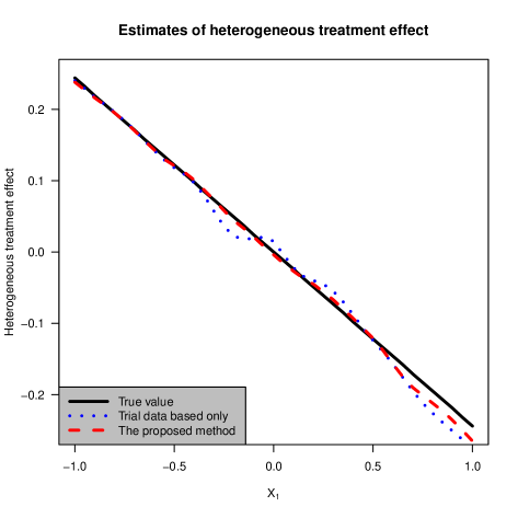
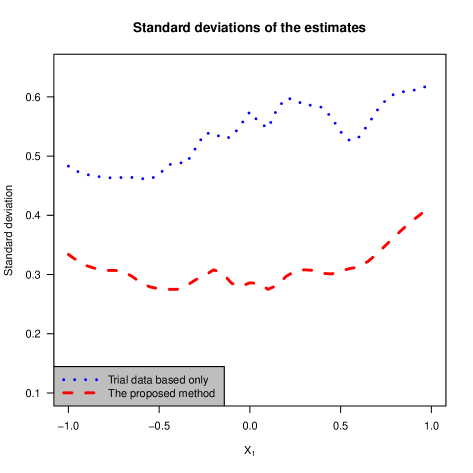
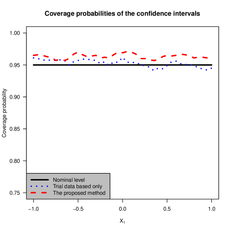
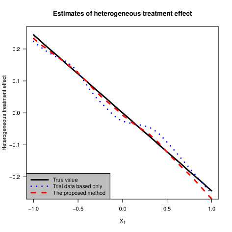
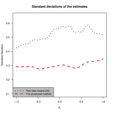
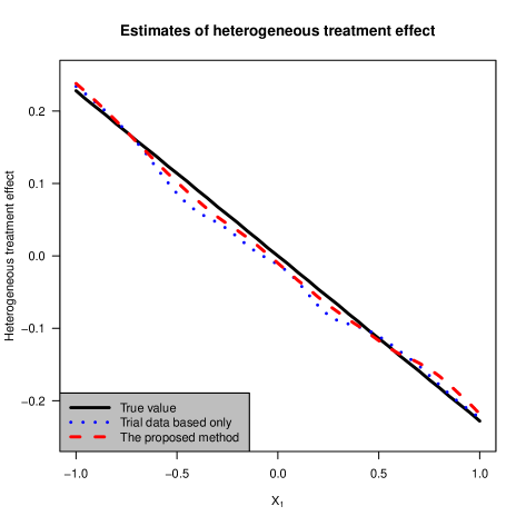
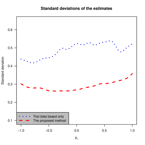
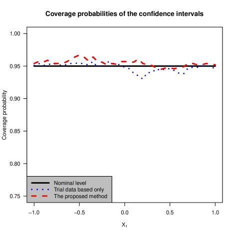
Figure 1: The simulation results with $(n_{1},n_{0})=(500,1000)$ and $X_{2}=0$, spanning from Case 1 to Case 3 (top to bottom). The figure shows HTE estimates, standard deviations and coverage probabilities for two methods: RCTs only (dotted-blue lines) and proposed integrative (dashed-red lines).

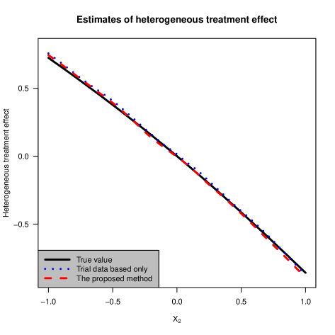
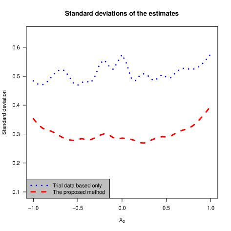
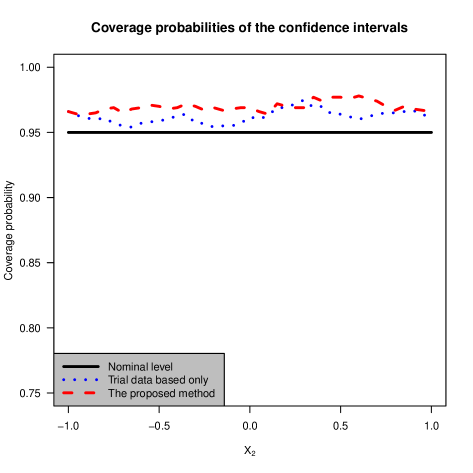
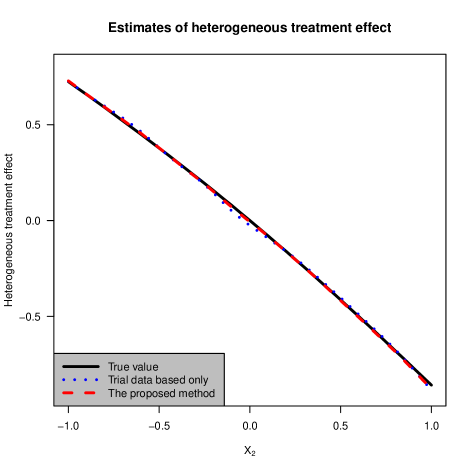
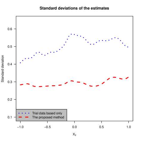
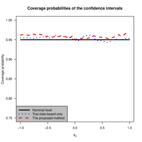
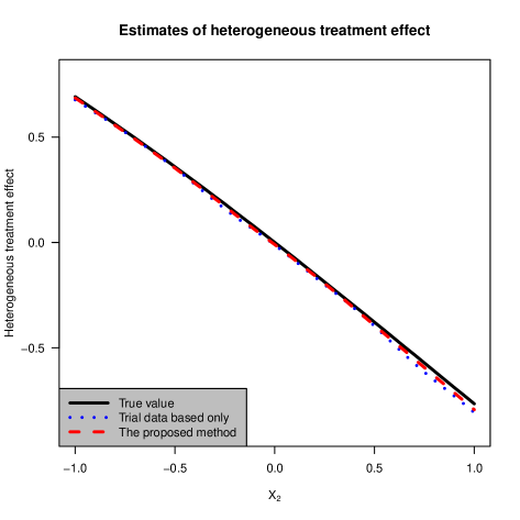
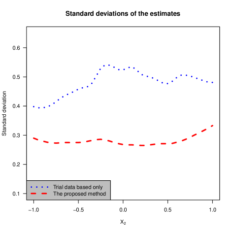
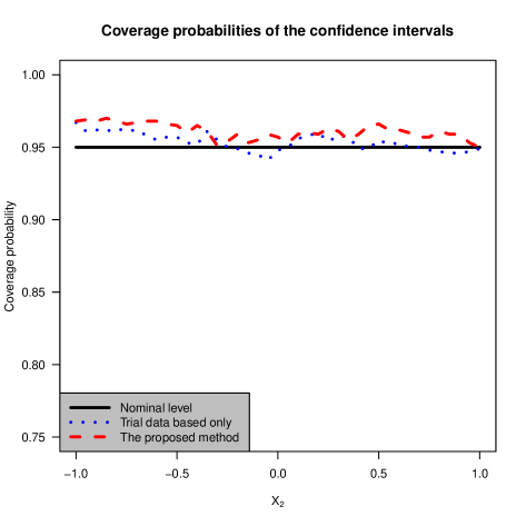
Figure 2: The simulation results with $(n_{1},n_{0})=(500,1000)$ and $X_{1}=0$, spanning from Case 1 to Case 3 (top to bottom). The figure shows HTE estimates, standard deviations and coverage probabilities for two methods: RCTs only (dotted-blue lines) and proposed integrative (dashed-red lines).

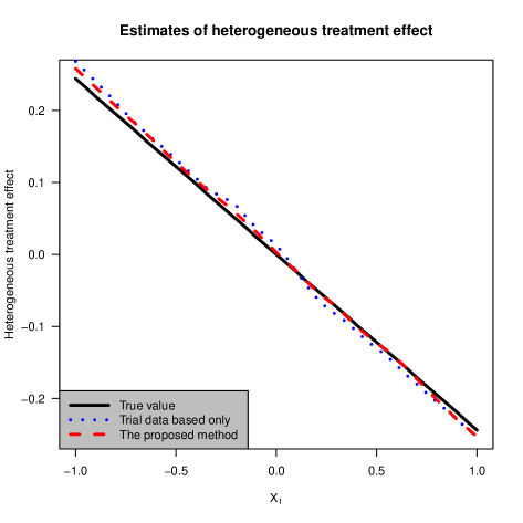
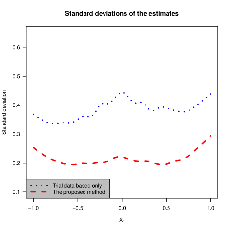
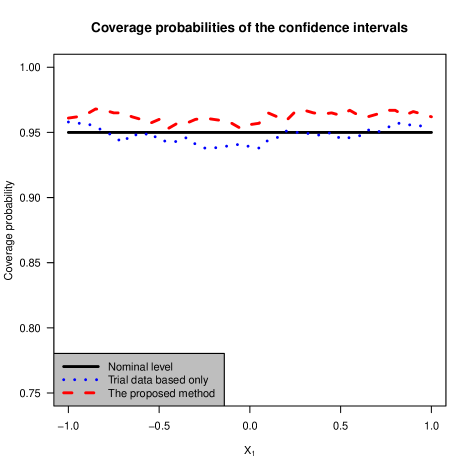
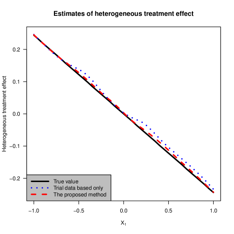
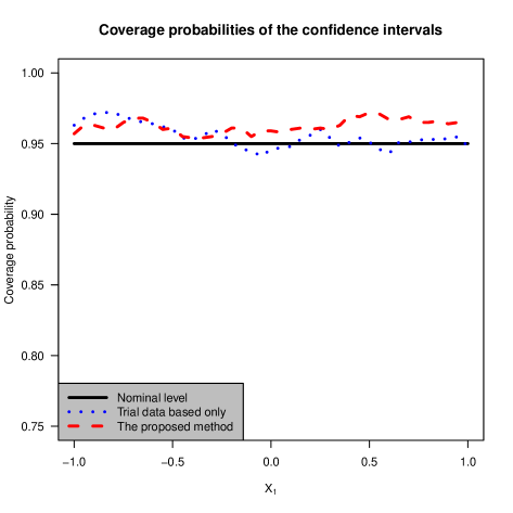
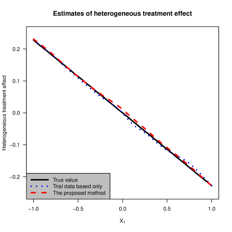
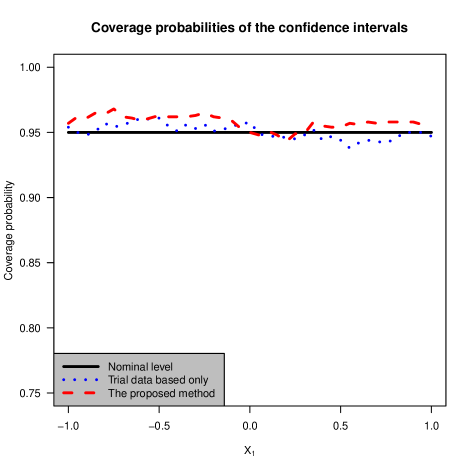
Figure 3: The simulation results with $(n_{1},n_{0})=(1000,2000)$ and $X_{2}=0$, spanning from Case 1 to Case 3 (top to bottom). The figure shows HTE estimates, standard deviations and coverage probabilities for two methods: RCTs only (dotted-blue lines) and proposed integrative (dashed-red lines).

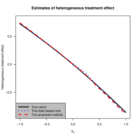
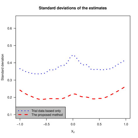
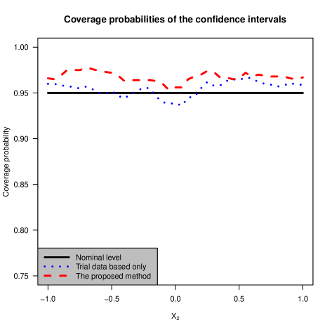
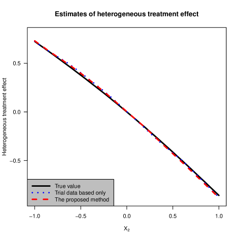
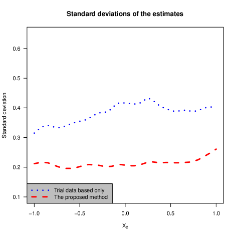
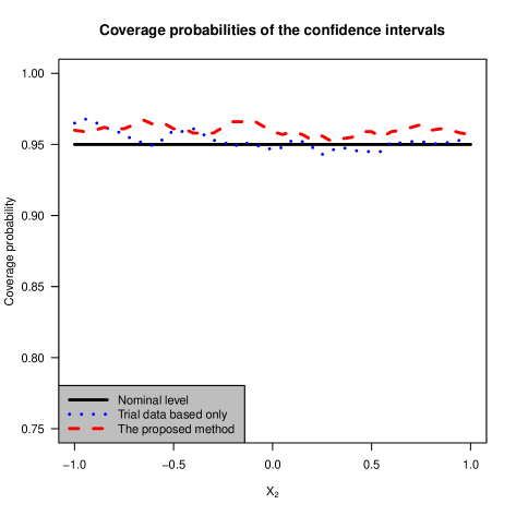
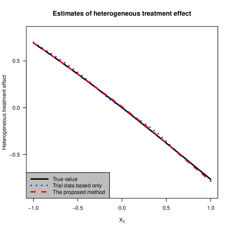
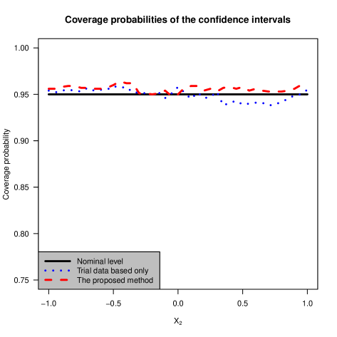
Figure 4: The simulation results with $(n_{1},n_{0})=(1000,2000)$ and $X_{1}=0$, spanning from Case 1 to Case 3 (top to bottom). The figure shows HTE estimates, standard deviations and coverage probabilities for two methods: RCTs only (dotted-blue lines) and proposed integrative (dashed-red lines).

The simulation results are summarized in Figures 1–4. These figures show the empirical mean, standard deviation, and coverage probabilities of the HTE estimates for 1000 replications. Our expectations are met. Both the proposed estimator and the estimate based solely on the RCT data perform well in terms of estimation accuracy and coverage probability, closely aligning with the nominal values. The empirical standard deviations of both the proposed estimator and the estimator based solely on the RCT data significantly decrease when the sample size $(n_{1},n_{0})$ is increased from $(500,1000)$ to $(1000,2000)$. Notably, in all configurations, the empirical standard deviations of the proposed estimators are smaller than those obtained solely from the RCT data. Considering estimation accuracy, coverage probability, and standard deviation together, it is evident that while both methods perform well in terms of accuracy and coverage rate, the proposed method stands out due to its lower standard deviation. The reduced variability of the proposed estimator enhances its reliability, making it a superior choice for estimating the HTE in real-world scenarios. Overall, these findings confirm that the proposed integrative method performs well in finite-sample settings and significantly improves HTE estimation compared to using the RCT data solely.

5.2 Real data application

Due to advances in radiologic technology, the detection rate of early-stage non-small-cell lung cancer is rising. The research community on the treatment of early-stage lung cancer with $\leq$ 2cm tumor had a great interest in evaluating the effect of limited resection relative to lobectomy. Lobectomy is a popular surgical resection in which the entire lobe of the lung where the tumor resides is removed. Limited resection, including wedge and segmental resection, only removes a smaller section of the complicated lobe. Limited resection is known for shorter hospital stays less postoperative complications and better preservation of pulmonary function. CALGB 140503 is a multicenter non-inferiority randomized phase 3 trial in which 697 patients with non-small-cell lung cancer clinically staged as stage 1A with $\leq$ 2cm tumor were randomly assigned to undergo limited resection or lobectomy (Altorki et al., 2023). The results of this trial firmly established that for stage 1A non-small-cell lung cancer patients with tumor size of 2cm or less, limited resection was not inferior to lobectomy concerning overall survival with hazard ratio = 0.95 (90% confidence interval 0.72–1.26) and disease-free survival with hazard ratio = 1.01 (90% confidence interval 0.83–1.24). Further subgroup analysis reveals that patients with older age ($>$ 70 years) tended to have longer disease-free survival and overall survival when receiving limited resection, while patients with larger tumor size (1.5–2cm) tended to benefit more from lobectomy. This leads to a strong interest in exploring treatment effect heterogeneity over age and tumor size. After excluding outliers, we ultimately used data from 694 patients in CALGB 140503.

The National Cancer Database (NCDB) is a clinical oncology database maintained by the American College of Surgeons and it captured 72% of all newly diagnosed lung cancer in the United States. From the NCDB database, we selected a random cohort of 15,000 stage 1A NSCLC patients with $\leq$ 2cm tumor and meet all eligibility criteria of CALGB 140503. The NCDB-only analysis based on multivariable Cox proportional hazards model and propensity score-based methods reveals a significant overall benefit of lobectomy over limited resection, which is contradictory to the findings of CALGB 140503. The benefit of lobectomy over limited resection could be explained by unobserved hidden confounders in the NCDB-only analysis. It has been well documented that surgeons and patients tended to choose limited resection over lobectomy if the patient has bad health status and poor functional respiratory reserve and/or high comorbidity burden (Zhang et al, 2019; Lee and Altorki, 2023). Unfortunately these confounders were not captured in the NCDB database, and these hidden confounders may have inevitably led to biased estimates of the treatment effects. It is of a great interest to illustrate our proposed method to estimate the heterogeneous treatment effect. In particular, we want to examine the precision of the proposed heterogeneous treatment effect estimator for the difference of treatment-specific conditional restricted mean survival times conditional on age and tumor size can be improved by synthesizing information from CALGB 140503 and NCDB cohorts with the latter subject to possible hidden confounders.

Our analysis involves considering the time to death as the survival time and taking age and tumor size as the covariates of interest in a two-dimensional context. The restricted time horizon is set at 3 years. Table 1 displays the descriptive statistics of age and tumor size for the CALGB 140503 and NCDB cohorts. Figure 5 summarizes the results from the trial data-based only approach and the proposed integrative approach. This figure demonstrates that the proposed integrative method provides heterogeneous treatment effect estimates with significantly reduced standard errors and narrower confidence intervals. Additionally, there is a general trend where patients with large tumor size or older age benefit more from lobectomy compared to limited resection, while patients with small tumor size and younger age benefit more from limited resection over lobectomy. Specifically, the left panel in the first row of Figure 5 shows that with a tumor size of 0.7cm (i.e., small tumor size), patients benefit significantly more from limited resection than lobectomy, regardless of age. However, only younger patients ($<$ 57 years) show statistically significant benefits from limited resection over lobectomy. The benefit of limited resection diminishes with moderate tumor size, as shown in the middle panel of the first row of Figure 5 for a tumor size of 1.50cm. Conversely, lobectomy is statistically significantly superior across all age groups when the tumor size is large, as shown in the right panel of the first row of Figure 5 for a tumor size of 1.9cm. The second row of Figure 5 illustrates the treatment effect attributed to tumor size for a specific age group. Generally, the estimates suggest that smaller tumors benefit more from limited resection, whereas larger tumors benefit more from lobectomy. Specifically, younger patients (52 years) with smaller tumors ($<$ 1.4cm) benefit significantly more from limited resection than lobectomy, as shown in the left panel of the second row of Figure5. As tumor size increases, the benefits of lobectomy become more pronounced. From all panels in the second row of Figure 5, it is evident that lobectomy provides statistically significantly greater benefits than limited resection for patients with larger tumor sizes ($>$ 1.6cm) across all age groups. For clarity, the last two rows of Figure 5 illustrate the percentage reduction of standard errors for the corresponding estimates in the first two rows of Figure 5. The analysis results also demonstrate that the proposed integrative method significantly enhances efficiency in real-world applications.

6 Discussion

We proposed an integrative estimator of the HTE by combining evidence from the RCT and the RWD in the presence of right censoring. We avoided the assumption of no biases for the RWD and instead defined a confounding function to account for various biases in the RWD. The proposed method considered the HTE in a fully nonparametric form, making it flexible, model-free, and data-driven, and hence more practical for use in various applications. Our research aimed to increase the efficiency of the HTE estimation by leveraging supplemental information provided by biased RWD, as verified by our numerical studies.

In the introduction, we emphasized the crucial role that the HTE plays in precision medicine. Individualized treatment and precision medicine are frequently used interchangeably, and since the HTE provides guidance regarding which treatment strategy should be adopted, our proposed framework is closely related to the individualized treatment regime, which involves a decision rule that assigns treatments based on patients’ characteristics. Recent studies, such as Chu, Lu, and Yang (2022) and Zhao, Josse, and Yang (2023), have explored the use of data from various sources for the individualized treatment regime. Our research sheds light on the potential application of treatment effects for survival outcomes in precision medicine or individualized treatment, making it a valuable contribution to the field.

Our work also has several limitations that warrant discussion. Firstly, the proposed nonparametric estimators may suffer from boundary effects, which is a common issue in nonparametric statistics. Specifically, point estimates of the HTE in boundary regions could be less accurate than those at interior points due to slower convergence rates of nonparametric estimators around the boundary. Secondly, when using the sieve method to approximate the HTE and the confounding function, the dimensionality of the covariate $\boldsymbol{X}$ should not be high. This restriction limits the practical applications of our method. Although deep learning techniques can expand the applicability of the proposed method to high-dimensional covariates $\boldsymbol{X}$, analyzing the corresponding statistical properties remains challenging. Thirdly, Thirdly, fully nonparametric methods are only suitable for continuous covariates and not for discrete covariates. In fact, the real data analyzed in this paper includes some discrete covariates. Due to these limitations, these covariates cannot be included in the analysis of the HTE. Certainly, parameterizing the impact of discrete covariates and establishing partially linear models for the HTE is feasible. However, analyzing the corresponding theoretical properties is not straightforward and requires more complex proofs. Due to space constraints, this will be left for future research. These limitations should be carefully considered when applying our method in practice.

Supporting Information

Web Appendices referenced in Sections 1, 2, and 4 are available with this paper at the Biometrics website on Wiley Online Library.

Table 1: Distribution of age and tumor size for CALGB 140503 and NCDB Cohorts

	NCDB		CALGB 140503
	Lobectomy	Limited Resection	Lobectomy	Limited Resection
	(N=14505)	(N=3490)	(N=355)	(N=339)
age (years)
Mean (SD)	65.3 (9.64)	67.6 (9.81)	67.1 (8.67)	67.2 (8.73)
Median [Min, Max]	66.0 [38.0, 89.0]	68.0 [38.0,89.0]	67.5 [43.2,88.9]	68.3 [37.8,89.7]
tumor size (cm)
Mean (SD)	1.52 (0.369)	1.40 (0.389)	1.48 (0.355)	1.48 (0.350)
Median [Min, Max]	1.50 [0.400, 2.00]	1.50 [0.400, 2.00]	1.50 [0.600, 2.50]	1.50 [0.400, 2.30]

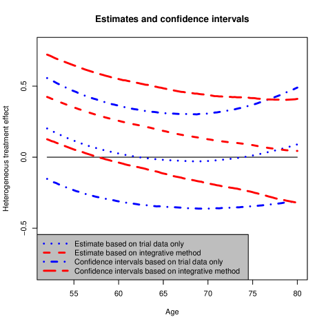
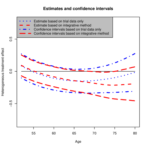
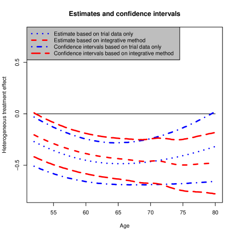
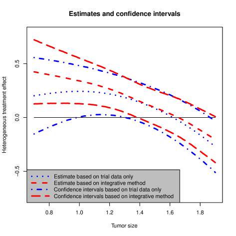
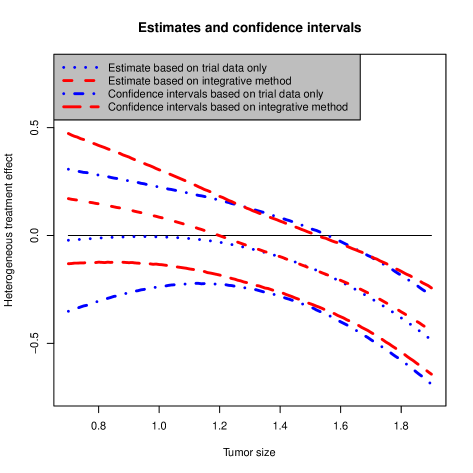
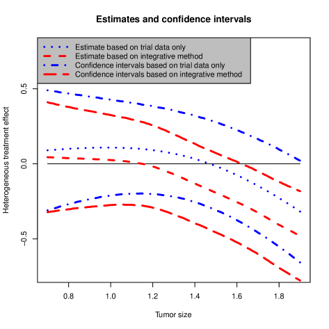
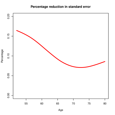
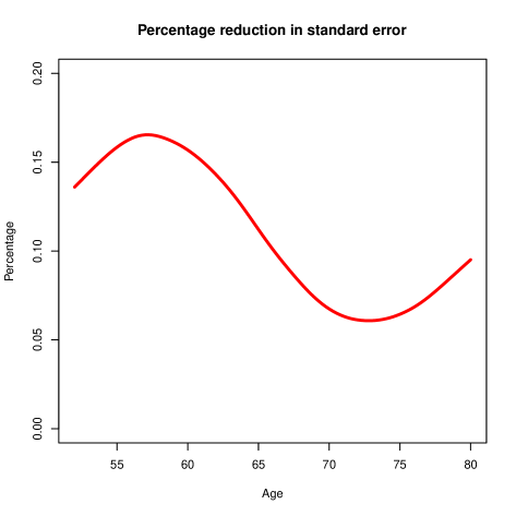
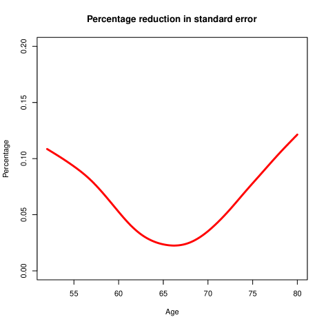
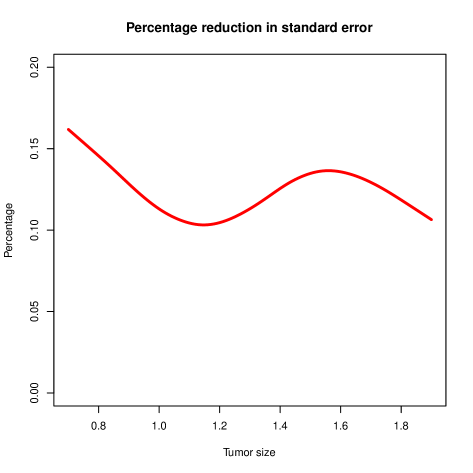
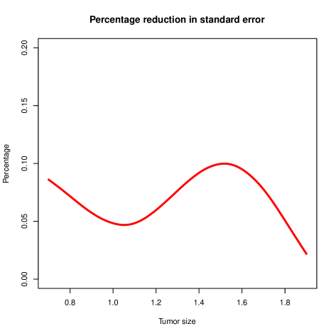
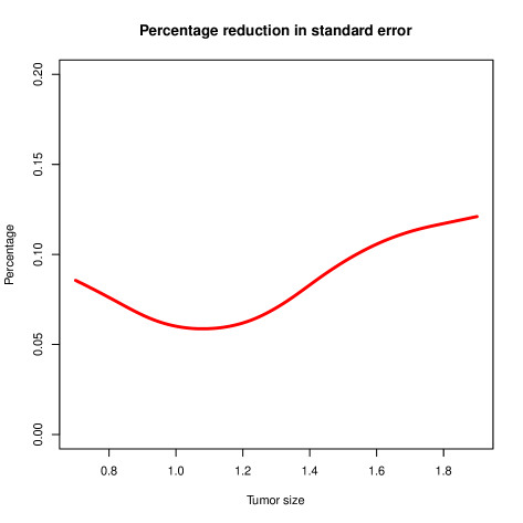
Figure 5: The analysis results in real data, including the HTE as a function of age with tumor sizes 0.7, 1.5, and 1.9cm (first row, from left to right), a function of tumor size with ages 52, 66, and 80 years (second row, from left to right), and the percentage reduction in the standard error of the proposed integrative estimate relative to that based on trial data only (last two rows).

Supplementary

The supplementary material is organized as the following. Web Appendix A presents some additional assumptions for studying the theoretical results of the proposed method. Web Appendix B provides some propositions mentioned in the main paper. Web Appendix C contains some lemmas for proving the theoretical properties. In Web Appendix D, we provide proof of the theoretical properties of the paper.

Let $Z_{1},\ldots,Z_{n^{\prime}}$ be the i.i.d. random variables with probability distribution $\mathbb{Q}$, and $\mathbb{Q}_{n^{\prime}}$ be the empirical measure of these random variables. For a function $f$, we agree on $\mathbb{Q}_{n^{\prime}}f=(n^{\prime})^{-1}\sum_{i=1}^{n^{\prime}}f(Z_{i})$ and $\mathbb{Q}f=\int f(z){\rm d}\mathbb{Q}(z)$. Let $\|f\|_{2}=\{\int f^{2}(z){\rm d}z\}^{1/2}$ and $\|f\|_{\infty}=\sup_{z}|f(z)|$ denote the $L_{2}$ norm and supremum norm of $f$, respectively. Furthermore, for a random function $\widehat{f}(z)=\widehat{f}(z;Z_{1},\ldots,Z_{n^{\prime}})$, which is a measurable function concerning $z$ given observations $Z_{1},\ldots,Z_{n^{\prime}}$, we agree on $E_{r}\{\widehat{f}(Z)\}=\int\widehat{f}(z){\rm d}\mathbb{Q}(z)=E\{f(Z)\}|_{f=\widehat{f}}$ and ${\rm Var}_{r}\{\widehat{f}(Z)\}=\int\widehat{f}^{2}(z){\rm d}\mathbb{Q}(z)-\{\int\widehat{f}(z){\rm d}\mathbb{Q}(z)\}^{2}={\rm Var}\{f(Z)\}|_{f=\widehat{f}}$. Let $\mathbb{P}_{1}$ and $\mathbb{P}_{0}$ denote the probability distribution of $(Y,\Delta,\boldsymbol{X},A,S=1)$ and $(Y,\Delta,\boldsymbol{X},A,S=0)$, respectively. In the following, we use $c_{j}$ to denote a generic positive constant with an appropriate subscript $j$ for $j=0,1,\ldots$, and $c_{j}$ may represent different values in different contexts or lines.

Web Appendix A: Conditions

$\phi_{1}(\cdot),\ldots,\phi_{r_{1}}(\cdot)$ belong to ${\cal H}_{1}$, and $\psi_{1}(\cdot),\ldots,\psi_{r_{0}}(\cdot)$ belong to ${\cal H}_{0}$.

For $f\in{\cal H}_{1}$, $g\in{\cal H}_{0}$, there exist some $f_{n}(\cdot)\in\Phi_{n}$, $g_{n}(\cdot)\in\Psi_{n}$, $\kappa_{1}>\kappa^{\prime}_{1}\geq 0$, and $\kappa_{0}>\kappa^{\prime}_{0}\geq 0$ such that

$$\left\|f_{n}-f\right\|_{\infty} = O(n^{-\kappa_{1}}),\quad\sup_{|k|=m_{1}}\left\|f^{(k)}_{n}-f^{(k)}\right\|_{\infty}=O(n^{-\kappa^{\prime}_{1}}),$$

$$\left\|g_{n}-g\right\|_{\infty} = O(n^{-\kappa_{0}}),\quad\sup_{|k^{\prime}|=m_{0}}\left\|g^{(k^{\prime})}_{n}-g^{(k^{\prime})}\right\|_{\infty}=O(n^{-\kappa^{\prime}_{0}}).$$

$\widehat{D}$ is uniformly bounded and belongs to a class of functions $\mathscr{D}$, and $\{\widehat{\sigma}^{2}_{s}(\boldsymbol{x})\}^{-1}$ is uniformly bounded away from zero and belongs to a class of functions $\mathscr{A}$, such that $\max\{\log N(\epsilon,{\mathscr{D}},\|\cdot\|_{\infty}),\log N(\epsilon,{\mathscr{A}},\|\cdot\|_{\infty})\}<c_{0}\epsilon^{-\upsilon}$ for some constants $c_{0}>0$ and $0<\upsilon<2$, where $N(\epsilon,{\mathscr{D}},\|\cdot\|_{\infty})$ and $N(\epsilon,{\mathscr{A}},\|\cdot\|_{\infty})$ are covering numbers of ${\mathscr{D}}$ and ${\mathscr{A}}$ under supremum norm, and $s=0,1$.

There exist some constants $0<c_{1}<1$ and $c_{2}>0$ such that $c_{1}\leq\widehat{e}(X)\leq 1-c_{1}$, $\widehat{G}_{T}(L\mid\boldsymbol{X},A,S=1)\geq c_{2}$, and $\widehat{G}_{C}(L\mid\boldsymbol{X},A,S=1)\geq c_{2}$.

$c_{3}^{-1}\leq q_{s}(\boldsymbol{x})\leq c_{3}$, where $s=0,1$.

$\sum_{a=0}^{1}\|\Theta_{a}\|_{2}+\|\widehat{e}-e\|_{2}\times\sum_{a=0}^{1}\|\widehat{\mu}_{a}-\mu_{a}\|_{2}=o_{P}(1)$, where

$$\Theta_{A}(\boldsymbol{X}) = \int_{0}^{L}\Bigg{[}G_{T}(t\mid\boldsymbol{X},A,S=1)\int_{0}^{t}\frac{\widehat{G}_{T}(u\mid\boldsymbol{X},A,S=1)-{G}_{T}(u\mid\boldsymbol{X},A,S=1)}{\widehat{G}_{T}(u\mid\boldsymbol{X},A,S=1)}$$

$$\times{\rm d}\left\{\frac{{G}_{C}(u\mid\boldsymbol{X},A,S=1)-\widehat{G}_{C}(u\mid\boldsymbol{X},A,S=1)}{\widehat{G}_{C}(u\mid\boldsymbol{X},A,S=1)}\right\}\Bigg{]}{\rm d}t.$$

$\sum_{a=0}^{1}\|\Theta_{a}\|_{2}+\|\widehat{e}-e\|_{2}\times\sum_{a=0}^{1}\|\widehat{\mu}_{a}-\mu_{a}\|_{2}=O_{P}(\delta_{n})$, where $\delta_{n}=n^{-1/2}\gamma_{1}^{-p/(4m_{1})}+n^{-1/2}\gamma_{0}^{-p/(4m_{0})}+\gamma_{1}^{1/2}+\gamma_{0}^{1/2}$.

$n^{-1/2}\{\gamma_{s}^{(-2m_{s}\upsilon-4p+p\upsilon)/(8m_{s})}+\gamma_{s}^{-(6m_{s}-p)p/(8m_{s}^{2})}\}=o(1)$, where $s=0,1$.

$(n^{-\kappa_{1}}+n^{-\kappa_{0}})=O(\delta_{n})$.

$\sum_{a=0}^{1}\|\Theta_{a}\|_{2}+\|\widehat{e}-e\|_{2}\times\sum_{a=0}^{1}\|\widehat{\mu}_{a}-\mu_{a}\|_{2}=o_{P}(n^{-1/2})$.

$\delta_{n}(\gamma_{1}^{-p/(4m_{1})}+\gamma_{0}^{-p/(4m_{0})})=o(1)$.

$n^{1/2}(n^{-\kappa_{1}}\gamma_{1}^{-1/2}+n^{-\kappa_{0}}\gamma_{0}^{-1/2})\delta_{n}=o(1)$ and $n^{1/2}(n^{-\kappa^{\prime}_{1}}+n^{-\kappa^{\prime}_{0}})\delta_{n}=O(1)$.

$\|\widehat{\sigma}^{2}_{s}-\sigma^{2}_{0s}\|_{\infty}=o_{P}(1)$, where $s=0,1$.

$\|\widehat{D}-D_{0}\|_{\infty}=o_{P}(1)$, where $D_{0}$ is the probability limit of $\widehat{D}$.

$\widehat{\sigma}^{2}(\boldsymbol{X},S)-{\rm Var}_{r}(\widehat{D}\mid\boldsymbol{X},S)=o_{P}(1)$.

There exist some positive constants $\kappa^{*}$ and $\kappa^{\dagger}$ such that $\rho(\boldsymbol{A}^{\rm T}\boldsymbol{A}/n)\asymp n^{-\kappa^{*}}$ and $\rho_{\max}(\boldsymbol{P})=O(n^{\kappa^{\dagger}})$ almost surely, where $\boldsymbol{A}$ and $\boldsymbol{P}$ are defined in the first paragraph of Subsection 6.5, $\rho(\boldsymbol{A}^{\rm T}\boldsymbol{A}/n)$ is the eigenvalues of $\boldsymbol{A}^{\rm T}\boldsymbol{A}/n$ and $\rho_{\max}(\boldsymbol{P})$ is the maximum eigenvalue of $\boldsymbol{P}$.

$(n^{-\kappa_{1}}+n^{-\kappa_{0}})=o(n^{-1/2})$ and $n^{\kappa^{*}+\kappa^{\dagger}}(\gamma_{1}+\gamma_{0})=o(n^{-1/2})$.

Condition Web Appendix A: Conditions ensures that the estimators $\widehat{\tau}_{n}$ and $\widehat{\lambda}_{n}$ are within the subspaces of ${\cal H}_{1}$ and ${\cal H}_{0}$, respectively. Since the theoretical properties are established within the framework of reproducing kernel Hilbert space, this condition is indispensable. However, this condition is mild and easily satisfied. For example, If B-splines or power series with appropriate orders, or reproducing kernels with appropriate smoothness, are selected as the sieve basis, Condition Web Appendix A: Conditions would be met. Condition Web Appendix A: Conditions requires uniform approximation rates to the function and its derivatives. If one chooses the reproducing kernel approximation with some appropriate kernel such as Gaussian kernel, and chooses all the observation data as the knots, then Condition Web Appendix A: Conditions will satisfied with $\kappa_{1}=m_{1}^{\prime}/p$, $\kappa_{1}^{\prime}=(m_{1}^{\prime}-m_{1})/p$, $\kappa_{0}=m_{0}^{\prime}/p$ and $\kappa_{0}^{\prime}=(m_{0}^{\prime}-m_{0})/p$. Additionally, If $f$ and $g$ have continuous $m_{1}^{\prime}$-th and $m_{0}^{\prime}$-th order derivatives, respectively, and further choose B-splines or power series as the sieve basis, and in each dimension, the maximum length between the spline knots is dominated by the inverse of the number of spline knots, then $\|f_{n}-f\|_{\infty}=O(r_{1}^{-m_{1}^{\prime}/p})$, $\sup_{|k|=m_{1}}\|f_{n}^{(k)}-f^{(k)}\|_{\infty}=O(r_{1}^{-(m_{1}^{\prime}-m_{1})/p})$, $\|g_{n}-g\|_{\infty}=O(r_{0}^{-m_{0}^{\prime}/p})$, and $\sup_{|k^{\prime}|=m_{0}}\|g_{n}^{(k^{\prime})}-g^{(k^{\prime})}\|_{\infty}=O(r_{0}^{-(m_{0}^{\prime}-m_{0})/p})$. Moreover, if $r_{1}\asymp n^{\nu_{1}}$ and $r_{0}\asymp n^{\nu_{0}}$, then this condition is satisfied with $\kappa_{1}=m_{1}^{\prime}\nu_{1}/p$, $\kappa_{0}=m_{0}^{\prime}\nu_{0}/p$, $\kappa^{\prime}_{1}=(m_{1}^{\prime}-m_{1})\nu_{1}/p$, and $\kappa^{\prime}_{0}=(m_{0}^{\prime}-m_{0})\nu_{0}/p$. Such a condition appears in Newey (1997). Conditions Web Appendix A: Conditions–Web Appendix A: Conditions are technical. Condition Web Appendix A: Conditions is a regularization condition and controls the complexities of $\widehat{D}$ and $\widehat{\sigma}^{2}_{s}(\boldsymbol{x})$. Especially, Condition Web Appendix A: Conditions implies that $\widehat{D}$ and $\widehat{\sigma}^{2}_{s}(\boldsymbol{x})$ belong to Donsker classes. Condition Web Appendix A: Conditions ensures $\widehat{D}$ to be well defined. It can be easily satisfied for commonly used estimation methods such as some survival models for ${G}_{T}(t\mid\boldsymbol{X},A,S=1)$ and ${G}_{C}(t\mid\boldsymbol{X},A,S=1)$. Condition Web Appendix A: Conditions constitutes a vital prerequisite for Lemma 6.11. Similar or equivalent conditions are also imposed in Cox (1984), Cox (1988), O’Sullivan (1993), and Gu (2013). Under Condition Web Appendix A: Conditions, the square of $L_{2}$ norm is equivalent to $V_{1}$ and $V_{0}$, that is, $c_{4}^{-1}\|f\|_{2}^{2}\leq V_{1}(f,f)\leq c_{4}\|f\|_{2}^{2}$ and $c_{5}^{-1}\|g\|_{2}^{2}\leq V_{0}(g,g)\leq c_{5}\|g\|_{2}^{2}$ for $f\in{\cal H}_{1}$ and $g\in{\cal H}_{0}$.

The remaining conditions are the specific technical conditions required for the theoretical properties in the main paper. Condition Web Appendix A: Conditions is used to derive the robustness of the proposed estimators, as shown in Theorem 1. Conditions Web Appendix A: Conditions–Web Appendix A: Conditions are used for studying the convergence rate of the proposed estimator. The conditions in Remark 1 which presented in the main paper imply that $n^{-1/2}\{\gamma_{s}^{(-2m_{s}\upsilon-4p+p\upsilon)/(8m_{s})}+\gamma_{s}^{-(6m_{s}-p)p/(8m_{s}^{2})}\}\asymp\{n^{-{(2m-p)(2-v)}/(8m+4p)}+n^{-{(2m-p)^{2}}/{(8m^{2}+4mp)}}\}=o(1)$ by $m>p/2$ and $0<\upsilon<2$. Furthermore, if $r_{1}\asymp r_{0}\asymp n^{\nu}$, then Condition Web Appendix A: Conditions can be satisfied by taking $\nu=p/(2m+p)<1/2$. Thus, Conditions Web Appendix A: Conditions–Web Appendix A: Conditions remain valid under the conditions described in Remark 1 which presented in the main paper. Conditions Web Appendix A: Conditions–Web Appendix A: Conditions are imposed for deriving the asymptotic normality. Condition Web Appendix A: Conditions is imposed to ignore the error caused by the nuisance functions. By Theorem 1, various combinations of the convergence rates of $\widehat{G}_{T}$ and $\widehat{G}_{C}$ fulfill this condition. For instance, if parametric models are selected to fit $G_{T}$ and $G_{C}$, and they are correctly specified, then $\sum_{a=0}^{1}\|\Theta_{a}\|_{2}=o_{P}(n^{-1})$. Alternatively, if fully nonparametric estimation is employed for $G_{T}$ and $G_{C}$, Condition Web Appendix A: Conditions would be satisfied under certain smoothness conditions for $G_{T}$ and $G_{C}$. For the conditions outlined in Remark 1 which is presented in the main paper, Condition Web Appendix A: Conditions is automatically satisfied since $m>p/2$. Furthermore, if $m_{1}^{\prime}=m_{0}^{\prime}=m^{\prime}$, $r_{1}\asymp r_{0}\asymp n^{\nu}$, then Condition Web Appendix A: Conditions is fulfilled when $\max\{p/(2m^{\prime}),p^{2}/\{(m^{\prime}-m)(4m+2p)\}\}<\nu<1$. Conditions Web Appendix A: Conditions–Web Appendix A: Conditions enhance pointwise convergence to uniform convergence, but they are rather mild conditions and often easily satisfied by common estimation methods. Uniform convergence is a technical enhancement. It does not significantly limit the applicability of the estimators, rather, it is a reasonable and common condition in both theoretical and practical contexts, especially in the field of survival analysis. Interestingly, here, $\widehat{\sigma}^{2}_{s}(\boldsymbol{X})$ and $\widehat{D}$, as estimators of ${\rm Var}({D}\mid\boldsymbol{X},S=s)$ and $D$, do not need to be consistent. Conditions Web Appendix A: Conditions–Web Appendix A: Conditions are used for studying the efficiency of the proposed estimator. Choosing B-splines as the sieve basis, with the maximum length between spline knots in each dimension dominated by the inverse of the number of knots, ensures that Condition Web Appendix A: Conditions holds with $n^{-\kappa^{*}}\asymp(r_{1}+r_{0})^{-1}$ and $n^{\kappa^{\dagger}}\asymp(r_{1}^{3}+r_{0}^{3})$. Furthermore, if $r_{1}\asymp r_{0}\asymp n^{\nu}$, $\gamma_{1}\asymp\gamma_{0}\asymp n^{-\varsigma}$, and $m_{1}^{\prime}=m_{0}^{\prime}=m^{\prime}$, then Condition Web Appendix A: Conditions holds under the condition $p/(2m^{\prime})<\nu<(2\varsigma-1)/8$. This condition implies that the true functions $\tau_{0}$ and $\lambda_{0}$ should exhibit high smoothness, the number of spline knots should be moderate, and the penalized parameters should be sufficiently small.

Web Appendix B: Propositions

Proposition 6.1

Suppose that Assumptions 1–4 in the paper hold, then

$$E(R\mid\boldsymbol{X},S=1)=\mu_{1}(\boldsymbol{X})-\mu_{0}(\boldsymbol{X})=\tau(\boldsymbol{X}).$$

Proof 6.2

It follows that

$$E(R_{1}\mid A=1,\boldsymbol{X},S=1) = E\{T(1)\wedge L\mid A=1,\boldsymbol{X},S=1\}\frac{1}{e(\boldsymbol{X})}-\frac{1-e(\boldsymbol{X})}{e(\boldsymbol{X})}\mu_{1}(\boldsymbol{X})$$

$$= \mu_{1}(\boldsymbol{X}),$$

$$E({R}_{1}\mid A=0,\boldsymbol{X},S=1) = E\{\mu_{1}(\boldsymbol{X})\mid A=0,\boldsymbol{X},S=1\}=\mu_{1}(\boldsymbol{X}),$$

which implies that $E({R}_{1}\mid\boldsymbol{X},S=1)=\mu_{1}(\boldsymbol{X})$. Similarly, we have $E({R}_{0}\mid\boldsymbol{X},S=1)=\mu_{0}(\boldsymbol{X})$. Combining Assumptions 3–4, we conclude that

$$E(R\mid\boldsymbol{X},S=1) = \mu_{1}(\boldsymbol{X})-\mu_{0}(\boldsymbol{X})$$

$$= E\{T(1)\wedge L\mid A=1,\boldsymbol{X},S=1\}-E\{T(0)\wedge L\mid A=0,\boldsymbol{X},S=1\}$$

$$= E\{T(1)\wedge L\mid\boldsymbol{X},S=1\}-E\{T(0)\wedge L\mid\boldsymbol{X},S=1\}$$

$$= E\{T(1)\wedge L-T(0)\wedge L\mid\boldsymbol{X},S=1\}$$

$$= \tau(\boldsymbol{X}).$$

Hence, we prove Proposition 6.1.

Proposition 6.3

Suppose that Assumptions 5–6 hold, then

$$E\left(\widetilde{T}_{L}\mid\boldsymbol{X},A,S=1\right)=E\left({T}_{L}\mid\boldsymbol{X},A,S=1\right).$$

Proof 6.4

By Assumptions 5 and 6,

$$E\left\{\left.{Y_{L}\widetilde{\Delta}}{G^{-1}_{C}(Y_{L}\mid\boldsymbol{X},A,S=1)}\,\right|\,\boldsymbol{X},A,S=1\right\}$$ (6)

$$= E\left[E\left\{{Y_{L}\widetilde{\Delta}}{G^{-1}_{C}\left(Y_{L}\mid\boldsymbol{X},A,S=1\right)}\,\bigg{|}\,T_{L},\boldsymbol{X},A,S=1\right\}\,\bigg{|}\,\boldsymbol{X},A,S=1\right]$$

$$= E\left[E\left\{{T_{L}\widetilde{\Delta}}{G^{-1}_{C}\left(T_{L}\mid\boldsymbol{X},A,S=1\right)}\,\bigg{|}\,T_{L},\boldsymbol{X},A,S=1\right\}\bigg{|}\boldsymbol{X},A,S=1\right]$$

$$= E\left\{{T_{L}}{G^{-1}_{C}\left(T_{L}\mid\boldsymbol{X},A,S=1\right)}P\left(\widetilde{\Delta}=1\mid T_{L},\boldsymbol{X},A,S=1\right)\,\bigg{|}\,\boldsymbol{X},A,S=1\right\}$$

$$= E\left\{{T_{L}}{G^{-1}_{C}\left(T_{L}\mid\boldsymbol{X},A,S=1\right)}P(C\geq T_{L}\mid T_{L},\boldsymbol{X},A,S=1)\,\bigg{|}\,\boldsymbol{X},A,S=1\right\}$$

$$= E(T_{L}\mid\boldsymbol{X},A,S=1).$$

Thus, it is enough to show that

$$E\left\{\left.\int_{0}^{L}B(t)G^{-1}_{C}(t\mid\boldsymbol{X},A,S=1){\rm d}M_{C}(t)\,\right|\,\boldsymbol{X},A,S=1\right\}=0.$$ (7)

Following Assumption 5, we have

$$E\{N_{C}(t)\mid\boldsymbol{X},A,S=1\} = E\big{[}E\{N_{C}(t)\mid C,\boldsymbol{X},A,S=1\}\mid\boldsymbol{X},A,S=1\big{]}$$

$$= E_{C}\{I(C\leq t)P(C\leq T_{L}\mid C,\boldsymbol{X},A,S=1)\mid\boldsymbol{X},A,S=1\}$$

$$= -\int_{0}^{t}G_{T}(u\mid\boldsymbol{X},A,S=1){\rm d}G_{C}(u\mid\boldsymbol{X},A,S=1).$$

Thus

$$E\left\{\left.\int_{0}^{L}B(t)G^{-1}_{C}(t\mid\boldsymbol{X},A,S=1){\rm d}N_{C}(t)\,\right|\,\boldsymbol{X},A,S=1\right\}$$

$$= -\int_{0}^{L}B(t)G_{T}(t\mid\boldsymbol{X},A,S=1){G^{-1}_{C}(t\mid\boldsymbol{X},A,S=1)}{{\rm d}G_{C}(t\mid\boldsymbol{X},A,S=1)}.$$

On the other hand,

$$E\left\{\left.\int_{0}^{L}B(t){G^{-1}_{C}(t\mid\boldsymbol{X},A,S=1)}{\rm d}Q_{C}(t)\,\right|\,\boldsymbol{X},A,S=1\right\}$$

$$= E\left\{\left.\int_{0}^{L}B(t){G^{-2}_{C}(t\mid\boldsymbol{X},A,S=1)}I(Y_{L}\geq t){{\rm d}G_{C}(t\mid\boldsymbol{X},A,S=1)}\,\right|\,\boldsymbol{X},A,S=1\right\}$$

$$= \int_{0}^{L}B(t){G^{-2}_{C}(t\mid\boldsymbol{X},A,S=1)}P(Y\geq t\mid\boldsymbol{X},A,S=1){{\rm d}G_{C}(t\mid\boldsymbol{X},A,S=1)}$$

$$= \int_{0}^{L}B(t)G_{T}(t\mid\boldsymbol{X},A,S=1){G^{-1}_{C}(t\mid\boldsymbol{X},A,S=1)}{{\rm d}G_{C}(t\mid\boldsymbol{X},A,S=1)},$$

which implies that equation (7) holds. Thus we prove Proposition 6.3.

Web Appendix C: Lemmas

Lemma 6.5

Suppose that Assumptions 1–6 hold, then

$$E_{r}\left(\widehat{T}_{L}-\widetilde{T}_{L}\mid\boldsymbol{X},A,S=1\right)=\Theta_{A}(\boldsymbol{X}),$$

where

$$\widehat{T}_{L}={Y_{L}\widetilde{\Delta}}{\widehat{G}^{-1}_{C}(Y_{L}\mid\boldsymbol{X},A,S=1)}-\int_{0}^{L}\widehat{B}(t)\widehat{G}^{-1}_{C}(t\mid\boldsymbol{X},A,S=1){\rm d}\widehat{M}_{C}(t),$$

is the corresponding estimator of $\widetilde{T}_{L}$, $\widehat{B}(t)=t+{\int_{t}^{L}\widehat{G}_{T}(u\mid\boldsymbol{X},A,S=1){\rm d}u}/{\widehat{G}_{T}(t\mid\boldsymbol{X},A,S=1)}$ and $\widehat{M}_{C}(t)=N_{C}(t)+\widehat{Q}_{C}(t)$ with $\widehat{Q}_{C}(t)=\int_{0}^{t}I(Y_{L}\geq u)\widehat{G}^{-1}_{C}(u\mid\boldsymbol{X},A,S=1){\rm d}\widehat{G}_{C}(u\mid\boldsymbol{X},A,S=1)$, and

$$\Theta_{A}(\boldsymbol{X}) = \int_{0}^{L}\Bigg{[}G_{T}(t\mid\boldsymbol{X},A,S=1)\int_{0}^{t}\frac{\widehat{G}_{T}(u\mid\boldsymbol{X},A,S=1)-{G}_{T}(u\mid\boldsymbol{X},A,S=1)}{\widehat{G}_{T}(u\mid\boldsymbol{X},A,S=1)}$$

$$\times{\rm d}\left\{\frac{{G}_{C}(u\mid\boldsymbol{X},A,S=1)-\widehat{G}_{C}(u\mid\boldsymbol{X},A,S=1)}{\widehat{G}_{C}(u\mid\boldsymbol{X},A,S=1)}\right\}\Bigg{]}{\rm d}t.$$

Proof 6.6

By the definition of $E_{r}$ and Proposition 6.3,

$$E_{r}\left(\widetilde{T}_{L}\mid\boldsymbol{X},A,S=1\right)=E\left(\widetilde{T}_{L}\mid\boldsymbol{X},A,S=1\right) = E\left(T_{L}\mid\boldsymbol{X},A,S=1\right)$$ (8)

$$= \int_{0}^{L}G_{T}(t\mid\boldsymbol{X},A,S=1){\rm d}t.$$

Mimicking the proof of equation (6), we have

$$E_{r}\left\{\left.{Y_{L}\widetilde{\Delta}}{\widehat{G}^{-1}_{C}(Y_{L}\mid\boldsymbol{X},A,S=1)}\,\right|\,\boldsymbol{X},A,S=1\right\}$$ (9)

$$= E_{r}\left\{\left.T_{L}{G_{C}(T_{L}\mid\boldsymbol{X},A,S=1)}{\widehat{G}^{-1}_{C}(T_{L}\mid\boldsymbol{X},A,S=1)}\,\right|\,\boldsymbol{X},A,S=1\right\}$$

$$= \int_{0}^{L}G_{T}(t\mid\boldsymbol{X},A,S=1)G_{C}(t\mid\boldsymbol{X},A,S=1)\widehat{G}^{-1}_{C}(t\mid\boldsymbol{X},A,S=1){\rm d}t$$

$$+\int_{0}^{L}tG_{T}(t\mid\boldsymbol{X},A,S=1){\rm d}\left\{G_{C}(t\mid\boldsymbol{X},A,S=1)\widehat{G}^{-1}_{C}(t\mid\boldsymbol{X},A,S=1)\right\}.$$

Furthermore,

$$E_{r}\left\{\int_{0}^{L}\widehat{B}(t)\widehat{G}^{-1}_{C}(t\mid\boldsymbol{X},A,S=1){\rm d}\widehat{M}_{C}(t)\,\big{|}\,\boldsymbol{X},A,S=1\right\}$$ (10)

$$= -E_{r}\left\{\int_{0}^{L}\widehat{B}(t)\widehat{G}^{-1}_{C}(t\mid\boldsymbol{X},A,S=1){\rm d}{Q}_{C}(t)\,\big{|}\,\boldsymbol{X},A,S=1\right\}$$

$$+E_{r}\left\{\int_{0}^{L}\widehat{B}(t)\widehat{G}^{-1}_{C}(t\mid\boldsymbol{X},A,S=1){\rm d}\widehat{Q}_{C}(t)\,\big{|}\,\boldsymbol{X},A,S=1\right\}$$

$$= -E_{r}\bigg{\{}\int_{0}^{L}\widehat{B}(t)\widehat{G}^{-1}_{C}(t\mid\boldsymbol{X},A,S=1){G}^{-1}_{C}(t\mid\boldsymbol{X},A,S=1)$$

$$\times I(Y_{L}\geq t){\rm d}{G}_{C}(t\mid\boldsymbol{X},A,S=1)\,\big{|}\,\boldsymbol{X},A,S=1\bigg{\}}$$

$$+E_{r}\bigg{\{}\int_{0}^{L}\widehat{B}(t)\widehat{G}^{-1}_{C}(t\mid\boldsymbol{X},A,S=1)\widehat{G}^{-1}_{C}(t\mid\boldsymbol{X},A,S=1)$$

$$\times I(Y_{L}\geq t){\rm d}\widehat{G}_{C}(t\mid\boldsymbol{X},A,S=1)\,\big{|}\,\boldsymbol{X},A,S=1\bigg{\}}$$

$$= \int_{0}^{L}\widehat{B}(t)G_{T}(t\mid\boldsymbol{X},A,S=1){\rm d}\left\{{G}^{-1}_{C}(t\mid\boldsymbol{X},A,S=1)\widehat{G}^{-1}_{C}(t\mid\boldsymbol{X},A,S=1)\right\}$$

$$= \int_{0}^{L}tG_{T}(t\mid\boldsymbol{X},A,S=1){\rm d}\left\{G_{C}(t\mid\boldsymbol{X},A,S=1)\widehat{G}^{-1}_{C}(t\mid\boldsymbol{X},A,S=1)\right\}$$

$$+\int_{0}^{L}G_{T}(t\mid\boldsymbol{X},A,S=1)\bigg{[}\int_{0}^{t}G_{T}(u\mid\boldsymbol{X},A,S=1)$$

$$\times\widehat{G}^{-1}_{T}(u\mid\boldsymbol{X},A,S=1){\rm d}\left\{G_{C}(u\mid\boldsymbol{X},A,S=1)\widehat{G}^{-1}_{C}(u\mid\boldsymbol{X},A,S=1)\right\}\bigg{]}{\rm d}t,$$

by using the Fubini Theorem.

Combining equations (8)–(10), we have

$$E_{r}\left(\widehat{T}_{L}-\widetilde{T}_{L}\mid\boldsymbol{X},A,S=1\right)$$

$$= \int_{0}^{L}G_{T}(t\mid\boldsymbol{X},A,S=1)\Bigg{[}\frac{{G}_{C}(u\mid\boldsymbol{X},A,S=1)-\widehat{G}_{C}(u\mid\boldsymbol{X},A,S=1)}{\widehat{G}_{C}(u\mid\boldsymbol{X},A,S=1)}$$

$$-\int_{0}^{t}\frac{G_{T}(u\mid\boldsymbol{X},A,S=1)}{\widehat{G}_{T}(u\mid\boldsymbol{X},A,S=1)}{\rm d}\left\{\frac{G_{C}(u\mid\boldsymbol{X},A,S=1)}{\widehat{G}_{C}(u\mid\boldsymbol{X},A,S=1)}\right\}\Bigg{]}{\rm d}t$$

$$= \int_{0}^{L}G_{T}(t\mid\boldsymbol{X},A,S=1)\Bigg{[}\int_{0}^{t}\frac{\widehat{G}_{T}(u\mid\boldsymbol{X},A,S=1)-{G}_{T}(u\mid\boldsymbol{X},A,S=1)}{\widehat{G}_{T}(u\mid\boldsymbol{X},A,S=1)}$$

$$\times{\rm d}\left\{\frac{{G}_{C}(u\mid\boldsymbol{X},A,S=1)-\widehat{G}_{C}(u\mid\boldsymbol{X},A,S=1)}{\widehat{G}_{C}(u\mid\boldsymbol{X},A,S=1)}\right\}\Bigg{]}{\rm d}t$$

$$= \Theta_{A}(\boldsymbol{X}).$$

Thus, we complete the proof of Lemma 6.5.

Lemma 6.7

Suppose that Assumptions 1–6 hold, then

$$E_{r}\left(\widehat{D}-D\mid\boldsymbol{X},S=1\right)=\Gamma_{1}(\boldsymbol{X})+\Gamma_{2}(\boldsymbol{X}),$$

where

$$\Gamma_{1}(\boldsymbol{X}) = \sum_{a=0}^{1}\frac{\left\{\widehat{e}(\boldsymbol{X})-e(\boldsymbol{X})\right\}\left\{\widehat{\mu}_{a}(\boldsymbol{X})-\mu_{a}(\boldsymbol{X})\right\}}{a\widehat{e}(\boldsymbol{X})+(1-a)\left\{1-\widehat{e}(\boldsymbol{X})\right\}},$$

$$\Gamma_{2}(\boldsymbol{X}) = \sum_{a=0}^{1}\frac{a{e}(\boldsymbol{X})+(a-1)\{1-{e}(\boldsymbol{X})\}}{a\widehat{e}(\boldsymbol{X})+(1-a)\left\{1-\widehat{e}(\boldsymbol{X})\right\}}\Theta_{a}(\boldsymbol{X}).$$

Proof 6.8

For $S=1$, we have $\widehat{D}-D=\widehat{R}-\widetilde{R}$. Rewrite $\widehat{R}$ as

$$\widehat{R}=\frac{A-\widehat{e}(\boldsymbol{X})}{\widehat{e}(\boldsymbol{X})\{1-\widehat{e}(\boldsymbol{X})\}}\left\{\widehat{T}_{L}-\widehat{\mu}_{A}(\boldsymbol{X})\right\}+\widehat{\mu}_{1}(\boldsymbol{X})-\widehat{\mu}_{0}(\boldsymbol{X}),$$

where $\widehat{\mu}_{A}(\boldsymbol{X})=A\,\widehat{\mu}_{1}(\boldsymbol{X})+(1-A)\,\widehat{\mu}_{0}(\boldsymbol{X})$. Using Proposition 6.3 and Lemma 6.5, we have

$$E_{r}\left(\widehat{R}\mid\boldsymbol{X},S=1\right)$$

$$= E_{r}\left[\frac{A-\widehat{e}(\boldsymbol{X})}{\widehat{e}(\boldsymbol{X})\{1-\widehat{e}(\boldsymbol{X})\}}\left\{\widehat{T}_{L}-\widehat{\mu}_{A}(\boldsymbol{X})\right\}+\widehat{\mu}_{1}(\boldsymbol{X})-\widehat{\mu}_{0}(\boldsymbol{X})\,\bigg{|}\,\boldsymbol{X},S=1\right]$$

$$+E_{r}\left[\frac{A-\widehat{e}(\boldsymbol{X})}{\widehat{e}(\boldsymbol{X})\{1-\widehat{e}(\boldsymbol{X})\}}\left(\widehat{T}_{L}-\widetilde{T}_{L}\right)\,\bigg{|}\,\boldsymbol{X},S=1\right]$$

$$= E_{r}\left[\frac{A-\widehat{e}(\boldsymbol{X})}{\widehat{e}(\boldsymbol{X})\{1-\widehat{e}(\boldsymbol{X})\}}\left\{\widetilde{T}_{L}-\widehat{\mu}_{A}(\boldsymbol{X})\right\}\,\bigg{|}\,\boldsymbol{X},S=1\right]+\widehat{\mu}_{1}(\boldsymbol{X})-\widehat{\mu}_{0}(\boldsymbol{X})$$

$$+E_{r}\left(E_{r}\left[\frac{A-\widehat{e}(\boldsymbol{X})}{\widehat{e}(\boldsymbol{X})\{1-\widehat{e}(\boldsymbol{X})\}}\left(\widehat{T}_{L}-\widetilde{T}_{L}\right)\,\bigg{|}\,\boldsymbol{X},A,S=1\right]\,\bigg{|}\,\boldsymbol{X},S=1\right),$$

$$= \frac{e(\boldsymbol{X})}{\widehat{e}(\boldsymbol{X})}\left\{\mu_{1}(\boldsymbol{X})-\widehat{\mu}_{1}(\boldsymbol{X})\right\}-\frac{1-e(\boldsymbol{X})}{1-\widehat{e}(\boldsymbol{X})}\left\{\mu_{0}(\boldsymbol{X})-\widehat{\mu}_{0}(\boldsymbol{X})\right\}$$

$$+\widehat{\mu}_{1}(\boldsymbol{X})-\widehat{\mu}_{0}(\boldsymbol{X})+\Gamma_{2}(\boldsymbol{X}),$$

combined with Proposition 6.1,

$$E_{r}\left(\widehat{R}-\widetilde{R}\mid\boldsymbol{X},S=1\right)$$

$$= \frac{\widehat{e}(\boldsymbol{X})-e(\boldsymbol{X})}{\widehat{e}(\boldsymbol{X})}\left\{\widehat{\mu}_{1}(\boldsymbol{X})-\mu_{1}(\boldsymbol{X})\right\}+\frac{\widehat{e}(\boldsymbol{X})-e(\boldsymbol{X})}{1-\widehat{e}(\boldsymbol{X})}\left\{\widehat{\mu}_{0}(\boldsymbol{X})-\mu_{0}(\boldsymbol{X})\right\}+\Gamma_{2}(\boldsymbol{X})$$

$$= \Gamma_{1}(\boldsymbol{X})+\Gamma_{2}(\boldsymbol{X}),$$

which proves Lemma 6.7.

Lemma 6.9

Let $\pi_{1}(\boldsymbol{x})$ and $\pi_{0}(\boldsymbol{x})$ be some functions which are uniformly bounded away from zero, $\varpi$ be some positive constant such that $0<\varpi<1$, and

$$\ell^{\dagger}(f,g)=\varpi\int_{\Omega}\pi_{1}(\boldsymbol{x})f^{2}(\boldsymbol{x})q_{1}(\boldsymbol{x}){\rm d}\boldsymbol{x}+(1-\varpi)\int_{\Omega}\pi_{0}(\boldsymbol{x})\{f(\boldsymbol{x})+g(\boldsymbol{x})\}^{2}q_{0}(\boldsymbol{x}){\rm d}\boldsymbol{x},$$

where $(f,g)\in{\cal H}$. Suppose that Condition Web Appendix A: Conditions holds, then there exists some positive constant $c_{0}$ such that

$$\ell^{\dagger}(f,g)\geq c_{0}\{V_{1}(f,f)+V_{0}(g,g)\},$$

for all $(f,g)\in{\cal H}$.

Proof 6.10

It follows from Condition Web Appendix A: Conditions and Hölder inequality that

$$\ell^{\dagger}(f,g) = \varpi\int_{\Omega}\pi_{1}(\boldsymbol{x})f^{2}(\boldsymbol{x})q_{1}(\boldsymbol{x}){\rm d}\boldsymbol{x}+(1-\varpi)\int_{\Omega}\pi_{0}(\boldsymbol{x})\{f(\boldsymbol{x})+g(\boldsymbol{x})\}^{2}q_{0}(\boldsymbol{x}){\rm d}\boldsymbol{x}$$

$$\geq c_{1}\left\{\int_{\Omega}f^{2}(\boldsymbol{x}){\rm d}\boldsymbol{x}+\int_{\Omega}\{f(\boldsymbol{x})+g(\boldsymbol{x})\}^{2}{\rm d}\boldsymbol{x}\right\}$$

$$\geq c_{1}\left[2\int_{\Omega}f^{2}(\boldsymbol{x}){\rm d}\boldsymbol{x}+\int_{\Omega}g^{2}(\boldsymbol{x}){\rm d}\boldsymbol{x}-2\left\{\int_{\Omega}f^{2}(\boldsymbol{x}){\rm d}\boldsymbol{x}\right\}^{1/2}\left\{\int_{\Omega}g^{2}(\boldsymbol{x}){\rm d}\boldsymbol{x}\right\}^{1/2}\right],$$

and the equality in the last inequality holds if and only if there exists a non-negative function $\varsigma(\boldsymbol{x})$ which is constant almost everywhere in Lebesgue measure such that $g(\boldsymbol{x})=-\varsigma(\boldsymbol{x})f(\boldsymbol{x})=-\varsigma f(\boldsymbol{x})$.

For $\boldsymbol{h}=(f,g)\in{\cal H}$ and $\widetilde{\boldsymbol{h}}=(\widetilde{f},\widetilde{g})\in{\cal H}$, define the $L_{2}$ norm on ${\cal H}$ as $\|\boldsymbol{h}\|_{2}=\left(\|f\|_{2}^{2}+\|g\|_{2}^{2}\right)^{1/2}$ and a bilinear functional $B^{\dagger}:{\cal H}\times{\cal H}\rightarrow\mathbb{R}$ as

$$B^{\dagger}[\boldsymbol{h}][\widetilde{\boldsymbol{h}}] = \varpi\int_{\Omega}\pi_{1}(\boldsymbol{x})f(\boldsymbol{x})\widetilde{f}(\boldsymbol{x})q_{1}(\boldsymbol{x}){\rm d}\boldsymbol{x}$$

$$+(1-\varpi)\int_{\Omega}\pi_{0}(\boldsymbol{x})\{f(\boldsymbol{x})+g(\boldsymbol{x})\}\{\widetilde{f}(\boldsymbol{x})+\widetilde{g}(\boldsymbol{x})\}q_{0}(\boldsymbol{x}){\rm d}\boldsymbol{x}.$$

Obviously, $\ell^{\dagger}(f,g)=B^{\dagger}[\boldsymbol{h}][\boldsymbol{h}]$. Then

$$\inf_{\|\boldsymbol{h}\|_{2}=1}B^{\dagger}[\boldsymbol{h}][{\boldsymbol{h}}] = \inf_{\|f\|_{2}^{2}+\|g\|_{2}^{2}=1}\ell^{\dagger}(f,g)$$

$$\geq \inf_{\|f\|_{2}^{2}+\|g\|_{2}^{2}=1,g=-\varsigma f}c_{1}\left\{\int_{\Omega}f^{2}(\boldsymbol{x}){\rm d}\boldsymbol{x}+\int_{\Omega}\{f(\boldsymbol{x})+g(\boldsymbol{x})\}^{2}{\rm d}\boldsymbol{x}\right\}$$

$$= c_{1}\inf_{\varsigma>0}\left(1+\frac{1-2\varsigma}{1+\varsigma^{2}}\right)$$

$$= \frac{\sqrt{5}-1}{\sqrt{5}+1}c_{1},$$

which implies that

$$\ell^{{\dagger}}(f,g)=B^{\dagger}[\boldsymbol{h}][\boldsymbol{h}] \geq \left(\inf_{\|\boldsymbol{h}\|_{2}=1}B^{\dagger}[\boldsymbol{h}][\boldsymbol{h}]\right)\cdot\|\boldsymbol{h}\|_{2}^{2}$$

$$\geq \frac{\sqrt{5}-1}{\sqrt{5}+1}c_{1}\|\boldsymbol{h}\|_{2}^{2}$$

$$= \frac{\sqrt{5}-1}{\sqrt{5}+1}c_{1}\left(\|f\|_{2}^{2}+\|g\|_{2}^{2}\right)$$

$$\geq \frac{\sqrt{5}-1}{\sqrt{5}+1}c_{1}\left\{c_{2}V_{1}(f,f)+c_{3}V_{0}(g,g)\right\}$$

$$\geq c_{4}\left\{V_{1}(f,f)+V_{0}(g,g)\right\},$$

by using Condition Web Appendix A: Conditions. Thus, we proves Lemma 6.9.

Lemma 6.11

Suppose that Condition Web Appendix A: Conditions holds, then

1. There exist a sequence of eigenfunctions $\varphi_{1\mu}\in{\cal H}_{1}$ ($\mu\in\mathbb{N}$) satisfying $\sup_{\mu\in\mathbb{N}}\|{\varphi_{1\mu}}\|_{\infty}\leq c_{1}$ and the corresponding non-decreasing sequence of eigenvalues $\rho_{1\mu}$ ($\mu\in\mathbb{N}$) such that $V_{1}(\varphi_{1\mu},\varphi_{1\mu^{\prime}})=\delta_{\mu\mu^{\prime}}$ and $J_{1}(\varphi_{1\mu},\varphi_{1\mu^{\prime}})=\rho_{1\mu}\delta_{\mu\mu^{\prime}}$, where $\delta_{\mu\mu^{\prime}}$ is the Kronecker’s delta and $\mathbb{N}=\{0,1,2,\ldots\}$. Furthermore, there exist a sequence of eigenfunctions $\varphi_{0\mu}\in{\cal H}_{0}$ ($\mu\in\mathbb{N}$) satisfying $\sup_{\mu\in\mathbb{N}}\|{\varphi_{0\mu}}\|_{\infty}\leq c_{0}$ and the corresponding non-decreasing sequence of eigenvalues $\rho_{0\mu}$ ($\mu\in\mathbb{N}$) such that $V_{0}(\varphi_{0\mu},\varphi_{0\mu^{\prime}})=\delta_{\mu\mu^{\prime}}$ and $J_{0}(\varphi_{0\mu},\varphi_{0\mu^{\prime}})=\rho_{0\mu}\delta_{\mu\mu^{\prime}}$.

2. $\rho_{1\mu}\asymp\mu^{2m_{1}/p}$ and $\rho_{0\mu}\asymp\mu^{2m_{0}/p}$ for sufficiently large $\mu$.

3. $f=\sum_{\mu}V_{1}(f,\varphi_{1\mu})\varphi_{1\mu}$ and $g=\sum_{\mu}V_{0}(g,\varphi_{0\mu})\varphi_{0\mu}$ for $f\in{\cal H}_{1}$ and $g\in{\cal H}_{0}$, where $\sum_{\mu}$ denotes the sum over $\mathbb{N}=\{0,1,2,\ldots\}$.

The conclusion of Lemma 6.11 appears in many literature, see Cox (1984) on page 799, Cox (1988) on page 699, O’Sullivan (1993) on page 132, Gu (2013) on page 322, and thus we omit the proof.

Lemma 6.12

Suppose that Condition Web Appendix A: Conditions holds, then for $f\in{\cal H}_{1},g\in{\cal H}_{0}$, and $\boldsymbol{x}\in\Omega$, we have

$$K_{1\boldsymbol{x}}(\cdot) = \sum_{\mu}\frac{\varphi_{1\mu}(\boldsymbol{x})}{1+\gamma_{1}\rho_{1\mu}}\varphi_{1\mu}(\cdot),\quad W_{\gamma_{1}}\varphi_{1\mu}(\cdot)=\frac{\gamma_{1}\rho_{1\mu}}{1+\gamma_{1}\rho_{1\mu}}\varphi_{1\mu}(\cdot),$$

$$\|f\|_{{\cal H}_{1}}^{2} = \sum_{\mu}|V_{1}(f,\varphi_{1\mu})|^{2}(1+\gamma_{1}\rho_{1\mu})=\sum_{\mu}\frac{|\langle f,\varphi_{1\mu}\rangle_{{\cal H}_{1}}|^{2}}{1+\gamma_{1}\rho_{1\mu}},$$

and

$$K_{0\boldsymbol{x}}(\cdot) = \sum_{\mu}\frac{\varphi_{0\mu}(\boldsymbol{x})}{1+\gamma_{0}\rho_{0\mu}}\varphi_{0\mu}(\cdot),\quad W_{\gamma_{0}}\varphi_{0\mu}(\cdot)=\frac{\gamma_{0}\rho_{0\mu}}{1+\gamma_{0}\rho_{0\mu}}\varphi_{0\mu}(\cdot),$$

$$\|g\|_{{\cal H}_{0}}^{2} = \sum_{\mu}|V_{0}(g,\varphi_{0\mu})|^{2}(1+\gamma_{0}\rho_{0\mu})=\sum_{\mu}\frac{|\langle g,\varphi_{0\mu}\rangle_{{\cal H}_{0}}|^{2}}{1+\gamma_{0}\rho_{0\mu}}.$$

Lemma 6.13

Suppose that Condition Web Appendix A: Conditions holds, then for every $\boldsymbol{x}\in\Omega$, we have

$$\|K_{1\boldsymbol{x}}\|_{{\cal H}_{1}}\leq\widetilde{c}_{1}\gamma_{1}^{-p/(4m_{1})},\quad\|K_{0\boldsymbol{x}}\|_{{\cal H}_{0}}\leq\widetilde{c}_{0}\gamma_{0}^{-p/(4m_{0})},$$

where $\widetilde{c}_{1}$ and $\widetilde{c}_{0}$ do not depend on the choice of $\boldsymbol{x}$. Furthermore,

$$\|f\|_{\infty}\leq\widetilde{c}_{1}\gamma_{1}^{-p/(4m_{1})}\|f\|_{{\cal H}_{1}},\quad\|g\|_{\infty}\leq\widetilde{c}_{0}\gamma_{0}^{-p/(4m_{0})}\|g\|_{{\cal H}_{0}},$$

for every $f\in{\cal H}_{1}$ and $g\in{\cal H}_{0}$.

Lemmas 6.12 and 6.13 are similar to Proposition 2.1 and Lemma 3.1 in Shang and Cheng (2013), and Lemma 0.1 and Lemma 0.2 in the supplementary material of Liu et al. (2020). The proofs essentially proceed along the lines of these literature and are trivial and omitted for the sake of brevity.

Lemma 6.14

Suppose that Condition Web Appendix A: Conditions holds, then for $f\in{\cal H}_{1}$ and $g\in{\cal H}_{0}$ such that $J_{1}(f,f)\leq c_{1}$ and $J_{0}(g,g)\leq c_{0}$, we have

$$\|W_{\gamma_{1}}f\|_{{\cal H}_{1}}=o(\gamma_{1}^{1/2}),\quad\|W_{\gamma_{0}}g\|_{{\cal H}_{0}}=o(\gamma_{0}^{1/2}).$$

Proof 6.15

It follows from Lemmas 6.11 and 6.12 that

$$\|W_{\gamma_{1}}f\|_{{\cal H}_{1}}^{2} = \sum_{\mu}|V_{1}(W_{\gamma_{1}}f,\varphi_{1\mu})|^{2}(1+\gamma_{1}\rho_{1\mu})$$

$$= \sum_{\mu}\left|V_{1}\left(\sum_{\mu^{\prime}}V_{1}(f,\varphi_{1\mu^{\prime}})W_{\gamma_{1}}\varphi_{1\mu^{\prime}},\varphi_{1\mu}\right)\right|^{2}(1+\gamma_{1}\rho_{1\mu})$$

$$= \sum_{\mu}|V_{1}(f,\varphi_{1\mu})|^{2}\left(\frac{\gamma_{1}\rho_{1\mu}}{1+\gamma_{1}\rho_{1\mu}}\right)^{2}(1+\gamma_{1}\rho_{1\mu})$$

$$= \gamma_{1}\sum_{\mu}|V_{1}(f,\varphi_{1\mu})|^{2}\frac{\gamma_{1}\rho_{1\mu}^{2}}{1+\gamma_{1}\rho_{1\mu}}.$$

Thus, to prove $\|W_{\gamma_{1}}f\|_{{\cal H}_{1}}=o(\gamma_{1}^{1/2})$, it suffices to show

$$\sum_{\mu}|V_{1}(f,\varphi_{1\mu})|^{2}\frac{\gamma_{1}\rho_{1\mu}^{2}}{1+\gamma_{1}\rho_{1\mu}}=o(1).$$ (11)

Let $f^{\dagger}_{\gamma_{1}}(\mu)=|V_{1}(f,\varphi_{1\mu})|^{2}\frac{\gamma_{1}\rho_{1\mu}^{2}}{1+\gamma_{1}\rho_{1\mu}}$, $f^{\dagger}(\mu)=|V_{1}(f,\varphi_{1\mu})|^{2}\rho_{1\mu}$ and ${\cal N}(\cdot)$ denotes the discrete measure over $\mathbb{N}$. Then we have

$$|f^{\dagger}_{\gamma_{1}}(\mu)|\leq f^{\dagger}(\mu).$$

Furthermore, by Lemmas 6.11 and 6.12,

$$J_{1}(f,f)=J_{1}\left(\sum_{\mu}V_{1}(f,\varphi_{1\mu})\varphi_{1\mu},\sum_{\mu}V_{1}(f,\varphi_{1\mu})\varphi_{1\mu}\right)=\sum_{\mu}|V_{1}(f,\varphi_{1\mu})|^{2}\rho_{1\mu}\leq c_{1},$$

which implies that

$$\int_{\mathbb{N}}f^{\dagger}(\mu){\rm d}{\cal N(\mu)}=\sum_{\mu}|V_{1}(f,\varphi_{1\mu})|^{2}\rho_{1\mu}\leq c_{1}.$$

Therefore, by dominated convergence theorem,

$$\lim_{\gamma_{1}\rightarrow 0}\sum_{\mu}|V_{1}(f,\varphi_{1\mu})|^{2}\frac{\gamma_{1}\rho_{1\mu}^{2}}{1+\gamma_{1}\rho_{1\mu}}=\lim_{\gamma_{1}\rightarrow 0}\int_{\mathbb{N}}f^{\dagger}_{\gamma_{1}}(\mu){\rm d}{\cal N(\mu)}=\int_{\mathbb{N}}\lim_{\gamma_{1}\rightarrow 0}f^{\dagger}_{\gamma_{1}}(\mu){\rm d}{\cal N(\mu)}=0,$$

which proves equation (11). The other conclusion can be proved in a similar way. Thus, we complete the proof of Lemma 6.14.

Define the class of functions ${\mathscr{G}}_{1}=\{f\in{\cal H}_{1}:\|f\|_{{\cal H}_{1}}\leq 1\}$, ${\mathscr{G}}_{0}=\{g\in{\cal H}_{0}:\|g\|_{{\cal H}_{0}}\leq 1\}$. We state the following lemma.

Lemma 6.16

Let $\boldsymbol{X}_{i}$, $i=1,\ldots,n^{\prime}$, be the i.i.d. samples of $\boldsymbol{X}$, and $\mathscr{H}$ be a Donsker class of functions which are uniformly bounded such that $\log N(\epsilon,{\mathscr{H}},\|\cdot\|_{\infty})\leq c_{0}\epsilon^{-\upsilon^{\prime}}$ for some constants $c_{0}>0$ and $0<\upsilon^{\prime}<2$. Suppose that Condition Web Appendix A: Conditions holds, then

$$\sup_{h\in{\mathscr{H}}f,\widetilde{f}\in{\mathscr{G}}_{1}}\left|\frac{1}{n^{\prime}}\sum_{i=1}^{n^{\prime}}h(\boldsymbol{X}_{i})f(\boldsymbol{X}_{i})\widetilde{f}(\boldsymbol{X}_{i})-E\left\{\frac{1}{n^{\prime}}\sum_{i=1}^{n^{\prime}}h(\boldsymbol{X}_{i})f(\boldsymbol{X}_{i})\widetilde{f}(\boldsymbol{X}_{i})\right\}\right|$$

$$= O_{P}\left((n^{\prime})^{-1/2}\left\{\gamma_{1}^{(-2m_{1}\upsilon^{\prime}-4p+p\upsilon^{\prime})/(8m_{1})}+\gamma_{1}^{-(6m_{1}-p)p/(8m_{1}^{2})}\right\}\right),$$

$$\sup_{h\in{\mathscr{H}},g,\widetilde{g}\in{\mathscr{G}}_{0}}\left|\frac{1}{n^{\prime}}\sum_{i=1}^{n^{\prime}}h(\boldsymbol{X}_{i})g(\boldsymbol{X}_{i})\widetilde{g}(\boldsymbol{X}_{i})-E\left\{\frac{1}{n^{\prime}}\sum_{i=1}^{n^{\prime}}h(\boldsymbol{X}_{i})g(\boldsymbol{X}_{i})\widetilde{g}(\boldsymbol{X}_{i})\right\}\right|$$

$$= O_{P}\left((n^{\prime})^{-1/2}\left\{\gamma_{0}^{(-2m_{0}\upsilon^{\prime}-4p+p\upsilon^{\prime})/(8m_{0})}+\gamma_{0}^{-(6m_{0}-p)p/(8m_{0}^{2})}\right\}\right).$$

Proof 6.17

We first prove the first result. Define the class of functions

$${\mathscr{G}}^{*}_{1}=\left\{f^{*}=\gamma_{1}^{1/2}f:f\in{\cal H}_{1},\|f\|_{\infty}\leq\widetilde{c}_{1}\gamma_{1}^{-p/(4m_{1})},J_{1}(f,f)\leq\gamma_{1}^{-1}\right\},$$

then we have

$$\log N(\epsilon,{\mathscr{G}}^{*}_{1},\|\cdot\|_{\infty})\leq c_{1}\epsilon^{-p/m_{1}}.$$

We further define the class of functions

$${\mathscr{F}}=\{F=hf^{*}:h\in{\mathscr{H}},f^{*}\in{\mathscr{G}}^{*}_{1}\},$$

then

$$\log N(\epsilon,{\mathscr{F}},\|\cdot\|_{\infty})\leq c_{2}\left(\epsilon^{-\upsilon^{\prime}}+\epsilon^{-p/m_{1}}\right).$$ (12)

For $F\in\mathscr{F}$, define the empirical process ${\cal Z}_{n^{\prime}}(F)$ as

$${\cal Z}_{n^{\prime}}(F)=\frac{1}{\sqrt{n^{\prime}}}\sum_{i=1}^{n^{\prime}}\left[\widetilde{c}_{1}^{-1}\gamma_{1}^{p/(4m_{1})}F(\boldsymbol{X}_{i})K_{1\boldsymbol{X}_{i}}-E\big{\{}\widetilde{c}_{1}^{-1}\gamma_{1}^{p/(4m_{1})}F(\boldsymbol{X}_{i})K_{1\boldsymbol{X}_{i}}\big{\}}\right].$$

For any $F,\widetilde{F}\in{\mathscr{F}}$, by Lemma 6.13,

$$\left\|\widetilde{c}_{1}^{-1}\ \gamma_{1}^{p/(4m_{1})}F(\boldsymbol{X})K_{1\boldsymbol{X}}-\widetilde{c}_{1}^{-1}\gamma_{1}^{p/(4m_{1})}\widetilde{F}(\boldsymbol{X})K_{1\boldsymbol{X}}\right\|_{{\cal H}_{1}}$$

$$\leq \widetilde{c}_{1}^{-1}\gamma_{1}^{p/(4m_{1})}\|F-\widetilde{F}\|_{\infty}\|K_{1\boldsymbol{X}}\|_{{\cal H}_{1}}$$

$$\leq \widetilde{c}_{1}^{-1}\gamma_{1}^{p/(4m_{1})}\|F-\widetilde{F}\|_{\infty}\widetilde{c}_{1}\gamma_{1}^{-p/(4m_{1})}$$

$$= \|F-\widetilde{F}\|_{\infty},$$

coupled with Theorem 2 of Hoeffding (1963), entail that

$$P\left(\left\|{\cal Z}_{n^{\prime}}(F)-{\cal Z}_{n^{\prime}}(\widetilde{F})\right\|_{{\cal H}_{1}}\geq t\right)\leq 2\exp\left\{-\frac{t^{2}}{8\|F-\widetilde{F}\|_{\infty}^{2}}\right\}.$$

Together with Lemma 2.2.1 of van der Vaart and Wellner (1996),

$$\Bigg{\|}\left\|{\cal Z}_{n^{\prime}}(F)-{\cal Z}_{n^{\prime}}(\widetilde{F})\right\|_{{\cal H}_{1}}\Bigg{\|}_{\eta_{2}}\leq 8\left\|F-\widetilde{F}\right\|_{\infty},$$

where $\eta_{2}$ is the Orlicz norm associated with $\eta_{2}(x)=\exp(x^{2})-1$. Using Theorem 2.2.4 of van der Vaart and Wellner (1996) and equation (12), for any $\delta>0$, we have

$$\Bigg{\|}\sup_{F,\widetilde{F}\in{\mathscr{F}},\|F-\widetilde{F}\|_{\infty}\leq\delta}\left\|{\cal Z}_{n^{\prime}}(F)-{\cal Z}_{n^{\prime}}(\widetilde{F})\right\|_{{\cal H}_{1}}\Bigg{\|}_{\eta_{2}}$$

$$\leq c_{3}\left[\int_{0}^{\delta}\sqrt{\log\left\{1+N(\epsilon,{\mathscr{F}},\|\cdot\|_{\infty})\right\}}{\rm d}\epsilon+\delta\sqrt{\log\left\{1+N(\delta,{\mathscr{F}},\|\cdot\|_{\infty})^{2}\right\}}\right]$$

$$\leq c_{4}\left\{\delta^{1-\upsilon^{\prime}/2}+\delta^{1-p/(2m_{1})}\right\}.$$

Then by Markov’s inequality,

$$P\left(\sup_{F\in{\mathscr{F}},\|F\|_{\infty}\leq\delta}\|{\cal Z}_{n^{\prime}}(F)\|_{{\cal H}_{1}}\geq t\right)\leq c_{5}\exp\left[-c_{6}\left\{\delta^{1-\upsilon^{\prime}/2}+\delta^{1-p/(2m_{1})}\right\}^{-2}t^{2}\right].$$

Set $\delta=\widetilde{c}_{1}\gamma_{1}^{1/2-p/(4m_{1})}$, we get

$$P\left(\sup_{F\in{\mathscr{F}}}\|{\cal Z}_{n^{\prime}}(F)\|_{{\cal H}_{1}}\geq t\right)\leq c_{5}\exp\left[-c_{7}\left\{\gamma_{1}^{(2m_{1}-p)(2-\upsilon^{\prime})/(8m_{1})}+\gamma_{1}^{(2m_{1}-p)^{2}/(8m_{1}^{2})}\right\}^{-2}t^{2}\right],$$

which implies that

$$\sup_{F\in{\mathscr{F}}}\|{\cal Z}_{n^{\prime}}(F)\|_{{\cal H}_{1}}=O_{P}\left(\gamma_{1}^{(2m_{1}-p)(2-\upsilon^{\prime})/(8m_{1})}+\gamma_{1}^{(2m_{1}-p)^{2}/(8m_{1}^{2})}\right).$$

Noticing that $\gamma_{1}^{1/2}{\mathscr{G}}_{1}=\{\gamma_{1}^{1/2}f:f\in{\mathscr{G}}_{1}\}\subset{\mathscr{G}}_{1}^{*}$, we obtain

$$\sup_{h\in{\mathscr{H}},f,\widetilde{f}\in{\mathscr{G}}_{1}}\left|\frac{1}{n^{\prime}}\sum_{i=1}^{n^{\prime}}h(\boldsymbol{X}_{i})f(\boldsymbol{X}_{i})\widetilde{f}(\boldsymbol{X}_{i})-E\left\{\frac{1}{n^{\prime}}\sum_{i=1}^{n^{\prime}}h(\boldsymbol{X}_{i})f(\boldsymbol{X}_{i})\widetilde{f}(\boldsymbol{X}_{i})\right\}\right|$$

$$= \sup_{h\in{\mathscr{H}},f,\widetilde{f}\in{\mathscr{G}}_{1}}\left|\left\langle\frac{1}{n^{\prime}}\sum_{i=1}^{n^{\prime}}h(\boldsymbol{X}_{i})f(\boldsymbol{X}_{i})K_{1\boldsymbol{X}_{i}}-E\left\{\frac{1}{n^{\prime}}\sum_{i=1}^{n^{\prime}}h(\boldsymbol{X}_{i})f(\boldsymbol{X}_{i})K_{1\boldsymbol{X}_{i}}\right\},\widetilde{f}\right\rangle_{{\cal H}_{1}}\right|$$

$$\leq \sup_{h\in{\mathscr{H}},f,\widetilde{f}\in{\mathscr{G}}_{1}}\left\|\frac{1}{n^{\prime}}\sum_{i=1}^{n^{\prime}}h(\boldsymbol{X}_{i})f(\boldsymbol{X}_{i})K_{1\boldsymbol{X}_{i}}-E\left\{\frac{1}{n^{\prime}}\sum_{i=1}^{n^{\prime}}h(\boldsymbol{X}_{i})f(\boldsymbol{X}_{i})K_{1\boldsymbol{X}_{i}}\right\}\right\|_{{\cal H}_{1}}\cdot\|\widetilde{f}\|_{{\cal H}_{1}}$$

$$\leq (n^{\prime})^{-1/2}\widetilde{c}_{1}\gamma_{1}^{-1/2-p/(4m_{1})}\sup_{F\in{\mathscr{F}}}\|{\cal Z}_{n^{\prime}}(F)\|_{{\cal H}_{1}}$$

$$= O_{P}\left((n^{\prime})^{-1/2}\left\{\gamma_{1}^{(-2m_{1}\upsilon^{\prime}-4p+p\upsilon^{\prime})/(8m_{1})}+\gamma_{1}^{-(6m_{1}-p)p/(8m_{1}^{2})}\right\}\right).$$

The remainder can be proved through a similar argument. Thus, we prove Lemma 6.16.

According to Condition Web Appendix A: Conditions, there exist some $\tau_{n}\in\Phi_{n}$ and $\lambda_{n}\in\Psi_{n}$ such that

$$\|\tau_{n}-\tau_{0}\|_{\infty} = O(n^{-\kappa_{1}}),\quad\sup_{|k|=m_{1}}\left\|\tau_{n}^{(k)}-\tau_{0}^{(k)}\right\|_{\infty}=O(n^{-\kappa^{\prime}_{1}}),$$

$$\|\lambda_{n}-\lambda_{0}\|_{\infty} = O(n^{-\kappa_{0}}),\quad\sup_{|k^{\prime}|=m_{0}}\left\|\lambda_{n}^{(k^{\prime})}-\lambda_{0}^{(k^{\prime})}\right\|_{\infty}=O(n^{-\kappa^{\prime}_{0}}).$$ (13)

Then we assert the following lemma.

Lemma 6.18

Suppose that assumptions in Theorem 4.1 hold, then $(\widehat{\tau}_{n},\widehat{\lambda}_{n})$, the minimum loss estimator of $\widehat{\ell}_{n,\gamma_{1},\gamma_{0}}(\tau,\lambda)$ over $\Phi_{n}\times\Psi_{n}$, satisfies

$$V_{1}(\widehat{\tau}_{n}-\tau_{n},\widehat{\tau}_{n}-\tau_{n})=o_{P}(1),\quad V_{0}(\widehat{\lambda}_{n}-\lambda_{n},\widehat{\lambda}_{n}-\lambda_{n})=o_{P}(1),$$

$$J_{1}(\widehat{\tau}_{n}-\tau_{n},\widehat{\tau}_{n}-\tau_{n})=o_{P}(1),\quad J_{0}(\widehat{\lambda}_{n}-\lambda_{n},\widehat{\lambda}_{n}-\lambda_{n})=o_{P}(1).$$

Proof 6.19

Choose $\xi_{1n}\in\Phi_{n}$ and $\xi_{0n}\in\Psi_{n}$ such that $(\xi_{1n},\xi_{0n})\in{\cal G}_{1}\times{\cal G}_{0}$ with

$${\cal G}_{1}\times{\cal G}_{0}=\bigg{\{}(f,g)\in{\cal H}:c_{1}^{-1}\leq V_{1}(f,f)+V_{0}(g,g)\leq c_{1},\ J_{1}(f,f)+J_{0}(g,g)\leq c_{2}\bigg{\}}.$$

Moreover, by Sobolev embedding theorem, we have

$$\|\xi_{1n}\|_{\infty}+\|\xi_{0n}\|_{\infty}\leq c_{3}.$$ (14)

For every $t\in\mathbb{R}$, let

$$H_{n}(t) = \widehat{\ell}_{n,\gamma_{1},\gamma_{0}}(\tau_{n}+t\xi_{1n},\lambda_{n}+t\xi_{0n})$$

$$= \frac{1}{2n}\sum_{i=1}^{n}\left\{\widehat{\sigma}^{2}(\boldsymbol{X}_{i},S_{i})\right\}^{-1}\left[\widehat{D}_{i}-\{\tau_{n}(\boldsymbol{X}_{i})+t\xi_{1n}(\boldsymbol{X}_{i})\}-(1-S_{i})\{\lambda_{n}(\boldsymbol{X}_{i})+t\xi_{0n}(\boldsymbol{X}_{i})\}\right]^{2}$$

$$+\frac{\gamma_{1}}{2}J_{1}(\tau_{n}+t\xi_{1n},\tau_{n}+t\xi_{1n})+\frac{\gamma_{0}}{2}J_{0}(\lambda_{n}+t\xi_{0n},\lambda_{n}+t\xi_{0n}),$$

then the derivative of $H_{n}(t)$ with respect to $t$ is

$$\dot{H}_{n}(t) = -\frac{1}{n}\sum_{i=1}^{n}\left\{\widehat{\sigma}^{2}(\boldsymbol{X}_{i},S_{i})\right\}^{-1}\left[\widehat{D}_{i}-\{\tau_{n}(\boldsymbol{X}_{i})+t\xi_{n}(\boldsymbol{X}_{i})\}-(1-S_{i})\{\lambda_{n}(\boldsymbol{X}_{i})+t\eta_{n}(\boldsymbol{X}_{i})\}\right]$$ (15)

$$\times\{\xi_{1n}(\boldsymbol{X}_{i})+(1-S_{i})\xi_{0n}(\boldsymbol{X}_{i})\}$$

$$+t\gamma_{1}J_{1}(\xi_{1n},\xi_{1n})+\gamma_{1}J_{1}(\tau_{n},\xi_{1n})+t\gamma_{0}J_{0}(\xi_{0n},\xi_{0n})+\gamma_{0}J_{0}(\lambda_{n},\xi_{0n})$$

$$= -\frac{1}{n}\sum_{i=1}^{n_{1}}\left\{\widehat{\sigma}^{2}(\boldsymbol{X}_{i},1)\right\}^{-1}(\widehat{D}_{i}-{D}_{i})\xi_{1n}(\boldsymbol{X}_{i})-\frac{1}{n}\sum_{i=1}^{n_{1}}\left\{\widehat{\sigma}^{2}(\boldsymbol{X}_{i},1)\right\}^{-1}\left\{{D}_{i}-\tau_{n}(\boldsymbol{X}_{i})\right\}\xi_{1n}(\boldsymbol{X}_{i})$$

$$+\frac{t}{n}\sum_{i=1}^{n_{1}}\left\{\widehat{\sigma}^{2}(\boldsymbol{X}_{i},1)\right\}^{-1}\xi_{1n}^{2}(\boldsymbol{X}_{i})$$

$$-\frac{1}{n}\sum_{i=n_{1}+1}^{n}\left\{\widehat{\sigma}^{2}(\boldsymbol{X}_{i},0)\right\}^{-1}\left\{{D}_{i}-\tau_{n}(\boldsymbol{X}_{i})-\lambda_{n}(\boldsymbol{X}_{i})\right\}\left\{\xi_{1n}(\boldsymbol{X}_{i})+\xi_{0n}(\boldsymbol{X}_{i})\right\}$$

$$+\frac{t}{n}\sum_{i=n_{1}+1}^{n}\left\{\widehat{\sigma}^{2}(\boldsymbol{X}_{i},0)\right\}^{-1}\left\{\xi_{1n}(\boldsymbol{X}_{i})+\xi_{0n}(\boldsymbol{X}_{i})\right\}^{2}+t\gamma_{1}J_{1}(\xi_{1n},\xi_{1n})+\gamma_{1}J_{1}(\tau_{n},\xi_{1n})$$

$$+t\gamma_{0}J_{0}(\xi_{0n},\xi_{0n})+\gamma_{0}J_{0}(\lambda_{n},\xi_{0n})$$

$$= -I_{n1}-I_{n2}+tI_{n3}-I_{n4}+tI_{n5}+tI_{n6}+I_{n7}+tI_{n8}+I_{n9},$$

where $I_{n1},\ldots,I_{n9}$ are clear from the above equation.

We first consider $I_{n2}$. It follows that

$$|I_{n2}| = \frac{n_{1}}{n}\left|\mathbb{P}_{n_{1}}\left\{(\widehat{\sigma}^{2}_{1})^{-1}(D-\tau_{n})\xi_{1n}\right\}\right|$$

$$\leq \frac{n_{1}}{n}\left|\mathbb{P}_{n_{1}}\left\{(\widehat{\sigma}^{2}_{1})^{-1}(D-\tau_{0})\xi_{1n}\right\}\right|+\frac{n_{1}}{n}\left|\mathbb{P}_{n_{1}}\left\{(\widehat{\sigma}^{2}_{1})^{-1}(\tau_{n}-\tau_{0})\xi_{1n}\right\}\right|$$

$$\leq \left|\mathbb{P}_{n_{1}}\left\{(\widehat{\sigma}^{2}_{1})^{-1}(D-\tau_{0})\xi_{1n}\right\}\right|+\left|\mathbb{P}_{n_{1}}\left\{(\widehat{\sigma}^{2}_{1})^{-1}(\tau_{n}-\tau_{0})\xi_{1n}\right\}\right|.$$

Define the class of functions

$${\mathscr{F}}^{\dagger}=\{(\widehat{\sigma}^{2}_{1})^{-1}(D-\tau_{0})\xi_{1n}:(\widehat{\sigma}^{2}_{1})^{-1}\in{\mathscr{A}},\xi_{1n}\in{\cal G}_{1}\}.$$

According to the definition of $\xi_{1n}$, it is easy to see that $\log N(\epsilon,{\cal G}_{1},\|\cdot\|_{\infty})\leq c_{4}\epsilon^{-p/m_{1}}$. By Assumptions 2 and 6, Condition Web Appendix A: Conditions, and $\tau_{0}$ is uniformly bounded,

$$\log N(\epsilon,{\mathscr{F}}^{\dagger},\|\cdot\|_{\infty})\leq c_{5}(\epsilon^{-\upsilon}+\epsilon^{-p/m_{1}}),$$

combined with the fact $m_{1}>p/2$, i.e., $0<p/m_{1}<2$, $0<\upsilon<2$ stated in Condition Web Appendix A: Conditions, and $\mathbb{P}_{1}\{(\widehat{\sigma}^{2}_{1})^{-1}(D-\tau_{0})\xi_{1n}\}=0$, lead to

$$\sup_{(\widehat{\sigma}^{2}_{1})^{-1}\in{\mathscr{A}},\xi_{1n}\in{\cal G}_{1}}\left|\mathbb{P}_{n_{1}}\left\{(\widehat{\sigma}^{2}_{1})^{-1}(D-\tau_{0})\xi_{1n}\right\}\right|$$ (16)

$$= \sup_{(\widehat{\sigma}^{2}_{1})^{-1}\in{\mathscr{A}},\xi_{1n}\in{\cal G}_{1}}\left|(\mathbb{P}_{n_{1}}-\mathbb{P}_{1})\left\{(\widehat{\sigma}^{2}_{1})^{-1}(D-\tau_{0})\xi_{1n}\right\}\right|$$

$$= O_{P}\left(n_{1}^{-1/2}\right).$$

By equation (Web Appendix C: Lemmas) and Condition Web Appendix A: Conditions,

$$\sup_{(\widehat{\sigma}^{2}_{1})^{-1}\in{\mathscr{A}},\xi_{1n}\in{\cal G}_{1}}\left|\mathbb{P}_{n_{1}}\left\{(\widehat{\sigma}^{2}_{1})^{-1}(\tau_{n}-\tau_{0})\xi_{1n}\right\}\right|\leq O(1)\|\tau_{n}-\tau_{0}\|_{\infty}\|\xi_{1n}\|_{\infty}=O\left(n^{-\kappa_{1}}\right).$$

Therefore

$$|I_{n2}| \leq \sup_{(\widehat{\sigma}^{2}_{1})^{-1}\in{\mathscr{A}},\xi_{1n}\in{\cal G}_{1}}\left|\mathbb{P}_{n_{1}}\left\{(\widehat{\sigma}^{2}_{1})^{-1}(D-\tau_{0})\xi_{1n}\right\}\right|+\sup_{(\widehat{\sigma}^{2}_{1})^{-1}\in{\mathscr{A}},\xi_{1n}\in{\cal G}_{1}}\left|\mathbb{P}_{n_{1}}\left\{(\widehat{\sigma}^{2}_{1})^{-1}(\tau_{n}-\tau_{0})\xi_{1n}\right\}\right|$$ (17)

$$= O_{P}\left(n^{-1/2}\right)+O\left(n^{-\kappa_{1}}\right)$$

$$= o_{P}(1).$$

Mimicking the proof of (17), we can also get

$$|I_{n4}|=o(1)+O\left(n^{-\kappa_{1}}+n^{-\kappa_{0}}\right)=o(1).$$ (18)

Using an argument as we did in equation (16), we have

$$\sup_{(\widehat{\sigma}^{2}_{1})^{-1}\in{\mathscr{A}},\xi_{1n}\in{\cal G}_{1}}\left|(\mathbb{P}_{n_{1}}-\mathbb{P}_{1})(\widehat{\sigma}^{2}_{1})^{-1}\xi_{1n}^{2}\right|=O_{P}\left(n_{1}^{-1/2}\right),$$

which implies that

$$I_{n3} = \frac{n_{1}}{n}\left\{(\mathbb{P}_{n_{1}}-\mathbb{P}_{1})(\widehat{\sigma}^{2}_{1})^{-1}\xi_{1n}^{2}+\mathbb{P}_{1}(\widehat{\sigma}^{2}_{1})^{-1}\xi_{1n}^{2}\right\}$$ (19)

$$= \frac{n_{1}}{n}\int\left\{\widehat{\sigma}_{1}^{2}(\boldsymbol{x})\right\}^{-1}\xi_{1n}^{2}(\boldsymbol{x})q_{1}(\boldsymbol{x}){\rm d}\boldsymbol{x}+o_{P}(1).$$

Similarly, we can also obtain

$$I_{n5}=\frac{n_{2}}{n}\int\left\{\widehat{\sigma}^{2}_{0}(\boldsymbol{x})\right\}^{-1}\{\xi_{1n}(\boldsymbol{x})+\xi_{0n}(\boldsymbol{x})\}^{2}q_{0}(\boldsymbol{x}){\rm d}\boldsymbol{x}+o_{P}(1).$$ (20)

It follows from equation (Web Appendix C: Lemmas) that

$$I_{n6}=o(1),\quad I_{n7}\leq\gamma_{1}\{J_{1}(\tau_{n},\tau_{n})\}^{1/2}\{J_{1}(\xi_{1n},\xi_{1n})\}^{1/2}=o(1),$$

$$I_{n8}=o(1),\quad I_{n9}\leq\gamma_{0}\{J_{0}(\lambda_{n},\lambda_{n})\}^{1/2}\{J_{0}(\xi_{0n},\xi_{0n})\}^{1/2}=o(1).$$ (21)

We now deal with $I_{n1}$. It follows that

$$|I_{n1}| = \left|\frac{n_{1}}{n}\mathbb{P}_{n_{1}}(\widehat{\sigma}^{2}_{1})^{-1}(\widehat{D}-D)\xi_{1n}\right|$$

$$\leq \left|\mathbb{P}_{n_{1}}(\widehat{\sigma}^{2}_{1})^{-1}(\widehat{D}-D)\xi_{1n}\right|$$

$$\leq \left|(\mathbb{P}_{n1}-\mathbb{P}_{1})(\widehat{\sigma}^{2}_{1})^{-1}(\widehat{D}-D)\xi_{1n}\right|+\left|\mathbb{P}_{1}(\widehat{\sigma}^{2}_{1})^{-1}(\widehat{D}-D)\xi_{1n}\right|.$$

Using arguments similar to that in equation (16), we get

$$\sup_{(\widehat{\sigma}^{2}_{1})^{-1}\in{\mathscr{A}},\widehat{D}\in{\mathscr{D}},\xi_{1n}\in{\cal G}_{1}}\left|(\mathbb{P}_{n1}-\mathbb{P}_{1})(\widehat{\sigma}^{2}_{1})^{-1}(\widehat{D}-D)\xi_{1n}\right|=O_{P}\left(n_{1}^{-1/2}\right).$$

Under Conditions Web Appendix A: Conditions–Web Appendix A: Conditions, by Lemma 6.7, Hölder inequality and Minkowski inequality, we have

$$\sup_{(\widehat{\sigma}^{2}_{1})^{-1}\in{\mathscr{A}},\widehat{D}\in{\mathscr{D}},\xi_{1n}\in{\cal G}_{1}}\left|\mathbb{P}_{1}\left(\widehat{\sigma}^{2}_{1}\right)^{-1}\left(\widehat{D}-D\right)\xi_{1n}\right|$$

$$= \sup_{(\widehat{\sigma}^{2}_{1})^{-1}\in{\mathscr{A}},\widehat{D}\in{\mathscr{D}},\xi_{1n}\in{\cal G}_{1}}\left|E_{r}\left[\left\{\widehat{\sigma}^{2}_{1}(\boldsymbol{X})\right\}^{-1}\xi_{1n}(\boldsymbol{X})E_{r}\left\{\left(\widehat{D}-D\right)\,\bigg{|}\,\boldsymbol{X},S=1\right\}\right]\right|.$$

$$= \sup_{(\widehat{\sigma}^{2}_{1})^{-1}\in{\mathscr{A}},\xi_{1n}\in{\cal G}_{1}}\bigg{|}E_{r}\big{[}\left\{\widehat{\sigma}^{2}_{1}(\boldsymbol{X})\right\}^{-1}\xi_{1n}(\boldsymbol{X})\left\{\Gamma_{1}(\boldsymbol{X})+\Gamma_{2}(\boldsymbol{X})\right\}\big{]}\,\big{|}\,S=1\bigg{|}$$

$$\leq O(1)\left(\sum_{a=0}^{1}\|\Theta_{a}\|_{2}+\|\widehat{e}-e\|_{2}\times\sum_{a=0}^{1}\|\widehat{\mu}_{a}-\mu_{a}\|_{2}\right)$$

$$= o_{P}(1).$$

As a consequence,

$$|I_{n1}|=o_{P}(1).$$ (22)

Plugging (17)–(22) into (15), we have

$$\dot{H}_{n}(t)$$

$$= t\frac{n_{1}}{n}\int_{\Omega}\left\{\widehat{\sigma}^{2}_{1}(\boldsymbol{x})\right\}^{-1}\xi_{1n}^{2}(\boldsymbol{x})q_{1}(\boldsymbol{x}){\rm d}\boldsymbol{x}$$

$$+t\frac{n_{2}}{n}\int_{\Omega}\left\{\widehat{\sigma}^{2}_{0}(\boldsymbol{x})\right\}^{-1}\{\xi_{1n}(\boldsymbol{x})+\xi_{0n}(\boldsymbol{x})\}^{2}q_{0}(\boldsymbol{x}){\rm d}\boldsymbol{x}+o_{P}(1)$$

$$= t\bigg{\{}\varrho\int_{\Omega}\left\{\widehat{\sigma}^{2}_{1}(\boldsymbol{x})\right\}^{-1}\xi_{1n}^{2}(\boldsymbol{x})q_{1}(\boldsymbol{x}){\rm d}\boldsymbol{x}$$

$$+(1-\varrho)\int_{\Omega}\left\{\widehat{\sigma}^{2}_{0}(\boldsymbol{x})\right\}^{-1}\{\xi_{1n}(\boldsymbol{x})+\xi_{0n}(\boldsymbol{x})\}^{2}q_{0}(\boldsymbol{x}){\rm d}\boldsymbol{x}\bigg{\}}+o_{P}(1).$$

By Lemma 6.9, Conditions Web Appendix A: Conditions and Web Appendix A: Conditions,

$$\varrho\int\left\{\widehat{\sigma}^{2}_{1}(\boldsymbol{x})\right\}^{-1}\xi_{1n}^{2}(\boldsymbol{x})q_{1}(\boldsymbol{x}){\rm d}\boldsymbol{x}+(1-\varrho)\int\left\{\widehat{\sigma}^{2}_{0}(\boldsymbol{x})\right\}^{-1}\{\xi_{1n}(\boldsymbol{x})+\xi_{0n}(\boldsymbol{x})\}^{2}q_{0}(\boldsymbol{x}){\rm d}\boldsymbol{x}$$

$$\geq c_{6}\left\{V_{1}(\xi_{1n},\xi_{1n})+V_{0}(\xi_{0n},\xi_{0n})\right\}.$$

Immediately, with probability tending to one,

$$\dot{H}_{n}(t)\geq tc_{6}\left\{V_{1}(\xi_{1n},\xi_{1n})+V_{0}(\xi_{0n},\xi_{0n})\right\}\geq c_{6}c_{1}^{-1}t>0$$

for $t>0$. Similarly, we can also obtain that $\dot{H}_{n}(t)<0$ for $t<0$. In conclusion, $t\dot{H}_{n}(t)>0$ for $t\neq 0$ with probability tending to one. By the arbitrariness of $t$, we conclude that

$$V_{1}(\widehat{\tau}_{n}-\tau_{n},\widehat{\tau}_{n}-\tau_{n})=o_{P}(1),\quad V_{0}(\widehat{\lambda}_{n}-\lambda_{n},\widehat{\lambda}_{n}-\lambda_{n})=o_{P}(1),$$

$$J_{1}(\widehat{\tau}_{n}-\tau_{n},\widehat{\tau}_{n}-\tau_{n})=o_{P}(1),\quad J_{0}(\widehat{\lambda}_{n}-\lambda_{n},\widehat{\lambda}_{n}-\lambda_{n})=o_{P}(1),$$

which proves Lemma 6.18.

Web Appendix D: Proofs

6.1 Proof of Theorem 1

Proof 6.20

It follows from Lemma 6.18 and equation (Web Appendix C: Lemmas) that

$$V_{1}(\widehat{\tau}_{n}-\tau_{0},\widehat{\tau}_{n}-\tau_{0}) \leq 2\big{\{}V_{1}(\widehat{\tau}_{n}-\tau_{n},\widehat{\tau}_{n}-\tau_{n})+V_{1}({\tau}_{n}-\tau_{0},{\tau}_{n}-\tau_{0})\big{\}}$$

$$= o_{P}(1)+O(n^{-2\kappa_{1}})$$

$$= o_{P}(1),$$

$$J_{1}(\widehat{\tau}_{n}-\tau_{0},\widehat{\tau}_{n}-\tau_{0}) \leq 2\big{\{}J_{1}(\widehat{\tau}_{n}-\tau_{n},\widehat{\tau}_{n}-\tau_{n})+J_{1}({\tau}_{n}-\tau_{0},{\tau}_{n}-\tau_{0})\big{\}}$$

$$= o_{P}(1)+O(n^{-2\kappa^{\prime}_{1}}).$$

Similarly, we can also get

$$V_{0}(\widehat{\lambda}_{n}-\lambda_{0},\widehat{\lambda}_{n}-\lambda_{0})=o_{P}(1),\quad J_{0}(\widehat{\lambda}_{n}-\lambda_{0},\widehat{\lambda}_{n}-\lambda_{0})=o_{P}(1)+O(n^{-2\kappa^{\prime}_{0}}).$$

Immediately,

$$\|\widehat{\tau}_{n}-\tau_{0}\|_{{\cal H}_{1}} = \bigg{\{}V_{1}(\widehat{\tau}_{n}-\tau_{0},\widehat{\tau}_{n}-\tau_{0})+\gamma_{1}J_{1}(\widehat{\tau}_{n}-\tau_{0},\widehat{\tau}_{n}-\tau_{0})\bigg{\}}^{1/2}=o_{P}(1),$$

$$\left\|\widehat{\lambda}_{n}-\lambda_{0}\right\|_{{\cal H}_{0}} = \bigg{\{}V_{0}(\widehat{\lambda}_{n}-\lambda_{0},\widehat{\lambda}_{n}-\lambda_{0})+\gamma_{0}J_{0}(\widehat{\lambda}_{n}-\lambda_{0},\widehat{\lambda}_{n}-\lambda_{0})\bigg{\}}^{1/2}=o_{P}(1).$$

Thus, we conclude Theorem 1.

6.2 Proof of Theorem 2

Proof 6.21

Taylor’s expansion for $\widehat{\ell}_{n,\gamma_{1},\gamma_{0}}(\widehat{\tau}_{n},\widehat{\lambda}_{n})$ around $(\tau_{n},\lambda_{n})$ yields

$$\widehat{\ell}_{n,\gamma_{1},\gamma_{0}}(\widehat{\tau}_{n},\widehat{\lambda}_{n})-\widehat{\ell}_{n,\gamma_{1},\gamma_{0}}(\tau_{n},{\lambda}_{n})$$

$$=\dot{\widehat{\ell}}_{n,\gamma_{1},\gamma_{0}}(\tau_{n},{\lambda}_{n})[(\widehat{\tau}_{n}-\tau_{n},\widehat{\lambda}_{n}-\lambda_{n})]$$

$$+\frac{1}{2}\ddot{\widehat{\ell}}_{n,\gamma_{1},\gamma_{0}}(\tau_{n},{\lambda}_{n})[(\widehat{\tau}_{n}-\tau_{n},\widehat{\lambda}_{n}-\lambda_{n})][(\widehat{\tau}_{n}-\tau_{n},\widehat{\lambda}_{n}-\lambda_{n})]$$

$$=I^{*}_{n1}+I^{*}_{n2},$$

where

$$I^{*}_{n1} = \dot{\widehat{\ell}}_{n,\gamma_{1},\gamma_{0}}(\tau_{n},{\lambda}_{n})[(\widehat{\tau}_{n}-\tau_{n},\widehat{\lambda}_{n}-\lambda_{n})]$$

$$= -\frac{1}{n}\sum_{i=1}^{n}\left\{\widehat{\sigma}^{2}(\boldsymbol{X}_{i},S_{i})\right\}^{-1}\left\{\widehat{D}_{i}-\tau_{n}(\boldsymbol{X}_{i})-(1-S_{i}){\lambda}_{n}(\boldsymbol{X}_{i})\right\}$$

$$\times\left[\{\widehat{\tau}_{n}(\boldsymbol{X}_{i})-\tau_{n}(\boldsymbol{X}_{i})\}+(1-S_{i})\left\{\widehat{\lambda}_{n}(\boldsymbol{X}_{i})-\lambda_{n}(\boldsymbol{X}_{i})\right\}\right]$$

$$+\gamma_{1}J_{1}(\tau_{n},\widehat{\tau}_{n}-\tau_{n})+\gamma_{0}J_{0}(\lambda_{n},\widehat{\lambda}_{n}-\lambda_{n}),$$

and

$$I^{*}_{n2} = \frac{1}{2}\ddot{\widehat{\ell}}_{n,\gamma_{1},\gamma_{0}}(\tau_{n},{\lambda}_{n})[(\widehat{\tau}_{n}-\tau_{n},\widehat{\lambda}_{n}-\lambda_{n})][(\widehat{\tau}_{n}-\tau_{n},\widehat{\lambda}_{n}-\lambda_{n})]$$

$$= \frac{1}{2n}\sum_{i=1}^{n}\left\{\widehat{\sigma}^{2}(\boldsymbol{X}_{i},S_{i})\right\}^{-1}\left[\{\widehat{\tau}_{n}(\boldsymbol{X}_{i})-\tau_{n}(\boldsymbol{X}_{i})\}+(1-S_{i})\left\{\widehat{\lambda}_{n}(\boldsymbol{X}_{i})-\lambda_{n}(\boldsymbol{X}_{i})\right\}\right]^{2}$$

$$+\frac{\gamma_{1}}{2}J_{1}(\widehat{\tau}_{n}-\tau_{n},\widehat{\tau}_{n}-\tau_{n})+\frac{\gamma_{0}}{2}J_{0}(\widehat{\lambda}_{n}-\lambda_{n},\widehat{\lambda}_{n}-\lambda_{n}).$$

We first consider $I^{*}_{n1}$. It follows that

$$-I^{*}_{n1} = \frac{n_{1}}{n}\mathbb{P}_{n_{1}}(\widehat{\sigma}_{1}^{2})^{-1}(\widehat{D}-D)(\widehat{\tau}_{n}-\tau_{n})+\frac{n_{1}}{n}\mathbb{P}_{n_{1}}(\widehat{\sigma}_{1}^{2})^{-1}({D}-\tau_{0})(\widehat{\tau}_{n}-\tau_{n})$$ (23)

$$+\frac{n_{0}}{n}\mathbb{P}_{n_{0}}(\widehat{\sigma}_{0}^{2})^{-1}({D}-\tau_{0}-\lambda_{0})(\widehat{\tau}_{n}-\tau_{n})+\frac{n_{0}}{n}\mathbb{P}_{n_{0}}(\widehat{\sigma}_{0}^{2})^{-1}({D}-\tau_{0}-\lambda_{0})(\widehat{\lambda}_{n}-\lambda_{n})$$

$$+\frac{n_{1}}{n}\mathbb{P}_{n_{1}}(\widehat{\sigma}_{1}^{2})^{-1}(\tau_{0}-\tau_{n})(\widehat{\tau}_{n}-\tau_{n})+\frac{n_{0}}{n}\mathbb{P}_{n_{0}}(\widehat{\sigma}_{0}^{2})^{-1}(\tau_{0}-\tau_{n})(\widehat{\tau}_{n}-\tau_{n})$$

$$+\frac{n_{0}}{n}\mathbb{P}_{n_{0}}(\widehat{\sigma}_{0}^{2})^{-1}(\tau_{0}-\tau_{n})(\widehat{\lambda}_{n}-\lambda_{n})+\frac{n_{0}}{n}\mathbb{P}_{n_{0}}(\widehat{\sigma}_{0}^{2})^{-1}(\lambda_{0}-\lambda_{n})(\widehat{\tau}_{n}-\tau_{n})$$

$$+\frac{n_{0}}{n}\mathbb{P}_{n_{0}}(\widehat{\sigma}_{0}^{2})^{-1}(\lambda_{0}-\lambda_{n})(\widehat{\lambda}_{n}-\lambda_{n})-\gamma_{1}J_{1}(\tau_{n},\widehat{\tau}_{n}-\tau_{n})-\gamma_{0}J_{0}(\lambda_{n},\widehat{\lambda}_{n}-\lambda_{n})$$

$$= I^{*}_{n1,1}+I^{*}_{n1,2}+I^{*}_{n1,3}+I^{*}_{n1,4}+I^{*}_{n1,5}+I^{*}_{n1,6}+I^{*}_{n1,7}+I^{*}_{n1,8}+I^{*}_{n1,9}$$

$$-\gamma_{1}J_{1}(\tau_{n},\widehat{\tau}_{n}-\tau_{n})-\gamma_{0}J_{0}(\lambda_{n},\widehat{\lambda}_{n}-\lambda_{n}),$$

where $I^{*}_{n1,1},\ldots,I^{*}_{n1,9}$ are clear from the expression. Following equation (Web Appendix C: Lemmas), it is clear that $J_{1}(\tau_{n},\tau_{n})\leq O(1)$, combined with Lemma 6.14, deduce that $\|W_{\gamma_{1}}\tau_{n}\|_{{\cal H}_{1}}=o(\gamma_{1}^{1/2})$. Consequently,

$$|\gamma_{1}J_{1}(\tau_{n},\widehat{\tau}_{n}-\tau_{n})|=\big{|}\langle W_{\gamma_{1}}\tau_{n},\widehat{\tau}_{n}-\tau_{n}\rangle_{{\cal H}_{1}}\big{|} \leq \|W_{\gamma_{1}}\tau_{n}\|_{{\cal H}_{1}}\|\widehat{\tau}_{n}-\tau_{n}\|_{{\cal H}_{1}}$$ (24)

$$= o(\gamma_{1}^{1/2})\|\widehat{\tau}_{n}-\tau_{n}\|_{{\cal H}_{1}}.$$

Similarly,

$$\left|\gamma_{0}J_{0}(\lambda_{n},\widehat{\lambda}_{n}-\lambda_{n})\right|=o(\gamma_{0}^{1/2})\left\|\widehat{\lambda}_{n}-\lambda_{n}\right\|_{{\cal H}_{0}}.$$ (25)

For $I^{*}_{n1,1}$,

$$|I^{*}_{n1,1}| \leq \left|\mathbb{P}_{n_{1}}(\widehat{\sigma}_{1}^{2})^{-1}(\widehat{D}-D)(\widehat{\tau}_{n}-\tau_{n})\right|$$

$$\leq \left|(\mathbb{P}_{n_{1}}-\mathbb{P}_{1})(\widehat{\sigma}_{1}^{2})^{-1}(\widehat{D}-D)(\widehat{\tau}_{n}-\tau_{n})\right|+\left|\mathbb{P}_{1}(\widehat{\sigma}_{1}^{2})^{-1}(\widehat{D}-D)(\widehat{\tau}_{n}-\tau_{n})\right|.$$

Using a similar argument as we did in the proof of Lemma 6.16, we have

$$\left|(\mathbb{P}_{n_{1}}-\mathbb{P}_{1})(\widehat{\sigma}_{1}^{2})^{-1}(\widehat{D}-D)(\widehat{\tau}_{n}-\tau_{n})\right| = \left|\left\langle(\mathbb{P}_{n_{1}}-\mathbb{P}_{1})(\widehat{\sigma}_{1}^{2})^{-1}(\widehat{D}-D)K_{1},\widehat{\tau}_{n}-\tau_{n}\right\rangle_{{\cal H}_{1}}\right|$$

$$\leq \left\|(\mathbb{P}_{n_{1}}-\mathbb{P}_{1})(\widehat{\sigma}_{1}^{2})^{-1}(\widehat{D}-D)K_{1}\right\|_{{\cal H}_{1}}\cdot\|\widehat{\tau}_{n}-\tau_{n}\|_{{\cal H}_{1}}$$

$$= O_{P}\left(n_{1}^{-1/2}\gamma_{1}^{-p/(4m_{1})}\right)\|\widehat{\tau}_{n}-\tau_{n}\|_{{\cal H}_{1}}$$

$$= O_{P}\left(n^{-1/2}\gamma_{1}^{-p/(4m_{1})}\right)\|\widehat{\tau}_{n}-\tau_{n}\|_{{\cal H}_{1}}.$$

In the following, we calculate $\mathbb{P}_{1}(\widehat{\sigma}_{1}^{2})^{-1}(\widehat{D}-D)(\widehat{\tau}_{n}-\tau_{n})$. Under Assumptions 2 and 6, Conditions Web Appendix A: Conditions–Web Appendix A: Conditions ans Web Appendix A: Conditions, by Lemma 6.7, Hölder inequality and Minkowski inequality, we have

$$\left|\mathbb{P}_{1}(\widehat{\sigma}_{1}^{2})^{-1}(\widehat{D}-D)(\widehat{\tau}_{n}-\tau_{n})\right|$$

$$= \left|E_{r}\left[\{\widehat{\sigma}_{1}^{2}(\boldsymbol{X})\}^{-1}\{\widehat{\tau}_{n}(\boldsymbol{X})-\tau_{n}(\boldsymbol{X})\}E_{r}\left\{(\widehat{D}-D)\,\big{|}\,\boldsymbol{X},S=1\right\}\right]\right|.$$

$$= \bigg{|}E_{r}\big{[}\{\widehat{\sigma}_{1}^{2}(\boldsymbol{X})\}^{-1}\{\widehat{\tau}_{n}(\boldsymbol{X})-\tau_{n}(\boldsymbol{X})\}\left\{\Gamma_{1}(\boldsymbol{X})+\Gamma_{2}(\boldsymbol{X})\right\}\mid S=1\big{]}\bigg{|}$$

$$\leq O(1)\big{(}E_{r}\big{[}\{\widehat{\tau}_{n}(\boldsymbol{X})-\tau_{n}(\boldsymbol{X})\}^{2}\mid S=1\big{]}\big{)}^{1/2}\left(\big{[}E_{r}\{\Gamma_{1}(\boldsymbol{X})\}^{2}\big{]}^{1/2}+\big{[}E_{r}\{\Gamma_{2}(\boldsymbol{X})\}^{2}\big{]}^{1/2}\right)$$

$$\leq O(1)\|\widehat{\tau}_{n}-\tau_{n}\|_{{\cal H}_{1}}\left(\sum_{a=0}^{1}\|\Theta_{a}\|_{2}+\|\widehat{e}-e\|_{2}\times\sum_{a=0}^{1}\|\widehat{\mu}_{a}-\mu_{a}\|_{2}\right)$$

$$= O_{P}\left(\delta_{n}\right)\|\widehat{\tau}_{n}-\tau_{n}\|_{{\cal H}_{1}},$$

where $\delta_{n}=n^{-1/2}\gamma_{1}^{-p/(4m_{1})}+n^{-1/2}\gamma_{0}^{-p/(4m_{0})}+\gamma_{1}^{1/2}+\gamma_{0}^{1/2}$. Therefore,

$$I^{*}_{n1,1} = \left\{O_{P}\left(n^{-1/2}\gamma_{1}^{-p/(4m_{1})}\right)+O_{P}\left(\delta_{n}\right)\right\}\|\widehat{\tau}_{n}-\tau_{n}\|_{{\cal H}_{1}}$$ (26)

$$= O_{P}\left(\delta_{n}\right)\|\widehat{\tau}_{n}-\tau_{n}\|_{{\cal H}_{1}}.$$

A similar argument as in (26) is used for $I^{*}_{n1,2},I^{*}_{n1,3}$, and $I^{*}_{n1,4}$, we can get the similar results as follows.

$$|I^{*}_{n1,2}| = O_{P}\left(\delta_{n}\right)\|\widehat{\tau}_{n}-\tau_{n}\|_{{\cal H}_{1}},\quad|I^{*}_{n1,3}|=O_{P}\left(\delta_{n}\right)\|\widehat{\tau}_{n}-\tau_{n}\|_{{\cal H}_{1}},$$

$$|I^{*}_{n1,4}| = O_{P}\left(\delta_{n}\right)\|\widehat{\lambda}_{n}-\lambda_{n}\|_{{\cal H}_{0}}.$$ (27)

We now consider $I^{*}_{n1,5}$. Mimicking the proof of Lemma 6.16, we have

$$\frac{n}{n_{1}}\left|I^{*}_{n1,5}-E_{r}(I^{*}_{n1,5})\right| = \left|(\mathbb{P}_{n_{1}}-\mathbb{P}_{1})(\widehat{\sigma}_{1}^{2})^{-1}(\tau_{n}-\tau_{0})(\widehat{\tau}_{n}-\tau_{n})\right|$$

$$= |\left\langle(\mathbb{P}_{n_{1}}-\mathbb{P}_{1})(\widehat{\sigma}_{1}^{2})^{-1}(\tau_{n}-\tau_{0})K_{1},\widehat{\tau}_{n}-\tau_{n}\right\rangle_{{\cal H}_{1}}|$$

$$\leq \|(\mathbb{P}_{n_{1}}-\mathbb{P}_{1})(\widehat{\sigma}_{1}^{2})^{-1}(\tau_{n}-\tau_{0})K_{1}\|_{{\cal H}_{1}}\cdot\|\widehat{\tau}_{n}-\tau_{n}\|_{{\cal H}_{1}}$$

$$\leq O_{P}\left(n_{1}^{-1/2}\gamma_{1}^{-p/(4m_{1})}\|\tau_{n}-\tau_{0}\|_{\infty}^{1-p/(2m_{1})}\right)\|\widehat{\tau}_{n}-\tau_{n}\|_{{\cal H}_{1}}$$

$$\leq O_{P}\left(n^{-(1/2+\kappa_{1}(2m_{1}-p)/(2m_{1}))}\gamma_{1}^{-p/(4m_{1})}\right)\|\widehat{\tau}_{n}-\tau_{n}\|_{{\cal H}_{1}}.$$

By equation (Web Appendix C: Lemmas) and Condition Web Appendix A: Conditions,

$$\frac{n}{n_{1}}|E_{r}(I^{*}_{n1,5})| = \left|\int_{\Omega}\{\widehat{\sigma}_{1}^{2}(\boldsymbol{x})\}^{-1}\{\tau_{n}(\boldsymbol{x})-\tau_{0}(\boldsymbol{x})\}\left\{\widehat{\tau}_{n}(\boldsymbol{x})-\tau_{n}(\boldsymbol{x})\right\}q_{1}(\boldsymbol{x}){\rm d}\boldsymbol{x}\right|$$

$$\leq O(1)\|\tau_{n}-\tau_{0}\|_{\infty}\|\widehat{\tau}_{n}-\tau_{n}\|_{{\cal H}_{1}}$$

$$\leq O\left(n^{-\kappa_{1}}\right)\|\widehat{\tau}_{n}-\tau_{n}\|_{{\cal H}_{1}}.$$

Therefore,

$$|I^{*}_{n1,5}| \leq |I^{*}_{n1,5}-E_{r}(I^{*}_{n1,5})|+|E_{r}(I^{*}_{n1,5})|$$ (28)

$$= O_{P}\left(n^{-(1/2+\kappa_{1}(2m_{1}-p)/(2m_{1}))}\gamma_{1}^{-p/(4m_{1})}+n^{-\kappa_{1}}\right)\|\widehat{\tau}_{n}-\tau_{n}\|_{{\cal H}_{1}}$$

$$= \left\{o_{P}\left(n^{-1/2}\gamma_{1}^{-p/(4m_{1})}\right)+O_{P}\left(n^{-\kappa_{1}}\right)\right\}\|\widehat{\tau}_{n}-\tau_{n}\|_{{\cal H}_{1}}.$$

Using an argument similar to that in (28) for $I^{*}_{n1,6},\ldots,I^{*}_{n1,9}$, we get similar results as follows.

$$I^{*}_{n1,6} = \left\{o_{P}\left(n^{-1/2}\gamma_{0}^{-p/(4m_{0})}\right)+O_{P}\left(n^{-\kappa_{1}}\right)\right\}\|\widehat{\tau}_{n}-\tau_{n}\|_{{\cal H}_{1}},$$

$$I^{*}_{n1,7} = \left\{o_{P}\left(n^{-1/2}\gamma_{0}^{-p/(4m_{0})}\right)+O_{P}\left(n^{-\kappa_{1}}\right)\right\}\left\|\widehat{\lambda}_{n}-\lambda_{n}\right\|_{{\cal H}_{0}},$$

$$I^{*}_{n1,8} = \left\{o_{P}\left(n^{-1/2}\gamma_{0}^{-p/(4m_{0})}\right)+O_{P}\left(n^{-\kappa_{0}}\right)\right\}\|\widehat{\tau}_{n}-\tau_{n}\|_{{\cal H}_{1}},$$

$$I^{*}_{n1,9} = \left\{o_{P}\left(n^{-1/2}\gamma_{0}^{-p/(4m_{0})}\right)+O_{P}\left(n^{-\kappa_{0}}\right)\right\}\left\|\widehat{\lambda}_{n}-\lambda_{n}\right\|_{{\cal H}_{0}}.$$ (29)

Submitting (26)–(6.21) into (23) and using Condition Web Appendix A: Conditions, we have

$$|I^{*}_{n1}| \leq O_{P}\left(\delta_{n}+n^{-\kappa_{1}}+n^{-\kappa_{0}}\right)\left(\|\widehat{\tau}_{n}-\tau_{n}\|_{{\cal H}_{1}}+\left\|\widehat{\lambda}_{n}-\lambda_{n}\right\|_{{\cal H}_{0}}\right)$$ (30)

$$\leq O_{P}\left(\delta_{n}\right)\left(\|\widehat{\tau}_{n}-\tau_{n}\|_{{\cal H}_{1}}+\left\|\widehat{\lambda}_{n}-\lambda_{n}\right\|_{{\cal H}_{0}}\right).$$

We now deal with $I^{*}_{n2}$.

$$I^{*}_{n2}$$ (31)

$$= \frac{n_{1}}{n}\mathbb{P}_{n_{1}}(\widehat{\sigma}^{2}_{1})^{-1}(\widehat{\tau}_{n}-\tau_{n})^{2}+\frac{n_{0}}{n}\mathbb{P}_{n_{0}}(\widehat{\sigma}^{2}_{0})^{-1}(\widehat{\tau}_{n}-\tau_{n})^{2}+\frac{n_{0}}{n}\mathbb{P}_{n_{0}}(\widehat{\sigma}^{2}_{0})^{-1}(\widehat{\lambda}_{n}-\lambda_{n})^{2}$$

$$+2\frac{n_{0}}{n}\mathbb{P}_{n_{0}}(\widehat{\sigma}^{2}_{0})^{-1}(\widehat{\tau}_{n}-\tau_{n})(\widehat{\lambda}_{n}-\lambda_{n})+\gamma_{1}J_{1}(\widehat{\tau}_{n}-\tau_{n},\widehat{\tau}_{n}-\tau_{n})$$

$$+\gamma_{0}J_{0}(\widehat{\lambda}_{n}-\lambda_{n},\widehat{\lambda}_{n}-\lambda_{n}).$$

Following Lemma 6.16 and Condition Web Appendix A: Conditions, we have

$$\left|(\mathbb{P}_{n_{1}}-\mathbb{P}_{1})(\widehat{\sigma}^{2}_{1})^{-1}(\widehat{\tau}_{n}-\tau_{n})^{2}\right|$$

$$\leq \sup_{(\widehat{\sigma}^{2}_{1})^{-1}\in{\mathscr{A}},f,\widetilde{f}\in{\mathscr{G}}_{1}}\left|(\mathbb{P}_{n_{1}}-\mathbb{P}_{1})(\widehat{\sigma}^{2}_{1})^{-1}f\widetilde{f}\right|\|\widehat{\tau}_{n}-\tau_{n}\|_{{\cal H}_{1}}^{2}.$$

$$= O_{P}\left(n^{-1/2}\left\{\gamma_{1}^{(-2m_{1}\upsilon-4p+p\upsilon)/(8m_{1})}+\gamma_{1}^{-(6m_{1}-p)p/(8m_{1}^{2})}\right\}\right)\|\widehat{\tau}_{n}-\tau_{n}\|_{{\cal H}_{1}}^{2}$$

$$= o_{P}(1)\|\widehat{\tau}_{n}-\tau_{n}\|_{{\cal H}_{1}}^{2},$$

which implies that

$$\mathbb{P}_{n_{1}}(\widehat{\sigma}^{2}_{1})^{-1}(\widehat{\tau}_{n}-\tau_{n})^{2} = \mathbb{P}_{1}(\widehat{\sigma}^{2}_{1})^{-1}(\widehat{\tau}_{n}-\tau_{n})^{2}+o_{P}(1)\|\widehat{\tau}_{n}-\tau_{n}\|_{{\cal H}_{1}}^{2}.$$ (32)

Employing arguments analogous to equation (32), we conclude

$$\mathbb{P}_{n_{0}}(\widehat{\sigma}^{2}_{0})^{-1}(\widehat{\tau}_{n}-\tau_{n})^{2} = \mathbb{P}_{0}(\widehat{\sigma}^{2}_{0})^{-1}(\widehat{\tau}_{n}-\tau_{n})^{2}+o_{P}(1)\|\widehat{\tau}_{n}-\tau_{n}\|_{{\cal H}_{1}}^{2},$$

$$\mathbb{P}_{n_{0}}(\widehat{\sigma}^{2}_{0})^{-1}(\widehat{\lambda}_{n}-\lambda_{n})^{2} = \mathbb{P}_{0}(\widehat{\sigma}^{2}_{0})^{-1}(\widehat{\lambda}_{n}-\lambda_{n})^{2}+o_{P}(1)\|\widehat{\lambda}_{n}-\lambda_{n}\|_{{\cal H}_{0}}^{2}.$$ (33)

Now we consider $\mathbb{P}_{n_{0}}(\widehat{\sigma}^{2}_{0})^{-1}(\widehat{\tau}_{n}-\tau_{n})(\widehat{\lambda}_{n}-\lambda_{n})$. Define the set ${\cal A}=\{V_{0}(\widehat{\lambda}_{n}-\lambda_{n},\widehat{\lambda}_{n}-\lambda_{n})+J_{0}(\widehat{\lambda}_{n}-\lambda_{n},\widehat{\lambda}_{n}-\lambda_{n})\leq 1\}$. For every $\epsilon>0$, according to Lemma 6.18, there exists some $N(\epsilon)$ such that $P({\cal A})>1-\epsilon/2$ for all $n>N(\epsilon)$. Mimicking the proof of (28), we further have

$$P\left(\sup_{(\widehat{\sigma}^{2}_{0})^{-1}\in{\mathscr{A}},V_{0}(\widehat{\lambda}_{n}-\lambda_{n},\widehat{\lambda}_{n}-\lambda_{n})+J_{0}(\widehat{\lambda}_{n}-\lambda_{n},\widehat{\lambda}_{n}-\lambda_{n})\leq 1}\left\|(\mathbb{P}_{n_{0}}-\mathbb{P}_{0})(\widehat{\sigma}^{2}_{0})^{-1}(\widehat{\lambda}_{n}-\lambda_{n})K_{1}\right\|_{{\cal H}_{1}}>t\right)$$

$$\leq c_{1}\exp(-c_{2}n_{0}\gamma_{1}^{p/(2m_{1})}t^{2}),$$

which implies that

$$P\left(\sup_{(\widehat{\sigma}^{2}_{0})^{-1}\in{\mathscr{A}},\widehat{\lambda}_{n},\lambda_{n}}\left\|(\mathbb{P}_{n_{0}}-\mathbb{P}_{0})(\widehat{\sigma}^{2}_{0})^{-1}(\widehat{\lambda}_{n}-\lambda_{n})K_{1}\right\|_{{\cal H}_{1}}>t\right)$$

$$\leq P\left(\sup_{(\widehat{\sigma}^{2}_{0})^{-1}\in{\mathscr{A}},\widehat{\lambda}_{n},\lambda_{n}}\left\|(\mathbb{P}_{n_{0}}-\mathbb{P}_{0})(\widehat{\sigma}^{2}_{0})^{-1}(\widehat{\lambda}_{n}-\lambda_{n})K_{1}\right\|_{{\cal H}_{1}}>t\,\bigg{|}\,{\cal A}\right)+P({\cal A}^{C})$$

$$\leq P\left(\sup_{(\widehat{\sigma}^{2}_{0})^{-1}\in{\mathscr{A}},V_{0}(\widehat{\lambda}_{n}-\lambda_{n},\widehat{\lambda}_{n}-\lambda_{n})+J_{0}(\widehat{\lambda}_{n}-\lambda_{n},\widehat{\lambda}_{n}-\lambda_{n})\leq 1}\left\|(\mathbb{P}_{n_{0}}-\mathbb{P}_{0})(\widehat{\sigma}^{2}_{0})^{-1}(\widehat{\lambda}_{n}-\lambda_{n})K_{1}\right\|_{{\cal H}_{1}}>t\right)$$

$$+P({\cal A}^{C})$$

$$\leq c_{1}\exp(-c_{2}n_{0}\gamma_{1}^{p/(2m_{1})}t^{2})+\epsilon/2$$

$$\leq \epsilon$$

by taking $t=\{c_{2}^{-1}\log(2c_{1}/\epsilon)n_{0}^{-1}\gamma_{1}^{-p/(2m_{1})}\}^{1/2}$. Therefore,

$$\sup_{(\widehat{\sigma}^{2}_{0})^{-1}\in{\mathscr{A}},\widehat{\lambda}_{n},\lambda_{n}}\left\|(\mathbb{P}_{n_{0}}-\mathbb{P}_{0})(\widehat{\sigma}^{2}_{0})^{-1}(\widehat{\lambda}_{n}-\lambda_{n})K_{1}\right\|_{{\cal H}_{1}}=O_{P}\left(n_{0}^{-1/2}\gamma_{1}^{-p/(4m_{1})}\right)=O_{P}\left(n^{-1/2}\gamma_{1}^{-p/(4m_{1})}\right),$$

furthermore,

$$\left|(\mathbb{P}_{n_{0}}-\mathbb{P}_{0})(\widehat{\sigma}^{2}_{0})^{-1}(\widehat{\tau}_{n}-\tau_{n})(\widehat{\lambda}_{n}-\lambda_{n})\right| \leq \left\|(\mathbb{P}_{n_{0}}-\mathbb{P}_{0})(\widehat{\sigma}^{2}_{0})^{-1}(\widehat{\lambda}_{n}-\lambda_{n})K_{1}\right\|_{{\cal H}_{1}}\|\widehat{\tau}_{n}-\tau_{n}\|_{{\cal H}_{1}}$$

$$= O_{P}\left(n^{-1/2}\gamma_{1}^{-p/(4m_{1})}\right)\|\widehat{\tau}_{n}-\tau_{n}\|_{{\cal H}_{1}}.$$

Consequently,

$$\mathbb{P}_{n_{0}}(\widehat{\sigma}^{2}_{0})^{-1}(\widehat{\tau}_{n}-\tau_{n})(\widehat{\lambda}_{n}-\lambda_{n})$$ (34)

$$= \mathbb{P}_{0}(\widehat{\sigma}^{2}_{0})^{-1}(\widehat{\tau}_{n}-\tau_{n})(\widehat{\lambda}_{n}-\lambda_{n})+O_{P}\left(n^{-1/2}\gamma_{1}^{-p/(4m_{1})}\right)\|\widehat{\tau}_{n}-\tau_{n}\|_{{\cal H}_{1}}.$$

Plugging equations (32)–(34) into equation (31), we conclude that

$$I^{*}_{n2} = \varrho\mathbb{P}_{1}(\widehat{\sigma}^{2}_{1})^{-1}(\widehat{\tau}_{n}-\tau_{n})^{2}+(1-\varrho)\mathbb{P}_{0}(\widehat{\sigma}^{2}_{0})^{-1}(\widehat{\tau}_{n}-\tau_{n})^{2}+(1-\varrho)\mathbb{P}_{0}(\widehat{\sigma}^{2}_{0})^{-1}(\widehat{\lambda}_{n}-\lambda_{n})^{2}$$

$$+2(1-\varrho)\mathbb{P}_{0}(\widehat{\sigma}^{2}_{0})^{-1}(\widehat{\tau}_{n}-\tau_{n})(\widehat{\lambda}_{n}-\lambda_{n})+\gamma_{1}J_{1}(\widehat{\tau}_{n}-\tau_{n},\widehat{\tau}_{n}-\tau_{n})+\gamma_{0}J_{0}(\widehat{\lambda}_{n}-\lambda_{n},\widehat{\lambda}_{n}-\lambda_{n})$$

$$+o_{P}(1)\|\widehat{\tau}_{n}-\tau_{n}\|_{{\cal H}_{1}}^{2}+o_{P}(1)\|\widehat{\lambda}_{n}-\lambda_{n}\|_{{\cal H}_{0}}^{2}+O_{P}\left(n^{-1/2}\gamma_{1}^{-p/(4m_{1})}\right)\|\widehat{\tau}_{n}-\tau_{n}\|_{{\cal H}_{1}}.$$

It follows from Lemma 6.9, Conditions Web Appendix A: Conditions and Web Appendix A: Conditions that

$$\varrho\mathbb{P}_{1}(\widehat{\sigma}^{2}_{1})^{-1}(\widehat{\tau}_{n}-\tau_{n})^{2}+(1-\varrho)\mathbb{P}_{0}(\widehat{\sigma}^{2}_{0})^{-1}(\widehat{\tau}_{n}-\tau_{n})^{2}+(1-\varrho)\mathbb{P}_{0}(\widehat{\sigma}^{2}_{0})^{-1}(\widehat{\lambda}_{n}-\lambda_{n})^{2}$$

$$+2(1-\varrho)\mathbb{P}_{0}(\widehat{\sigma}^{2}_{0})^{-1}(\widehat{\tau}_{n}-\tau_{n})(\widehat{\lambda}_{n}-\lambda_{n})+\gamma_{1}J_{1}(\widehat{\tau}_{n}-\tau_{n},\widehat{\tau}_{n}-\tau_{n})+\gamma_{0}J_{0}(\widehat{\lambda}_{n}-\lambda_{n},\widehat{\lambda}_{n}-\lambda_{n})$$

$$= \varrho\mathbb{P}_{1}(\widehat{\sigma}^{2}_{1})^{-1}(\widehat{\tau}_{n}-\tau_{n})^{2}+(1-\varrho)\mathbb{P}_{0}(\widehat{\sigma}^{2}_{0})^{-1}(\widehat{\tau}_{n}-\tau_{n}+\widehat{\lambda}_{n}-\lambda_{n})^{2}$$

$$+\gamma_{1}J_{1}(\widehat{\tau}_{n}-\tau_{n},\widehat{\tau}_{n}-\tau_{n})+\gamma_{0}J_{0}(\widehat{\lambda}_{n}-\lambda_{n},\widehat{\lambda}_{n}-\lambda_{n})$$

$$\geq c_{3}\left\{V_{1}(\widehat{\tau}_{n}-\tau_{n},\widehat{\tau}_{n}-\tau_{n})+V_{0}(\widehat{\lambda}_{n}-\lambda_{n},\widehat{\lambda}_{n}-\lambda_{n})\right\}$$

$$+\gamma_{1}J_{1}(\widehat{\tau}_{n}-\tau_{n},\widehat{\tau}_{n}-\tau_{n})+\gamma_{0}J_{0}(\widehat{\lambda}_{n}-\lambda_{n},\widehat{\lambda}_{n}-\lambda_{n})$$

$$\geq c_{4}\bigg{\{}V_{1}(\widehat{\tau}_{n}-\tau_{n},\widehat{\tau}_{n}-\tau_{n})+V_{0}(\widehat{\lambda}_{n}-\lambda_{n},\widehat{\lambda}_{n}-\lambda_{n})$$

$$+\gamma_{1}J_{1}(\widehat{\tau}_{n}-\tau_{n},\widehat{\tau}_{n}-\tau_{n})+\gamma_{0}J_{0}(\widehat{\lambda}_{n}-\lambda_{n},\widehat{\lambda}_{n}-\lambda_{n})\bigg{\}}$$

$$= c_{4}\left\{\|\widehat{\tau}_{n}-\tau_{n}\|_{{\cal H}_{1}}^{2}+\|\widehat{\lambda}_{n}-\lambda_{n}\|_{{\cal H}_{0}}^{2}\right\}$$

for some $0<c_{4}<1$. Therefore,

$$I^{*}_{n2}\geq c_{5}\left\{\|\widehat{\tau}_{n}-\tau_{n}\|_{{\cal H}_{1}}^{2}+\|\widehat{\lambda}_{n}-\lambda_{n}\|_{{\cal H}_{0}}^{2}\right\}+O_{P}\left(n^{-1/2}\gamma_{1}^{-p/(4m_{1})}\right)\|\widehat{\tau}_{n}-\tau_{n}\|_{{\cal H}_{1}}.$$

Recall that $(\widehat{\tau}_{n},\widehat{\lambda}_{n})$ is the minimizer of $\widehat{\ell}_{n,\gamma_{1},\gamma_{0}}(\tau,\lambda)$ over $\Phi_{n}\times\Psi_{n}$, thus $\widehat{\ell}_{n,\gamma_{1},\gamma_{0}}(\widehat{\tau}_{n},\widehat{\lambda}_{n})-\widehat{\ell}_{n,\gamma_{1},\gamma_{0}}(\tau_{n},{\lambda}_{n})\leq 0$, which implies that $I^{*}_{n2}\leq|I^{*}_{n1}|$, that is,

$$c_{5}\left\{\|\widehat{\tau}_{n}-\tau_{n}\|_{{\cal H}_{1}}^{2}+\|\widehat{\lambda}_{n}-\lambda_{n}\|_{{\cal H}_{0}}^{2}\right\}+O_{P}\left(n^{-1/2}\gamma_{1}^{-p/(4m_{1})}\right)\|\widehat{\tau}_{n}-\tau_{n}\|_{{\cal H}_{1}}$$

$$\leq O_{P}\left(\delta_{n}\right)\left(\|\widehat{\tau}_{n}-\tau_{n}\|_{{\cal H}_{1}}+\|\widehat{\lambda}_{n}-\lambda_{n}\|_{{\cal H}_{0}}\right),$$

which leads to

$$\|\widehat{\tau}_{n}-\tau_{n}\|_{{\cal H}_{1}}=O_{P}\left(\delta_{n}\right),\quad\|\widehat{\lambda}_{n}-\lambda_{n}\|_{{\cal H}_{0}}=O_{P}\left(\delta_{n}\right).$$

Equation (Web Appendix C: Lemmas) and some routine calculations entail that

$$\|\tau_{n}-\tau_{0}\|_{{\cal H}_{1}}=O(n^{-\kappa_{1}}+\gamma_{1}^{1/2}n^{-\kappa^{\prime}_{1}}),\quad\|\lambda_{n}-\lambda_{0}\|_{{\cal H}_{0}}=O(n^{-\kappa_{0}}+\gamma_{0}^{1/2}n^{-\kappa^{\prime}_{0}}).$$

Therefore, the conclusion of Theorem 2 is deduced by

$$\|\widehat{\tau}_{n}-\tau_{0}\|_{{\cal H}_{1}} \leq \|\widehat{\tau}_{n}-\tau_{n}\|_{{\cal H}_{1}}+\|\tau_{n}-\tau_{0}\|_{{\cal H}_{1}},$$

$$\|\widehat{\lambda}_{n}-\lambda_{0}\|_{{\cal H}_{0}} \leq \|\widehat{\lambda}_{n}-\lambda_{n}\|_{{\cal H}_{0}}+\|\lambda_{n}-\lambda_{0}\|_{{\cal H}_{0}},$$

and Condition Web Appendix A: Conditions.

6.3 Proof of Theorem 3

Proof 6.22

For $\boldsymbol{h},\widetilde{\boldsymbol{h}}\in{\cal H}$, define the linear functional $\boldsymbol{h}:{\cal H}\rightarrow\mathbb{R}$ as $\boldsymbol{h}[\widetilde{\boldsymbol{h}}]=\langle\boldsymbol{h},\widetilde{\boldsymbol{h}}\rangle_{{\cal H}}$. Set $\boldsymbol{\Upsilon}=(\tau,\lambda),\boldsymbol{\Upsilon}_{0}=(\tau_{0},\lambda_{0}),\widehat{\boldsymbol{\Upsilon}}_{n}=(\widehat{\tau}_{n},\widehat{\lambda}_{n})$. Let $\widehat{\boldsymbol{U}}_{n}(\boldsymbol{\Upsilon})$ and $\dot{\widehat{\boldsymbol{U}}}_{n}(\boldsymbol{\Upsilon})$ denote the first and second order Fréchet derivative operates of $\widehat{\ell}_{n}(\boldsymbol{\Upsilon})$ with respective to $\boldsymbol{\Upsilon}$, $\widehat{\boldsymbol{U}}_{n,\gamma_{1},\gamma_{0}}(\boldsymbol{\Upsilon})$ and $\dot{\widehat{\boldsymbol{U}}}_{n,\gamma_{1},\gamma_{0}}(\boldsymbol{\Upsilon})$ denote the first and second order Fréchet derivative operates of $\widehat{\ell}_{n,\gamma_{1},\gamma_{0}}(\boldsymbol{\Upsilon})$ with respective to $\boldsymbol{\Upsilon}$, and $\boldsymbol{U}(\boldsymbol{\Upsilon})$ and $\dot{\boldsymbol{U}}(\boldsymbol{\Upsilon})$ denote the probability limit of $\widehat{\boldsymbol{U}}_{n}(\boldsymbol{\Upsilon})$ and $\dot{\widehat{\boldsymbol{U}}}_{n}(\boldsymbol{\Upsilon})$, respectively. Then, for $\boldsymbol{h}=(f,g)\in{\cal H},\widetilde{\boldsymbol{h}}=(\widetilde{f},\widetilde{g})\in{\cal H}$, we have

$$\widehat{\boldsymbol{U}}_{n}(\boldsymbol{\Upsilon})[\boldsymbol{h}] = -\frac{1}{n}\sum_{i=1}^{n}\left\{\widehat{\sigma}^{2}(\boldsymbol{X}_{i},S_{i})\right\}^{-1}\left\{\widehat{D}_{i}-\tau(\boldsymbol{X}_{i})-(1-S_{i}){\lambda}(\boldsymbol{X}_{i})\right\}$$

$$\times\{f(\boldsymbol{X}_{i})+(1-S_{i})g(\boldsymbol{X}_{i})\}$$

$$\dot{\widehat{\boldsymbol{U}}}_{n}(\boldsymbol{\Upsilon})[\boldsymbol{h}][\widetilde{\boldsymbol{h}}] = \frac{1}{n}\sum_{i=1}^{n}\left\{\widehat{\sigma}^{2}(\boldsymbol{X}_{i},S_{i})\right\}^{-1}$$

$$\times\{f(\boldsymbol{X}_{i})+(1-S_{i})g(\boldsymbol{X}_{i})\}\left\{\widetilde{f}(\boldsymbol{X}_{i})+(1-S_{i})\widetilde{g}(\boldsymbol{X}_{i})\right\},$$

$$\widehat{\boldsymbol{U}}_{n,\gamma_{1},\gamma_{0}}(\boldsymbol{\Upsilon})[\boldsymbol{h}] = \widehat{\boldsymbol{U}}_{n}(\boldsymbol{\Upsilon})[\boldsymbol{h}]+\boldsymbol{W}_{\boldsymbol{\gamma}}(\boldsymbol{\Upsilon})[\boldsymbol{h}],$$

$$\dot{\widehat{\boldsymbol{U}}}_{n,\gamma_{1},\gamma_{0}}(\boldsymbol{\Upsilon})[\boldsymbol{h}][\widetilde{\boldsymbol{h}}] = \dot{\widehat{\boldsymbol{U}}}_{n}(\boldsymbol{\Upsilon})[\boldsymbol{h}][\widetilde{\boldsymbol{h}}]+\dot{\boldsymbol{W}}_{\boldsymbol{\gamma}}(\boldsymbol{\Upsilon})[\boldsymbol{h}][\widetilde{\boldsymbol{h}}],$$

where $\boldsymbol{\gamma}=(\gamma_{1},\gamma_{0})$, $\boldsymbol{W}_{\boldsymbol{\gamma}}(\boldsymbol{\Upsilon})=(W_{\gamma_{1}}\tau,W_{\gamma_{0}}\lambda)$ and $\dot{\boldsymbol{W}}_{\boldsymbol{\gamma}}(\boldsymbol{\Upsilon})[\boldsymbol{h}][\widetilde{\boldsymbol{h}}]=\gamma_{1}J_{1}(f_{\vartheta},\widetilde{f}_{\vartheta})+\gamma_{0}J_{0}(g_{\vartheta},\widetilde{g}_{\vartheta})$. Given $\boldsymbol{x}_{0}\in\Omega$ and $\vartheta>0$, define the class of functions

$$\mathscr{H}_{\vartheta}=\mathscr{H}_{1\vartheta}\times\mathscr{H}_{0\vartheta}=\left\{(f,g)\in{\cal H}:\left\|(f,g)-(\gamma_{1}^{p/(4m_{1})}K_{1\boldsymbol{x}_{0}},\gamma_{0}^{p/(4m_{0})}K_{0\boldsymbol{x}_{0}})\right\|_{{\cal H}}\leq\vartheta\right\}$$

By Lemma 6.13, $\mathbb{P}_{1}f_{\vartheta}^{2}\leq\|f_{\vartheta}\|^{2}_{{\cal H}_{1}}/\varrho\leq(\vartheta+\widetilde{c}_{1})^{2}/\varrho$ for all $f_{\vartheta}\in\mathscr{H}_{1\vartheta}$, thus $\mathscr{H}_{1\vartheta}$ is $\mathbb{P}_{1}$-Donsker. Similarly, $\mathscr{H}_{1\vartheta}+\mathscr{H}_{0\vartheta}$ is $\mathbb{P}_{0}$-Donsker.

The proof mainly consists of six steps.

1. Show that

   $$\sqrt{n}\widehat{\boldsymbol{U}}_{n}(\boldsymbol{\Upsilon}_{0})\rightsquigarrow\boldsymbol{G}\quad\textrm{in }\ell^{\infty}(\mathscr{H}_{\vartheta}),$$ (35)

   where $\boldsymbol{G}[\boldsymbol{h}_{\vartheta}]$ is some zero-mean gaussian process with the covariance process

   $${\rm Cov}(\boldsymbol{G}[\boldsymbol{h}_{\vartheta}],\boldsymbol{G}[\boldsymbol{h}^{\dagger}_{\vartheta}])=\varrho\mathbb{P}_{1}\left(\sigma^{2}_{01}\right)^{-1}f_{\vartheta}\widetilde{f}_{\vartheta}+(1-\varrho)\mathbb{P}_{0}\left(\sigma^{2}_{00}\right)^{-1}(f_{\vartheta}+g_{\vartheta})(\widetilde{f}_{\vartheta}+\widetilde{g}_{\vartheta}),$$

   and $\boldsymbol{h}_{\vartheta}=(f_{\vartheta},g_{\vartheta})\in\mathscr{H}_{\vartheta},\widetilde{\boldsymbol{h}}_{\vartheta}=(\widetilde{f}_{\vartheta},\widetilde{g}_{\vartheta})\in\mathscr{H}_{\vartheta}$.

2. Show that

   $$\sqrt{n}\dot{\widehat{\boldsymbol{U}}}_{n}(\boldsymbol{\Upsilon}_{0})[\widehat{\boldsymbol{\Upsilon}}_{n}-\boldsymbol{\Upsilon}_{0}]=\sqrt{n}\dot{\boldsymbol{U}}(\boldsymbol{\Upsilon}_{0})[\widehat{\boldsymbol{\Upsilon}}_{n}-\boldsymbol{\Upsilon}_{0}]+o_{P}\left(1+\sqrt{n}\left\|\widehat{\boldsymbol{\Upsilon}}_{n}-\boldsymbol{\Upsilon}_{0}\right\|_{\cal H}\right).$$ (36)

3. Show the invertibility of $\dot{\boldsymbol{U}}_{\boldsymbol{\gamma}}(\boldsymbol{\Upsilon}_{0})$, where $\dot{\boldsymbol{U}}_{\boldsymbol{\gamma}}(\boldsymbol{\Upsilon}_{0})=\dot{\boldsymbol{U}}(\boldsymbol{\Upsilon}_{0})+\dot{\boldsymbol{W}}_{\boldsymbol{\gamma}}(\boldsymbol{\Upsilon}_{0})$.

4. Show that

   $$\widehat{\boldsymbol{U}}_{n,\gamma_{1},\gamma_{0}}(\widehat{\boldsymbol{\Upsilon}}_{n})[\boldsymbol{h}_{\vartheta}]=o_{P}(n^{-1/2}),$$ (37)

   holds uniformly for $\boldsymbol{h}_{\vartheta}=(f_{\vartheta},g_{\vartheta})\in\mathscr{H}_{\vartheta}$.

5. Steps 2–4 yield

   $$\sqrt{n}\dot{\boldsymbol{U}}_{\boldsymbol{\gamma}}({\boldsymbol{\Upsilon}}_{0})\left[\widehat{\boldsymbol{\Upsilon}}_{n}-{\boldsymbol{\Upsilon}}_{0}+\{{\boldsymbol{U}}_{\boldsymbol{\gamma}}^{\prime}({\boldsymbol{\Upsilon}}_{0})\}^{-1}[\boldsymbol{W}_{\boldsymbol{\gamma}}(\boldsymbol{\Upsilon}_{0})]\right]$$

   $$= -\sqrt{n}\widehat{\boldsymbol{U}}_{n}(\boldsymbol{\Upsilon}_{0})+o_{P}\left(1+\sqrt{n}\left\|\widehat{\boldsymbol{\Upsilon}}_{n}-\boldsymbol{\Upsilon}_{0}\right\|_{{\cal H}}\right),$$

   and further by Step 1,

   $$\sqrt{n}\left(\widehat{\boldsymbol{\Upsilon}}_{n}-{\boldsymbol{\Upsilon}}_{0}+\dot{\boldsymbol{U}}^{-1}_{\boldsymbol{\gamma}}({\boldsymbol{\Upsilon}}_{0})[\boldsymbol{W}_{\boldsymbol{\gamma}}(\boldsymbol{\Upsilon}_{0})]\right)\rightsquigarrow\dot{\boldsymbol{U}}^{-1}_{\boldsymbol{\gamma}}({\boldsymbol{\Upsilon}}_{0})[\boldsymbol{G}]\quad\textrm{ in }\ell^{\infty}(\mathscr{H}_{\vartheta}).$$ (38)

6. For $\omega_{1}\in\mathbb{R}$ and $\omega_{0}\in\mathbb{R}$, let $\boldsymbol{h}_{\boldsymbol{\omega}}=(\omega_{1}\gamma_{1}^{p/(4m_{1})}K_{1\boldsymbol{x}_{0}},\omega_{0}\gamma_{0}^{p/(4m_{0})}K_{0\boldsymbol{x}_{0}})$ and plug it into Step 5, we finally conclude Theorem 4.3.

We first prove Step 1. According to Condition Web Appendix A: Conditions, we have

$$E_{r}\left(\widehat{D}\mid\boldsymbol{X},S=1\right)-E(D\mid\boldsymbol{X},S=1)=o_{P}(n^{-1/2})=o_{P}(1).$$

Additionally, by Condition Web Appendix A: Conditions, $E_{r}(\widehat{D}\mid\boldsymbol{X},S=1)-E(D_{0}\mid\boldsymbol{X},S=1)=o_{P}(1)$. Thus, with probability one,

$$E({D}_{0}\mid\boldsymbol{X},S=1)=E(D\mid\boldsymbol{X},S=1)=\tau_{0}(\boldsymbol{X}).$$ (39)

It follows that

$$-\sqrt{n}\widehat{\boldsymbol{U}}_{n}(\boldsymbol{\Upsilon}_{0})[\boldsymbol{h}_{\vartheta}]$$ (40)

$$= \frac{n_{1}}{n}\sqrt{n}\mathbb{P}_{n_{1}}({\sigma}_{01}^{2})^{-1}(D_{0}-\tau_{0})f_{\vartheta}+\frac{n_{0}}{n}\sqrt{n}\mathbb{P}_{n_{0}}({\sigma}_{00}^{2})^{-1}(D-\tau_{0}-\lambda_{0})(f_{\vartheta}+g_{\vartheta})$$

$$+\frac{n_{1}}{n}\sqrt{n}\mathbb{P}_{n_{1}}(\widehat{\sigma}_{1}^{2})^{-1}(\widehat{D}-D_{0})f_{\vartheta}+\frac{n_{1}}{n}\sqrt{n}\mathbb{P}_{n_{1}}\left\{(\widehat{\sigma}_{1}^{2})^{-1}-({\sigma}_{01}^{2})^{-1}\right\}(D-\tau_{0})f_{\vartheta}$$

$$+\frac{n_{0}}{n}\sqrt{n}\mathbb{P}_{n_{0}}\left\{(\widehat{\sigma}_{0}^{2})^{-1}-({\sigma}_{00}^{2})^{-1}\right\}(D-\tau_{0}-\lambda_{0})(f_{\vartheta}+g_{\vartheta}).$$

By Conditions Web Appendix A: Conditions and Web Appendix A: Conditions,

$$\mathbb{P}_{1}\left[\left\{(\widehat{\sigma}_{1}^{2})^{-1}-({\sigma}_{01}^{2})^{-1}\right\}(D_{0}-\tau_{0})f_{\vartheta}\right]^{2}\leq O(1)\left\|(\widehat{\sigma}_{1}^{2})^{-1}-({\sigma}_{01}^{2})^{-1}\right\|^{2}_{\infty}\mathbb{P}_{1}f_{\vartheta}^{2}=o_{P}(1),$$

combined with lemma 19.24 in van der Vaart (1998),

$$\sqrt{n_{1}}(\mathbb{P}_{n_{1}}-\mathbb{P}_{1})\left\{(\widehat{\sigma}_{1}^{2})^{-1}-({\sigma}_{01}^{2})^{-1}\right\}(D_{0}-\tau_{0})f_{\vartheta}=o_{P}(1).$$

Obviously, $\mathbb{P}_{1}\left\{(\widehat{\sigma}_{1}^{2})^{-1}-({\sigma}_{01}^{2})^{-1}\right\}(D_{0}-\tau_{0})f_{\vartheta}=0$ by equation (39), then

$$\frac{n_{1}}{n}\sqrt{n}\mathbb{P}_{n_{1}}\left\{(\widehat{\sigma}_{1}^{2})^{-1}-({\sigma}_{01}^{2})^{-1}\right\}(D_{0}-\tau_{0})f_{\vartheta}$$ (41)

$$= \sqrt{\frac{n_{1}}{n}}\sqrt{n_{1}}(\mathbb{P}_{n_{1}}-\mathbb{P}_{1})\left\{(\widehat{\sigma}_{1}^{2})^{-1}-({\sigma}_{01}^{2})^{-1}\right\}(D-\tau_{0})f_{\vartheta}$$

$$= o_{P}(1).$$

Using an argument as we did in equation (41), we can also get

$$\frac{n_{0}}{n}\sqrt{n}\mathbb{P}_{n_{0}}\left\{(\widehat{\sigma}_{0}^{2})^{-1}-({\sigma}_{00}^{2})^{-1}\right\}(D-\tau_{0}-\lambda_{0})(f_{\vartheta}+g_{\vartheta})$$ (42)

$$= \sqrt{\frac{n_{0}}{n}}\sqrt{n_{0}}(\mathbb{P}_{n_{0}}-\mathbb{P}_{0})\left\{(\widehat{\sigma}_{0}^{2})^{-1}-({\sigma}_{00}^{2})^{-1}\right\}(D-\tau_{0}-\lambda_{0})(f_{\vartheta}+g_{\vartheta})$$

$$= o_{P}(1).$$

Now, we deal with the term $\sqrt{n}\mathbb{P}_{n_{1}}(\widehat{\sigma}_{1}^{2})^{-1}(\widehat{D}-D_{0})f_{\vartheta}$. Following Conditions Web Appendix A: Conditions and Web Appendix A: Conditions, we have

$$\mathbb{P}_{1}\left\{(\widehat{\sigma}_{1}^{2})^{-1}(\widehat{D}-D_{0})f_{\vartheta}\right\}^{2}\leq O(1)\|\widehat{D}-D_{0}\|_{\infty}^{2}\mathbb{P}_{1}f_{\vartheta}^{2}\leq o_{P}(1)\mathbb{P}_{1}f_{\vartheta}^{2}=o_{P}(1),$$

coupled with lemma 19.24 in van der Vaart (1998), lead to

$$\sqrt{n_{1}}(\mathbb{P}_{n_{1}}-\mathbb{P}_{1})(\widehat{\sigma}_{1}^{2})^{-1}(\widehat{D}-D_{0})f_{\vartheta}=o_{P}(1).$$ (43)

Furthermore, by equation (39) and Lemma 6.7,

$$E_{r}\left(\widehat{D}-D_{0}\mid\boldsymbol{X},S=1\right)=E_{r}\left(\widehat{D}-D\mid\boldsymbol{X},S=1\right)=\Gamma_{1}(\boldsymbol{X})+\Gamma_{2}(\boldsymbol{X}),$$

which implies that

$$\left|\mathbb{P}_{1}(\widehat{\sigma}_{1}^{2})^{-1}(\widehat{D}-D_{0})f_{\vartheta}\right| = \left|\int_{\Omega}\left\{\widehat{\sigma}_{1}^{2}(\boldsymbol{x})\right\}^{-1}\{\Gamma_{1}(\boldsymbol{x})+\Gamma_{2}(\boldsymbol{x})\}f_{\vartheta}(\boldsymbol{x})q_{1}(\boldsymbol{x}){\rm d}\boldsymbol{x}\right|$$

$$\leq O(1)\left[\int_{\Omega}\{\Gamma_{1}(\boldsymbol{x})+\Gamma_{2}(\boldsymbol{x})\}^{2}q_{1}(\boldsymbol{x}){\rm d}x\right]^{1/2}\left[\int_{\Omega}\{f_{\vartheta}(\boldsymbol{x})\}^{2}q_{1}(\boldsymbol{x}){\rm d}x\right]^{1/2}$$

$$\leq O(1)\left(\sum_{a=0}^{1}\|\Theta_{a}\|_{2}+\|\widehat{e}-e\|_{2}\times\sum_{a=0}^{1}\|\widehat{\mu}_{a}-\mu_{a}\|_{2}\right)$$

$$= o_{P}(n^{-1/2}),$$

by using Conditions Web Appendix A: Conditions and Web Appendix A: Conditions. Therefore,

$$\sqrt{n}\mathbb{P}_{n_{1}}(\widehat{\sigma}_{1}^{2})^{-1}(\widehat{D}-D_{0})f_{\vartheta} = \sqrt{n}\mathbb{P}_{1}(\widehat{\sigma}_{1}^{2})^{-1}(\widehat{D}-D_{0})f_{\vartheta}+o_{P}(1)$$ (44)

$$= \sqrt{n}o_{P}(n^{-1/2})+o_{P}(1)$$

$$= o_{P}(1).$$

Plugging equations (41)–(44) into equation (40), we obtain

$$-\sqrt{n}\widehat{\boldsymbol{U}}_{n}(\boldsymbol{\Upsilon}_{0})[\boldsymbol{h}_{\vartheta}]$$

$$= \frac{n_{1}}{n}\sqrt{n}\mathbb{P}_{n_{1}}({\sigma}_{01}^{2})^{-1}(D_{0}-\tau_{0})f_{\vartheta}+\frac{n_{0}}{n}\sqrt{n}\mathbb{P}_{n_{0}}({\sigma}_{00}^{2})^{-1}(D-\tau_{0}-\lambda_{0})(f_{\vartheta}+g_{\vartheta})+o_{P}(1)$$

$$= \sqrt{\frac{n_{1}}{n}}\sqrt{n_{1}}(\mathbb{P}_{n_{1}}-\mathbb{P}_{1})({\sigma}_{01}^{2})^{-1}(D_{0}-\tau_{0})f_{\vartheta}$$

$$+\sqrt{\frac{n_{0}}{n}}\sqrt{n_{0}}(\mathbb{P}_{n_{0}}-\mathbb{P}_{0})({\sigma}_{00}^{2})^{-1}(D-\tau_{0}-\lambda_{0})(f_{\vartheta}+g_{\vartheta})+o_{P}(1).$$

According to Assumptions 2, 6, and Condition Web Appendix A: Conditions, the class of functions $\{({\sigma}_{01}^{2})^{-1}(D_{0}-\tau_{0})f_{\vartheta}:f_{\vartheta}\in\mathscr{H}_{1\vartheta}\}$ is $\mathbb{P}_{1}$-Donsker, and $\{({\sigma}_{00}^{2})^{-1}(D-\tau_{0}-\lambda_{0})(f_{\vartheta}+g_{\vartheta}):\boldsymbol{h}_{\vartheta}=(f_{\vartheta},g_{\vartheta})\in\mathscr{H}_{\vartheta}\}$ is $\mathbb{P}_{0}$-Donsker. Consequently, $\sqrt{n}\widehat{\boldsymbol{U}}_{n}(\boldsymbol{\Upsilon}_{0})[\boldsymbol{h}_{\vartheta}]$ converges to $\boldsymbol{G}[\boldsymbol{h}_{\vartheta}]$ in distribution. Therefore,

$$\sqrt{n}\widehat{\boldsymbol{U}}_{n}(\boldsymbol{\Upsilon}_{0})\rightsquigarrow\boldsymbol{G}\quad\textrm{ in }\ell^{\infty}(\mathscr{H}_{\vartheta}),$$

which proves Step 1.

We next prove Step 2. For $\boldsymbol{h}_{\vartheta}=(f_{\vartheta},g_{\vartheta})\in\mathscr{H}_{\vartheta}$,

$$\dot{\widehat{\boldsymbol{U}}}_{n}(\boldsymbol{\Upsilon}_{0})[\widehat{\boldsymbol{\Upsilon}}_{n}-\boldsymbol{\Upsilon}_{0}][\boldsymbol{h}_{\vartheta}] = \frac{n_{1}}{n}\mathbb{P}_{n_{1}}\left(\widehat{\sigma}^{2}_{1}\right)^{-1}(\widehat{\tau}_{n}-\tau_{0})f_{\vartheta}$$

$$+\frac{n_{0}}{n}\mathbb{P}_{n_{0}}\left(\widehat{\sigma}^{2}_{0}\right)^{-1}(\widehat{\tau}_{n}-\tau_{0}+\widehat{\lambda}_{n}-\lambda_{0})(f_{\vartheta}+g_{\vartheta}),$$

$$\dot{\boldsymbol{U}}(\boldsymbol{\Upsilon}_{0})[\widehat{\boldsymbol{\Upsilon}}_{n}-\boldsymbol{\Upsilon}_{0}][\boldsymbol{h}_{\vartheta}] = \varrho\mathbb{P}_{1}\left({\sigma}^{2}_{01}\right)^{-1}(\widehat{\tau}_{n}-\tau_{0})f_{\vartheta}$$ (45)

$$+(1-\varrho)\mathbb{P}_{0}\left({\sigma}^{2}_{00}\right)^{-1}(\widehat{\tau}_{n}-\tau_{0}+\widehat{\lambda}_{n}-\lambda_{0})(f_{\vartheta}+g_{\vartheta}).$$

For every $\epsilon_{1}>0$, define the set ${\cal B}_{1}=\{\|\widehat{\tau}_{n}-\tau_{0}\|_{\infty}\leq\epsilon_{1}^{1/2}\}$ and ${\cal B}_{2}=\{V_{1}(\tau_{n}-\tau_{0},\tau_{n}-\tau_{0})+J_{1}(\tau_{n}-\tau_{0},\tau_{n}-\tau_{0})\leq 1\}$. According to Theorem 4.1, Lemma 6.13 and Condition Web Appendix A: Conditions, we have $\|\widehat{\tau}_{n}-\tau_{0}\|_{\infty}\leq\widetilde{c}_{1}\gamma_{1}^{-p/(4m_{1})}\|\widehat{\tau}_{n}-\tau_{0}\|_{{\cal H}_{1}}=O_{P}(\gamma_{1}^{-p/(4m_{1})}\delta_{n})=o_{P}(1)$, which implies that, for every $\epsilon_{2}>0$, there exists some $N_{1}(\epsilon_{2})$ such that $P({\cal B}_{1})>1-\epsilon_{2}/3$ for all $n>N_{1}(\epsilon_{2})$. According to Lemma 6.18, equation (Web Appendix C: Lemmas) and Condition Web Appendix A: Conditions, there exists some $N_{2}(\epsilon_{1},\epsilon_{2})$ such that $P({\cal B}_{2})>1-\epsilon_{2}/3$ for all $n>N_{2}(\epsilon_{1},\epsilon_{2})$. Thus, for every $\epsilon_{1}>0$ and $\epsilon_{2}>0$, there exists some $N_{3}(\epsilon_{1},\epsilon_{2})=\max\{N_{1}(\epsilon_{2}),N_{2}(\epsilon_{1},\epsilon_{2})\}$ such that

$$P\left(({\cal B}_{1}{\cal B}_{2})^{C}\right)\leq P({\cal B}_{1}^{C})+P({\cal B}_{2}^{C})\leq 2\epsilon_{2}/3$$

for all $n>N_{3}(\epsilon_{1},\epsilon_{2})$. Additionally, on ${\cal B}_{1}{\cal B}_{2}$, by Condition Web Appendix A: Conditions,

$$\mathbb{P}_{1}\left\{\left(\widehat{\sigma}^{2}_{1}\right)^{-1}(\widehat{\tau}_{n}-\tau_{0})f_{\vartheta}\right\}^{2}\leq c_{1}\|\widehat{\tau_{n}}-\tau_{0}\|_{\infty}^{2}\mathbb{P}_{1}f_{\vartheta}^{2}\leq c_{2}\|\widehat{\tau_{n}}-\tau_{0}\|_{\infty}^{2}\leq c_{2}\epsilon_{1},$$

combined with lemma 19.24 in van der Vaart (1998), entails that, there exists some $N_{4}(\epsilon_{1},\epsilon_{2})$ such that

$$P\left(\sqrt{n_{1}}\left|(\mathbb{P}_{n_{1}}-\mathbb{P}_{1})\left(\widehat{\sigma}^{2}_{1}\right)^{-1}(\widehat{\tau}_{n}-\tau_{0})f_{\vartheta}\right|>\epsilon_{1}\right)\leq\epsilon_{2}/3.$$

for all $n>N_{4}(\epsilon_{1},\epsilon_{2})$. Consequently, for every $\epsilon_{1}>0$ and $\epsilon_{2}>0$, there exists some $N(\epsilon_{1},\epsilon_{2})=\max\{N_{3}(\epsilon_{1},\epsilon_{2}),N_{4}(\epsilon_{1},\epsilon_{2})\}$ such that

$$P\left(\sqrt{n_{1}}\left|(\mathbb{P}_{n_{1}}-\mathbb{P}_{1})\left(\widehat{\sigma}^{2}_{1}\right)^{-1}(\widehat{\tau}_{n}-\tau_{0})f_{\vartheta}\right|>\epsilon_{1}\right)$$

$$\leq P\left(\sqrt{n_{1}}\left|(\mathbb{P}_{n_{1}}-\mathbb{P}_{1})\left(\widehat{\sigma}^{2}_{1}\right)^{-1}(\widehat{\tau}_{n}-\tau_{0})f_{\vartheta}\right|>\epsilon_{1}\big{|}{\cal B}_{1}{\cal B}_{2}\right)+P\left(({\cal B}_{1}{\cal B}_{2})^{C}\right)$$

$$\leq \epsilon_{2}.$$

Immediately,

$$\sqrt{n_{1}}\left|(\mathbb{P}_{n_{1}}-\mathbb{P}_{1})\left(\widehat{\sigma}^{2}_{1}\right)^{-1}(\widehat{\tau}_{n}-\tau_{0})f_{\vartheta}\right|=o_{P}(1).$$ (46)

Next, by Condition Web Appendix A: Conditions and Hölder inequality,

$$\left|\mathbb{P}_{1}\left\{\left(\widehat{\sigma}^{2}_{1}\right)^{-1}-\left({\sigma}^{2}_{01}\right)^{-1}\right\}(\widehat{\tau}_{n}-\tau_{0})f_{\vartheta}\right| \leq \left\|\left(\widehat{\sigma}^{2}_{1}\right)^{-1}-\left({\sigma}^{2}_{01}\right)^{-1}\right\|_{\infty}\mathbb{P}_{1}\left|(\widehat{\tau}_{n}-\tau_{0})f_{\vartheta}\right|$$

$$\leq o_{P}(1)\left\{\mathbb{P}_{1}(\widehat{\tau}_{n}-\tau_{0})^{2}\right\}^{1/2}\left(\mathbb{P}_{1}f^{2}_{\vartheta}\right)^{1/2}$$

$$\leq o_{P}(1)\|\widehat{\tau}_{n}-\tau_{0}\|_{{\cal H}_{1}}$$

$$\leq o_{P}(1)\left\|\widehat{\boldsymbol{\Upsilon}}_{n}-\boldsymbol{\Upsilon}_{0}\right\|_{{\cal H}},$$

$$\left|\mathbb{P}_{1}\left({\sigma}^{2}_{01}\right)^{-1}(\widehat{\tau}_{n}-\tau_{0})f_{\vartheta}\right| \leq O(1)\left\|\widehat{\boldsymbol{\Upsilon}}_{n}-\boldsymbol{\Upsilon}_{0}\right\|_{{\cal H}}.$$ (47)

Thus

$$\sqrt{n}\mathbb{P}_{n_{1}}\left(\widehat{\sigma}^{2}_{1}\right)^{-1}(\widehat{\tau}_{n}-\tau_{0})f_{\vartheta}$$ (48)

$$= \sqrt{n}\mathbb{P}_{1}\left(\widehat{\sigma}^{2}_{1}\right)^{-1}(\widehat{\tau}_{n}-\tau_{0})f_{\vartheta}+o_{P}(1)$$

$$= \sqrt{n}\mathbb{P}_{1}\left({\sigma}^{2}_{01}\right)^{-1}(\widehat{\tau}_{n}-\tau_{0})f_{\vartheta}+\sqrt{n}\mathbb{P}_{1}\left\{\left(\widehat{\sigma}^{2}_{1}\right)^{-1}-\left({\sigma}^{2}_{01}\right)^{-1}\right\}(\widehat{\tau}_{n}-\tau_{0})f_{\vartheta}+o_{P}(1)$$

$$= \sqrt{n}\mathbb{P}_{1}\left({\sigma}^{2}_{01}\right)^{-1}(\widehat{\tau}_{n}-\tau_{0})f_{\vartheta}+\sqrt{n}o_{P}(1)\left\|\widehat{\boldsymbol{\Upsilon}}_{n}-\boldsymbol{\Upsilon}_{0}\right\|_{{\cal H}}+o_{P}(1)$$

$$= \sqrt{n}\mathbb{P}_{1}\left({\sigma}^{2}_{01}\right)^{-1}(\widehat{\tau}_{n}-\tau_{0})f_{\vartheta}+o_{P}\left(1+\sqrt{n}\left\|\widehat{\boldsymbol{\Upsilon}}_{n}-\boldsymbol{\Upsilon}_{0}\right\|_{\cal H}\right).$$

By similar arguments that used in equation (48),

$$\sqrt{n}\mathbb{P}_{n_{0}}\left(\widehat{\sigma}^{2}_{0}\right)^{-1}(\widehat{\tau}_{n}-\tau_{0}+\widehat{\lambda}_{n}-\lambda_{0})(f_{\vartheta}+g_{\vartheta})$$ (49)

$$= \sqrt{n}\mathbb{P}_{0}\left({\sigma}^{2}_{00}\right)^{-1}(\widehat{\tau}_{n}-\tau_{0}+\widehat{\lambda}_{n}-\lambda_{0})f_{\vartheta}+o_{P}\left(1+\sqrt{n}\left\|\widehat{\boldsymbol{\Upsilon}}_{n}-\boldsymbol{\Upsilon}_{0}\right\|_{\cal H}\right).$$

Combining equations (6.22)–(49), we have

$$\left|\sqrt{n}\dot{\widehat{\boldsymbol{U}}}_{n}(\boldsymbol{\Upsilon}_{0})[\widehat{\boldsymbol{\Upsilon}}_{n}-\boldsymbol{\Upsilon}_{0}][\boldsymbol{h}_{\vartheta}]-\sqrt{n}\dot{\boldsymbol{U}}(\boldsymbol{\Upsilon}_{0})[\widehat{\boldsymbol{\Upsilon}}_{n}-\boldsymbol{\Upsilon}_{0}][\boldsymbol{h}_{\vartheta}]\right|$$

$$\leq \frac{n_{1}}{n}\left|\sqrt{n}\mathbb{P}_{n_{1}}\left(\widehat{\sigma}^{2}_{1}\right)^{-1}(\widehat{\tau}_{n}-\tau_{0})f_{\vartheta}-\sqrt{n}\mathbb{P}_{1}\left({\sigma}^{2}_{01}\right)^{-1}(\widehat{\tau}_{n}-\tau_{0})f_{\vartheta}\right\|$$

$$+\frac{n_{0}}{n}\left|\sqrt{n}\mathbb{P}_{n_{0}}\left(\widehat{\sigma}^{2}_{0}\right)^{-1}(\widehat{\tau}_{n}-\tau_{0}+\widehat{\lambda}_{n}-\lambda_{0})(f_{\vartheta}+g_{\vartheta})-\sqrt{n}\mathbb{P}_{0}\left({\sigma}^{2}_{00}\right)^{-1}(\widehat{\tau}_{n}-\tau_{0}+\widehat{\lambda}_{n}-\lambda_{0})f_{\vartheta}\right|$$

$$+\left|\frac{n_{1}}{n}-\rho\right|\left|\sqrt{n}\mathbb{P}_{1}\left({\sigma}^{2}_{01}\right)^{-1}(\widehat{\tau}_{n}-\tau_{0})f_{\vartheta}\right|$$

$$+\left|\frac{n_{0}}{n}-(1-\rho)\right|\left|\sqrt{n}\mathbb{P}_{0}\left({\sigma}^{2}_{00}\right)^{-1}(\widehat{\tau}_{n}-\tau_{0}+\widehat{\lambda}-\lambda_{0})(f_{\vartheta}+g_{\vartheta})\right|$$

$$\leq o_{P}\left(1+\sqrt{n}\left\|\widehat{\boldsymbol{\Upsilon}}_{n}-\boldsymbol{\Upsilon}_{0}\right\|_{\cal H}\right),$$

holds uniformly for $\boldsymbol{h}_{\vartheta}\in\mathscr{H}_{\vartheta}$. Immediately,

$$\sqrt{n}\dot{\widehat{\boldsymbol{U}}}_{n}(\boldsymbol{\Upsilon}_{0})[\widehat{\boldsymbol{\Upsilon}}_{n}-\boldsymbol{\Upsilon}_{0}]=\sqrt{n}\dot{\boldsymbol{U}}(\boldsymbol{\Upsilon}_{0})[\widehat{\boldsymbol{\Upsilon}}_{n}-\boldsymbol{\Upsilon}_{0}]+o_{P}\left(1+\sqrt{n}\left\|\widehat{\boldsymbol{\Upsilon}}_{n}-\boldsymbol{\Upsilon}_{0}\right\|_{\cal H}\right),$$

which proves Step 2.

We now show Step 3. It follows from Lemma 6.9 that

$$\dot{\boldsymbol{U}}_{\boldsymbol{\gamma}}(\boldsymbol{\Upsilon}_{0})[\boldsymbol{h}_{\vartheta}][\boldsymbol{h}_{\vartheta}]$$

$$= \varrho\mathbb{P}_{1}\left({\sigma}^{2}_{01}\right)^{-1}f^{2}_{\vartheta}+(1-\varrho)\mathbb{P}_{0}\left({\sigma}^{2}_{00}\right)^{-1}(f_{\vartheta}+g_{\vartheta})^{2}+\gamma_{1}J_{1}(f_{\vartheta},f_{\vartheta})+\gamma_{0}J_{0}(g_{\vartheta},g_{\vartheta})$$

$$\geq c_{0}\{V_{1}(f_{\vartheta},f_{\vartheta})+V_{0}(g_{\vartheta},g_{\vartheta})\}+\gamma_{1}J_{1}(f_{\vartheta},f_{\vartheta})+\gamma_{0}J_{0}(g_{\vartheta},g_{\vartheta})$$

$$\geq c_{1}\left\{\|f_{\vartheta}\|_{{\cal H}_{1}}^{2}+\|g_{\vartheta}\|_{{\cal H}_{0}}^{2}\right\}$$

$$= c_{1}\|\boldsymbol{h}_{\vartheta}\|_{{\cal H}}^{2},$$

for every $\boldsymbol{h}_{\vartheta}\in\mathscr{H}_{\vartheta}$ and $\boldsymbol{h}_{\vartheta}\neq(0,0)$, which shows the invertibility of $\dot{\boldsymbol{U}}_{\boldsymbol{\gamma}}(\boldsymbol{\Upsilon}_{0})$.

We further prove Step 4. According to Lemma 6.13, we have $J_{1}(\gamma_{1}^{1/2}f_{\vartheta},\gamma_{1}^{1/2}f_{\vartheta})\leq O(1)$, $\|\gamma_{1}^{1/2}f_{\vartheta}\|_{\infty}\leq O(1)$, $J_{0}(\gamma_{0}^{1/2}g_{\vartheta},\gamma_{0}^{1/2}g_{\vartheta})\leq O(1)$, and $\|\gamma_{0}^{1/2}g_{\vartheta}\|_{\infty}\leq O(1)$, combined with Condition Web Appendix A: Conditions, there exists some $\boldsymbol{h}_{n\vartheta}=(f_{n\vartheta},g_{n\vartheta})\in\Phi_{n}\times\Psi_{n}$ such that

$$\left\|\gamma_{1}^{1/2}f_{n\vartheta}-\gamma_{1}^{1/2}f_{\vartheta}\right\|_{\infty}=O(n^{-\kappa_{1}}),\quad\sup_{|k|=m_{1}}\left\|\gamma_{1}^{1/2}f^{(k)}_{n\vartheta}-\gamma_{1}^{1/2}f_{\vartheta}^{(k)}\right\|_{\infty}=O(n^{-\kappa^{\prime}_{1}}),$$

$$\left\|\gamma_{0}^{1/2}g_{n\vartheta}-\gamma_{0}^{1/2}g_{\vartheta}\right\|_{\infty}=O(n^{-\kappa_{0}}),\quad\sup_{|k^{\prime}|=m_{0}}\left\|\gamma_{0}^{1/2}g^{(k^{\prime})}_{n\vartheta}-\gamma_{0}^{1/2}g_{\vartheta}^{(k^{\prime})}\right\|_{\infty}=O(n^{-\kappa^{\prime}_{0}}).$$ (50)

Note that $\widehat{\boldsymbol{\Upsilon}}_{n}$ is the minimizer of $\widehat{\ell}_{n,\gamma_{1},\gamma_{0}}(\boldsymbol{\Upsilon})$ over $\Psi_{n}\times\Phi_{n}$. Thus, for any $\boldsymbol{h}_{n}=(f_{n},g_{n})\in\Phi_{n}\times\Psi_{n}$, $\widehat{\boldsymbol{U}}_{n,\gamma_{1},\gamma_{0}}(\widehat{\boldsymbol{\Upsilon}}_{n})[\boldsymbol{h}_{n}]=0$, which implies that

$$\widehat{\boldsymbol{U}}_{n,\gamma_{1},\gamma_{0}}(\widehat{\boldsymbol{\Upsilon}}_{n})[\boldsymbol{h}_{n\vartheta}]=0.$$

Thus

$$\widehat{\boldsymbol{U}}_{n,\gamma_{1},\gamma_{0}}(\widehat{\boldsymbol{\Upsilon}}_{n})[\boldsymbol{h}_{\vartheta}]$$ (51)

$$= \widehat{\boldsymbol{U}}_{n,\gamma_{1},\gamma_{0}}(\widehat{\boldsymbol{\Upsilon}}_{n})[\boldsymbol{h}_{\vartheta}]-\widehat{\boldsymbol{U}}_{n,\gamma_{1},\gamma_{0}}(\widehat{\boldsymbol{\Upsilon}}_{n})[\boldsymbol{h}_{n\vartheta}]$$

$$= \frac{n_{1}}{n}\mathbb{P}_{n_{1}}\left(\widehat{\sigma}^{2}_{1}\right)^{-1}(\widehat{D}-\widehat{\tau}_{n})(f_{n\vartheta}-f_{\vartheta})+\frac{n_{0}}{n}\mathbb{P}_{n_{0}}\left(\widehat{\sigma}^{2}_{0}\right)^{-1}({D}-\widehat{\tau}_{n}-\widehat{\lambda}_{n})(f_{n\vartheta}-f_{\vartheta}+g_{n\vartheta}-g_{\vartheta})$$

$$+\gamma_{1}J_{1}(\widehat{\tau}_{n},f_{\vartheta}-f_{n\vartheta})+\gamma_{0}J_{0}(\widehat{\lambda}_{n},g_{\vartheta}-g_{n\vartheta})$$

$$= \frac{n_{1}}{n}\mathbb{P}_{n_{1}}\left(\widehat{\sigma}^{2}_{1}\right)^{-1}(\widehat{D}-D_{0})(f_{n\vartheta}-f_{\vartheta})+\frac{n_{1}}{n}\mathbb{P}_{n_{1}}\left(\widehat{\sigma}^{2}_{1}\right)^{-1}({D}_{0}-\widehat{\tau}_{n})(f_{n\vartheta}-f_{\vartheta})$$

$$+\frac{n_{0}}{n}\mathbb{P}_{n_{0}}\left(\widehat{\sigma}^{2}_{0}\right)^{-1}({D}-\widehat{\tau}_{n}-\widehat{\lambda}_{n})(f_{n\vartheta}-f_{\vartheta}+g_{n\vartheta}-g_{\vartheta})$$

$$+\gamma_{1}J_{1}(\widehat{\tau}_{n},f_{\vartheta}-f_{n\vartheta})+\gamma_{0}J_{0}(\widehat{\lambda}_{n},g_{\vartheta}-g_{n\vartheta})$$

$$= \frac{n_{1}}{n}I^{\dagger}_{n1}+\frac{n_{1}}{n}I^{\dagger}_{n2}+\frac{n_{0}}{n}I^{\dagger}_{n3}+I^{\dagger}_{n4}+I^{\dagger}_{n5},$$

where $I^{\dagger}_{n1},\ldots,I^{\dagger}_{n5}$ are self-explained from the above equation. By Conditions Web Appendix A: Conditions and Web Appendix A: Conditions, and equation (6.22),

$$\mathbb{P}_{1}\left\{\left(\widehat{\sigma}^{2}_{1}\right)^{-1}(\widehat{D}-D_{0})(f_{n\vartheta}-f_{\vartheta})\right\}^{2}\leq O(1)\|\widehat{D}-D_{0}\|_{\infty}^{2}\|f_{n\vartheta}-f_{\vartheta}\|^{2}_{\infty}=o(1),$$

combined with lemma 19.24 in van der Vaart (1998), yield

$$\sqrt{n_{1}}(\mathbb{P}_{n_{1}}-\mathbb{P}_{1})\left(\widehat{\sigma}^{2}_{1}\right)^{-1}(\widehat{D}-D_{0})(f_{n\vartheta}-f_{\vartheta})=o_{P}(1).$$ (52)

Using analogous arguments that used in equations (52) and (46), we have

$$\sqrt{n_{1}}(\mathbb{P}_{n_{1}}-\mathbb{P}_{1})\left(\widehat{\sigma}^{2}_{1}\right)^{-1}({D}_{0}-{\tau}_{0})(f_{n\vartheta}-f_{\vartheta}) = o_{P}(1),$$

$$\sqrt{n_{1}}(\mathbb{P}_{n_{1}}-\mathbb{P}_{1})\left(\widehat{\sigma}^{2}_{1}\right)^{-1}(\widehat{\tau}_{n}-\tau_{0})(f_{n\vartheta}-f_{\vartheta}) = o_{P}(1).$$

Therefore,

$$\sqrt{n_{1}}\left|(\mathbb{P}_{n_{1}}-\mathbb{P}_{1})\left(\widehat{\sigma}^{2}_{1}\right)^{-1}({D}_{0}-\widehat{\tau}_{n})(f_{n\vartheta}-f_{\vartheta})\right|$$ (53)

$$\leq \sqrt{n_{1}}\left|(\mathbb{P}_{n_{1}}-\mathbb{P}_{1})\left(\widehat{\sigma}^{2}_{1}\right)^{-1}({D}_{0}-{\tau}_{0})(f_{n\vartheta}-f_{\vartheta})\right|$$

$$+\sqrt{n_{1}}\left|(\mathbb{P}_{n_{1}}-\mathbb{P}_{1})\left(\widehat{\sigma}^{2}_{1}\right)^{-1}(\widehat{\tau}_{n}-\tau_{0})(f_{n\vartheta}-f_{\vartheta})\right|$$

$$= o_{P}(1).$$

Similarly, we can also derive

$$\sqrt{n_{0}}(\mathbb{P}_{n_{0}}-\mathbb{P}_{0})\left(\widehat{\sigma}^{2}_{0}\right)^{-1}({D}-\widehat{\tau}_{n}-\widehat{\lambda}_{n})(f_{n\vartheta}-f_{\vartheta}+g_{n\vartheta}-g_{\vartheta})=o_{P}(1).$$ (54)

Under Conditions Web Appendix A: Conditions and Web Appendix A: Conditions, combining equations (52)– (54) and (6.22), we have

$$|I^{\dagger}_{n1}| = \left|(\mathbb{P}_{n_{1}}-\mathbb{P}_{1})\left(\widehat{\sigma}^{2}_{1}\right)^{-1}(\widehat{D}-D_{0})(f_{n\vartheta}-f_{\vartheta})+\mathbb{P}_{1}\left(\widehat{\sigma}^{2}_{1}\right)^{-1}(\widehat{D}-D_{0})(f_{n\vartheta}-f_{\vartheta})\right|$$ (55)

$$\leq \left|\mathbb{P}_{1}\left(\widehat{\sigma}^{2}_{1}\right)^{-1}(\widehat{D}-D_{0})(f_{n\vartheta}-f_{\vartheta})\right|+o_{P}(n^{-1/2})$$

$$\leq \|f_{n\vartheta}-f_{\vartheta}\|_{\infty}\mathbb{P}_{1}|\Gamma_{1}+\Gamma_{2}|+o_{P}(n^{-1/2})$$

$$= o_{P}(n^{-1/2})+O\left(n^{-\kappa_{1}}\gamma_{1}^{-1/2}\right)\left(\sum_{a=0}^{1}\|\Theta_{a}\|_{2}+\|\widehat{e}-e\|_{2}\times\sum_{a=0}^{1}\|\widehat{\mu}_{a}-\mu_{a}\|_{2}\right)$$

$$= o_{P}(n^{-1/2})+O_{P}(n^{-\kappa_{1}}\gamma_{1}^{-1/2}n^{-1/2})$$

$$= o_{P}(n^{-1/2})$$

by Condition Web Appendix A: Conditions, and

$$|I^{\dagger}_{n2}| = \left|(\mathbb{P}_{n_{1}}-\mathbb{P}_{1})\left(\widehat{\sigma}^{2}_{1}\right)^{-1}({D}_{0}-\widehat{\tau}_{n})(f_{n\vartheta}-f_{\vartheta})+\mathbb{P}_{1}\left(\widehat{\sigma}^{2}_{1}\right)^{-1}({D}_{0}-\widehat{\tau}_{n})(f_{n\vartheta}-f_{\vartheta})\right|$$

$$\leq \left|\mathbb{P}_{1}\left(\widehat{\sigma}^{2}_{1}\right)^{-1}({D}_{0}-\widehat{\tau}_{n})(f_{n\vartheta}-f_{\vartheta})\right|+o_{P}(n^{-1/2})$$

$$= \left|E_{r}\left[\left\{\widehat{\sigma}^{2}_{1}(\boldsymbol{X})\right\}^{-1}E_{r}\{({D}_{0}-\widehat{\tau}_{n})\mid\boldsymbol{X},S=1\}\{f_{n\vartheta}(\boldsymbol{X})-f_{\vartheta}(\boldsymbol{X})\}\right]\right|+o_{P}(n^{-1/2})$$

$$\leq O(1)\{\mathbb{P}_{1}(\tau_{0}-\widehat{\tau}_{n})^{2}\}^{1/2}\{\mathbb{P}_{1}(f_{n\vartheta}-f_{\vartheta})^{2}\}^{1/2}+o_{P}(n^{-1/2})$$

$$\leq O\left(n^{-\kappa_{1}}\gamma_{1}^{-1/2}\right)\|\widehat{\tau}_{n}-\tau_{0}\|_{{\cal H}_{1}}+o_{P}(n^{-1/2})$$

$$= O_{P}\left(n^{-\kappa_{1}}\gamma_{1}^{-1/2}\delta_{n}\right)+o_{P}(n^{-1/2})$$

$$= o_{P}(n^{-1/2}),$$

$$|I^{\dagger}_{n3}| = \bigg{|}(\mathbb{P}_{n_{0}}-\mathbb{P}_{0})\left(\widehat{\sigma}^{2}_{0}\right)^{-1}({D}-\widehat{\tau}_{n}-\widehat{\lambda}_{n})(f_{n\vartheta}-f_{\vartheta}+g_{n\vartheta}-g_{\vartheta})$$ (56)

$$+\mathbb{P}_{0}\left(\widehat{\sigma}^{2}_{0}\right)^{-1}({D}-\widehat{\tau}_{n}-\widehat{\lambda}_{n})(f_{n\vartheta}-f_{\vartheta}+g_{n\vartheta}-g_{\vartheta})\bigg{|}$$

$$\leq \left|\mathbb{P}_{0}\left(\widehat{\sigma}^{2}_{0}\right)^{-1}({D}-\widehat{\tau}_{n}-\widehat{\lambda}_{n})(f_{n\vartheta}-f_{\vartheta}+g_{n\vartheta}-g_{\vartheta})\right|+o_{P}(n^{-1/2})$$

$$\leq O(1)\left\{\mathbb{P}_{0}(\tau_{0}-\widehat{\tau}_{n})^{2}+\mathbb{P}_{0}(\lambda_{0}-\widehat{\lambda}_{n})^{2}\right\}^{1/2}\{\mathbb{P}_{0}(f_{n\vartheta}-f_{\vartheta})^{2}+\mathbb{P}_{0}(g_{n\vartheta}-g_{\vartheta})^{2}\}^{1/2}$$

$$+o_{P}(n^{-1/2})$$

$$= O_{P}\left((n^{-\kappa_{1}}\gamma_{1}^{-1/2}+n^{-\kappa_{0}}\gamma_{0}^{-1/2})\delta_{n}\right)+o_{P}(n^{-1/2})$$

$$= o_{P}(n^{-1/2}),$$

by Theorem 4.2.

Next, we deal with the terms $I^{\dagger}_{n4}$ and $I^{\dagger}_{n5}$. By Lemma 6.14, equation (6.22), Theorem 4.2 and Condition Web Appendix A: Conditions,

$$|I^{\dagger}_{n4}| = \left|\langle W_{\gamma_{1}}\widehat{\tau}_{n},f_{\vartheta}-f_{n\vartheta}\rangle_{{\cal H}_{1}}\right|$$ (57)

$$\leq \left|\langle W_{\gamma_{1}}(\widehat{\tau}_{n}-\tau_{0}),f_{\vartheta}-f_{n\vartheta}\rangle_{{\cal H}_{1}}\right|+\left|\langle W_{\gamma_{1}}\tau_{0},f_{\vartheta}-f_{n\vartheta}\rangle_{{\cal H}_{1}}\right|$$

$$\leq \left|\langle W_{\gamma_{1}}(f_{\vartheta}-f_{n\vartheta}),\widehat{\tau}_{n}-\tau_{0}\rangle_{{\cal H}_{1}}\right|+\|W_{\gamma_{1}}\tau_{0}\|_{{\cal H}_{1}}\|f_{\vartheta}-f_{n\vartheta}\|_{{\cal H}_{1}}$$

$$\leq n^{-\kappa^{\prime}_{1}}\gamma_{1}^{-1/2}\|W_{\gamma_{1}}n^{\kappa^{\prime}_{1}}\gamma_{1}^{1/2}(f_{\vartheta}-f_{n\vartheta})\|_{{\cal H}_{1}}\|\widehat{\tau}_{n}-\tau_{0}\|_{{\cal H}_{1}}+o\left(n^{-\kappa_{1}}+n^{-\kappa^{\prime}_{1}}\gamma_{1}^{1/2}\right)$$

$$\leq n^{-\kappa^{\prime}_{1}}\gamma_{1}^{-1/2}o(\gamma_{1}^{1/2})\delta_{n}+o\left(n^{-\kappa_{1}}+n^{-\kappa^{\prime}_{1}}\gamma_{1}^{1/2}\right)$$

$$= o\left(n^{-\kappa^{\prime}_{1}}\delta_{n}+n^{-\kappa_{1}}\right)$$

$$= o_{P}(n^{-1/2}).$$

In a manner similar to equation (57), we can also conclude

$$|I^{\dagger}_{n5}|=o_{P}(n^{-1/2}).$$ (58)

Plugging equations (55)–(58) into equation (51), we conclude

$$\widehat{\boldsymbol{U}}_{n,\gamma_{1},\gamma_{0}}(\widehat{\boldsymbol{\Upsilon}}_{n})[\boldsymbol{h}_{\vartheta}]=o_{P}(n^{-1/2}),$$

which proves Step 4.

Next, we move on to Step 5. It follows that

$$\widehat{\boldsymbol{U}}_{n,\gamma_{1},\gamma_{0}}(\widehat{\boldsymbol{\Upsilon}}_{n})[\boldsymbol{h}_{\vartheta}]-\widehat{\boldsymbol{U}}_{n,\gamma_{1},\gamma_{0}}({\boldsymbol{\Upsilon}}_{0})[\boldsymbol{h}_{\vartheta}]$$

$$= \dot{\widehat{\boldsymbol{U}}}_{n,\gamma_{1},\gamma_{0}}({\boldsymbol{\Upsilon}}_{0})[\widehat{\boldsymbol{\Upsilon}}_{n}-{\boldsymbol{\Upsilon}}_{0}][\boldsymbol{h}_{\vartheta}]$$

$$= \dot{\widehat{\boldsymbol{U}}}_{n}({\boldsymbol{\Upsilon}}_{0})[\widehat{\boldsymbol{\Upsilon}}_{n}-{\boldsymbol{\Upsilon}}_{0}][\boldsymbol{h}_{\vartheta}]+\gamma_{1}J_{1}(\widehat{\tau}_{n}-\tau_{0},f_{\vartheta})+\gamma_{0}J_{0}(\widehat{\lambda}_{n}-\lambda_{0},g_{\vartheta}),$$

combined with equations (36) and (37), we have

$$\sqrt{n}\dot{\boldsymbol{U}}_{\boldsymbol{\gamma}}({\boldsymbol{\Upsilon}}_{0})[\widehat{\boldsymbol{\Upsilon}}_{n}-{\boldsymbol{\Upsilon}}_{0}] = -\sqrt{n}\widehat{\boldsymbol{U}}_{n}(\boldsymbol{\Upsilon}_{0})-\sqrt{n}\boldsymbol{W}_{\boldsymbol{\gamma}}(\boldsymbol{\Upsilon}_{0})$$

$$+o_{P}\left(1+\sqrt{n}\left\|\widehat{\boldsymbol{\Upsilon}}_{n}-\boldsymbol{\Upsilon}_{0}\right\|_{{\cal H}}\right)$$

Noting that the operate $\dot{\boldsymbol{U}}_{\boldsymbol{\gamma}}({\boldsymbol{\Upsilon}}_{0})$ is reversible as stated in Step 3, we obtain

$$\sqrt{n}\dot{\boldsymbol{U}}_{\boldsymbol{\gamma}}({\boldsymbol{\Upsilon}}_{0})\left[\widehat{\boldsymbol{\Upsilon}}_{n}-{\boldsymbol{\Upsilon}}_{0}+\dot{\boldsymbol{U}}^{-1}_{\boldsymbol{\gamma}}({\boldsymbol{\Upsilon}}_{0})[\boldsymbol{W}_{\boldsymbol{\gamma}}(\boldsymbol{\Upsilon}_{0})]\right]$$

$$= -\sqrt{n}\widehat{\boldsymbol{U}}_{n}(\boldsymbol{\Upsilon}_{0})+o_{P}\left(1+\sqrt{n}\left\|\widehat{\boldsymbol{\Upsilon}}_{n}-\boldsymbol{\Upsilon}_{0}\right\|_{{\cal H}}\right).$$

By equation (35) and theorem 3.1 in van der Vaart and Wellner (1996), we finally conclude that

$$\sqrt{n}\left(\widehat{\boldsymbol{\Upsilon}}_{n}-{\boldsymbol{\Upsilon}}_{0}+\dot{\boldsymbol{U}}^{-1}_{\boldsymbol{\gamma}}({\boldsymbol{\Upsilon}}_{0})[\boldsymbol{W}_{\boldsymbol{\gamma}}(\boldsymbol{\Upsilon}_{0})]\right)\rightsquigarrow\dot{\boldsymbol{U}}^{-1}_{\boldsymbol{\gamma}}({\boldsymbol{\Upsilon}}_{0})[\boldsymbol{G}]\quad\textrm{ in }\ell^{\infty}(\mathscr{H}_{\vartheta}).$$

Thus, we prove Step 5.

Finally, we proceed to the last step. For $\omega_{1}\in\mathbb{R}$ and $\omega_{0}\in\mathbb{R}$, choose appropriate $\vartheta$ such that $\boldsymbol{h}_{\boldsymbol{\omega}}=(\omega_{1}\gamma_{1}^{p/(4m_{1})}K_{1\boldsymbol{x}_{0}},\omega_{0}\gamma_{0}^{p/(4m_{0})}K_{0\boldsymbol{x}_{0}})\in\mathscr{H}_{\vartheta}$ and $\dot{\boldsymbol{U}}^{-1}_{\boldsymbol{\gamma}}({\boldsymbol{\Upsilon}}_{0})[\boldsymbol{h}_{\boldsymbol{\omega}}]\in\mathscr{H}_{\vartheta}$. Of note, for $\boldsymbol{h}\in{\cal H}$, we have $\dot{\boldsymbol{U}}_{\boldsymbol{\gamma}}(\boldsymbol{\Upsilon}_{0})[\boldsymbol{h}]\geq c_{1}\|\boldsymbol{h}\|_{{\cal H}}$ as shown in Step 3, thus $\dot{\boldsymbol{U}}^{-1}_{\boldsymbol{\gamma}}({\boldsymbol{\Upsilon}}_{0})[\boldsymbol{h}]\leq c_{2}\|\boldsymbol{h}\|_{{\cal H}}$, and further such an $\vartheta$ satisfies $\dot{\boldsymbol{U}}^{-1}_{\boldsymbol{\gamma}}(\boldsymbol{\Upsilon}_{0})[\boldsymbol{h}_{\boldsymbol{\omega}}]\in\mathscr{H}_{\vartheta}$ always exists. Let $(b_{\tau},b_{\lambda})=\dot{\boldsymbol{U}}^{-1}_{\boldsymbol{\gamma}}({\boldsymbol{\Upsilon}}_{0})[\boldsymbol{W}_{\boldsymbol{\gamma}}(\boldsymbol{\Upsilon}_{0})]\in{\cal H}$, $\tau_{0}^{*}(\boldsymbol{x}_{0})=\tau_{0}(\boldsymbol{x}_{0})-b_{\tau}(\boldsymbol{x}_{0})$, and $\lambda_{0}^{*}(\boldsymbol{x}_{0})=\lambda_{0}(\boldsymbol{x}_{0})-b_{\lambda}(\boldsymbol{x}_{0})$. Then, following equation (38), we have

$$\omega_{1}\left[n^{1/2}\gamma_{1}^{p/(4m_{1})}\{\widehat{\tau}_{n}(\boldsymbol{x}_{0})-\tau^{*}_{0}(\boldsymbol{x}_{0})\}\right]+\omega_{0}\left[n^{1/2}\gamma_{0}^{p/(4m_{0})}\{\widehat{\lambda}_{n}(\boldsymbol{x}_{0})-\lambda^{*}_{0}(\boldsymbol{x}_{0})\}\right]$$

$$= \sqrt{n}\left(\widehat{\boldsymbol{\Upsilon}}_{n}-{\boldsymbol{\Upsilon}}_{0}+\dot{\boldsymbol{U}}^{-1}_{\boldsymbol{\gamma}}({\boldsymbol{\Upsilon}}_{0})[\boldsymbol{W}_{\boldsymbol{\gamma}}(\boldsymbol{\Upsilon}_{0})]\right)[\boldsymbol{h}_{\boldsymbol{\omega}}].$$

$$\rightsquigarrow \dot{\boldsymbol{U}}^{-1}_{\boldsymbol{\gamma}}({\boldsymbol{\Upsilon}}_{0})[\boldsymbol{G}][\boldsymbol{h}_{\omega}]$$

$$= \boldsymbol{G}[\{\dot{\boldsymbol{U}}^{-1}_{\boldsymbol{\gamma}}({\boldsymbol{\Upsilon}}_{0})\}^{*}[\boldsymbol{h}_{\omega}]]$$

$$= \boldsymbol{G}[\dot{\boldsymbol{U}}^{-1}_{\boldsymbol{\gamma}}({\boldsymbol{\Upsilon}}_{0})[\boldsymbol{h}_{\omega}]]$$

by noting that $\dot{\boldsymbol{U}}_{\boldsymbol{\gamma}}({\boldsymbol{\Upsilon}}_{0})$ is the self-adjoint operate, where $\{\dot{\boldsymbol{U}}^{-1}_{\boldsymbol{\gamma}}({\boldsymbol{\Upsilon}}_{0})\}^{*}$ denote the adjoint operate of $\dot{\boldsymbol{U}}^{-1}_{\boldsymbol{\gamma}}({\boldsymbol{\Upsilon}}_{0})$. That is, for every $\omega_{1}\in\mathbb{R}$ and $\omega_{0}\in\mathbb{R}$, $\omega_{1}[n^{1/2}\gamma_{1}^{p/(4m_{1})}\{\widehat{\tau}_{n}(\boldsymbol{x}_{0})-\tau^{*}_{0}(\boldsymbol{x}_{0})\}]+\omega_{0}[n^{1/2}\gamma_{0}^{p/(4m_{0})}\{\widehat{\lambda}_{n}(\boldsymbol{x}_{0})-\lambda^{*}_{0}(\boldsymbol{x}_{0})\}]$ converges to a zero-mean Gaussian distribution with the variance

$${\rm Cov}\left(\boldsymbol{G}[\dot{\boldsymbol{U}}^{-1}_{\boldsymbol{\gamma}}({\boldsymbol{\Upsilon}}_{0})[\boldsymbol{h}_{\omega}]],\boldsymbol{G}[\dot{\boldsymbol{U}}^{-1}_{\boldsymbol{\gamma}}({\boldsymbol{\Upsilon}}_{0})[\boldsymbol{h}_{\omega}]]\right)$$

$$= \varrho\mathbb{P}_{1}\left(\sigma^{2}_{01}\right)^{-1}(K_{1}^{*})^{2}+(1-\varrho)\mathbb{P}_{0}\left(\sigma^{2}_{00}\right)^{-1}(K_{1}^{*}+K_{0}^{*})^{2}$$

$$= \varrho\mathbb{P}_{1}\left(\sigma^{2}_{01}\right)^{-1}(K_{1}^{*})^{2}+(1-\varrho)\mathbb{P}_{0}\left(\sigma^{2}_{00}\right)^{-1}(K_{1}^{*})^{2}+2(1-\varrho)\mathbb{P}_{0}\left(\sigma^{2}_{00}\right)^{-1}K_{1}^{*}K_{0}^{*}$$

$$+(1-\varrho)\mathbb{P}_{0}\left(\sigma^{2}_{00}\right)^{-1}(K_{0}^{*})^{2}$$

$$= V_{1}(K_{1}^{*},K_{1}^{*})+V_{0}(K_{0}^{*},K_{0}^{*})+2(1-\varrho)\mathbb{P}_{0}\left(\sigma^{2}_{00}\right)^{-1}K_{1}^{*}K_{0}^{*},$$

where $(K_{1}^{*},K_{0}^{*})=\dot{\boldsymbol{U}}^{-1}_{\boldsymbol{\gamma}}(\boldsymbol{\Upsilon}_{0})[(\omega_{1}\gamma_{1}^{p/(4m_{1})}K_{1\boldsymbol{x}_{0}},\omega_{0}\gamma_{0}^{p/(4m_{0})}K_{0\boldsymbol{x}_{0}})]$. Therefore,

$$\left(n^{1/2}\gamma_{1}^{p/(4m_{1})}\{\widehat{\tau}_{n}(\boldsymbol{x}_{0})-\tau^{*}_{0}(\boldsymbol{x}_{0})\},n^{1/2}\gamma_{0}^{p/(4m_{0})}\{\widehat{\lambda}_{n}(\boldsymbol{x}_{0})-\lambda^{*}_{0}(\boldsymbol{x}_{0})\}\right)^{\rm T}$$

converges to a zero-mean bivariate Gaussian distribution. Thus, we complete the proof of Theorem 3.

6.4 Proof of Corollary 1

Proof 6.23

Here, we follow the notations that used in the proof of Theorem 4.3. Obviously, it is enough to show that

$$\boldsymbol{W}_{\boldsymbol{\gamma}}(\boldsymbol{\Upsilon}_{0})[\boldsymbol{h}_{\vartheta}]=o_{P}(n^{-1/2}).$$ (59)

By Lemma 6.14 and $n(\gamma_{1}+\gamma_{0})=O(1)$ presented in Corollary 4.1,

$$n^{1/2}\left|\boldsymbol{W}_{\boldsymbol{\gamma}}(\boldsymbol{\Upsilon}_{0})[\boldsymbol{h}_{\vartheta}]\right| = n^{1/2}\left|\langle W_{\gamma_{1}}\tau_{0},h_{\vartheta}\rangle_{{\cal H}_{1}}+\langle W_{\gamma_{0}}\lambda_{0},g_{\vartheta}\rangle_{{\cal H}_{0}}\right|$$

$$\leq n^{1/2}\left(\|W_{\gamma_{1}}\tau_{0}\|_{{\cal H}_{1}}\|f_{\vartheta}\|_{{\cal H}_{1}}+\|W_{\gamma_{0}}\lambda_{0}\|_{{\cal H}_{0}}\|g_{\vartheta}\|_{{\cal H}_{0}}\right)$$

$$\leq n^{1/2}\left(o(\gamma_{1}^{1/2})O(1)+o(\gamma_{0}^{1/2})O(1)\right)$$

$$= o\left(\{n(\gamma_{1}+\gamma_{0})\}^{1/2}\right)$$

$$= o(1),$$

which implies equation (59). Thus, we complete the proof of Corollary 1.

6.5 Proof of Theorem 4

Proof 6.24

For two symmetric matrixes $\boldsymbol{B}_{1}$ and $\boldsymbol{B}_{2}$, we denote $\boldsymbol{B}_{1}\geq\boldsymbol{B}_{2}$ or $\boldsymbol{B}_{2}\leq\boldsymbol{B}_{1}$ if $\boldsymbol{B}_{1}-\boldsymbol{B}_{2}$ is positive semi-definite. Let $\rho(\boldsymbol{B}_{1})$, $\rho_{\min}(\boldsymbol{B}_{1})$, and $\rho_{\max}(\boldsymbol{B}_{1})$ be the eigenvalues, minimum, and maximum eigenvalues of $\boldsymbol{B}_{1}$, respectively. Let $\boldsymbol{H}$ be an $n\times n$ diagonal matrix with the main diagonal elements being $(\{\widehat{\sigma}^{2}(\boldsymbol{X}_{1},S_{1})\}^{-1},\ldots,\{\widehat{\sigma}^{2}(\boldsymbol{X}_{n},S_{n})\}^{-1})^{\rm T}$, $\boldsymbol{H}_{1}$ be the first $n_{1}\times n_{1}$ matrix of $\boldsymbol{H}$, and $\boldsymbol{H}_{2}$ be the last $n_{0}\times n_{0}$ matrix of $\boldsymbol{H}$. Let $\boldsymbol{X}^{*}=(\boldsymbol{X}_{1},\ldots,\boldsymbol{X}_{n})^{\rm T}$, $\boldsymbol{S}=(S_{1},\ldots,S_{n})^{\rm T}$, $\boldsymbol{\phi}(\boldsymbol{x})=(\phi_{1}(\boldsymbol{x}),\ldots,\phi_{r_{1}}(\boldsymbol{x}))^{\rm T}$, $\boldsymbol{\psi}(\boldsymbol{x})=(\psi_{1}(\boldsymbol{x}),\ldots,\psi_{r_{0}}(\boldsymbol{x}))^{\rm T}$, $\boldsymbol{\Phi}(\boldsymbol{X}^{*})=(\boldsymbol{\phi}(\boldsymbol{X}_{1}),\ldots,\boldsymbol{\phi}(\boldsymbol{X}_{n}))^{\rm T}$, $\boldsymbol{\Psi}(\boldsymbol{X}^{*})=(\boldsymbol{\psi}(\boldsymbol{X}_{1}),\ldots,\boldsymbol{\psi}(\boldsymbol{X}_{n}))^{\rm T}$, and $\boldsymbol{A}=(\boldsymbol{\Phi}(\boldsymbol{X}^{*}),(1-\boldsymbol{S})\boldsymbol{\Psi}(\boldsymbol{X}^{*}))$. Decompose $\boldsymbol{A}$ into an $2\times 2$ block matrix form with the $(1,1)$-th elements being $\boldsymbol{A}_{1}$, $(1,2)$-th element being $\boldsymbol{0}$, $(2,1)$-th element being $\boldsymbol{A}_{21}$, and $(2,2)$-th element being $\boldsymbol{A}_{2}$, where $\boldsymbol{A}_{1}$ is an $n_{1}\times r_{1}$ matrix, $\boldsymbol{A}_{21}$is an $n_{0}\times r_{1}$ matrix, and $\boldsymbol{A}_{2}$ is an $n_{0}\times r_{0}$ matrix. Let $\boldsymbol{P}_{1}$ be an $r_{1}\times r_{1}$ matrix with $(i,j)$-th element being $J_{1}(\phi_{i},\phi_{j})$, where $1\leq i,j\leq r_{1}$, and $\boldsymbol{P}_{2}$ be an $r_{0}\times r_{0}$ matrix with $(i^{\prime},j^{\prime})$-th element being $J_{0}(\psi_{i^{\prime}},\psi_{j^{\prime}})$, where $1\leq i^{\prime},j^{\prime}\leq r_{0}$, $\boldsymbol{P}$ be an $2\times 2$ diagonal block matrix with $(1,1)$-th element being $\boldsymbol{P}_{1}$ and $(2,2)$-th element being $\boldsymbol{P}_{2}$, and $\boldsymbol{P}_{\boldsymbol{\gamma}}$ be an $2\times 2$ diagonal block matrix with $(1,1)$-th element being $\gamma_{1}\boldsymbol{P}_{1}$ and $(2,2)$-th element being $\gamma_{0}\boldsymbol{P}_{2}$. Let $\widehat{\boldsymbol{D}}_{1}=(\widehat{D}_{1},\ldots,\widehat{D}_{n_{1}})^{\rm T}$, $\boldsymbol{D}_{2}=(D_{n_{1}+1},\ldots,D_{n})^{\rm T}$, $\widehat{\boldsymbol{D}}=(\widehat{\boldsymbol{D}}_{1}^{\rm T},\boldsymbol{D}_{2}^{\rm T})^{\rm T}$.

Note that $\tau(\boldsymbol{X})$ and $\lambda(\boldsymbol{X})$ can be approximated by the corresponding parameterized functions $\boldsymbol{\phi}(\boldsymbol{X})^{\rm T}\boldsymbol{\alpha}$ and $\boldsymbol{\psi}(\boldsymbol{X})^{\rm T}\boldsymbol{\beta}$, respectively, where $\boldsymbol{\alpha}=(\alpha_{1},\ldots,\alpha_{r_{1}})^{\rm T}$ and $\boldsymbol{\beta}=(\beta_{1},\ldots,\beta_{r_{0}})^{\rm T}$. Then minimizing $\widehat{\ell}_{n,\gamma_{1},\gamma_{0}}(\tau,\lambda)$ over $\Phi_{n}\times\Psi_{n}$ is equivalent to minimizing

$$\widehat{l}_{n,\gamma_{1},\gamma_{0}}(\boldsymbol{\alpha},\boldsymbol{\beta})$$

$$= \left\{\widehat{\boldsymbol{D}}-\boldsymbol{\Phi}(\boldsymbol{X}^{*})\boldsymbol{\alpha}-(1-\boldsymbol{S})\boldsymbol{\Psi}(\boldsymbol{X}^{*})\boldsymbol{\beta}\right\}^{\rm T}\boldsymbol{H}\left\{\widehat{\boldsymbol{D}}-\boldsymbol{\Phi}(\boldsymbol{X}^{*})\boldsymbol{\alpha}-(1-\boldsymbol{S})\boldsymbol{\Psi}(\boldsymbol{X}^{*})\boldsymbol{\beta}\right\}$$

$$+n\gamma_{1}\boldsymbol{\alpha}^{\rm T}\boldsymbol{P}_{1}\boldsymbol{\alpha}+n\gamma_{0}\boldsymbol{\beta}^{\rm T}\boldsymbol{P}_{2}\boldsymbol{\beta}.$$

Let $\boldsymbol{\theta}=(\boldsymbol{\alpha}^{\rm T},\boldsymbol{\beta}^{\rm T})^{\rm T}$, then $\widehat{l}_{n,\gamma_{1},\gamma_{0}}(\boldsymbol{\alpha},\boldsymbol{\beta})$ can be rewritten as

$$\widehat{l}_{n,\gamma_{1},\gamma_{0}}(\boldsymbol{\theta})=\left(\widehat{\boldsymbol{D}}-\boldsymbol{A}\boldsymbol{\theta}\right)^{\rm T}\boldsymbol{H}\left(\widehat{\boldsymbol{D}}-\boldsymbol{A}\boldsymbol{\theta}\right)+n\boldsymbol{\theta}^{\rm T}\boldsymbol{P}_{\boldsymbol{\gamma}}\boldsymbol{\theta},$$

and the corresponding minimizer can be deduced as

$$\widehat{\boldsymbol{\theta}}_{n}=\left(\widehat{\boldsymbol{\alpha}}^{\rm T}_{n},\widehat{\boldsymbol{\beta}}^{\rm T}_{n}\right)^{\rm T}=(\boldsymbol{A}^{\rm T}\boldsymbol{H}\boldsymbol{A}+n\boldsymbol{P}_{\boldsymbol{\gamma}})^{-1}\boldsymbol{A}^{\rm T}\boldsymbol{H}\widehat{\boldsymbol{D}}.$$

Therefore, for a given point $\boldsymbol{x}_{0}\in\Omega$, the estimator of $\tau_{0}(\boldsymbol{x}_{0})$ can be expressed by

$$\widehat{\tau}_{n}(\boldsymbol{x}_{0})=\boldsymbol{\phi}(\boldsymbol{x}_{0})^{\rm T}\widehat{\boldsymbol{\alpha}}_{n}.$$

Using an similar argument, $\widehat{\tau}_{\rm rct}(\boldsymbol{x}_{0})$ can be expressed by

$$\widehat{\tau}_{\rm rct}(\boldsymbol{x}_{0})=\boldsymbol{\phi}(\boldsymbol{x}_{0})^{\rm T}\widehat{\boldsymbol{\alpha}}_{\rm rct},$$

where $\widehat{\boldsymbol{\alpha}}_{\rm rct}=(\boldsymbol{A}_{1}^{\rm T}\boldsymbol{H}_{1}\boldsymbol{A}_{1}+n\gamma_{1}\boldsymbol{P}_{1})^{-1}\boldsymbol{A}_{1}^{\rm T}\boldsymbol{H}_{1}\widehat{\boldsymbol{D}}_{1}$. It follows that

$${\rm Var}_{r}(\widehat{\tau}_{\rm rct}(\boldsymbol{x}_{0}))=\boldsymbol{\phi}(\boldsymbol{x}_{0})^{\rm T}{\rm Var}_{r}(\widehat{\boldsymbol{\alpha}}_{\rm rct})\boldsymbol{\phi}(\boldsymbol{x}_{0}),\ {\rm Var}_{r}(\widehat{\tau}_{n}(\boldsymbol{x}_{0}))=\boldsymbol{\phi}(\boldsymbol{x}_{0})^{\rm T}{\rm Var}_{r}(\widehat{\boldsymbol{\alpha}}_{n})\boldsymbol{\phi}(\boldsymbol{x}_{0}).$$

We first consider ${\rm Var}_{r}(\widehat{\tau}_{\rm rct}(\boldsymbol{x}_{0}))$.

$${\rm Var}_{r}(\widehat{\boldsymbol{\alpha}}_{\rm rct}) = E_{r}\left\{(\boldsymbol{A}_{1}^{\rm T}\boldsymbol{H}_{1}\boldsymbol{A}_{1}+n\gamma_{1}\boldsymbol{P}_{1})^{-1}\boldsymbol{A}_{1}^{\rm T}\boldsymbol{H}_{1}{\rm Var}_{r}(\widehat{\boldsymbol{D}}_{1}\mid\boldsymbol{X}^{*})\boldsymbol{H}_{1}\boldsymbol{A}_{1}(\boldsymbol{A}_{1}^{\rm T}\boldsymbol{H}_{1}\boldsymbol{A}_{1}+n\gamma_{1}\boldsymbol{P}_{1})^{-1}\right\}$$

$$+{\rm Var}_{r}\left\{(\boldsymbol{A}_{1}^{\rm T}\boldsymbol{H}_{1}\boldsymbol{A}_{1}+n\gamma_{1}\boldsymbol{P}_{1})^{-1}\boldsymbol{A}_{1}^{\rm T}\boldsymbol{H}_{1}E_{r}(\widehat{\boldsymbol{D}}_{1}\mid\boldsymbol{X}^{*})\right\}$$

$$= \boldsymbol{\Xi}_{1}+\boldsymbol{\Xi}_{2},$$

where $\boldsymbol{\Xi}$ and $\boldsymbol{\Xi}_{2}$ are clear from the above equation, furthermore,

$${\rm Var}_{r}\{\widehat{\tau}_{\rm rct}(\boldsymbol{x}_{0})\}=\boldsymbol{\phi}(\boldsymbol{x}_{0})^{\rm T}\boldsymbol{\Xi}_{1}\boldsymbol{\phi}(\boldsymbol{x}_{0})+\boldsymbol{\phi}(\boldsymbol{x}_{0})^{\rm T}\boldsymbol{\Xi}_{2}\boldsymbol{\phi}(\boldsymbol{x}_{0}).$$

Next, we show that $\boldsymbol{\phi}(\boldsymbol{x}_{0})^{\rm T}\boldsymbol{\Xi}_{2}\boldsymbol{\phi}(\boldsymbol{x}_{0})$ is dominated by $\boldsymbol{\phi}(\boldsymbol{x}_{0})^{\rm T}\boldsymbol{\Xi}_{1}\boldsymbol{\phi}(\boldsymbol{x}_{0})$. Let $\boldsymbol{\zeta}^{\dagger}(\boldsymbol{X}^{*})=(\boldsymbol{A}_{1}^{\rm T}\boldsymbol{H}_{1}\boldsymbol{A}_{1}+n\gamma_{1}\boldsymbol{P}_{1})^{-1}\boldsymbol{A}_{1}^{\rm T}\boldsymbol{H}_{1}\boldsymbol{A}_{1}(\boldsymbol{A}_{1}^{\rm T}\boldsymbol{H}_{1}\boldsymbol{A}_{1}+n\gamma_{1}\boldsymbol{P}_{1})^{-1}$. By Condition Web Appendix A: Conditions,

$$\boldsymbol{\phi}(\boldsymbol{x}_{0})^{\rm T}\boldsymbol{\Xi}_{1}\boldsymbol{\phi}(\boldsymbol{x}_{0})=E_{r}\left\{\boldsymbol{\phi}(\boldsymbol{x}_{0})^{\rm T}\boldsymbol{\zeta}^{\dagger}(\boldsymbol{X}^{*})\boldsymbol{\phi}(\boldsymbol{x}_{0})\right\}+o_{P}(1)E_{r}\left\{\boldsymbol{\phi}(\boldsymbol{x}_{0})^{\rm T}\boldsymbol{\zeta}^{\dagger}(\boldsymbol{X}^{*})\boldsymbol{\phi}(\boldsymbol{x}_{0})\right\}.$$ (60)

Under Conditions Web Appendix A: Conditions and Web Appendix A: Conditions, we have

$$\rho_{\min}(\boldsymbol{A}_{1}^{\rm T}\boldsymbol{H}_{1}\boldsymbol{A}_{1})\geq\rho_{\min}(\boldsymbol{H}_{1})\rho_{\min}(\boldsymbol{A}_{1}^{\rm T}\boldsymbol{A}_{1}) \geq c_{1}\rho_{\min}(\boldsymbol{A}^{\rm T}\boldsymbol{A})$$

$$\geq c_{2}n^{1-\kappa^{*}},$$

$$\rho_{\max}(\boldsymbol{A}_{1}^{\rm T}\boldsymbol{H}_{1}\boldsymbol{A}_{1})\leq\rho_{\max}(\boldsymbol{H}_{1})\rho_{\max}(\boldsymbol{A}_{1}^{\rm T}\boldsymbol{A}_{1}) \leq c_{3}\rho_{\max}(\boldsymbol{A}^{\rm T}\boldsymbol{A})$$

$$\leq c_{4}n^{1-\kappa^{*}},$$

that is

$$\rho(\boldsymbol{A}_{1}^{\rm T}\boldsymbol{H}_{1}\boldsymbol{A}_{1})\asymp n^{1-\kappa^{*}}.$$ (61)

Under Conditions Web Appendix A: Conditions, Web Appendix A: Conditions, and Web Appendix A: Conditions, it follow from equation (61) that

$$\rho_{\min}\left\{(\boldsymbol{A}_{1}^{\rm T}\boldsymbol{H}_{1}\boldsymbol{A}_{1}+n\gamma_{1}\boldsymbol{P}_{1})^{-1}\right\} = \left\{\rho_{\max}(\boldsymbol{A}_{1}^{\rm T}\boldsymbol{H}_{1}\boldsymbol{A}_{1}+n\gamma_{1}\boldsymbol{P}_{1})\right\}^{-1}$$

$$\geq \left\{\rho_{\max}(\boldsymbol{A}_{1}^{\rm T}\boldsymbol{H}_{1}\boldsymbol{A}_{1})+n\gamma_{1}\rho_{\max}(\boldsymbol{P}_{1})\right\}^{-1}$$

$$\geq \left\{c_{5}n^{1-\kappa^{*}}+c_{6}\gamma_{1}n^{1+\kappa_{1}^{\dagger}}\right\}^{-1}$$

$$\geq c_{7}n^{\kappa^{*}-1}$$

$$\rho_{\max}\left\{(\boldsymbol{A}_{1}^{\rm T}\boldsymbol{H}_{1}\boldsymbol{A}_{1}+n\gamma_{1}\boldsymbol{P}_{1})^{-1}\right\} = \left\{\rho_{\min}(\boldsymbol{A}_{1}^{\rm T}\boldsymbol{H}_{1}\boldsymbol{A}_{1}+n\gamma_{1}\boldsymbol{P}_{1})\right\}^{-1}$$

$$\leq \left\{c_{8}n^{1-\kappa^{*}}+n\gamma_{1}\rho_{\min}(\boldsymbol{P}_{1})\right\}^{-1}$$

$$\leq c_{9}n^{\kappa^{*}-1},$$

that is,

$$\rho\left\{(\boldsymbol{A}_{1}^{\rm T}\boldsymbol{H}_{1}\boldsymbol{A}_{1}+n\gamma_{1}\boldsymbol{P}_{1})^{-1}\right\}\asymp n^{\kappa^{*}-1}.$$ (62)

Thus

$$\boldsymbol{\phi}(\boldsymbol{x}_{0})^{\rm T}\boldsymbol{\zeta}^{\dagger}(\boldsymbol{X}^{*})\boldsymbol{\phi}(\boldsymbol{x}_{0}) \leq \boldsymbol{\phi}(\boldsymbol{x}_{0})^{\rm T}(\boldsymbol{A}_{1}^{\rm T}\boldsymbol{H}_{1}\boldsymbol{A}_{1})^{-1}\boldsymbol{\phi}(\boldsymbol{x}_{0})$$

$$\leq \rho_{\max}\left\{(\boldsymbol{A}_{1}^{\rm T}\boldsymbol{H}_{1}\boldsymbol{A}_{1})^{-1}\right\}\boldsymbol{\phi}(\boldsymbol{x}_{0})^{\rm T}\boldsymbol{\phi}(\boldsymbol{x}_{0})$$

$$= \left\{\rho_{\min}(\boldsymbol{A}_{1}^{\rm T}\boldsymbol{H}_{1}\boldsymbol{A}_{1})\right\}^{-1}\boldsymbol{\phi}(\boldsymbol{x}_{0})^{\rm T}\boldsymbol{\phi}(\boldsymbol{x}_{0})$$

$$\leq c_{10}n^{\kappa^{*}-1}\boldsymbol{\phi}(\boldsymbol{x}_{0})^{\rm T}\boldsymbol{\phi}(\boldsymbol{x}_{0}),$$

$$\boldsymbol{\phi}(\boldsymbol{x}_{0})^{\rm T}\boldsymbol{\zeta}^{\dagger}(\boldsymbol{X}^{*})\boldsymbol{\phi}(\boldsymbol{x}_{0}) \geq \boldsymbol{\phi}(\boldsymbol{x}_{0})^{\rm T}(\boldsymbol{A}_{1}^{\rm T}\boldsymbol{H}_{1}\boldsymbol{A}_{1}+n\gamma_{1}\boldsymbol{P}_{1})^{-1}\boldsymbol{\phi}(\boldsymbol{x}_{0})$$

$$\geq \rho_{\min}\left\{(\boldsymbol{A}_{1}^{\rm T}\boldsymbol{H}_{1}\boldsymbol{A}_{1}+n\gamma_{1}\boldsymbol{P}_{1})^{-1}\right\}\boldsymbol{\phi}(\boldsymbol{x}_{0})^{\rm T}\boldsymbol{\phi}(\boldsymbol{x}_{0})$$

$$\geq c_{11}n^{\kappa^{*}-1}\boldsymbol{\phi}(\boldsymbol{x}_{0})^{\rm T}\boldsymbol{\phi}(\boldsymbol{x}_{0}).$$

As a consequence,

$$\boldsymbol{\phi}(\boldsymbol{x}_{0})^{\rm T}\boldsymbol{\Xi}_{1}\boldsymbol{\phi}(\boldsymbol{x}_{0})\asymp n^{\kappa^{*}-1}\boldsymbol{\phi}(\boldsymbol{x}_{0})^{\rm T}\boldsymbol{\phi}(\boldsymbol{x}_{0}).$$ (63)

We next consider $\boldsymbol{\phi}(\boldsymbol{x}_{0})^{\rm T}\boldsymbol{\Xi}_{2}\boldsymbol{\phi}(\boldsymbol{x}_{0})$. Let $\Gamma(\boldsymbol{X}_{i})=\Gamma_{1}(\boldsymbol{X}_{i})+\Gamma_{2}(\boldsymbol{X}_{i})$, $i=1,\ldots,n_{1}$, $\boldsymbol{\Gamma}(\boldsymbol{X}^{*}_{1})=(\Gamma(\boldsymbol{X}_{1}),\ldots,\Gamma(\boldsymbol{X}_{n_{1}}))^{\rm T}$, and $\boldsymbol{\tau}_{0}(\boldsymbol{X}^{*}_{1})=(\tau_{0}(\boldsymbol{X}_{1}),\ldots,\tau_{0}(\boldsymbol{X}_{n_{1}}))$, then by Lemma 6.7,

$$\boldsymbol{\phi}(\boldsymbol{x}_{0})^{\rm T}\boldsymbol{\Xi}_{2}\boldsymbol{\phi}(\boldsymbol{x}_{0})$$ (64)

$$= \boldsymbol{\phi}(\boldsymbol{x}_{0})^{\rm T}{\rm Var}_{r}\left[(\boldsymbol{A}_{1}^{\rm T}\boldsymbol{H}_{1}\boldsymbol{A}_{1}+n\gamma_{1}\boldsymbol{P}_{1})^{-1}\boldsymbol{A}_{1}^{\rm T}\boldsymbol{H}_{1}\left\{E_{r}(\widehat{\boldsymbol{D}}_{1}-\boldsymbol{D}_{1}\mid\boldsymbol{X}^{*})+E_{r}(\boldsymbol{D}_{1}\mid\boldsymbol{X}^{*})\right\}\right]\boldsymbol{\phi}(\boldsymbol{x}_{0})$$

$$= \boldsymbol{\phi}(\boldsymbol{x}_{0})^{\rm T}{\rm Var}_{r}\left[(\boldsymbol{A}_{1}^{\rm T}\boldsymbol{H}_{1}\boldsymbol{A}_{1}+n\gamma_{1}\boldsymbol{P}_{1})^{-1}\boldsymbol{A}_{1}^{\rm T}\boldsymbol{H}_{1}\left\{\boldsymbol{\Gamma}(\boldsymbol{X}^{*}_{1})+\boldsymbol{\tau}_{0}(\boldsymbol{X}_{1}^{*})\right\}\right]\boldsymbol{\phi}(\boldsymbol{x}_{0})$$

$$\leq 2\boldsymbol{\phi}(\boldsymbol{x}_{0})^{\rm T}{\rm Var}_{r}\left[(\boldsymbol{A}_{1}^{\rm T}\boldsymbol{H}_{1}\boldsymbol{A}_{1}+n\gamma_{1}\boldsymbol{P}_{1})^{-1}\boldsymbol{A}_{1}^{\rm T}\boldsymbol{H}_{1}\boldsymbol{\Gamma}(\boldsymbol{X}^{*}_{1})\right]\boldsymbol{\phi}(\boldsymbol{x}_{0})$$

$$+2\boldsymbol{\phi}(\boldsymbol{x}_{0})^{\rm T}{\rm Var}_{r}\left\{(\boldsymbol{A}_{1}^{\rm T}\boldsymbol{H}_{1}\boldsymbol{A}_{1}+n\gamma_{1}\boldsymbol{P}_{1})^{-1}\boldsymbol{A}_{1}^{\rm T}\boldsymbol{H}_{1}\boldsymbol{\tau}_{0}(\boldsymbol{X}_{1}^{*})\right\}\boldsymbol{\phi}(\boldsymbol{x}_{0})$$

$$= 2I^{\ddagger}_{n1}+2I_{n2}^{\ddagger},$$

where $I_{n1}^{\ddagger}$ and $I_{n2}^{\ddagger}$ are clear from the above equation. Let $\boldsymbol{w}_{j}$ denote the $j$-th column of $(\boldsymbol{A}_{1}^{\rm T}\boldsymbol{H}_{1}\boldsymbol{A}_{1}+n\gamma_{1}\boldsymbol{P}_{1})^{-1}\boldsymbol{A}_{1}^{\rm T}\boldsymbol{H}_{1}$, then $(\boldsymbol{w}_{1},\ldots,\boldsymbol{w}_{n_{1}})=(\boldsymbol{A}_{1}^{\rm T}\boldsymbol{H}_{1}\boldsymbol{A}_{1}+n\gamma_{1}\boldsymbol{P}_{1})^{-1}\boldsymbol{A}_{1}^{\rm T}\boldsymbol{H}_{1}$, then by equation (62), Conditions Web Appendix A: Conditions, Web Appendix A: Conditions, and Web Appendix A: Conditions,

$$I^{\ddagger}_{n1} = {\rm Var}_{r}\left\{\boldsymbol{\phi}(\boldsymbol{x}_{0})^{\rm T}\sum_{j=1}^{n_{1}}\boldsymbol{w}_{j}\Gamma(\boldsymbol{X}_{j})\right\}$$ (65)

$$= {\rm Var}_{r}\left\{\sum_{j=1}^{n_{1}}\Gamma(\boldsymbol{X}_{j})\boldsymbol{\phi}(\boldsymbol{x}_{0})^{\rm T}\boldsymbol{w}_{j}\right\}$$

$$\leq E_{r}\left\{\sum_{j=1}^{n_{1}}\Gamma(\boldsymbol{X}_{j})\boldsymbol{\phi}(\boldsymbol{x}_{0})^{\rm T}\boldsymbol{w}_{j}\right\}^{2}$$

$$\leq E_{r}\left[\sum_{j=1}^{n_{1}}(\Gamma(\boldsymbol{X}_{j}))^{2}\sum_{j=1}^{n_{1}}\{\boldsymbol{\phi}(\boldsymbol{x}_{0})^{\rm T}\boldsymbol{w}_{j}\}^{2}\right]$$

$$= E_{r}\left[\sum_{j=1}^{n_{1}}(\Gamma(\boldsymbol{X}_{j}))^{2}\sum_{j=1}^{n_{1}}\{\boldsymbol{\phi}(\boldsymbol{x}_{0})^{\rm T}\boldsymbol{w}_{j}\boldsymbol{w}_{j}^{\rm T}\boldsymbol{\phi}(\boldsymbol{x}_{0})\right]$$

$$= E_{r}\bigg{[}\left\{\sum_{j=1}^{n_{1}}(\Gamma(\boldsymbol{X}_{j}))^{2}\right\}\boldsymbol{\phi}(\boldsymbol{x}_{0})^{\rm T}(\boldsymbol{A}_{1}^{\rm T}\boldsymbol{H}_{1}\boldsymbol{A}_{1}+n\gamma_{1}\boldsymbol{P}_{1})^{-1}\boldsymbol{A}_{1}^{\rm T}\boldsymbol{H}_{1}^{2}\boldsymbol{A}_{1}$$

$$\times(\boldsymbol{A}_{1}^{\rm T}\boldsymbol{H}_{1}\boldsymbol{A}_{1}+n\gamma_{1}\boldsymbol{P}_{1})^{-1}\boldsymbol{\phi}(\boldsymbol{x}_{0})\bigg{]}$$

$$\leq \left[\rho_{\max}\left\{(\boldsymbol{A}_{1}^{\rm T}\boldsymbol{H}_{1}\boldsymbol{A}_{1}+n\gamma_{1}\boldsymbol{P}_{1})^{-1}\right\}\right]^{2}\rho_{\max}(\boldsymbol{A}_{1}^{\rm T}\boldsymbol{A}_{1})\rho_{\max}(\boldsymbol{H}_{1}^{2})\boldsymbol{\phi}(\boldsymbol{x}_{0})^{\rm T}\boldsymbol{\phi}(\boldsymbol{x}_{0})$$

$$\times n_{1}E_{r}\{\Gamma_{1}(\boldsymbol{X})+\Gamma_{2}(\boldsymbol{X})\}^{2}$$

$$\leq O(1)n^{2(\kappa^{*}-1})n^{1-\kappa^{*}}\boldsymbol{\phi}(\boldsymbol{x}_{0})^{\rm T}\boldsymbol{\phi}(\boldsymbol{x}_{0})n_{1}o_{P}(n^{-1})$$

$$= o_{P}\left(n^{\kappa^{*}-1}\right)\boldsymbol{\phi}(\boldsymbol{x}_{0})^{\rm T}\boldsymbol{\phi}(\boldsymbol{x}_{0}).$$

For $I^{\ddagger}_{n2}$,

$$I^{\ddagger}_{n2} = \boldsymbol{\phi}(\boldsymbol{x}_{0})^{\rm T}{\rm Var}_{r}\left[(\boldsymbol{A}_{1}^{\rm T}\boldsymbol{H}_{1}\boldsymbol{A}_{1}+n\gamma_{1}\boldsymbol{P}_{1})^{-1}\boldsymbol{A}_{1}^{\rm T}\boldsymbol{H}_{1}\{\boldsymbol{\tau}_{0}(\boldsymbol{X}_{1}^{*})-\boldsymbol{\tau}_{n}(\boldsymbol{X}_{1}^{*})+\boldsymbol{\tau}_{n}(\boldsymbol{X}_{1}^{*})\}\right]\boldsymbol{\phi}(\boldsymbol{x}_{0})$$ (66)

$$\leq 2\boldsymbol{\phi}(\boldsymbol{x}_{0})^{\rm T}{\rm Var}_{r}\left[(\boldsymbol{A}_{1}^{\rm T}\boldsymbol{H}_{1}\boldsymbol{A}_{1}+n\gamma_{1}\boldsymbol{P}_{1})^{-1}\boldsymbol{A}_{1}^{\rm T}\boldsymbol{H}_{1}\{\boldsymbol{\tau}_{0}(\boldsymbol{X}_{1}^{*})-\boldsymbol{\tau}_{n}(\boldsymbol{X}_{1}^{*})\}\right]\boldsymbol{\phi}(\boldsymbol{x}_{0})$$

$$+2\boldsymbol{\phi}(\boldsymbol{x}_{0})^{\rm T}{\rm Var}_{r}\left\{(\boldsymbol{A}_{1}^{\rm T}\boldsymbol{H}_{1}\boldsymbol{A}_{1}+n\gamma_{1}\boldsymbol{P}_{1})^{-1}\boldsymbol{A}_{1}^{\rm T}\boldsymbol{H}_{1}\boldsymbol{\tau}_{n}(\boldsymbol{X}_{1}^{*})\right\}\boldsymbol{\phi}(\boldsymbol{x}_{0})$$

$$= 2I^{\ddagger}_{n2,1}+2I^{\ddagger}_{n2,2},$$

where $I^{\ddagger}_{n2,1}$ and $I^{\ddagger}_{n2,2}$ are self-explained from the above equation and

$$\boldsymbol{\tau}_{n}(\boldsymbol{X}_{1}^{*})=(\tau_{n}(\boldsymbol{X}_{1}),\ldots,\tau_{n}(\boldsymbol{X}_{n_{1}}))^{\rm T}.$$

Employing equations (Web Appendix C: Lemmas), (62), and Conditions Web Appendix A: Conditions, Web Appendix A: Conditions–Web Appendix A: Conditions, and analogous arguments as we did in equation (65), we conclude

$$I^{\ddagger}_{n2,1}=O_{P}\left(n^{1-2\kappa_{1}}\right)n^{\kappa^{*}-1}\boldsymbol{\phi}(\boldsymbol{x}_{0})^{\rm T}\boldsymbol{\phi}(\boldsymbol{x}_{0})=o_{P}\left(n^{\kappa^{*}-1}\right)\boldsymbol{\phi}(\boldsymbol{x}_{0})^{\rm T}\boldsymbol{\phi}(\boldsymbol{x}_{0}).$$ (67)

We now deal with $I^{\ddagger}_{n2,2}$. Noting that $\tau_{n}\in\Phi_{n}$, then $\tau_{n}(\boldsymbol{x})$ can be written as $\tau_{n}(\boldsymbol{x})=\boldsymbol{\phi}(\boldsymbol{x})^{\rm T}\boldsymbol{\alpha}_{n}$ for some $\boldsymbol{\alpha}_{n}=(\alpha_{n1},\ldots,\alpha_{nr_{1}})^{\rm T}$. Thus $\boldsymbol{\tau}_{n}(\boldsymbol{X}^{*}_{1})=\boldsymbol{A}_{1}\boldsymbol{\alpha}_{n}$, and further by equation (Web Appendix C: Lemmas) and (62), Conditions Web Appendix A: Conditions–Web Appendix A: Conditions,

$$I^{\ddagger}_{n2,2} = \boldsymbol{\phi}(\boldsymbol{x}_{0})^{\rm T}{\rm Var}_{r}\left\{(\boldsymbol{A}_{1}^{\rm T}\boldsymbol{H}_{1}\boldsymbol{A}_{1}+n\gamma_{1}\boldsymbol{P}_{1})^{-1}\boldsymbol{A}_{1}^{\rm T}\boldsymbol{H}_{1}\boldsymbol{A}_{1}\boldsymbol{\alpha}_{n}\right\}\boldsymbol{\phi}(\boldsymbol{x}_{0})$$ (68)

$$= \boldsymbol{\phi}(\boldsymbol{x}_{0})^{\rm T}{\rm Var}_{r}\big{[}\left\{(\boldsymbol{A}_{1}^{\rm T}\boldsymbol{H}_{1}\boldsymbol{A}_{1})^{-1}-(\boldsymbol{A}_{1}^{\rm T}\boldsymbol{H}_{1}\boldsymbol{A}_{1})^{-1}n\gamma_{1}\boldsymbol{P}_{1}(\boldsymbol{A}_{1}^{\rm T}\boldsymbol{H}_{1}\boldsymbol{A}_{1}+n\gamma_{1}\boldsymbol{P}_{1})^{-1}\right\}$$

$$\times\boldsymbol{A}_{1}^{\rm T}\boldsymbol{H}_{1}\boldsymbol{A}_{1}\boldsymbol{\alpha}_{n}\big{]}\boldsymbol{\phi}(\boldsymbol{x}_{0})$$

$$= \boldsymbol{\phi}(\boldsymbol{x}_{0})^{\rm T}{\rm Var}_{r}\left\{\boldsymbol{\alpha}_{n}-n\gamma_{1}(\boldsymbol{A}_{1}^{\rm T}\boldsymbol{H}_{1}\boldsymbol{A}_{1})^{-1}\boldsymbol{P}_{1}(\boldsymbol{A}_{1}^{\rm T}\boldsymbol{H}_{1}\boldsymbol{A}_{1}+n\gamma_{1}\boldsymbol{P}_{1})^{-1}\boldsymbol{A}_{1}^{\rm T}\boldsymbol{H}_{1}\boldsymbol{A}_{1}\boldsymbol{\alpha}_{n}\right\}\boldsymbol{\phi}(\boldsymbol{x}_{0})$$

$$= n^{2}\gamma_{1}^{2}\boldsymbol{\phi}(\boldsymbol{x}_{0})^{\rm T}{\rm Var}_{r}\left\{(\boldsymbol{A}_{1}^{\rm T}\boldsymbol{H}_{1}\boldsymbol{A}_{1})^{-1}\boldsymbol{P}_{1}(\boldsymbol{A}_{1}^{\rm T}\boldsymbol{H}_{1}\boldsymbol{A}_{1}+n\gamma_{1}\boldsymbol{P}_{1})^{-1}\boldsymbol{A}_{1}^{\rm T}\boldsymbol{H}_{1}\boldsymbol{A}_{1}\boldsymbol{\alpha}_{n}\right\}\boldsymbol{\phi}(\boldsymbol{x}_{0})$$

$$\leq n^{2}\gamma_{1}^{2}\boldsymbol{\phi}(\boldsymbol{x}_{0})^{\rm T}E_{r}\bigg{\{}(\boldsymbol{A}_{1}^{\rm T}\boldsymbol{H}_{1}\boldsymbol{A}_{1})^{-1}\boldsymbol{P}_{1}(\boldsymbol{A}_{1}^{\rm T}\boldsymbol{H}_{1}\boldsymbol{A}_{1}+n\gamma_{1}\boldsymbol{P}_{1})^{-1}\boldsymbol{A}_{1}^{\rm T}\boldsymbol{H}_{1}(\boldsymbol{A}_{1}\boldsymbol{\alpha}_{n})$$

$$\times(\boldsymbol{\alpha}^{\rm T}\boldsymbol{A}_{1}^{\rm T})\boldsymbol{H}_{1}\boldsymbol{A}_{1}(\boldsymbol{A}_{1}^{\rm T}\boldsymbol{H}_{1}\boldsymbol{A}_{1}+n\gamma_{1}\boldsymbol{P}_{1})^{-1}\boldsymbol{P}_{1}(\boldsymbol{A}_{1}^{\rm T}\boldsymbol{H}_{1}\boldsymbol{A}_{1})^{-1}\bigg{\}}\boldsymbol{\phi}(\boldsymbol{x}_{0})$$

$$\leq O(1)n^{2}\gamma_{1}^{2}\rho_{\max}\left\{\boldsymbol{\tau}_{n}(\boldsymbol{X}^{*})\boldsymbol{\tau}_{n}(\boldsymbol{X}^{*})^{\rm T}\right\}\left[\rho_{\max}\left\{(\boldsymbol{A}_{1}^{\rm T}\boldsymbol{H}_{1}\boldsymbol{A}_{1})^{-1}\right\}\right]^{2}\left\{\rho_{\max}(\boldsymbol{P}_{1})\right\}^{2}$$

$$\times\left[\rho_{\max}\left\{(\boldsymbol{A}_{1}^{\rm T}\boldsymbol{H}_{1}\boldsymbol{A}_{1}+n\gamma_{1}\boldsymbol{P}_{1})^{-1}\right\}\right]^{2}\rho_{\max}\left(\boldsymbol{A}_{1}^{\rm T}\boldsymbol{H}_{1}\boldsymbol{A}_{1}\right)\boldsymbol{\phi}(\boldsymbol{x}_{0})^{\rm T}\boldsymbol{\phi}(\boldsymbol{x}_{0})$$

$$\leq O(1)n^{2}\gamma_{1}^{2}nn^{2(\kappa^{*}-1)}n^{2\kappa^{\dagger}}n^{2(\kappa^{*}-1)}n^{1-\kappa^{*}}\boldsymbol{\phi}(\boldsymbol{x}_{0})^{\rm T}\boldsymbol{\phi}(\boldsymbol{x}_{0})$$

$$= O\left(n^{1+2(\kappa^{*}+\kappa^{\dagger})}\gamma_{1}^{2}\right)n^{\kappa^{*}-1}\boldsymbol{\phi}(\boldsymbol{x}_{0})^{\rm T}\boldsymbol{\phi}(\boldsymbol{x}_{0})$$

$$= o\left(n^{\kappa^{*}-1}\right)\boldsymbol{\phi}(\boldsymbol{x}_{0})^{\rm T}\boldsymbol{\phi}(\boldsymbol{x}_{0}).$$

Plugging equations (67) and (68) into equation (66), we have

$$I^{\ddagger}_{n2}=o_{P}\left(n^{\kappa^{*}-1}\right)\boldsymbol{\phi}(\boldsymbol{x}_{0})^{\rm T}\boldsymbol{\phi}(\boldsymbol{x}_{0}).$$ (69)

By equations (64), (65), and (69),

$$\boldsymbol{\phi}(\boldsymbol{x}_{0})^{\rm T}\boldsymbol{\Xi}_{2}\boldsymbol{\phi}(\boldsymbol{x}_{0})=o_{P}\left(n^{\kappa^{*}-1}\right)\boldsymbol{\phi}(\boldsymbol{x}_{0})^{\rm T}\boldsymbol{\phi}(\boldsymbol{x}_{0}),$$

combined with equation (63), show that $\boldsymbol{\phi}(\boldsymbol{x}_{0})^{\rm T}\boldsymbol{\Xi}_{2}\boldsymbol{\phi}(\boldsymbol{x}_{0})$ is dominated by $\boldsymbol{\phi}(\boldsymbol{x}_{0})^{\rm T}\boldsymbol{\Xi}_{1}\boldsymbol{\phi}(\boldsymbol{x}_{0})$, moreover, ${\rm Var}_{r}\{\widehat{\tau}_{\rm rct}(\boldsymbol{x}_{0})\}\asymp n^{\kappa^{*}-1}\boldsymbol{\phi}(\boldsymbol{x}_{0})^{\rm T}\boldsymbol{\phi}(\boldsymbol{x}_{0})$ and

$${\rm Var}_{r}\left\{\widehat{\tau}_{\rm rct}(\boldsymbol{x}_{0})\right\}$$ (70)

$$= \boldsymbol{\phi}(\boldsymbol{x}_{0})^{\rm T}E_{r}\left\{(\boldsymbol{A}_{1}^{\rm T}\boldsymbol{H}_{1}\boldsymbol{A}_{1}+n\gamma_{1}\boldsymbol{P}_{1})^{-1}\boldsymbol{A}_{1}^{\rm T}\boldsymbol{H}_{1}\boldsymbol{A}_{1}(\boldsymbol{A}_{1}^{\rm T}\boldsymbol{H}_{1}\boldsymbol{A}_{1}+n\gamma_{1}\boldsymbol{P}_{1})^{-1}\right\}\boldsymbol{\phi}(\boldsymbol{x}_{0})$$

$$+o_{P}\left(n^{\kappa^{*}-1}\right)\boldsymbol{\phi}(\boldsymbol{x}_{0})^{\rm T}\boldsymbol{\phi}(\boldsymbol{x}_{0}).$$

By Conditions Web Appendix A: Conditions–Web Appendix A: Conditions, and equation (62),

$$n\gamma_{1}\boldsymbol{\phi}(\boldsymbol{x}_{0})^{\rm T}(\boldsymbol{A}_{1}^{\rm T}\boldsymbol{H}_{1}\boldsymbol{A}_{1}+n\gamma_{1}\boldsymbol{P}_{1})^{-1}\boldsymbol{P}_{1}(\boldsymbol{A}_{1}^{\rm T}\boldsymbol{H}_{1}\boldsymbol{A}_{1}+n\gamma_{1}\boldsymbol{P}_{1})^{-1}\boldsymbol{\phi}(\boldsymbol{x}_{0})$$

$$\leq n\gamma_{1}\rho_{\max}(\boldsymbol{P}_{1})\rho_{\max}\left\{(\boldsymbol{A}_{1}^{\rm T}\boldsymbol{H}_{1}\boldsymbol{A}_{1}+n\gamma_{1}\boldsymbol{P}_{1})^{-1}\right\}^{2}\boldsymbol{\phi}(\boldsymbol{x}_{0})^{\rm T}\boldsymbol{\phi}(\boldsymbol{x}_{0})$$

$$\leq O(1)n\gamma_{1}n^{\kappa^{\dagger}}n^{2(\kappa^{*}-1)}\boldsymbol{\phi}(\boldsymbol{x}_{0})^{\rm T}\boldsymbol{\phi}(\boldsymbol{x}_{0})$$

$$= o(n^{\kappa^{*}-1})\boldsymbol{\phi}(\boldsymbol{x}_{0})^{\rm T}\boldsymbol{\phi}(\boldsymbol{x}_{0}),$$

$$n\gamma_{1}\boldsymbol{\phi}(\boldsymbol{x}_{0})^{\rm T}(\boldsymbol{A}_{1}^{\rm T}\boldsymbol{H}_{1}\boldsymbol{A}_{1})^{-1}\boldsymbol{P}_{1}(\boldsymbol{A}_{1}^{\rm T}\boldsymbol{H}_{1}\boldsymbol{A}_{1}+n\gamma_{1}\boldsymbol{P}_{1})^{-1}\boldsymbol{\phi}(\boldsymbol{x}_{0})$$

$$\leq n\gamma_{1}\rho_{\max}(\boldsymbol{P}_{1})\rho_{\max}\left\{(\boldsymbol{A}_{1}^{\rm T}\boldsymbol{H}_{1}\boldsymbol{A}_{1})^{-1}\right\}\rho_{\max}\left\{(\boldsymbol{A}_{1}^{\rm T}\boldsymbol{H}_{1}\boldsymbol{A}_{1}+n\gamma_{1}\boldsymbol{P}_{1})^{-1}\right\}\boldsymbol{\phi}(\boldsymbol{x}_{0})^{\rm T}\boldsymbol{\phi}(\boldsymbol{x}_{0})$$

$$= o(n^{\kappa^{*}-1})\boldsymbol{\phi}(\boldsymbol{x}_{0})^{\rm T}\boldsymbol{\phi}(\boldsymbol{x}_{0}),$$

then equation (70) is deduced by

$${\rm Var}_{r}\left\{\widehat{\tau}_{\rm rct}(\boldsymbol{x}_{0})\right\}$$ (71)

$$= \boldsymbol{\phi}(\boldsymbol{x}_{0})^{\rm T}E_{r}\big{\{}(\boldsymbol{A}_{1}^{\rm T}\boldsymbol{H}_{1}\boldsymbol{A}_{1}+n\gamma_{1}\boldsymbol{P}_{1})^{-1}\boldsymbol{A}_{1}^{\rm T}\boldsymbol{H}_{1}(\boldsymbol{A}_{1}+n\gamma_{1}\boldsymbol{P}_{1}-n\gamma_{1}\boldsymbol{P}_{1})$$

$$\times(\boldsymbol{A}_{1}^{\rm T}\boldsymbol{H}_{1}\boldsymbol{A}_{1}+n\gamma_{1}\boldsymbol{P}_{1})^{-1}\big{\}}\boldsymbol{\phi}(\boldsymbol{x}_{0})+o_{P}\left(n^{\kappa^{*}-1}\right)\boldsymbol{\phi}(\boldsymbol{x}_{0})^{\rm T}\boldsymbol{\phi}(\boldsymbol{x}_{0})$$

$$= \boldsymbol{\phi}(\boldsymbol{x}_{0})^{\rm T}E_{r}\big{\{}(\boldsymbol{A}_{1}^{\rm T}\boldsymbol{H}_{1}\boldsymbol{A}_{1}+n\gamma_{1}\boldsymbol{P}_{1})^{-1}\big{\}}\boldsymbol{\phi}(\boldsymbol{x}_{0})$$

$$-n\gamma_{1}\boldsymbol{\phi}(\boldsymbol{x}_{0})^{\rm T}E_{r}\big{\{}(\boldsymbol{A}_{1}^{\rm T}\boldsymbol{H}_{1}\boldsymbol{A}_{1}+n\gamma_{1}\boldsymbol{P}_{1})^{-1}\boldsymbol{P}_{1}(\boldsymbol{A}_{1}^{\rm T}\boldsymbol{H}_{1}\boldsymbol{A}_{1}+n\gamma_{1}\boldsymbol{P}_{1})^{-1}\big{\}}\boldsymbol{\phi}(\boldsymbol{x}_{0})$$

$$+o_{P}\left(n^{\kappa^{*}-1}\right)\boldsymbol{\phi}(\boldsymbol{x}_{0})^{\rm T}\boldsymbol{\phi}(\boldsymbol{x}_{0})$$

$$= \boldsymbol{\phi}(\boldsymbol{x}_{0})^{\rm T}E_{r}\big{\{}(\boldsymbol{A}_{1}^{\rm T}\boldsymbol{H}_{1}\boldsymbol{A}_{1}+n\gamma_{1}\boldsymbol{P}_{1})^{-1}\big{\}}\boldsymbol{\phi}(\boldsymbol{x}_{0})+o_{P}\left(n^{\kappa^{*}-1}\right)\boldsymbol{\phi}(\boldsymbol{x}_{0})^{\rm T}\boldsymbol{\phi}(\boldsymbol{x}_{0})$$

$$= \boldsymbol{\phi}(\boldsymbol{x}_{0})^{\rm T}E_{r}\big{\{}(\boldsymbol{A}_{1}^{\rm T}\boldsymbol{H}_{1}\boldsymbol{A}_{1})^{-1}\big{\}}\boldsymbol{\phi}(\boldsymbol{x}_{0})+o_{P}\left(n^{\kappa^{*}-1}\right)\boldsymbol{\phi}(\boldsymbol{x}_{0})^{\rm T}\boldsymbol{\phi}(\boldsymbol{x}_{0})$$

$$-n\gamma_{1}\boldsymbol{\phi}(\boldsymbol{x}_{0})^{\rm T}E_{r}\big{\{}(\boldsymbol{A}_{1}^{\rm T}\boldsymbol{H}_{1}\boldsymbol{A}_{1})^{-1}\boldsymbol{P}_{1}(\boldsymbol{A}_{1}^{\rm T}\boldsymbol{H}_{1}\boldsymbol{A}_{1}+n\gamma_{1}\boldsymbol{P}_{1})^{-1}\big{\}}\boldsymbol{\phi}(\boldsymbol{x}_{0})$$

$$= \boldsymbol{\phi}(\boldsymbol{x}_{0})^{\rm T}E_{r}\big{\{}(\boldsymbol{A}_{1}^{\rm T}\boldsymbol{H}_{1}\boldsymbol{A}_{1})^{-1}\big{\}}\boldsymbol{\phi}(\boldsymbol{x}_{0})+o_{P}\left(n^{\kappa^{*}-1}\right)\boldsymbol{\phi}(\boldsymbol{x}_{0})^{\rm T}\boldsymbol{\phi}(\boldsymbol{x}_{0}).$$

Mimicking the discussion of equation (71), we can also conclude that

$${\rm Var}_{r}\left\{\omega_{1}\widehat{\tau}_{n}(\boldsymbol{x}_{0})+\omega_{2}\widehat{\lambda}_{n}(\boldsymbol{x}_{0})\right\}$$

$$= (\omega_{1}\boldsymbol{\phi}(\boldsymbol{x}_{0})^{\rm T},\omega_{2}\boldsymbol{\psi}(\boldsymbol{x}_{0})^{\rm T})E_{r}\left\{(\boldsymbol{A}^{\rm T}\boldsymbol{H}\boldsymbol{A})^{-1}\right\}(\omega_{1}\boldsymbol{\phi}(\boldsymbol{x}_{0})^{\rm T},\omega_{2}\boldsymbol{\psi}(\boldsymbol{x}_{0})^{\rm T})^{\rm T}$$

$$+o_{P}\left(n^{\kappa^{*}-1}\right)(\omega_{1}\boldsymbol{\phi}(\boldsymbol{x}_{0})^{\rm T},\omega_{2}\boldsymbol{\psi}(\boldsymbol{x}_{0})^{\rm T})(\omega_{1}\boldsymbol{\phi}(\boldsymbol{x}_{0})^{\rm T},\omega_{2}\boldsymbol{\psi}(\boldsymbol{x}_{0})^{\rm T})^{\rm T}$$

for every $\omega_{1},\omega_{2}\in\mathbb{R}$. Let

$$\left(\begin{array}[]{cc}\boldsymbol{\Pi}_{1}&\boldsymbol{\Pi}_{12}\\ \boldsymbol{\Pi}_{12}^{\rm T}&\boldsymbol{\Pi}_{2}\\ \end{array}\right)=(\boldsymbol{A}^{\rm T}\boldsymbol{H}\boldsymbol{A})^{-1}=\left(\begin{array}[]{cc}\boldsymbol{A}_{1}^{\rm T}\boldsymbol{H}_{1}\boldsymbol{A}_{1}+\boldsymbol{A}_{21}^{\rm T}\boldsymbol{H}_{2}\boldsymbol{A}_{21}&\boldsymbol{A}_{21}^{\rm T}\boldsymbol{H}_{2}\boldsymbol{A}_{2}\\ \boldsymbol{A}_{2}^{\rm T}\boldsymbol{H}_{2}\boldsymbol{A}_{21}&\boldsymbol{A}_{2}^{\rm T}\boldsymbol{H}_{2}\boldsymbol{A}_{2}\\ \end{array}\right)^{-1}.$$ (76)

Taking $\omega_{1}=1$ and $\omega_{2}=0$, we have

$${\rm Var}_{r}\{\widehat{\tau}_{n}(\boldsymbol{x}_{0})\}=\boldsymbol{\phi}(\boldsymbol{x}_{0})^{\rm T}E_{r}\left(\boldsymbol{\Pi}_{1}\right)\boldsymbol{\phi}(\boldsymbol{x}_{0})+o_{P}\left(n^{\kappa^{*}-1}\right)\boldsymbol{\phi}(\boldsymbol{x}_{0})^{\rm T}\boldsymbol{\phi}(\boldsymbol{x}_{0}).$$ (77)

By equation (76) and some routine calculation,

$$\boldsymbol{\Pi}_{1}=\big{\{}\boldsymbol{A}_{1}^{\rm T}\boldsymbol{H}_{1}\boldsymbol{A}_{1}+\boldsymbol{A}_{21}^{\rm T}\boldsymbol{H}_{2}\boldsymbol{A}_{21}-\boldsymbol{A}_{21}^{\rm T}\boldsymbol{H}_{2}\boldsymbol{A}_{2}(\boldsymbol{A}_{2}^{\rm T}\boldsymbol{H}_{2}\boldsymbol{A}_{2})^{-1}\boldsymbol{A}_{2}^{\rm T}\boldsymbol{H}_{2}\boldsymbol{A}_{21}\big{\}}^{-1}.$$

To prove Theorem 4.4, it is enough to show that $\boldsymbol{\Pi}_{1}\leq(\boldsymbol{A}_{1}^{\rm T}\boldsymbol{H}_{1}\boldsymbol{A}_{1})^{-1}$, that is

$$\boldsymbol{\Pi}_{1}^{-1}-\boldsymbol{A}_{1}^{\rm T}\boldsymbol{H}_{1}\boldsymbol{A}_{1}$$ (78)

$$= \boldsymbol{A}_{21}^{\rm T}\boldsymbol{H}_{2}\boldsymbol{A}_{21}-\boldsymbol{A}_{21}^{\rm T}\boldsymbol{H}_{2}\boldsymbol{A}_{2}(\boldsymbol{A}_{2}^{\rm T}\boldsymbol{H}_{2}\boldsymbol{A}_{2})^{-1}\boldsymbol{A}_{2}^{\rm T}\boldsymbol{H}_{2}\boldsymbol{A}_{21}$$

$$\geq \boldsymbol{0}.$$

Let $\boldsymbol{A}_{2}^{*}=\boldsymbol{H}_{2}^{1/2}\boldsymbol{A}_{2}(\boldsymbol{A}_{2}^{\rm T}\boldsymbol{H}_{2}\boldsymbol{A}_{2})^{-1}\boldsymbol{A}_{2}^{\rm T}\boldsymbol{H}_{2}^{1/2}$, then we have $(\boldsymbol{A}_{2}^{*})^{2}=\boldsymbol{A}_{2}^{*}$, which implies that $\rho_{\max}(\boldsymbol{A}_{2}^{*})=1$. Therefore, for every $\boldsymbol{\omega}=(\omega_{1},\ldots,\omega_{r_{1}})^{\rm T}$,

$$\boldsymbol{\omega}^{\rm T}\boldsymbol{A}_{21}^{\rm T}\boldsymbol{H}_{2}\boldsymbol{A}_{2}(\boldsymbol{A}_{2}^{\rm T}\boldsymbol{H}_{2}\boldsymbol{A}_{2})^{-1}\boldsymbol{A}_{2}^{\rm T}\boldsymbol{H}_{2}\boldsymbol{A}_{21}\boldsymbol{\omega}$$

$$= (\boldsymbol{H}_{2}^{1/2}\boldsymbol{A}_{21}\boldsymbol{\omega})^{\rm T}\boldsymbol{A}_{2}^{*}\boldsymbol{H}_{2}^{1/2}\boldsymbol{A}_{21}\boldsymbol{\omega}$$

$$\leq \rho_{\max}(\boldsymbol{A}_{2}^{*})(\boldsymbol{H}_{2}^{1/2}\boldsymbol{A}_{21}\boldsymbol{\omega})^{\rm T}\boldsymbol{H}_{2}^{1/2}\boldsymbol{A}_{21}\boldsymbol{\omega}$$

$$= \boldsymbol{\omega}^{\rm T}\boldsymbol{A}_{21}^{\rm T}\boldsymbol{H}_{2}\boldsymbol{A}_{21}\boldsymbol{\omega},$$

which proves equation (78). Consequently,

$${\rm Var}_{r}\{\widehat{\tau}_{\rm rct}(\boldsymbol{x}_{0})\}\geq{\rm Var}_{r}\{\widehat{\tau}_{n}(\boldsymbol{x}_{0})\}+o_{P}\left(n^{\kappa^{*}-1}\right)\boldsymbol{\phi}(\boldsymbol{x}_{0})^{\rm T}\boldsymbol{\phi}(\boldsymbol{x}_{0}).$$

Specifically,

$${\rm Var}_{r}\{\widehat{\tau}_{\rm rct}(\boldsymbol{x}_{0})\} = \boldsymbol{\phi}(\boldsymbol{x}_{0})^{\rm T}E_{r}(\boldsymbol{\Sigma}_{\rm rct})\boldsymbol{\phi}(\boldsymbol{x}_{0})+o_{P}\left(n^{\kappa^{*}-1}\right)\boldsymbol{\phi}(\boldsymbol{x}_{0})^{\rm T}\boldsymbol{\phi}(\boldsymbol{x}_{0}),$$

$${\rm Var}_{r}\{\widehat{\tau}_{n}(\boldsymbol{x}_{0})\} = \boldsymbol{\phi}(\boldsymbol{x}_{0})^{\rm T}E_{r}(\boldsymbol{\Sigma}_{\rm int})\boldsymbol{\phi}(\boldsymbol{x}_{0})+o_{P}\left(n^{\kappa^{*}-1}\right)\boldsymbol{\phi}(\boldsymbol{x}_{0})^{\rm T}\boldsymbol{\phi}(\boldsymbol{x}_{0}),$$

where

$$\boldsymbol{\Sigma}_{\rm rct} = \left(\boldsymbol{A}_{1}^{\rm T}\boldsymbol{H}_{1}\boldsymbol{A}_{1}\right)^{-1},$$

$$\boldsymbol{\Sigma}_{\rm int} = \left(\boldsymbol{A}_{1}^{\rm T}\boldsymbol{H}_{1}\boldsymbol{A}_{1}+\boldsymbol{A}_{21}^{\rm T}\boldsymbol{H}_{2}\boldsymbol{A}_{21}-\boldsymbol{A}_{21}^{\rm T}\boldsymbol{H}_{2}\boldsymbol{A}_{2}(\boldsymbol{A}_{2}^{\rm T}\boldsymbol{H}_{2}\boldsymbol{A}_{2})^{-1}\boldsymbol{A}_{2}^{\rm T}\boldsymbol{H}_{2}\boldsymbol{A}_{21}\right)^{-1},$$

and

$$\boldsymbol{\Sigma}_{\rm int}^{-1}-\boldsymbol{\Sigma}_{\rm rct}^{-1}=\boldsymbol{A}_{21}^{\rm T}\boldsymbol{H}_{2}\boldsymbol{A}_{21}-\boldsymbol{A}_{21}^{\rm T}\boldsymbol{H}_{2}\boldsymbol{A}_{2}(\boldsymbol{A}_{2}^{\rm T}\boldsymbol{H}_{2}\boldsymbol{A}_{2})^{-1}\boldsymbol{A}_{2}^{\rm T}\boldsymbol{H}_{2}\boldsymbol{A}_{21}\geq\boldsymbol{0}.$$

Thus, we conclude Theorem 4.

References

• (1) Altorki, N., Wang, X., Kozono, D., Watt, C., Landrenau, R., Wigle, D., et al. (2023). Lobar or sublobar resection for peripheral stage IA non small-cell lung cancer. New England Journal of Medicine 388, 489–498.
• (2) Angrist, J. D., Imbens, G. W., and Rubin, D. B. (1996). Identification of causal effects using instrumental variables. Journal of the American Statistical Association 91, 444–455.
• (3) Beaulieu-Jones, B. K., Finlayson, S. G., Yuan, W., Altmanet, R. B., Kohane, I. S., Prasad, V., et al. (2020). Examining the use of real-world evidence in the regulatory process. Clinical Pharmacology and Therapeutics 107, 843–852.
• (4) Buchanan, A. L., Hudgens, M. G., Cole, S. R., Mollan, K. R., Sax, P. E., Daar, E. S., et al. (2018). Generalizing evidence from randomized trials using inverse probability of sampling weights. Journal of the Royal Statistical Society: Series A 181, 1193–1209.
• (5) Chen, P.-Y. and Tsiatis, A. A. (2001). Causal inference on the difference of the restricted mean lifetime between two groups. Biometrics 57, 1030–1038.
• (6) Chu, J., Lu, W., and Yang, S. (2022). Targeted optimal treatment regime learning using summary statistics. Biometrika 110, 913–931.
• (7) Collins, F. S. and Varmus, H. (2015). A new initiative on precision medicine. The New England Journal of Medicine 372, 793–795.
• (8) Colnet, B., Mayer, I., Chen, G., Dieng, A., Li, R., Varoquaux, G., et al. (2023). Causal inference methods for combining randomized trials and observational studies: A review. Statistical Science 39, 165–191.
• (9) Cox, D. R. (1972). Regression models and life-tables (with discussion). Journal of the Royal Statistical Society, Series B 34, 187–220.
• (10) Cox, D. D. (1984). Multivariate smoothing spline functions. SIAM Journal on Numerical Analysis 21, 789–813.
• (11) Cox, D. D. (1988). Approximation of method of regularization estimators. The Annals of Statistics 16, 694–712.
• (12) Cui, Y., Kosorok, M., Wager, S., and Zhu, R. (2023). Estimating heterogeneous treatment effects with right-censored data via causal survival forests. Journal of the Royal Statistical Society, Series B 85, 179–211.
• (13) Cui, Y., Zhu, R., and Kosorok, M. (2017). Tree based weighted learning for estimating individualized treatment rules with censored data. Electronic Journal of Statistics 11, 3927–3953.
• (14) Dahabreh, I. J., Haneuse, S. J. A., Robins, J. M., Robertson, S. E., Buchanan, A. L., Stuart, E. A., et al. (2021). Study designs for extending causal inferences from a randomized trial to a target population. American Journal of Epidemiology 190, 1632–1642.
• (15) Dahabreh, I. J., Robertson, S. E., and Hernán, M. A. (2019). On the relation between g-formula and inverse probability weighting estimators for generalizing trial results. Epidemiology 30, 807–812.
• (16) Efthimiou, O., Mavridis, D., Debray, T. P., Samara, M., Belger, M., Siontis, G. C., et al. (2017). Combining randomized and non-randomized evidence in network meta-analysis. Statistics in Medicine 36, 1210–1226.
• (17) Gu, C. (2013). Smoothing Spline AVOVA Models. New York: Springer.
• (18) Hamburg, M. A. and Collins, F. S. (2010). The path to personalized medicine. The New England Journal of Medicine 363, 301–304.
• (19) Hoeffding, W. (1963). Probability inequalities for sums of bounded random variables. Journal of the American Statistical Association 58, 13–30.
• (20) Hu, L., Ji, J., and Li, F. (2021). Estimating heterogeneous survival treatment effect in observational data using machine learning. Statistics in Medicine 40, 4691–4713.
• (21) Huang, J., Horowitz, J. L., and Wei, F. (2010). Variable selection in nonparametric additive models. The Annals of Statistics 38, 2282–2313.
• (22) Kuroki, M. and Pearl, J. (2014). Measurement bias and effect restoration in causal inference. Biometrika 101, 423–437.
• (23) Lee, B. E. and Altorki, N. (2023). Sub-lobar resection: The new standard of care for early-stage lung cancer. Cancers 15, 2914.
• (24) Lee, D., Gao, C., Ghosh, S., and Yang, S. (2024a). Transporting survival of an HIV clinical trial to the external target populations. Journal of Biopharmaceutical Statistics, doi.org/10.1080/10543406.2024.2330216.
• (25) Lee, D., Yang, S., Berry, M., Stinchcombe, T., Cohen, H. J., and Wang, X. (2024b). genRCT: a statistical analysis framework for generalizing RCT findings to real-world population. Journal of Biopharmaceutical Statistics, doi: 10.1080/10543406.2024.2333136.
• (26) Lee, D., Yang, S., Dong, L., Wang, X., Zeng, D., and Cai, J. (2023). Improving trial generalizability using observational studies. Biometrics 79, 1213–1225.
• (27) Lee, D., Yang, S., and Wang, X. (2022). Doubly robust estimators for generalizing treatment effects on survival outcomes from randomized controlled trials to a target population. Journal of Causal Inference 10, 415–440.
• (28) Lee, S., Okui, R., and Whang, Y.-J. (2017). Doubly robust uniform confidence band for the conditional average treatment effect function. Journal of Applied Econometrics 32, 1207–1225.
• (29) Liu, M. and Li, H. (2021). Estimation of heterogeneous restricted mean survival time using random forest. Frontiers in Genetics, DOI: 10.3389/fgene.2020.587378.
• (30) Liu, Y., Mao, G., and Zhao, X. (2020). Local asymptotic inference for nonparametric regression with censored survival data. Journal of Nonparametric Statistics 32, 1015–1028.
• (31) Newey, W. K. (1997). Convergence rates and asymptotic normality for series estimators. Journal of Econometric 79, 147–168.
• (32) Neyman, J. (1923). Sur les applications de la thar des probabilities aux experiences Agaricales: Essay de principle. English translation of excerpts by Dabrowska, D. and Speed, T.. Statistical Science 5, 465–472.
• (33) O’Sullivan, F. (1993). Nonparametric estimation in the Cox model. The Annals of Statistics 21, 124–145.
• (34) Prentice, R. L., Chlebowski, R. T., Stefanick, M. L., Manson, J. E., Pettinger, M., Hendrix, S. L., et al. (2008). Estrogen plus progestin therapy and breast cancer in recently postmenopausal women. American Journal of Epidemiology 167, 1207–1216.
• (35) Robins, J. M., Rotnitzky, A., and Scharfstein, D. O. (1999). Sensitivity analysis for selection bias and unmeasured confounding in missing data and causal inference models. Statistical Models in Epidemiology, the Environment, and Clinical Trials, Springer, New York, pp. 1–94.
• (36) Rothwell, P. M. (2005). Subgroup analysis in randomised controlled trials: Importance, indications, and interpretation. The Lancet 365, 176–186.
• (37) Rothwell, P. M., Mehta, Z., Howard, S. C., Gutnikov, S. A., and Warlow, C. P. (2005). From subgroups to individuals: General principles and the example of carotid endarterectomy. The Lancet 365, 256–265.
• (38) Rubin, D. B. (1974). Estimating causal effects of treatments in randomized and nonrandomized studies. Journal of Educational Psychology 66, 688–701.
• (39) Shang, Z. and Cheng, G. (2013). Local and global asymptotic inference in smoothing spline models. The Annals of Statistics 41, 2608–2638.
• (40) Soares, M. O., Dumville, J. C., Ades, A. E., and Welton, N. J. (2014). Treatment comparisons for decision making: Facing the problems of sparse and few data. Journal of the Royal Statistical Society, Series A 177, 259–279.
• (41) Stuart, E. A., Cole, S. R., Bradshaw, C. P., and Leaf, P. J. (2011). The use of propensity scores to assess the generalizability of results from randomized trials. Journal of the Royal Statistical Society, Series A 174, 369–386.
• (42) Tian, L., Zhao, L., and Wei, L. J. (2014). Predicting the restricted mean event time with the subject’s baseline covariates in survival analysis. Biostatistics 15, 222–233.
• (43) van der Vaart, A. W. (1998). Asymptotic Statistics. US: Cambridge University Press.
• (44) van der Vaart, A. W. and Wellner, J. A. (1996). Weak Convergence and Empirical Processes: With Applications to Statistics. New York: Springer.
• (45) Verde, P. E. and Ohmann, C. (2015). Combining randomized and non-randomized evidence in clinical research: a review of methods and applications. Research Synthesis Methods 6, 45–62.
• (46) Wang, C. and Rosner, G. L. (2019). A Bayesian nonparametric causal inference model for synthesizing randomized clinical trial and real-world evidence. Statistics in Medicine 38, 2573–2588.
• (47) Wang, X. and Schaubel, D. E. (2018). Modeling restricted mean survival time under general censoring mechanisms. Lifetime Data Analysis 24, 176–199.
• (48) Wu, L. ans Yang, S. (2022). Integrative $R$-learner of heterogeneous treatment effects combiningexperimental and observational studies. In Proceedings of the First Conference on Causal Learning and Reasoning, vol. 140. Proceedings of Machine Learning Research, pp. 1–S5.
• (49) Yang, S., Gao, C., Wang, X., and Zeng, D. (2023). Elastic integrative analysis of randomized trial and real-world data for treatment heterogeneity estimation. Journal of the Royal Statistical Society: Series B 95, 575–596.
• (50) Yin, Y., Liu, L., and Geng, Z. (2018). Assessing the treatment effect heterogeneity with a latent variable. Statistica Sinica 28, 115–135.
• (51) Zhang, Z., Feng, H., Zhao, H., Hu, J., Liu, L., Liu, Y., et al. (2019). Sublobar resection is associated with better perioperative outcomes in elderly patients with clinical stage I non-small cell lung cancer: A multicenter retrospective cohort study. Journal of Thoracic Disease 11, 1838–1848.
• (52) Zhang, M. and Schaubel, D. E. (2011). Estimating differences in restricted mean lifetime using observational data subject to dependent censoring. Biometrics 67, 740–749.
• (53) Zhang, M. and Schaubel, D. E. (2012). Contrasting treatment-specific survival using double-robust estimators. Statistics in Medicine 31, 4255–4268.
• (54) Zhao, P., Josse, J., and Yang, S. (2023). Efficient and robust transfer learning of optimal individualized treatment regimes with right-censored survival data. arXiv preprint arXiv: 2301.05491v1.
• (55) Zhao, Y.-Q., Zeng, D., Laber, E. B., Song, R., Yuan, M., and Kosorok, M. R. (2015). Doubly robust learning for estimating individualized treatment with censored data. Biometrika 102, 151–168.
• (56) Zucker, D. M. (1998). Restricted mean life with covariates: Modification and extension of a useful survival analysis method. Journal of the American Statistical Association 93, 702–709.