A Semi-Explicit Compact Fourth-Order Finite-Difference Scheme
for the General Acoustic Wave Equation
A. Zlotnik, T. Lomonosov
Higher School of Economics University, Moscow, 109028 Pokrovskii bd. 11 Russia
e-mail: azlotnik@hse.ru, tlomonosov@hse.ru
Abstract
We construct a new compact semi-explicit three-level in time fourth-order finite-difference scheme for numerical solving the general multidimensional acoustic wave equation, where both the speed of sound and density of a medium are variable. The scheme is three-point in each spatial direction, has the truncation order and is easily implementable. It seems to be the first compact scheme with such properties for the equation under consideration. It generalizes a semi-explicit compact scheme developed and studied recently in the much simpler case of the variable speed of sound only. Numerical experiments confirm the high precision of the scheme and its fourth error order not only in the mesh norm but in the mesh norm as well.
Keywords: acoustic wave equation, variable speed of sound and density, semi-explicit three-level scheme, compact fourth-order scheme, numerical experiments.
1 Introduction
The acoustic wave equation with the variable speed of sound and density of the medium is important in some physical and engineering applications, for example, see [1]. We construct a new compact semi-explicit three-level in time fourth-order finite-difference scheme for solving such general -dimensional acoustic wave equation, . The scheme is three-point in each spatial direction and has the truncation order . It seems to be the first compact scheme with such properties for the equation under consideration.
Higher-order compact schemes of several types in the much simpler case where only is variable but have recently been studied, in particular, see [2, 5, 4, 9, 15, 16, 17, 21, 23, 24] and references therein. A lot of papers on higher-order compact schemes were devoted also to the case of wave equations with constant coefficients that we almost do not touch here. Some methods of other types to treat numerically the general acoustic wave equation were considered, in particular, see [3, 6, 7, 8, 14, 20] and references therein, but they are beyond the scope of this paper. Of course, both lists do not pretend to be complete.
The new scheme generalizes a semi-explicit compact scheme developed and studied recently in the particular cases of constant and and the variable but [11, 22, 12, 26, 27]. The specific feature of the proposed scheme is involving of auxiliary unknown functions which approximate summands of the spatial part of the acoustic wave equation in each spatial direction. In our generalization, an application of the three-point fourth order Samarskii scheme for the second order ordinary differential equation (ODE) in divergent form with a variable coefficient [18] is essential; this scheme generalizes the well-known Numerov scheme in the case of the constant coefficient. We also suggest a modification of the Samarskii scheme to ensure better algebraic properties such as the diagonal dominance and positive definiteness for the involved three-point operator connected to the free term in the equation while maintaining the fourth truncation order. Notice that our scheme including its initial conditions does not contain derivatives of the free term and initial data of the problem that allows one to apply the scheme in the case where they are nonsmooth like in [27].
The constructed scheme is conditionally stable as any other known higher-order three-level in time compact scheme for the wave-type equations that is three-point in each spatial direction. The scheme can be easily implemented and requires to solve only independent tridiagonal systems of linear algebraic equations in each spatial direction (that can be accomplished in parallel).
We present results of the 2D numerical experiments that confirm the high precision of the scheme even for rough meshes and its fourth error order not only in the mesh (i.e., uniform) norm but in the mesh norm as well. Such properties in the latter norm are important for accurate uniform computation of some additional physical quantities but have previously not been analyzed. We consider examples with smooth and and with and having a smoothed jump very steep in the case of . Note that, in our computations, we observe the possibility of using larger Courant numbers with respect to the variable than those predicted theoretically. In addition, we include a study of the acoustic wave propagation in the three-layer-type medium, with and having steep smoothed jumps, generated by a Ricker-type wavelet source function smoothed in space. The numerical results contain expanding wave and internal reflected waves and are close to those in [13, 24, 26] concerning a similar example in the case of discontinuous and .
The paper is organized as follows. In Section 2, an initial-boundary value problem for the general multidimensional acoustic wave equation is formulated, and the several versions of the semi-explicit compact fourth order scheme to solve it are constructed. Two propositions concerning the fourth order truncation error and the algebraic properties of a generalized Numerov operator are included as well. A discussion of the stability condition is added too. Section 3 is devoted to three 2D numerical experiments.
2 An initial-boundary value problem for the general acoustic wave equation and the semi-explicit compact fourth-order scheme
We formulate the initial-boundary value problem (IBVP) for the -dimensional general acoustic wave equation
| (2.1) | |||
| (2.2) | |||
| (2.3) |
under the nonhomogeneous Dirichlet boundary condition, . Here
where and on are the density and speed of sound of the stationary medium, and is a given source function; recall also that is the pressure, for example, see [1]. We cover not only the standard cases since, in some problems in theoretical physics, wave equations for higher are also of interest (for example, see [10]).
We consider smooth solutions and reformulate the acoustic wave equation (2.1) as the following system of equations containing only one second order derivative in time or space
| (2.4) | |||
| (2.5) |
Applying to the acoustic wave equation (2.1) and using equation (2.4), we get
| (2.6) |
Let be the uniform mesh on with the nodes , , and the step , . Let as well as , and . Define the difference operators in
Applying the well-known expansion of , equation (2.4) and formula (2.6), we obtain
| (2.7) |
on , where has been replaced with with the reminder of the same order to avoid usage of derivatives of in .
Let for any function and be the identity operator. Applying the Taylor formula at , equations (2.1), (2.4) and (2.5) and the initial conditions (2.3), we obtain
| (2.8) |
where the derivatives of in have been excluded using the following formula from [25]:
Let be the uniform mesh in on with the nodes , , , and the step . Let .
Introduce the rectangular mesh in , with the nodes , where , and is the canonical basis in . Let and be the corresponding meshes in and on as well as and .
Let . We define the two difference operators
Clearly, the more explicit formula holds
| (2.9) |
with the coefficients
| (2.10) |
Here is the following mean value for , respectively,
| (2.11) |
with , or or are the related fourth-order Simpson and Gauss (with two nodes) scaled quadrature formulas
| (2.12) | |||
| (2.13) |
with . We also consider two cases
| (2.14) |
We comment on the respective properties of the operator in Proposition 2.2 below.
Let . For functions and smooth in on and , the following truncation errors hold
| (2.15) | |||
| (2.16) |
on . Here, for , we assume that is given and smooth in on that enlarges by replacing with . Formula (2.15) is well-known, for example, see [19]; concerning formula (2.16), see Proposition 2.1 below. Then we can pass from formula (2.7) and equation (2.5) to
| (2.17) | |||
| (2.18) |
on and , respectively.
We omit the remainders in formulas (2.17)–(2.18) and consider the main approximate solution and auxiliary functions defined on and satisfying the equations
| (2.19) | |||
| (2.20) |
both valid on . Here clearly . We supplement these equations with the boundary conditions
| (2.21) |
where in accordance with the acoustic wave equation (2.1) and the boundary condition (2.2) we have
Formulas (2.17) and (2.18) demonstrate that the truncation errors of equations (2.19) and (2.20) are of the fourth orders and ; the truncation error of the boundary conditions (2.21) equals 0.
Using formula (2.15) in expansion (2.8) as well, omitting the arising reminder and considering equation (2.20) for , we obtain the initial conditions for the scheme
| (2.22) | |||
| (2.23) | |||
| (2.24) |
We emphasize that these initial conditions do not contain derivatives of the data of the IBVP that allows one to apply them for nonsmooth data like in [27]. Similarly to equations (2.19) and (2.20), the truncation errors of equations (2.23) and (2.24) are of the fourth orders and .
The constructed scheme can be implemented easily. For each , equations (2.24) and (2.20) together with the boundary conditions lead to tridiagonal systems of linear algebraic equations for in the direction and for time levels and (the values for are not in use) except for the given values at the nodes on the facets (sides for ) , , of . The values of at the nodes on the edges (at the vertices for ) of are not in use. Since and , equations (2.23) and (2.19) lead to explicit formulas for on for time levels and provided that is already found.
Remark 2.1.
For some applications (including possible change of variables), the case of more general acoustic wave equation (2.1) is of interest, with the operators and replaced with and , where and on , . The constructed compact scheme is generalized automatically to this case, with the mesh operators , and replaced with , and , respectively, as well as well as replaced with in equations (2.20) and (2.24), .
Proposition 2.1.
Formula (2.16) is valid, where, in the case , it is assumed that is given and smooth in on .
Proof.
Note that, in the case , scheme (2.25) is reduced to the well-known Numerov scheme
Define the Euclidean space of functions given on , with , endowed with the inner product .
Proposition 2.2.
Let . The operator is self-adjoint in .
1. For , the operator is non-singular in provided that
| (2.28) |
and the inequality is strict for at least one value of , where is the Kronecker symbol.
2. For , we have in (2.10), and consequently the operator is positive definite (thus, non-singular) in .
Proof.
The self-adjointness of follows from formula (2.9).
Inequality (2.28) is equivalent to . The result of Item 1 follows from the well-known Taussky theorem concerning tridiagonal matrices. Note that if , then and thus .
Item 2 is elementary. It implies the diagonal dominance of . ∎
Note that, for , if inequality (2.28) is strict, then the operator is positive definite in . In addition, inequality (2.28) is valid provided that
for , i.e., for a limited local range in values of in , or for sufficiently small . For , no such conditions are required that is an essential advantage of the latter choice.
For the constructed scheme, it can be expected according to the principle of frozen coefficients that the stability condition has the form
| (2.29) |
where and on , since, for stability in the strong and standard energy norms with respect to the initial data and the free term and the corresponding error bounds of the orders and , condition (2.29) in the case of variable and has recently been proved in [26, 27].
Clearly , where and on , thus, a simpler though more restrictive stability condition takes the form
| (2.30) |
where and are the Courant numbers depending on both and and only on . A similar stability condition was discussed in [14]. In it, the presence of the spread of values is not so surprising since the acoustic wave equation (2.1) can be rewritten as , thus, the change , with any , leads to the change only. Similarly, this change in leads to the changes in equations (2.20) and (2.24) for , , but then in the change only in equations (2.19) and (2.23) for . Fortunately, the practical stability conditions arising in computations can be much softer with respect to than the above theoretical ones, see the next Section.
The main obstacle to prove stability for variable is that, after eliminating the auxiliary unknowns , the difference operators arising in the canonical form of the scheme are not self-adjoint and cannot be simultaneously symmetrized, cf. [26, 27], while, for difference schemes to solve the second order hyperbolic equations, the existing stability theory is not sufficiently general in this respect.
3 Numerical experiments
In this Section, we present results of three 2D numerical experiments. The code is implemented in Python 3, and the plots are drawn with the use of graphical libraries matplotlib.pyplot and plotly.graph_objects. In Examples 1 and 2, the exact solution is known, and we compute the mesh -norm (the uniform norm) and mesh and seminorms of the error at :
where . In all the Examples below, we take and .
Example 1. We first take , and the smooth density and squared speed of sound
Note that the spreads in their values over , i.e., and , are high enough. We choose rather standard exact solution
of a travelling wave type and compute the data , , and according to it (note that all of them are not identically equal to zero).
We consider two versions of choosing the scheme parameters: () and ; () and , see formulas (2.12)–(2.14). For version , the values of at the nodes of the mesh and in the middle between adjacent nodes in direction , , are used. On the contrary, for version , the values of at the listed points in are not involved.
We present errors, ratios of the sequential errors and practical convergence rates
respectively, in the norm as well as and seminorms at . In this Example, for the chosen values of and , the Courant numbers are and (see (2.30)); nevertheless, computations are stable and demonstrate excellent error values.
For versions and , the results are given in Tables 1 and 2. The original value is small and the corresponding step is rough. Notice that both the versions demonstrate very small level of the errors even for rough meshes, the ratios of sequential errors are mainly close to 16 and the practical convergence rates are close to 4 in the all chosen norm and seminorms (more close as and grow). Naturally, the errors and are larger than , and also the initial values of and are less close to 16 than . The difference in the results between versions and is not so essential.
| 5 | 20 | 1.439e-4 | 2.729e-4 | 3.906e-4 | ||||||
|---|---|---|---|---|---|---|---|---|---|---|
| 10 | 40 | 9.499e-6 | 15.14 | 3.921 | 2.211e-5 | 12.34 | 3.626 | 2.786e-5 | 14.02 | 3.809 |
| 20 | 80 | 6.017e-7 | 15.79 | 3.981 | 1.530e-6 | 14.46 | 3.854 | 1.777e-6 | 15.68 | 3.971 |
| 40 | 160 | 3.779e-8 | 15.92 | 3.993 | 9.943e-8 | 15.38 | 3.943 | 1.113e-7 | 15.96 | 3.996 |
| 80 | 320 | 2.366e-9 | 15.97 | 3.998 | 6.389e-9 | 15.56 | 3.960 | 6.866e-9 | 16.21 | 4.019 |
| 5 | 20 | 1.617e-4 | 3.984e-4 | 1.060e-3 | ||||||
|---|---|---|---|---|---|---|---|---|---|---|
| 10 | 40 | 1.119e-5 | 14.45 | 3.853 | 3.265e-5 | 12.20 | 3.609 | 7.493e-5 | 14.14 | 3.822 |
| 20 | 80 | 7.175e-7 | 15.60 | 3.964 | 2.310e-6 | 14.14 | 3.821 | 4.715e-6 | 15.89 | 3.990 |
| 40 | 160 | 4.482e-8 | 16.01 | 4.001 | 1.539e-7 | 15.01 | 3.908 | 2.935e-7 | 16.07 | 4.006 |
| 80 | 320 | 2.803e-9 | 15.99 | 3.999 | 9.935e-9 | 15.49 | 3.953 | 1.835e-8 | 16.00 | 4.000 |
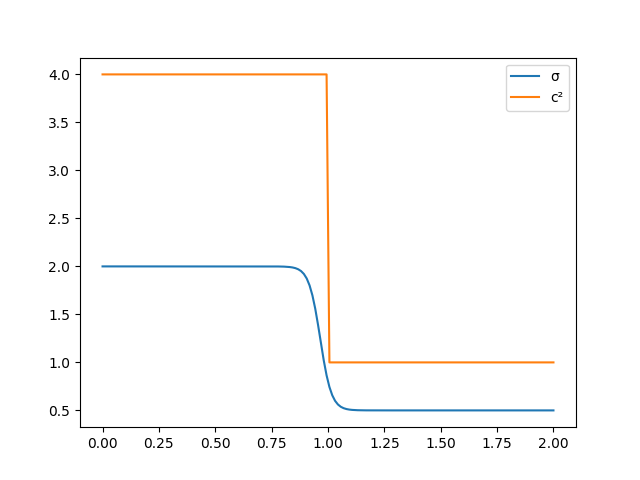
Example 2. We take the same , and but the different density and the squared speed of sound
with the smoothed jumps at . We set and , and the jump in is very steep, see Figure 1(a).
(a)
(b)
In this Example, for our values of and , but ; nevertheless, computations remain stable. Once again we choose the above versions and of the scheme parameters. The respective numerical results are shown in Tables 3 and 4. The original value is taken too rough, and the corresponding errors are large, but the further behaviour of the errors as grows is interesting and different from Example 1. For the next value , the practical convergence rates are higher than 2 though less than 3. But, for the further values and , is much higher than 4 and close to 6, and it becomes very close to 4 for the next . Concerning and , they are also higher than 4 for at least one of and .
We emphasize that for the error behaviour, the rate of smoothing of is definitive since is practically discontinuous for the chosen meshes. The phenomenon of the 4th order error behaviour for discontinuous is not elementary at all and needs more theoretical investigation since, in formulas (2.19) and (2.23) of the scheme, the second order difference operator is applied to the term including the multiplier .
The difference in the results between versions and is not so significant once again though the behaviour of , , and is generally more regular for the latter version.
| 10 | 20 | 4.171e-1 | 1.161 | 1.161 | ||||||
|---|---|---|---|---|---|---|---|---|---|---|
| 20 | 40 | 6.885e-2 | 6.058 | 2.599 | 2.236e-1 | 5.193 | 2.377 | 2.296e-1 | 5.058 | 2.339 |
| 40 | 80 | 1.149e-3 | 59.93 | 5.905 | 1.101e-2 | 20.31 | 4.344 | 1.784e-2 | 12.87 | 3.686 |
| 80 | 160 | 1.346e-5 | 85.37 | 6.416 | 5.355e-4 | 20.56 | 4.362 | 8.262e-4 | 21.59 | 4.433 |
| 160 | 320 | 8.356e-7 | 16.11 | 4.009 | 3.872e-5 | 13.83 | 3.790 | 3.872e-5 | 21.34 | 4.415 |
| 10 | 20 | 4.223e-1 | 1.151 | 1.151 | ||||||
|---|---|---|---|---|---|---|---|---|---|---|
| 20 | 40 | 6.858e-2 | 6.157 | 2.622 | 2.202e-1 | 5.229 | 2.387 | 2.202e-1 | 5.229 | 2.387 |
| 40 | 80 | 1.086e-3 | 63.17 | 5.981 | 7.712e-3 | 28.55 | 4.836 | 1.336e-2 | 16.47 | 4.042 |
| 80 | 160 | 1.984e-5 | 54.73 | 5.774 | 6.047e-4 | 12.75 | 3.673 | 6.554e-4 | 20.39 | 4.350 |
| 160 | 320 | 1.229e-6 | 16.15 | 4.013 | 4.544e-5 | 13.31 | 3.734 | 4.544e-5 | 14.42 | 3.850 |
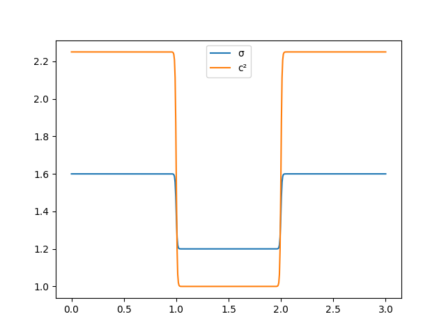
Example 3. In this example, we study the acoustic wave propagation in the three-layer-type medium in for and take the density and squared speed of sound in the form
with the smoothed jumps in the defining densities , 1.2 and 1.6 and speeds of sound , 1 and 1.5 in the left , middle and right layers in , respectively. We also set (physically, these parameters should be equal or close), so the jumps are steep, see Figure 1(b) where and are given for .
We also use the Ricker-type wavelet source function smoothed in space
with , where is the centre of . Note that then and for . The other data are zero: and .
For definiteness, we apply version A of the scheme parameters and choose and ; thus, and . For them, and ; the computations are stable again.
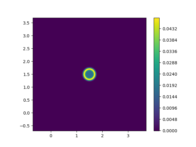
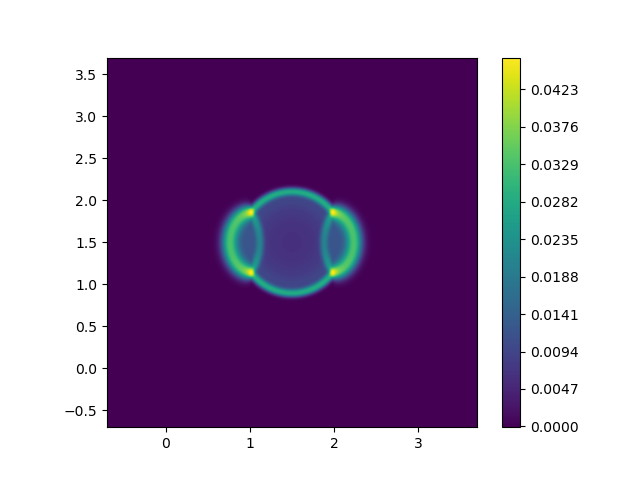
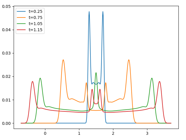
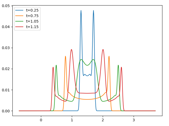
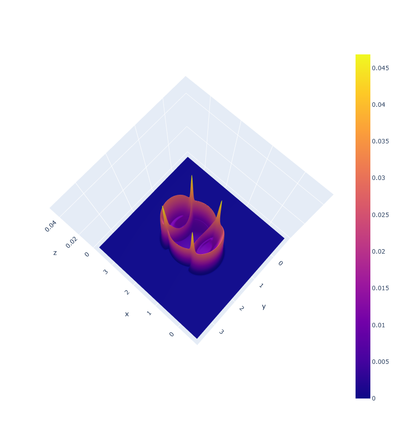
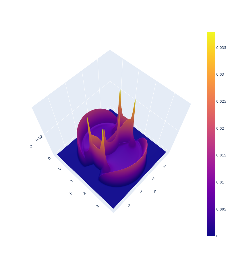
Contour levels of wavefields at six sequential characteristic time moments are presented in Fig. 2. The corresponding perpendicular central sections of the wavefields, for and , at four time moments are given in Fig. 3. We observe the wavefront generated by the source function expanding in the middle layer and then passing to the left and right layers with the higher speed of sound, together with the internal wavefronts reflected back from both the lines of jumps in and towards the centre of . The reflected waves meet at the centre and pass through each other. The results are given in the same manner and are close in general to those presented in [27], see also [13, 24], where similar but discontinuous and were taken. In addition, the 3D graphs of the wavefields at an intermediate and the final time moments are shown in Fig. 4. Such graphs are absent in [13, 24, 26], although they probably most evidently demonstrate the complex overall structure of the wavefields containing not only moving and reflected wavefronts but moving and incipient narrow peaks as well.
(a)
(b)
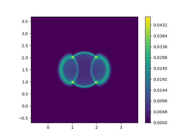
(c)
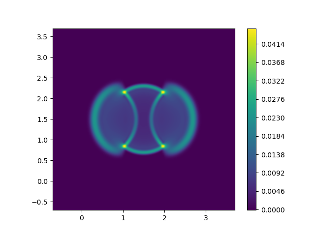
(d)
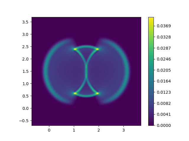
(e)

(f)
(a)
(b)
(a)
(b)
Acknowledgments
Support from the Basic Research Program at the HSE University (Laboratory of Mathematical Methods in Natural Science) is gratefully acknowledged by A. Zlotnik, Sections 1–2. Support from the Basic Research Program at the HSE University (International Centre of Decision Choice and Analysis) is gratefully acknowledged by T. Lomonosov, Section 3.
References
- [1] L.M. Brekhovskikh, O.A. Godin, Acoustics of Layered Media I. Plane and Quasi-plane Waves, Springer, Berlin, 2012. https://doi.org/10.1007/978-3-642-52369-4
- [2] S. Britt, E. Turkel, S. Tsynkov, A high order compact time/space finite difference scheme for the wave equation with variable speed of sound, J. Sci. Comput. 76(2) (2018) 777–811. https://doi.org/10.1007/s10915-017-0639-9
- [3] E. Burman, O. Duran, A. Ern, Hybrid high-order methods for the acoustic wave equation in the time domain, Commun. Appl. Math. Comput. 4(2) (2022) 597–633. https://doi.org10.1007/s42967-021-00131-8
- [4] L. Chen, J. Huang, L.-Y. Fu, W. Peng, C. Song, J. Han, A compact high-order finite-difference method with optimized coefficients for 2d acoustic wave equation, Remote Sens. 15 (2023) article 604. https://doi.org/ 10.3390/rs15030604
- [5] M. Ciment, S.H. Leventhal, Higher order compact implicit schemes for wave equation, Math. Comput. 29(132) (1975) 985–994.
- [6] B. Cockburn, Z. Fu, A. Hungria, L. Ji, M.A. Sánchez, F.-J. Sayas, Stormer-Numerov HDG methods for acoustic waves, J. Sci. Comput. 75 (2018) 597–624. https://doi.org/10.1007/s10915-017-0547-z
- [7] G.C. Cohen, Higher-Order Numerical Methods for Transient Wave Equations. Springer, Berlin, 2002. https://doi.org/10.1007/978-3-662-04823-8
- [8] G. Cohen, P. Joly, Construction and analysis of fourth-order finite difference schemes for the acoustic wave equation in non-homogeneous media, SIAM J. Numer. Anal. 4 (1996) 1266–1302. https://doi.org/10.1137/S0036142993246445
- [9] S. Das, W. Liao, A. Gupta, An efficient fourth-order low dispersive finite difference scheme for a 2-D acoustic wave equation, J. Comput. Appl. Math. 258 (2014) 151–167. http://dx.doi.org/10.1016/j.cam.2013.09.006
- [10] V.I. Fedorchuk, On the invariant solutions of some five-dimensional d’Alembert equations, J. Math. Sci. 220(1) (2017) 27–37. https://doi.org/10.1007/s10958-016-3165-7
- [11] Y. Jiang, Y. Ge, An explicit fourth-order compact difference scheme for solving the 2D wave equation, Adv. Difference Equat. 415 (2020) 1–14. https://doi.org/10.1186/s13662-020-02870-z
- [12] Y. Jiang, Y. Ge, An explicit high-order compact difference scheme for the three-dimensional acoustic wave equation with variable speed of sound, Int. J. Comput. Math. 100(2) (2023) 321–341. https://doi.org/10.1080/00207160.2022.2118524
- [13] B. Hou, D. Liang, H. Zhu, The conservative time high-order AVF compact finite difference schemes for two-dimensional variable coefficient acoustic wave equations, J. Sci. Comput. 80 (2019) 1279–1309. https://doi.org/10.1007/s10915-019-00983-6
- [14] D. Li, K. Li, W. Liao, A combined compact finite difference scheme for solving the acoustic wave equation in heterogeneous media, Numer. Meth. Partial Diff. Equat. 39 (2023) 4062–4086. https://doi.org/10.1002/num.23036
- [15] K. Li, W. Liao, Y. Lin, A compact high order alternating direction implicit method for three-dimensional acoustic wave equation with variable coefficient, J. Comput. Appl. Math. 361(1) (2019) 113–129. https://doi.org/10.1016/j.cam.2019.04.013
- [16] W. Liao, On the dispersion and accuracy of a compact higher-order difference scheme for 3D acoustic wave equation, J. Comput. Appl. Math. 270 (2014) 571–583. https://doi.org/10.1016/j.cam.2013.08.024
- [17] W. Liao, P. Yong, H. Dastour, J. Huang, Efficient and accurate numerical simulation of acoustic wave propagation in a 2D heterogeneous media, Appl. Math. Comput. 321 (2018) 385–400. https://doi.org/10.1016/j.amc.2017.10.052
- [18] A.A. Samarskii, Schemes of high-order accuracy for the multi-dimensional heat conduction equation, USSR Comput. Math. Math. Phys. 3(5) (1963) 1107–1146. https://doi.org/10.1016/0041-5553(63)90104-6
- [19] A.A. Samarski, V.B. Andréiev, Métodos en Diferencias para las Ecuaciones Elípticas, Mir, Moscú, 1979.
- [20] S. Schoeder, M. Kronbichler, W.A. Wall, Arbitrary high-order explicit hybridizable discontinuous Galerkin methods for the acoustic wave equation, J. Sci. Comput. 76 (2018) 969–1006. https://doi.org/10.1007/s10915-018-0649-2
- [21] F. Smith, S. Tsynkov, E. Turkel, Compact high order accurate schemes for the three dimensional wave equation, J. Sci. Comput. 81(3) (2019) 1181–1209. https://doi.org/10.1007/s10915-019-00970-x
- [22] A. Zlotnik, On properties of an explicit in time fourth-order vector compact scheme for the multidimensional wave equation, Preprint (2021) 1–15. https://arxiv.org/abs/2105.07206
- [23] A. Zlotnik, R. Čiegis, On higher-order compact ADI schemes for the variable coefficient wave equation, Appl. Math. Comput. 412 (2022) article 126565. https://doi.org/10.1016/j.amc.2021.126565
- [24] A. Zlotnik, R. Čiegis, On construction and properties of compact 4th order finite-difference schemes for the variable coefficient wave equation, J. Sci. Comput. 95(1) (2023) article 3. https://doi.org/10.1007/s10915-023-02127-3
- [25] A. Zlotnik, O. Kireeva, On compact 4th order finite-difference schemes for the wave equation, Math. Model. Anal. 26(3) (2021) 479–502. https://doi.org/10.3846/mma.2021.13770
- [26] A. Zlotnik, T. Lomonosov, On stability and error bounds of an explicit in time higher-order vector compact scheme for the multidimensional wave and acoustic wave equations, Appl. Numer. Math. 195 (2024) 54–74. https://doi.org/10.1016/j.apnum.2023.09.006
- [27] A. Zlotnik, T. Lomonosov, On a semi-explicit fourth-order vector compact scheme for the acoustic wave equation, Russ. J. Numer. Anal. Math. Model. 40 (1) (2025) 71–88. https://doi.org/10.1515/rnam-2025-0006