Error Optimization: Overcoming Exponential Signal Decay in Deep Predictive Coding Networks

Abstract

Predictive Coding (PC) offers a biologically plausible alternative to backpropagation for neural network training, yet struggles with deeper architectures. This paper identifies the root cause: an inherent signal decay problem where gradients attenuate exponentially with depth, becoming computationally negligible due to numerical precision constraints. To address this fundamental limitation, we introduce Error Optimization (EO), a novel reparameterization that preserves PC’s theoretical properties while eliminating signal decay. By optimizing over prediction errors rather than states, EO enables signals to reach all layers simultaneously and without attenuation, converging orders of magnitude faster than standard PC. Experiments across multiple architectures and datasets demonstrate that EO matches backpropagation’s performance even for deeper models where conventional PC struggles. Besides practical improvements, our work provides theoretical insight into PC dynamics and establishes a foundation for scaling biologically-inspired learning to deeper architectures on digital hardware and beyond.

State Optimization (standard)

Error Optimization (ours)

Figure 1: Evolution of layerwise energies during optimization. Standard PC’s State Optimization struggles to propagate signals through the network, with progressively longer delays at deeper layers.By contrast, our Error Optimization enables global signal propagation and converges to equilibrium in just a fraction of the time. Results for an untrained 20-layer MLP on a random MNIST input.

1 Introduction

Neural networks have revolutionized machine learning, yet their learning algorithms often diverge from biological reality [46, 32]. Predictive Coding (PC) stands as a prominent neuroscience theory aiming to explain how the brain processes sensory information through hierarchical prediction and error propagation [34, 50]. In recent years, researchers have reformulated PC as a general machine learning algorithm, offering a biologically plausible alternative to backpropagation for training neural networks [41, 43, 46, 52].

Its theoretical appeal is significant: through purely local learning rules, PC is able to approximate backpropagation, with mathematical equivalence established under specific conditions [48, 51]. However, despite this promising connection, PC has struggled to scale beyond simple problems and baseline architectures [52]. A particularly concerning observation is that deeper PC models often perform worse than shallower ones [62], contrary to the pattern seen with backpropagation, where depth typically improves representational capacity.

Computational demands further complicate PC’s scaling challenges. During training, PC requires an internal energy minimization process that converges to equilibrium states through iterative updates. While ideally suited for neuromorphic hardware with parallel, local updates, PC research has predominantly relied on conventional GPU implementations, with a significant computational overhead compared to backpropagation’s direct gradient calculation. This hardware-algorithm mismatch presents a practical barrier to widespread adoption, hindering progress in the field.

The PC community has pursued several approaches to address these computational inefficiencies. Some have focused on improving the optimization process itself through different optimizers and JIT-compiled implementations [62, 57]. Others have explored fast approximate one-step regimes [59], modified update orders from parallel to sequential [56], or amortized inference to estimate the equilibrium states using auxiliary networks [54]. Despite these advances, substantial gaps remain in both computational efficiency and theoretical understanding of PC.

In this paper, we address the fundamental limitations of PC’s digital simulation–which currently represents nearly all practical PC research. Our work connects the seemingly disparate problems of depth scaling and computational efficiency in PC networks, uncovering a common underlying cause and providing an elegant solution.

Our contributions

• We identify a fundamental mechanism of exponential signal decay in traditional PC, whereby signals attenuate as they propagate through the network. This previously undetected issue explains why deeper PC networks underperform and require excessive computation.

• We introduce Error Optimization (EO), a novel reparameterization of PC that preserves theoretical equivalence while resolving the signal decay problem. By optimizing over prediction errors rather than neural states, EO restructures the computational graph from locally to globally connected, enabling signals to propagate unattenuated to all layers simultaneously, while preserving PC’s defining property of local weight updates.

• We empirically demonstrate that EO converges orders of magnitude faster than traditional PC on deep networks, resolving a major computational bottleneck in PC research.

• Through comprehensive experiments across architectures of varying depths, we demonstrate that EO consistently achieves performance comparable to backpropagation, providing a definitive solution to PC’s depth scaling issues.

• With computational limitations addressed through EO, we argue for a shift in PC research, focussing on long-term impact beyond proof-of-concepts. We point out two promising research directions enabled by EO, each from a different hardware perspective.

2 Predictive Coding as an Optimization over States

((a)) State Optimization, the standard formulation of PC with a locally connected computational graph

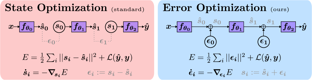
((b)) Error Optimization, our reparametrization of PC with a fully connected (global) graph structure

Figure 2: Structural comparison of SO (left) and EO (right), highlighting functional equivalence

To establish the groundwork for our contributions, we first present the conventional formulation of PC as an optimization over neural states. We will refer to this as State Optimization (SO).

In SO (and PC in general), each layer attempts to predict the state of the next layer. The main goal is to minimize $E$, the sum of all prediction errors, typically expressed as an energy function:

$$E(\bm{s},\bm{\theta})=\frac{1}{2}\sum_{i=0}^{L}\|\bm{s_{i}}-\bm{\hat{s}_{i}}\|^{2},$$ (1)

where $\bm{s_{i}}$ denotes the neural state at layer $i$ and $\bm{\hat{s}_{i}}:=\bm{f_{\theta_{i}}}(\bm{s_{i-1}})$ the parametrized prediction of $\bm{s_{i}}$ based on the preceding layer’s state $\bm{s_{i-1}}$. Fig.˜2(a) illustrates this graphically. For ease of notation, we define $\bm{s_{-1}}:=\bm{x}$ and $\bm{s_{L}}:=\bm{y}$, representing input data and target output, respectively.

Implicitly, Eq.˜1 corresponds to a squared error loss on the predicted output $\hat{\bm{y}}:=\bm{\hat{s}_{L}}$. Alternative losses, such as cross-entropy, are also allowed [53], reformulating the PC energy function to its more general form with a generic output loss $\mathcal{L}$:

$$E(\bm{s},\bm{\theta})=\frac{1}{2}\sum_{i=0}^{L-1}\|\bm{s_{i}}-\bm{\hat{s}_{i}}\|^{2}+\mathcal{L}(\hat{\bm{y}},\bm{y}).$$ (2)

A single training step in SO consists of a two-phased energy minimization of $E(\bm{s},\bm{\theta})$:

1. State updates: With $\bm{\theta}$ kept fixed, the states $\bm{s}$ are iteratively updated to minimize $E$ via gradient descent, until equilibrium is reached. The state dynamics for layer $i$ follow:

   $$\hskip-28.0pt{\color[rgb]{.5,.5,.5}\dot{\bm{s}}_{\!\bm{i}}:=}\>\frac{\partial\bm{s_{i}}}{\partial t}=-\bm{\nabla}_{\bm{s_{i}}}E(\bm{s},\bm{\theta})=-\bm{\epsilon_{i}}+\bm{\epsilon_{i+1}}\ \frac{\partial\bm{f_{\theta_{i+1}}}}{\partial\bm{s_{i}}}(\bm{s_{i}}),$$

   where $\bm{\epsilon_{i}}:=\bm{s_{i}}-\bm{\hat{s}_{i}}$ represents the layerwise prediction error.

2. Weight update: With $\bm{s}$ kept fixed, the parameters $\bm{\theta}$ are updated once, further minimizing $E$:

   $$\hskip-42.0pt\Delta\bm{\theta_{i}}\propto-\bm{\nabla}_{\bm{\theta_{i}}}E(\bm{s},\bm{\theta})=\bm{\epsilon_{i}}\ \frac{\partial\bm{f_{\theta_{i}}}}{\partial\bm{\theta_{i}}}(\bm{s_{i-1}})$$

Full training involves repeating this procedure over numerous data batches, as in standard Deep Learning. The distinctive feature of PC, however, is that both phases can be implemented efficiently in biological neural circuits with strictly local computation [43, 46].

Feedforward state initialization

It is common practice to set the initial states $\bm{s}^{t=0}$ via a feedforward pass of the input $\bm{x}$ through the network. At each layer, the prediction $\bm{\hat{s}_{i}}$ is copied onto $\bm{s_{i}}$, initializing the local prediction error $\bm{\epsilon_{i}}$ to exactly zero. Despite lacking theoretical justification, the technique is widely used due to its empirical success in accelerating the state optimization process.

3 The Problem of Exponential Signal Decay in State Optimization

In this section, we uncover a previously unidentified phenomenon in PC networks: the exponential decay of signal propagation throughout SO. This discovery represents a fundamental limitation that affects the scalability of deep PC networks and helps explain the performance gap with backpropagation, which was observed to worsen for deeper models [62].

3.1 Theoretical Expectation vs. Empirical Reality

In SO, after feedforward state initialization, all energies are zero except for the output loss $\mathcal{L}$. Next, during state updates, we expect a backward signal to travel continuously from output to input, advancing one layer per update step. The theory suggests a clear chain reaction: non-zero energy at any layer should induce changes in neighboring states, thereby continuously propagating the signal further down the network.

However, our empirical observations contradict this expectation. Fig.˜1 illustrates how, in practice, the signal travels discontinuously through the network, halting at deeper layers with progressively longer delays. Paradoxically, we observe that a non-zero energy at one layer fails to immediately propagate to adjacent layers, remaining dormant for multiple update steps before inducing detectable changes. Moreover, this behavior seems to scale logarithmically with time, suggesting that exponentially many update steps would be required for signals to reach the bottom layers—an impractical computational requirement.

3.2 Mechanism of Signal Decay

Backward wavefront dynamics

The state update dynamics at the start of optimization provide insight into the cause of this suppressed signal propagation. Below, in Fig.˜3, we present a step-by-step description of the initial wavefront travelling backwards through the network.

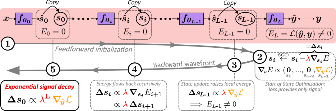
To reduce clutter, layer effects are folded into the $\propto$-sign, which indicates matrix proportionality.

Figure 3: Step-by-step dynamics of SO reveals an exponential signal decay in the backward path.

Our analysis uncovers a signal decay mechanism: when an energy gradient propagates from one layer to the next, it is attenuated by the state learning rate $\lambda$ (necessarily < 1 for stability). With each subsequent layer traversal, this attenuation compounds multiplicatively, resulting in exponential decay with respect to network depth.

Appendix˜B extends this analysis beyond the wavefront, deriving a mathematical characterization of early state dynamics across the entire network, with a connection to Pascal’s triangle.

Numerical precision constraints

In theory, signals should still advance consistently at each update step, regardless of how small they become. However, in practice, digital implementations face a fundamental constraint: limited numerical precision. Specifically, the concept of “machine epsilon” becomes relevant: the smallest value that, when added to $1.0$, yields a result distinguishable from $1.0$. With standard 32-bit floating-point arithmetic, additions involving numbers that differ by approximately eight orders of magnitude (e.g., $10^{-8}$ and $1.0$) result in the smaller number being effectively truncated to zero.

With typical state learning rates of the order of $10^{-2}$ to $10^{-1}$, signals attenuate below this threshold within just 4 to 8 update steps. This explains why theoretically continuous propagation manifests as discrete, delayed jumps in practice, with increasingly pronounced effects at greater network depths.

3.3 Implications for Deep PC Networks

This exponential signal decay has profound implications for the digital simulation of PC networks. First and foremost, deeper layers may remain entirely untrained if optimization terminates before signals reach them, such that they effectively represent purely random input transformations. Such incomplete training would be hard to detect from state convergence metrics alone, which may incorrectly suggest equilibrium has been reached when in reality, these layers have yet to begin meaningful optimization.

A more nuanced implication emerges when considering which signals do successfully penetrate the network. Only hard-to-classify or mislabeled inputs could produce output gradients $\bm{\nabla_{\!\hat{y}}}\mathcal{L}$ that are large enough to overcome the exponential attenuation, potentially creating a systemic bias where different layers of the feedforward network train on different subsets of the data distribution.

Even when signals eventually reach deeper layers, the ensuing state modification will struggle to propagate back to upper layers. This creates a persistent misalignment where top layers, despite receiving strong output signals, cannot efficiently adapt to changes in deeper representations. While feedforward state initialization partially mitigates this issue, it cannot eliminate the intrinsic interdependencies that exist between states throughout optimization.

We argue that this signal propagation challenge represents a significant theoretical and practical limitation to scaling PC networks to greater depths. Standard remedies, like increased learning rates, higher numerical precision, or alternative optimizers, address symptoms without resolving the core issue, highlighting the need for a fundamental reconsideration of PC optimization strategies.

4 From States to Errors: Reparametrizing for Improved Signal Propagation

We introduce Error Optimization (EO), a novel reparameterization of Predictive Coding that directly addresses the exponential signal decay problem identified in the previous section.

The key insight of EO is to reformulate PC dynamics in terms of errors rather than states. By restructuring the computational graph from locally to globally connected, EO enables signals to reach all layers simultaneously without attenuation, while preserving the local weight update property that distinguishes PC from standard backpropagation.

4.1 Mathematical Formulation

EO reparameterizes PC by making the layerwise prediction errors $\bm{\epsilon}$ the primary variables to optimize, rather than the states $\bm{s}$. The energy function remains the same, now formulated as:

$$E(\bm{\epsilon},\bm{\theta})=\frac{1}{2}\sum_{i=0}^{L}\|\bm{\epsilon_{i}}\|^{2}+\mathcal{L}(\hat{\bm{y}},\bm{y}).$$ (3)

Optionally, states can be derived from errors through the recursive relationship $\bm{s_{i}}:=\bm{\hat{s}_{i}}+\bm{\epsilon_{i}}$, where still $\bm{\hat{s}_{i}}:=\bm{f_{\theta_{i}}}(\bm{s_{i-1}})$. Conceptually, this amounts to a feedforward pass starting from input $\bm{x}$ with perturbations $\bm{\epsilon_{i}}$ applied at each layer. This is graphically shown in Fig.˜2(b).

The core dynamics remain unchanged: during training, errors $\bm{\epsilon}$ are iteratively updated to minimize $E$, followed by a gradient step to further minimize $E$ with respect to $\bm{\theta}$. Crucially, EO maintains the local nature of weight updates, preserving a fundamental principle of PC. Fig.˜4 demonstrates the close algorithmic parallels between SO and EO, with a more extended comparison given in Fig.˜A.1.

For a formal proof of theoretical equivalence between SO and EO, we refer readers to Section˜C.1.

4.2 Computational Advantages: Resolving the Signal Decay Problem

The key difference between SO and EO lies in their computational graph structures, as shown in Fig.˜2. While SO intentionally breaks the computational graph to enforce local update information, EO reconnects the entire network graph, thereby creating a direct relationship between all input variables and the predicted output:

$$\textbf{(EO)}\quad\hat{\bm{y}} =\text{func}(\bm{x},\bm{\epsilon_{0}},\bm{\epsilon_{1}},\dots,\bm{\epsilon_{L-1}})$$

$$\text{vs. }\textbf{(SO)}\quad\hat{\bm{y}} =\text{func}(\bm{s_{L-1}})$$

This restructuring enables the main advantage of EO: the use of backpropagation to transmit signals from the output loss $\mathcal{L}(\hat{\bm{y}},\bm{y})$ directly to all errors $\bm{\epsilon_{i}}$ via $\hat{\bm{y}}$, without intermediate attenuation.

A brief step-by-step analysis reveals how EO successfully decouples stability from propagation speed, which were problematically intertwined in SO. First, backpropagation computes gradients throughout the entire network, ensuring signals reach all layers unattenuated. Only thereafter, during the actual error update step, is the learning rate applied, affecting stability but not propagation reach. This separation allows signals to influence all network layers simultaneously, regardless of depth, thereby eliminating the exponential decay problem seen in SO.

Algorithm 1 ​:  State Optimization (standard)

1:State updates

2:Initialize states $\{\bm{s_{i}}\}\leftarrow\texttt{ff\_init}(\bm{x})$

3:for $t=1$ to $T$ do

4:  $\bm{s_{-1}}\leftarrow\bm{x}$

5:  for $i=0$ to $L-1$ do $\triangleright$ Parallel

6:   $\bm{\hat{s}_{i}}\leftarrow\bm{f_{\theta_{i}}}(\bm{s_{i-1}})$

7:   $\bm{\epsilon_{i}}\leftarrow\bm{s_{i}}-\bm{\hat{s}_{i}}$   

8:  $\hat{\bm{y}}\leftarrow\bm{f_{\theta_{L}}}(\bm{s_{L-1}})$

9:  $E\leftarrow\frac{1}{2}\sum_{i=0}^{L-1}\|\bm{s_{i}}-\bm{\hat{s}_{i}}\|^{2}+\mathcal{L}(\hat{\bm{y}},\bm{y})$

10:  $\bm{\nabla}_{\!{\color[rgb]{0.83984375,0.15234375,0.15625}\bm{s_{j}}}}E\leftarrow\color[rgb]{0.83984375,0.15234375,0.15625}\bm{\epsilon_{j}}-\frac{\partial\bm{\hat{s}_{j+1}}}{\partial\bm{s_{j}}}^{T}\bm{\epsilon_{j+1}}$ $\triangleright$ Local

11:  ${\color[rgb]{0.83984375,0.15234375,0.15625}\bm{s_{j}}}\leftarrow{\color[rgb]{0.83984375,0.15234375,0.15625}\bm{s_{j}}}-\lambda\bm{\nabla}_{\!{\color[rgb]{0.83984375,0.15234375,0.15625}\bm{s_{j}}}}E$ for all $j$

12:Weight update

13:$\bm{\nabla}_{\!\bm{\theta_{j}}}E\leftarrow-\frac{\partial\bm{\hat{s}_{j}}}{\partial\bm{\theta_{j}}}^{T}\bm{\epsilon_{j}}$ $\triangleright$ Local

14:$\bm{\theta_{j}}\leftarrow\bm{\theta_{j}}-\eta\bm{\nabla}_{\bm{\theta_{j}}}E$ for all $j$

Algorithm 2 ​:  Error Optimization (ours)

1:Error updates

2:Initialize errors $\{\bm{\epsilon_{i}}\}\leftarrow\texttt{zero\_init}$

3:for $t=1$ to $T$ do

4:  $\bm{s_{-1}}\leftarrow\bm{x}$

5:  for $i=0$ to $L-1$ do $\triangleright$ Sequential

6:   $\bm{\hat{s}_{i}}\leftarrow\bm{f_{\theta_{i}}}(\bm{s_{i-1}})$

7:   $\bm{s_{i}}\leftarrow\bm{\hat{s}_{i}}+\bm{\epsilon_{i}}$   

8:  $\hat{\bm{y}}\leftarrow\bm{f_{\theta_{L}}}(\bm{s_{L-1}})$

9:  $E\leftarrow\frac{1}{2}\sum_{i=0}^{L-1}\|\bm{\epsilon_{i}}\|^{2}+\mathcal{L}(\hat{\bm{y}},\bm{y})$

10:  $\bm{\nabla}_{\!{\color[rgb]{0,0,1}\bm{\epsilon_{j}}}}E\leftarrow\color[rgb]{0,0,1}\bm{\epsilon_{j}}+\frac{\partial\hat{\bm{y}}}{\partial\bm{\epsilon_{j}}}^{T}\bm{\nabla}_{\!\hat{\bm{y}}}\mathcal{L}$ $\triangleright$ Backprop

11:  ${\color[rgb]{0,0,1}\bm{\epsilon_{j}}}\leftarrow{\color[rgb]{0,0,1}\bm{\epsilon_{j}}}-\lambda\bm{\nabla}_{\!{\color[rgb]{0,0,1}\bm{\epsilon_{j}}}}E$ for all $j$

12:Weight update

13:$\bm{\nabla}_{\!\bm{\theta_{j}}}E\leftarrow-\frac{\partial\bm{\hat{s}_{j}}}{\partial\bm{\theta_{j}}}^{T}\bm{\epsilon_{j}}$ $\triangleright$ Local

14:$\bm{\theta_{j}}\leftarrow\bm{\theta_{j}}-\eta\bm{\nabla}_{\bm{\theta_{j}}}E$ for all $j$

Figure 4: Algorithmic comparison of SO vs. EO, with structural differences highlighted in color. Loops over $j$ are omitted for brevity. An extended version is provided in Appendix˜A.

4.3 Proof-of-Concept on MNIST

To evaluate the practical advantages of EO over SO, we compared the two methods for a 20-layer linear PC network trained on MNIST. This architecture provides an ideal testbed as it offers a unique and analytically tractable equilibrium state. For an unbiased comparison, we used identical network weights for both approaches (obtained through backpropagation as neutral method), with hyperparameters optimized for convergence speed. Complete details are provided in Section˜C.3.

Fig.˜5 illustrates how both SO and EO converge to the analytical optimum, confirming their theoretical equivalence. However, for the exact same model, EO converges roughly $100\times$ faster than SO, a dramatic difference in speed that highlights EO’s practical advantage for training deep PC networks.

The figure also provides further evidence for the discontinuous signal propagation issue identified in Section˜3. In SO, the signal takes roughly 30 steps to advance 9 layers and reach $\bm{s_{9}}$, and nearly 100 steps to traverse the 20-layer network and reach $\bm{s_{0}}$. By contrast, EO’s global connectivity enables immediate signal propagation across the network, allowing all layers to optimize simultaneously.

Additional experiments with deep non-linear MLPs (see Section˜C.4) yielded similar results, with EO consistently outperforming SO in terms of convergence speed. Notably, SO required an impractical number of update steps (>100,000) to reach convergence, reinforcing the necessity of our EO reformulation for scaling PC to deeper networks.

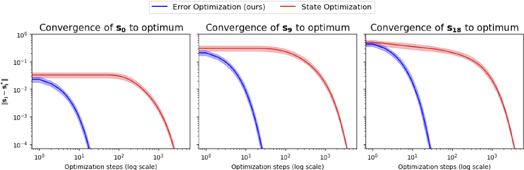
Figure 5: State convergence dynamics of bottom, middle, and top hidden layers in a 20-layer linear PC network trained on MNIST. Curves show batch medians (n=64) of L2 deviation from the analytical equilibrium, with interquartile shading. Error Optimization converges over $100\times$ faster than State Optimization for the same model.

4.4 Implications for Deep PC Networks

The benefits of EO’s improved signal propagation extend beyond faster convergence, addressing several fundamental limitations of SO. Most importantly, by providing signal to all layers from the first step, EO completely resolves the issue of untrained deep layers. It enables all layers to begin optimization simultaneously, regardless of network depth.

Furthermore, EO eliminates the potential systemic bias in SO, where only inputs generating large output gradients could successfully influence deeper layers. With EO, all inputs contribute equally to training at all depths, promoting uniform learning across the network.

Moreover, any change in deeper layers is efficiently communicated to the upper layers through the feedforward pass required for $\hat{\bm{y}}$. This bidirectional efficiency explains why the widely-used feedforward state initialization heuristic in PC works so well: it essentially implements the first step of EO. Our formulation thus provides theoretical backing for this empirical practice while extending its benefits throughout the optimization process.

By resolving these fundamental limitations, EO establishes a solid foundation for scaling PC to deeper architectures. Our MNIST proof-of-concept demonstrates significant convergence improvements, validating this theoretical advancement and motivating large-scale empirical evaluation.

5 Experiments

To evaluate EO’s effectiveness in training deep networks, we conducted extensive experiments comparing EO against both SO and backpropagation. Our experimental design follows the benchmark established by [62], allowing direct comparison with their findings.

5.1 Experimental Setup

We evaluated performance across four standard computer vision datasets: MNIST [33, 42], FashionMNIST [44], and CIFAR-10/100 [35].The architecture selection spanned an MLP, VGG-style convolutional networks of various depths [38], and a deep residual network [39].

Complete implementation details, including hyperparameter settings, are provided in Appendix˜D.

All code is available at https://github.com/cgoemaere/pc_error_optimization.

5.2 Results and Analysis

Table 1: Test accuracies (in %) of EO, SO and backprop for various models, losses, and datasets. Bold indicates best results within confidence intervals (mean ± 1 std. dev.; taken over 5 seeds).

Loss $\mathcal{L}$	Mean Squared Error			Cross-Entropy
Training algorithm	EO	SO	Backprop	EO	SO	Backprop
MLP (4 layers)
MNIST	$\mathbf{98.28^{\pm 0.09}}$	$\mathbf{98.42^{\pm 0.08}}$	$\mathbf{98.30^{\pm 0.15}}$	$\mathbf{98.11^{\pm 0.08}}$	$\mathbf{98.01^{\pm 0.15}}$	$\mathbf{98.13^{\pm 0.08}}$
FashionMNIST	$87.02^{\pm 0.24}$	$88.01^{\pm 0.09}$	$\mathbf{88.79^{\pm 0.21}}$	$87.58^{\pm 0.13}$	$88.00^{\pm 0.24}$	$\mathbf{88.87^{\pm 0.27}}$
VGG-5
CIFAR-10	$\mathbf{88.70^{\pm 0.12}}$	$86.67^{\pm 0.20}$	$\mathbf{88.58^{\pm 0.12}}$	$\mathbf{88.27^{\pm 0.18}}$	$84.66^{\pm 0.33}$	$\mathbf{87.95^{\pm 0.29}}$
CIFAR-100 (Top-1)	$64.37^{\pm 0.17}$	$50.41^{\pm 1.45}$	$\mathbf{64.80^{\pm 0.24}}$	$63.39^{\pm 0.25}$	$56.85^{\pm 0.69}$	$\mathbf{63.83^{\pm 0.15}}$
CIFAR-100 (Top-5)	$85.28^{\pm 0.38}$	$77.41^{\pm 1.21}$	$85.80^{\pm 0.13}$	$\mathbf{87.34^{\pm 0.14}}$	$83.11^{\pm 0.19}$	$\mathbf{87.43^{\pm 0.06}}$
VGG-7
CIFAR-10	$\mathbf{88.98^{\pm 0.19}}$	$77.79^{\pm 0.34}$	$\mathbf{88.94^{\pm 0.32}}$	$88.84^{\pm 0.31}$	$77.98^{\pm 0.40}$	$\mathbf{89.60^{\pm 0.16}}$
CIFAR-100 (Top-1)	$\mathbf{66.55^{\pm 0.45}}$	$42.90^{\pm 0.43}$	$\mathbf{66.23^{\pm 0.42}}$	$58.62^{\pm 0.20}$	$53.45^{\pm 0.38}$	$\mathbf{65.14^{\pm 0.29}}$
CIFAR-100 (Top-5)	$\mathbf{85.65^{\pm 0.12}}$	$70.01^{\pm 0.52}$	$84.10^{\pm 0.39}$	$85.09^{\pm 0.14}$	$80.48^{\pm 0.38}$	$\mathbf{88.60^{\pm 0.24}}$
VGG-9
CIFAR-10	$88.80^{\pm 0.71}$	$76.40^{\pm 0.20}$	$\mathbf{90.04^{\pm 0.50}}$	$86.81^{\pm 0.09}$	$78.60^{\pm 0.30}$	$\mathbf{89.76^{\pm 0.20}}$
CIFAR-100 (Top-1)	$61.35^{\pm 0.76}$	$45.70^{\pm 0.14}$	$\mathbf{66.28^{\pm 0.29}}$	$\mathbf{60.65^{\pm 0.25}}$	$54.19^{\pm 0.41}$	$\mathbf{61.11^{\pm 0.45}}$
CIFAR-100 (Top-5)	$\mathbf{84.74^{\pm 0.40}}$	$73.04^{\pm 0.46}$	$\mathbf{84.96^{\pm 0.29}}$	$\mathbf{85.84^{\pm 0.15}}$	$80.65^{\pm 0.41}$	$85.14^{\pm 0.32}$
ResNet-18
CIFAR-10	$\mathbf{92.17^{\pm 0.26}}$	“$53.74^{\pm 0.43}$”	$\mathbf{92.36^{\pm 0.12}}$	$\mathbf{91.73^{\pm 0.21}}$	“$43.19^{\pm 0.61}$”	$\mathbf{91.85^{\pm 0.24}}$
CIFAR-100 (Top-1)	$68.52^{\pm 0.34}$	“$22.83^{\pm 0.38}$”	$\mathbf{69.94^{\pm 0.54}}$	$69.47^{\pm 0.32}$	“$16.01^{\pm 0.42}$”	$\mathbf{71.46^{\pm 0.32}}$
CIFAR-100 (Top-5)	$86.86^{\pm 0.44}$	“$50.18^{\pm 0.52}$”	$\mathbf{87.76^{\pm 0.41}}$	$90.47^{\pm 0.12}$	“$40.67^{\pm 0.70}$”	$\mathbf{91.91^{\pm 0.23}}$
“…”: ResNet-18 was unstable in our SO experiments, so we copied the results from [62]

Our results confirm the significant performance gap between SO and backpropagation previously reported by [62], while demonstrating that EO substantially narrows this gap.

Several key findings emerge from our experiments:

• Depth scaling: EO exhibits the expected performance improvement with increasing network depth, similar to backpropagation, whereas SO performance degraded in deeper networks. This is most noticeable for ResNet-18, where EO achieved competitive performance while SO suffered from instability issues in our implementation.

• Performance parity: EO nearly matches backpropagation’s performance across most datasets and architectures, with results falling within statistical confidence intervals in many cases.

• Loss function effects: Both Mean Squared Error (MSE) and Cross-Entropy (CE) loss functions resulted in comparable performance across experimental settings, despite CE’s typically superior gradient properties compared to MSE. However, we did observe greater sensitivity to hyperparameter selection with CE loss in both EO and SO algorithms.

Overall, our experimental results validate EO’s theoretical advantages. By resolving SO’s signal decay problem, EO successfully scales PC to deeper architectures, unlocking its ability to handle substantially more complex machine learning challenges than previously possible.

6 Conclusion and Future Directions

This paper identifies and addresses a fundamental limitation in Predictive Coding networks: the exponential decay of signal propagation during State Optimization. Our proposed Error Optimization overcomes this limitation by restructuring PC’s computational graph while preserving theoretical equivalence, achieving dramatic performance improvements without sacrificing the local weight update property that distinguishes PC from backpropagation.

6.1 Reinterpreting Predictive Coding

EO provides a fresh perspective on PC’s energy minimization process. Essentially, PC searches for minimal-norm layerwise perturbations that collectively produce optimal outputs. At each layer, these corrections are added to the feedforward pass, incrementally refining the final output prediction. From these targeted state modifications, local weight learning rules can then be derived.

Further insights can be gained from the perspective of PC as a variational Bayes algorithm [41, 34, 50] for full-distribution generative modelling [58, 61]. Here, EO functionally mirrors the highly successful VAE reparameterization trick [36], thereby providing a principled basis for scaling PC to large generative architectures, including language models [53].

6.2 Predictive Coding Beyond The Hardware Lottery

Algorithmic success is often dictated not by theoretical merit but by compatibility with prevailing hardware [49]. Serving as a prime example, PC has struggled to prove its worth despite theoretical soundness. To unlock its full potential, EO reformulates PC in a way that aligns naturally with digital processors, supporting efficient backpropagation and fast convergence across deep networks. Meanwhile, SO remains highly relevant for neuromorphic implementations, where physical energy minimization would occur naturally and near-instantaneously, regardless of network depth.

Despite their structural differences, both approaches still minimize the same energy function to reach identical equilibria. This functional equivalence creates a pragmatic research methodology: rather than being limited by SO’s digital inefficiency, researchers can turn to EO for rapid prototyping, generating insights that remain valid for understanding biologically-plausible PC mechanisms.

6.3 The Road Ahead for Predictive Coding

With PC’s viability as a learning algorithm now firmly established, research must shift from proof-of-concept to practical impact. We highlight two research directions with great potential:

1. Unblocking neuromorphic hardware development: Despite its theoretical suitability for ultra-energy-efficient neuromorphic implementation, hardware development for PC has been scarce. A key obstacle is our limited understanding of PC’s behavior at exact equilibrium—the regime to which any physical implementation would naturally settle. Yet, our experiments consistently preferred hyperparameter configurations of approximate backpropagation, leaving little appeal to hardware developers. With EO as an efficient tool to study equilibrium dynamics, research can finally begin to address this critical barrier to neuromorphic advancement.

2. Identifying PC’s distinctive advantages: Rather than competing with backpropagation in its domains of strength, research should focus on areas where PC uniquely excels. As [60] demonstrated with online and continual learning, such domains exist but remain underexplored. Although EO’s reliance on backpropagation puts an upper limit on PC’s computational efficiency [55, as noted before in], few-step EO could offer a compromise that maintains PC’s unique properties while keeping training times practical.

With EO effectively addressing PC’s computational limitations on digital hardware, the field must now face its true test: demonstrating that Predictive Coding offers substantive advantages in specific domains, sufficient to justify its adoption over established approaches.

[sorting=nyt]

Appendix A Full comparison: State Optimization vs. Error Optimization

Algorithm 3 ​:  State Optimization (standard)

1:Input $\bm{x}$, target $\bm{y}$, layers $\{\bm{f_{\theta_{i}}}\}_{i=0}^{L}$,

2:optimization steps $T$, state learning rate $\lambda$,

3:weight learning rate $\eta$, output loss $\mathcal{L}$

4:

5:Feedforward state initialization (ff_init)

6:$\bm{s_{-1}}\leftarrow\bm{x}$

7:for $i=0$ to $L-1$ do $\triangleright$ Sequential

8:  $\bm{\hat{s}_{i}}\leftarrow\bm{f_{\theta_{i}}}(\bm{s_{i-1}})$

9:  $\bm{s_{i}}\leftarrow\bm{\hat{s}_{i}}$

10:

11:State updates

12:for $t=1$ to $T$ do

13:

14:  for $i=0$ to $L-1$ do $\triangleright$ Parallel

15:   $\bm{\hat{s}_{i}}\leftarrow\bm{f_{\theta_{i}}}(\bm{s_{i-1}})$

16:   $\bm{\epsilon_{i}}\leftarrow\bm{s_{i}}-\bm{\hat{s}_{i}}$   

17:  $\hat{\bm{y}}\leftarrow\bm{f_{\theta_{L}}}(\bm{s_{L-1}})$

18:  $E\leftarrow\frac{1}{2}\sum_{i=0}^{L-1}\|\bm{s_{i}}-\bm{\hat{s}_{i}}\|^{2}+\mathcal{L}(\hat{\bm{y}},\bm{y})$

19:   Local energy gradients w.r.t. states

20:  $\bm{\epsilon_{L}}\leftarrow\bm{\nabla}_{\!\hat{\bm{y}}}\mathcal{L}$

21:  for $j=0$ to $L-1$ do $\triangleright$ Parallel

22:   $\bm{\nabla}_{\!\bm{s_{j}}}E\leftarrow\bm{\epsilon_{j}}-\frac{\partial\bm{\hat{s}_{j+1}}}{\partial\bm{s_{j}}}^{T}\bm{\epsilon_{j+1}}$

23:   ${\bm{s_{j}}}\leftarrow{\bm{s_{j}}}-\lambda\bm{\nabla}_{\!\bm{s_{j}}}E$   

24:

25:

26:

27:Local weight update

28:for $j=0$ to $L-1$ do $\triangleright$ Parallel

29:  $\bm{\nabla}_{\!\bm{\theta_{j}}}E\leftarrow-\frac{\partial\bm{\hat{s}_{j}}}{\partial\bm{\theta_{j}}}^{T}\bm{\epsilon_{j}}$

30:  $\bm{\theta_{j}}\leftarrow\bm{\theta_{j}}-\eta\bm{\nabla}_{\bm{\theta_{j}}}E$

Algorithm 4 ​:  Error Optimization (ours)

1:Input $\bm{x}$, target $\bm{y}$, layers $\{\bm{f_{\theta_{i}}}\}_{i=0}^{L}$,

2:optimization steps $T$, error learning rate $\lambda$,

3:weight learning rate $\eta$, output loss $\mathcal{L}$

4:

5:Zero error initialization (zero_init)

6:

7:for $i=0$ to $L-1$ do $\triangleright$ Parallel

8:  $\bm{\epsilon_{i}}\leftarrow\bm{0}$

9:

10:

11:Error updates

12:for $t=1$ to $T$ do

13:  $\bm{s_{-1}}\leftarrow\bm{x}$

14:  for $i=0$ to $L-1$ do $\triangleright$ Sequential

15:   $\bm{\hat{s}_{i}}\leftarrow\bm{f_{\theta_{i}}}(\bm{s_{i-1}})$

16:   $\bm{s_{i}}\leftarrow\bm{\hat{s}_{i}}+\bm{\epsilon_{i}}$   

17:  $\hat{\bm{y}}\leftarrow\bm{f_{\theta_{L}}}(\bm{s_{L-1}})$

18:  $E\leftarrow\frac{1}{2}\sum_{i=0}^{L-1}\|\bm{\epsilon_{i}}\|^{2}+\mathcal{L}(\hat{\bm{y}},\bm{y})$

19:   Global backprop of energy w.r.t. errors

20:  $\bm{\epsilon_{L}}\leftarrow\hat{\bm{y}}$

21:  for $j=L-1$ to $0$ do $\triangleright$ Sequential

22:   $\bm{\nabla}_{\!{\bm{\epsilon_{j}}}}\mathcal{L}\leftarrow\frac{\partial\bm{\epsilon_{j+1}}}{\partial\bm{\epsilon_{j}}}^{T}\bm{\nabla}_{\!\bm{\epsilon_{j+1}}}\mathcal{L}$   

23:  for $j=0$ to $L-1$ do $\triangleright$ Parallel

24:   $\bm{\nabla}_{\!{\bm{\epsilon_{j}}}}E\leftarrow\bm{\epsilon_{j}}+\bm{\nabla}_{\!\bm{\epsilon_{j}}}\mathcal{L}$

25:   ${\bm{\epsilon_{j}}}\leftarrow{\bm{\epsilon_{j}}}-\lambda\bm{\nabla}_{\!{\bm{\epsilon_{j}}}}E$   

26:

27:Local weight update

28:for $j=0$ to $L-1$ do $\triangleright$ Parallel

29:  $\bm{\nabla}_{\!\bm{\theta_{j}}}E\leftarrow-\frac{\partial\bm{\hat{s}_{j}}}{\partial\bm{\theta_{j}}}^{T}\bm{\epsilon_{j}}$

30:  $\bm{\theta_{j}}\leftarrow\bm{\theta_{j}}-\eta\bm{\nabla}_{\bm{\theta_{j}}}E$

Figure A.1: Full side-by-side comparison of State Optimization (left) and Error Optimization (right)

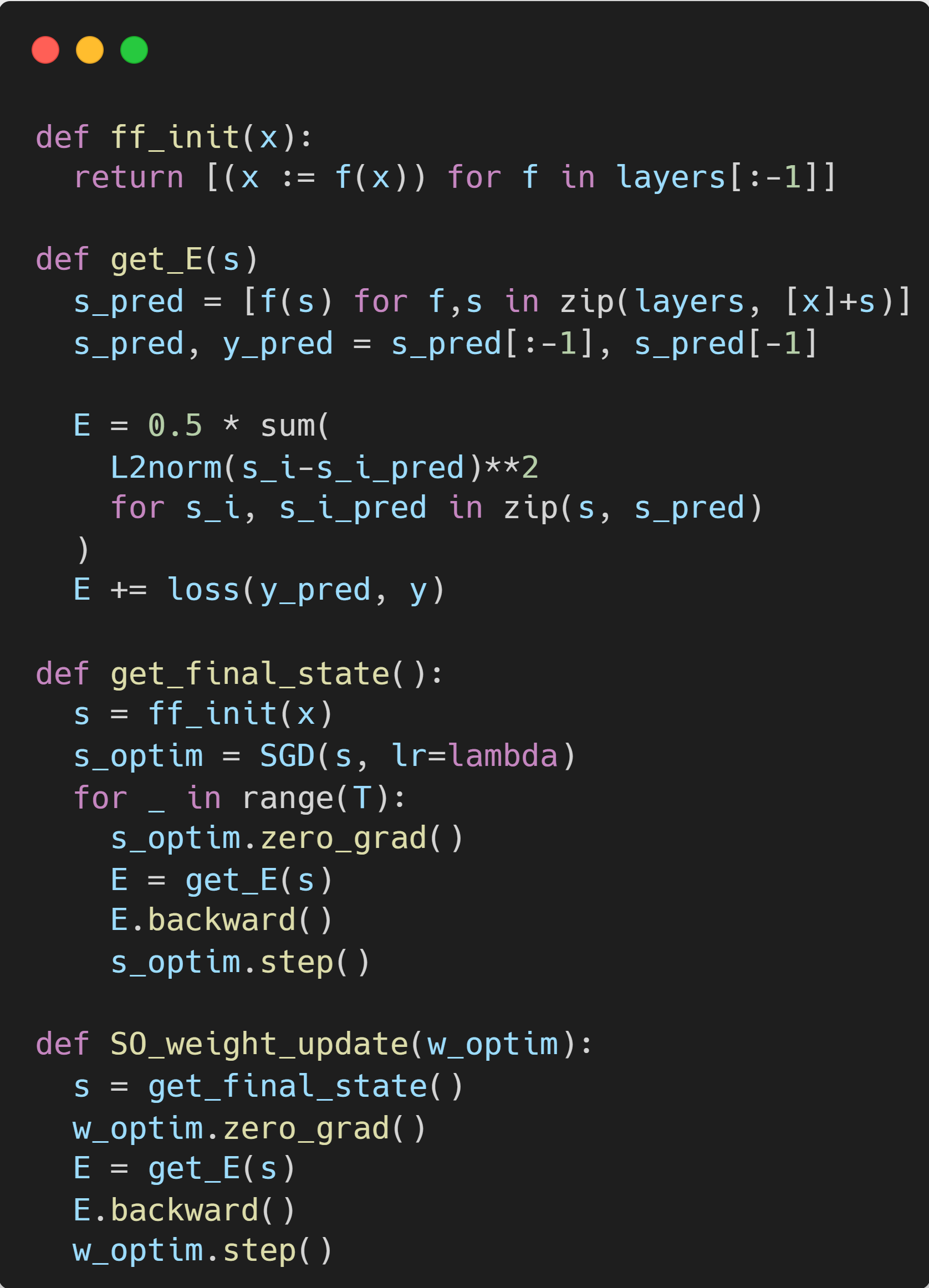
((a)) State Optimization

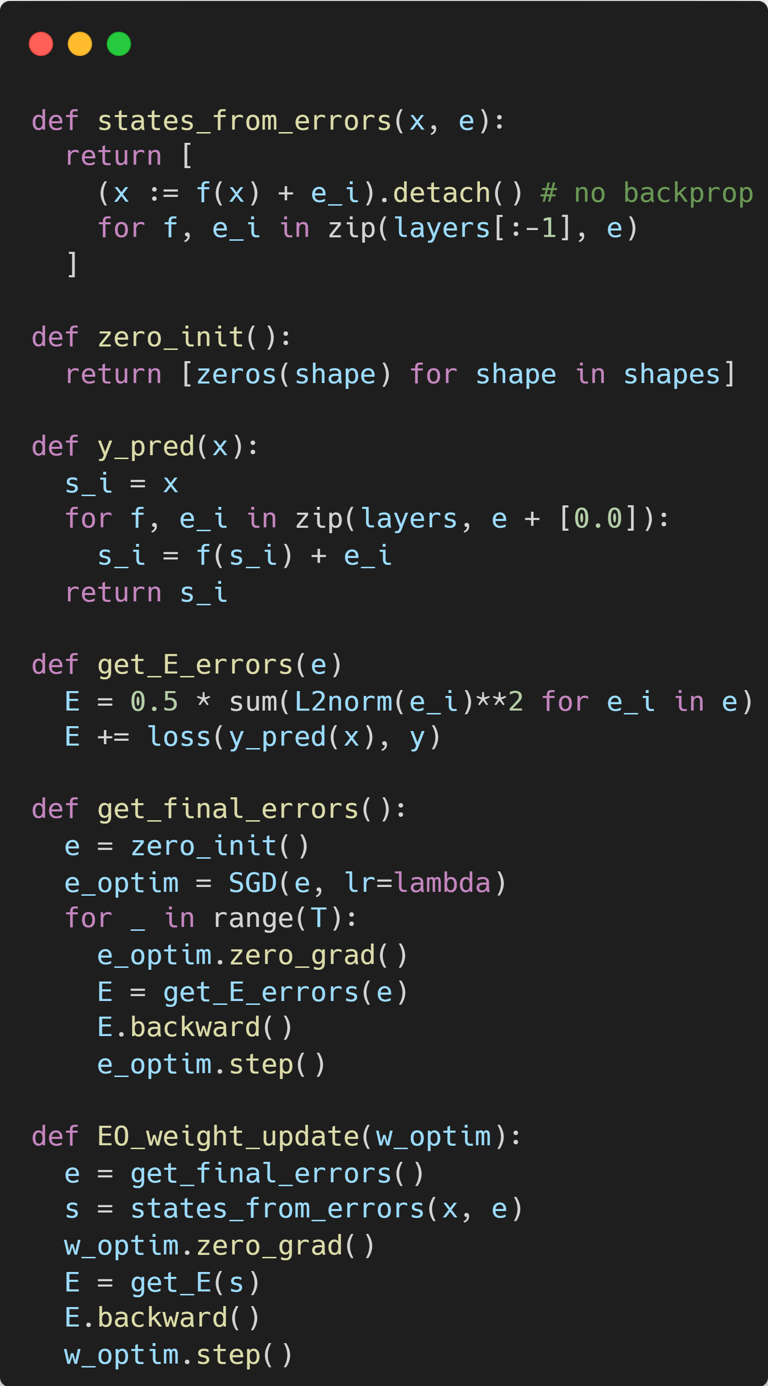
((b)) Error Optimization

Figure A.2: PyTorch-style pseudocode comparison of SO vs. EO

Appendix B Temporal Evolution of States in State Optimization

This appendix extends our analysis of the exponential signal decay phenomenon identified in Section˜3. While the main paper demonstrated how signals attenuate during the initial backward wavefront, we here derive a complete characterization of network dynamics that reveals the underlying mathematical structure governing signal propagation throughout optimization.

Our analysis uncovers a striking connection to Pascal’s triangle, binomial coefficients, and combinatorial signal propagation paths, providing both theoretical insights into the discrete-time nature of the problem and practical understanding of why continuous-time implementations would not suffer from the same limitations.

B.1 Simplified Model for Analytical Tractability

To enable rigorous mathematical analysis, we introduce a simplified model that captures the essential dynamics while remaining analytically tractable.

Key Assumption

After feedforward state initialization, all state predictions $\bm{\hat{s}_{i}}$ remain constant throughout optimization. This assumption implies that signal propagation occurs exclusively in the top-down direction, from output toward input layers.

This simplification provides a reasonable approximation during early-stage optimization, where state dynamics are primarily driven by the output loss $\mathcal{L}$ before significant bottom-up signals emerge. However, it breaks down as the system evolves and predictions begin to change.

Simplified Backward Dynamics

As described in Section˜2, the temporal dynamics of states in SO follow gradient descent on the energy function $E$ with state learning rate $\lambda$:

$$\bm{s_{i}}^{t+1} =\bm{s_{i}}^{t}-\lambda\bm{\nabla}_{\bm{s_{i}}}E^{t}$$

$$=\bm{s_{i}}^{t}-\lambda\bm{\epsilon_{i}}^{t}+\lambda\bm{\epsilon_{i+1}}^{t}\ \frac{\partial\bm{f_{\theta_{i+1}}}}{\partial\bm{s_{i}}}(\bm{s_{i}}^{t}),$$

where $\bm{\epsilon_{i}}:=\bm{s_{i}}-\bm{\hat{s}_{i}}$ represents the layerwise prediction error. Given our key assumption above this is equivalent to the deviation of each layer’s state from its fixed prediction.

To further simplify our analysis, we set $\frac{\partial\bm{f_{\theta_{i+1}}}}{\partial\bm{s_{i}}}(\bm{s_{i}}^{t})\equiv\bm{I}$, reducing the dynamics to:

$$\bm{s_{i}}^{t+1}=\bm{s_{i}}^{t}-\lambda\bm{\epsilon_{i}}^{t}+\lambda\bm{\epsilon_{i+1}}^{t}$$

B.2 Recursive State Dynamics Beyond the Wavefront

Since state predictions $\bm{\hat{s}_{i}}$ remain fixed by assumption, the prediction errors $\bm{\epsilon_{i}}$ follow the same temporal dynamics as the states themselves:

$$\bm{s_{i}}^{t+1} =\bm{s_{i}}^{t}-\lambda\bm{\epsilon_{i}}^{t}+\lambda\bm{\epsilon_{i+1}}^{t}$$

$$\color[rgb]{.5,.5,.5}\iff(\bm{s_{i}}^{t+1}-\bm{\hat{s}_{i}}) \color[rgb]{.5,.5,.5}=(\bm{s_{i}}^{t}-\bm{\hat{s}_{i}})-\lambda\bm{\epsilon_{i}}^{t}+\lambda\bm{\epsilon_{i+1}}^{t}$$

$$\color[rgb]{.5,.5,.5}\iff\bm{\epsilon_{i}}^{t+1} \color[rgb]{.5,.5,.5}=\bm{\epsilon_{i}}^{t}-\lambda\bm{\epsilon_{i}}^{t}+\lambda\bm{\epsilon_{i+1}}^{t}$$

$$\iff\bm{\epsilon_{i}}^{t+1} =(1-\lambda)\bm{\epsilon_{i}}^{t}+\lambda\bm{\epsilon_{i+1}}^{t}$$

For small errors and/or learning rates, we can approximate the magnitude of the right-hand side as the sum of magnitudes, giving rise to recursive dynamics:

$$||\bm{\epsilon_{i}}^{t+1}||\approx(1-\lambda)||\bm{\epsilon_{i}}^{t}||+\lambda||\bm{\epsilon_{i+1}}^{t}||$$

This recursive formula, when traced through the first few time steps, generates a striking pattern. Writing the magnitudes relative to the driving output gradient $\bm{\nabla}_{\!\hat{\bm{y}}}\mathcal{L}$:

The state at time $t=0$ follows from feedforward state initialization, where all internal errors begin at zero. By construction, every entry in the table equals the sum of $(1-\lambda)$ times its left neighbor (its previous value) and $\lambda$ times its upper-left neighbor (influence from the layer above).

B.3 The Binomial Formula for Signal Propagation

Examining the coefficient patterns reveals a fundamental mathematical structure: Pascal’s triangle. We can formalize this behavior with the following binomial formula:

$$||\bm{\epsilon_{L-i}}^{t}||\propto\binom{t}{i}\lambda^{i}(1-\lambda)^{t-i},$$ (4)

where $L$ represents the total number of layers, $i$ is the distance from the output layer, and $t$ denotes the update step. The binomial coefficient $\binom{t}{i}$ encapsulates the number of possible paths through which a signal from the output layer can reach layer $L-i$ within exactly $t$ update steps, given our top-down propagation assumption.

Aside from the initial signal $\bm{\nabla}_{\!\hat{\bm{y}}}\mathcal{L}$ at the output, the formula reveals three additional factors that influence signal magnitude throughout the network:

1. Exponential depth decay $\lambda^{i}$: confirms the exponential attenuation with network depth identified in Section˜3.

2. Temporal decay $(1-\lambda)^{t-i}$: represents the gradual weakening of the original output signal over time, an artifact of our assumption that energy flows exclusively toward lower layers.

3. Different propagation routes $\binom{t}{i}$: accounts for the spatio-temporal variety of signal propagation pathways from output to the current layer.

B.4 State Optimization with High-Precision Simulation

The binomial formula of Eq.˜4 serves as a powerful analytical tool to study SO dynamics without the confounding effects of numerical precision limitations. By implementing this formula directly in logarithmic space using scipy.special.gammaln, we can achieve near-infinite precision and observe the theoretical behavior of signals in SO unhindered by computational constraints.

State Optimization (float64)

Binomial formula ($\infty$-precision)

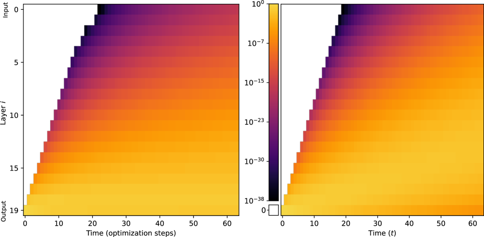
Figure B.1: Evolution of layerwise energies for SO with float64 vs. near-infinite precision (simulated via Eq.˜4). Same setup as in Fig.˜1, described in Section˜D.1.2.

Fig.˜B.1 presents a direct comparison between our high-precision binomial model and a float64 implementation of SO for $\lambda=0.1$. The striking similarity between these plots confirms that our mathematical characterization accurately captures the fundamental early-stage dynamics, despite simplifying assumptions. The orthogonal weight initialization used in our experiments certainly helps here, as it aligns well with our simplified backward dynamics assumption.

Comparing the float64 implementation in Fig.˜B.1 with the float32 version from Fig.˜1 highlights both the importance and limitations of numerical precision in SO. Even with enhanced double-precision floating-point arithmetic, the discontinuous signal propagation persists, though manifesting later and less pronounced.

B.5 Continuous vs. Discrete Time: Limitations of Digital Simulations of State Optimization

While it is clear that numerical precision is the cause of propagation issues in practice, the fundamental source of the exponential signal decay still remains unknown. We hypothesize:

To analyze this claim rigorously, we examine our binomial formula (Eq.˜4) in the continuous-time limit, where $\lambda\rightarrow 0$ (infinitesimal learning rate) and $t\rightarrow\infty$ (continuous updates), with a constant total time $\lambda t$. Setting $t=\tau/\lambda$, we find:

$$\lim_{\lambda\to 0}||\bm{\Delta}\bm{s_{L-i}}^{t=1/\lambda}|| \propto\lim_{\lambda\to 0}\binom{\tau/\lambda}{i}\lambda^{i}(1-\lambda)^{\tau/\lambda-i}$$

$$\approx\lim_{\lambda\to 0}\underbrace{\frac{(\tau/\lambda)^{i}}{i!}}_{\textit{(Stirling's approximation)}}\lambda^{i}\underbrace{e^{-\tau}}_{\textit{(Limit definition of e)}}$$

$$=\frac{\tau^{i}}{i!}e^{-\tau}$$

In the continuous-time limit, our binomial formula transforms into a Poisson distribution, representing the spatial profile of a diffusion process. In this regime, signals diffuse smoothly over time, rather than being subject to the stepwise attenuation seen in discrete updates.

This observation leads to a reassuring conclusion: neuromorphic implementations of SO operating in continuous time would not suffer from the exponential signal decay problem identified in our research. The issue is specific to discrete-time digital implementations subject to both stability constraints and numerical precision limitations. In digital systems, we cannot practically approach the continuous-time limit without incurring prohibitive computational costs.

Therefore, the exponential decay with depth is not an inherent limitation of SO as a theoretical framework but rather a consequence of its discretized formulation for digital hardware. For instance, biological neural systems, operating in continuous time with analog computation, would not face the same fundamental barriers to depth scaling.

B.6 Temporal Scope and Limitations

Our binomial model primarily captures early-stage dynamics but becomes progressively less accurate for extended optimization periods. For longer time horizons, especially with larger learning rates, our assumption of fixed predictions becomes increasingly unrealistic. The model dictates permanent downward energy transmission, moving from output to input, due to a lack of bottom-up signals. In practical implementations, however, layerwise energies will settle across the network in an effort to minimize prediction errors globally. In particular, the output loss $\mathcal{L}$ will generally remain relatively large, even at equilibrium.

Appendix C Further Analyses of Error Optimization

C.1 Theoretical Equivalence of SO and EO

Here, we provide a formal proof of the theoretical equivalence between the SO and EO formulations of PC. We demonstrate that despite their different parameterizations, both approaches converge to identical equilibrium points and represent the same underlying optimization problem.

Bijective Mapping

We first establish a bijective mapping between the optimization variables of SO (the states $\bm{s}$) and EO (the errors $\bm{\epsilon}$).

Theorem C.1 (Bijective Mapping).

For any fixed set of parameters $\bm{\theta}$ and input $\bm{x}$, there exists a bijective mapping between any state configuration $\bm{s}=\{\bm{s_{0}},\bm{s_{1}},\ldots,\bm{s_{L-1}}\}$ in SO and error configuration $\bm{\epsilon}=\{\bm{\epsilon_{0}},\bm{\epsilon_{1}},\ldots,\bm{\epsilon_{L-1}}\}$ in EO.

Proof.

Given states $\bm{s}=\{\bm{s_{0}},\bm{s_{1}},\ldots,\bm{s_{L-1}}\}$ in SO, we can directly compute the corresponding errors:

$$\bm{\epsilon_{i}} =\bm{s_{i}}-\bm{\hat{s}_{i}}=\bm{s_{i}}-\bm{f_{\theta_{i}}}(\bm{s_{i-1}})\quad\text{for}\quad i\in\{0,1,\ldots,L-1\}$$

where for $i=0$, we define $\bm{s_{-1}}:=\bm{x}$ (the input data).

Conversely, given errors $\bm{\epsilon}=\{\bm{\epsilon_{0}},\bm{\epsilon_{1}},\ldots,\bm{\epsilon_{L-1}}\}$ in EO and input $\bm{x}$, we can recursively compute the corresponding states:

$$\bm{s_{0}} =\bm{\hat{s}_{0}}+\bm{\epsilon_{0}}=\bm{f_{\theta_{0}}}(\bm{x})+\bm{\epsilon_{0}}$$

$$\bm{s_{i}} =\bm{\hat{s}_{i}}+\bm{\epsilon_{i}}=\bm{f_{\theta_{i}}}(\bm{s_{i-1}})+\bm{\epsilon_{i}}\quad\text{for}\quad i\in\{1,2,\ldots,L-1\}$$

For a fixed set of parameters $\bm{\theta}$ and input $\bm{x}$, this mapping is one-to-one and onto (i.e., bijective): for any given $\bm{s}$, there is exactly one corresponding $\bm{\epsilon}$, and for any given $\bm{\epsilon}$, there is exactly one corresponding $\bm{s}$. ∎

Energy Function Equivalence

Next, we prove that under this mapping, the energy functions of both formulations are equivalent.

Theorem C.2 (Energy Equivalence).

Under the bijective mapping between $\bm{s}$ and $\bm{\epsilon}$, for any fixed parameter set $\bm{\theta}$ and input-output pair $(\bm{x},\bm{y})$, the energy functions $E_{\text{SO}}(\bm{s},\bm{\theta})$ and $E_{\text{EO}}(\bm{\epsilon},\bm{\theta})$ are identical when evaluated on corresponding configurations.

Proof.

Let us first recall the energy functions for both formulations:

$$E_{\text{SO}}(\bm{s},\bm{\theta}) =\frac{1}{2}\sum_{i=0}^{L-1}\|\bm{s_{i}}-\bm{\hat{s}_{i}}\|^{2}+\mathcal{L}(\hat{\bm{y}},\bm{y})$$

$$E_{\text{EO}}(\bm{\epsilon},\bm{\theta}) =\frac{1}{2}\sum_{i=0}^{L-1}\|\bm{\epsilon_{i}}\|^{2}+\mathcal{L}(\hat{\bm{y}},\bm{y})$$

Starting with $E_{\text{EO}}$ and substituting the definition $\bm{\epsilon_{i}}=\bm{s_{i}}-\bm{\hat{s}_{i}}$:

$$E_{\text{EO}}(\bm{\epsilon},\bm{\theta}) =\frac{1}{2}\sum_{i=0}^{L}\|\bm{\epsilon_{i}}\|^{2}+\mathcal{L}(\hat{\bm{y}},\bm{y})$$

$$=\frac{1}{2}\sum_{i=0}^{L}\|\bm{s_{i}}-\bm{\hat{s}_{i}}\|^{2}+\mathcal{L}(\hat{\bm{y}},\bm{y})$$

$$=E_{\text{SO}}(\bm{s},\bm{\theta})$$

Therefore, the energy functions evaluate to the same value for corresponding configurations of states and errors. ∎

Jacobian of the Transformation

To analyze how gradients and critical points relate between the two formulations, we need the Jacobian matrix of the transformation from errors to states.

Lemma C.3 (Jacobian Structure).

The Jacobian matrix $\textbf{J}=\frac{\partial\bm{s}}{\partial\bm{\epsilon}}$ representing how states change with respect to errors has a lower triangular structure with identity matrices on the diagonal.

Proof.

From the recursive definition of states in terms of errors:

$$\bm{s_{i}} =\bm{f_{\theta_{i}}}(\bm{s_{i-1}})+\bm{\epsilon_{i}}$$

Taking partial derivatives with respect to $\bm{\epsilon_{j}}$:

1. If $j>i$: $\frac{\partial\bm{s_{i}}}{\partial\bm{\epsilon_{j}}}=\mathbf{0}$, since $\bm{s_{i}}$ doesn’t depend on future errors.

2. If $j=i$: $\frac{\partial\bm{s_{i}}}{\partial\bm{\epsilon_{i}}}=\mathbf{I}$, the identity matrix.

3. If $j<i$: $\frac{\partial\bm{s_{i}}}{\partial\bm{\epsilon_{j}}}=\frac{\partial\bm{f_{\theta_{i}}}(\bm{s_{i-1}})}{\partial\bm{s_{i-1}}}\cdot\frac{\partial\bm{s_{i-1}}}{\partial\bm{\epsilon_{j}}}$

Let’s denote $\mathbf{J}_{i}=\frac{\partial\bm{f_{\theta_{i+1}}}(\bm{s_{i}})}{\partial\bm{s_{i}}}$ as the Jacobian of layer $i+1$ with respect to its input (state $i$).

Then we can write:

$$\frac{\partial\bm{s_{i}}}{\partial\bm{\epsilon_{j}}}=\begin{cases}\mathbf{0}&\text{if }j>i\\ \mathbf{I}&\text{if }j=i\\ \mathbf{J}_{i-1}\cdot\frac{\partial\bm{s_{i-1}}}{\partial\bm{\epsilon_{j}}}&\text{if }j<i\end{cases}$$

This recursive structure leads to a lower triangular Jacobian matrix with identity matrices on the diagonal:

$$\textbf{J}=\begin{bmatrix}\mathbf{I}&\mathbf{0}&\mathbf{0}&\cdots&\mathbf{0}\\ \mathbf{J}_{0}&\mathbf{I}&\mathbf{0}&\cdots&\mathbf{0}\\ \mathbf{J}_{1}\mathbf{J}_{0}&\mathbf{J}_{1}&\mathbf{I}&\cdots&\mathbf{0}\\ \vdots&\vdots&\vdots&\ddots&\vdots\\ \prod_{k=0}^{L-1}\mathbf{J}_{k}&\prod_{k=1}^{L-1}\mathbf{J}_{k}&\cdots&\mathbf{J}_{L-1}&\mathbf{I}\end{bmatrix}$$

This structure has important implications: J is invertible with determinant 1, since the determinant of a triangular matrix is the product of its diagonal entries, all of which are 1. ∎

Gradient Equivalence and Critical Points

We now establish the relationship between gradients in both formulations and use it to prove that they share the same critical points.

Theorem C.4 (Gradient Relationship).

The gradients of the energy functions in the SO and EO formulations are related by:

$$\bm{\nabla}_{\bm{\epsilon}}E_{\text{EO}}=\mathbf{J}^{T}\bm{\nabla}_{\bm{s}}E_{\text{SO}}$$

where $\mathbf{J}=\frac{\partial\bm{s}}{\partial\bm{\epsilon}}$ is the Jacobian matrix derived in Lemma C.3.

Proof.

By the chain rule of calculus:

$$\bm{\nabla}_{\bm{\epsilon}}E_{\text{EO}} =\bm{\nabla}_{\bm{\epsilon}}E_{\text{SO}}(\bm{s}(\bm{\epsilon}),\bm{\theta})$$

$$=\left(\frac{\partial\bm{s}}{\partial\bm{\epsilon}}\right)^{T}\bm{\nabla}_{\bm{s}}E_{\text{SO}}$$

$$=\mathbf{J}^{T}\bm{\nabla}_{\bm{s}}E_{\text{SO}}$$

∎

Theorem C.5 (Critical Point Correspondence).

A configuration $\bm{s}^{*}$ is a critical point of $E_{\text{SO}}$ if and only if the corresponding configuration $\bm{\epsilon}^{*}$ is a critical point of $E_{\text{EO}}$.

Proof.

From Theorem C.4, we have:

$$\bm{\nabla}_{\bm{\epsilon}}E_{\text{EO}}=\mathbf{J}^{T}\bm{\nabla}_{\bm{s}}E_{\text{SO}}$$

Since $\mathbf{J}$ is invertible (as shown in Lemma C.3), its transpose $\mathbf{J}^{T}$ is also invertible. Therefore:

$$\bm{\nabla}_{\bm{\epsilon}}E_{\text{EO}}=\mathbf{0}\iff\mathbf{J}^{T}\bm{\nabla}_{\bm{s}}E_{\text{SO}}=\mathbf{0}\iff\bm{\nabla}_{\bm{s}}E_{\text{SO}}=\mathbf{0}$$

This establishes that $\bm{s}^{*}$ is a critical point of $E_{\text{SO}}$ if and only if the corresponding $\bm{\epsilon}^{*}$ is a critical point of $E_{\text{EO}}$. ∎

Local Structure of Critical Points

To complete our proof of optimization equivalence, we need to show that the local structure of critical points (minima, maxima, or saddle points) is preserved between formulations.

Theorem C.6 (Preservation of Local Structure).

A critical point $\bm{s}^{*}$ is a local minimum / maximum / saddle point of $E_{\text{SO}}$ if and only if the corresponding critical point $\bm{\epsilon}^{*}$ is a local minimum / maximum / saddle point of $E_{\text{EO}}$.

Proof.

The local structure of critical points is determined by the eigenvalues of the Hessian matrices:

$$\mathbf{H}_{\bm{s}} =\bm{\nabla}^{2}_{\bm{s}}E_{\text{SO}}$$

$$\mathbf{H}_{\bm{\epsilon}} =\bm{\nabla}^{2}_{\bm{\epsilon}}E_{\text{EO}}$$

To relate these Hessians, we differentiate the relationship in Theorem C.4:

$$\bm{\nabla}_{\bm{\epsilon}}E_{\text{EO}} =\mathbf{J}^{T}\bm{\nabla}_{\bm{s}}E_{\text{SO}}$$

Taking another derivative with respect to $\bm{\epsilon}$:

$$\bm{\nabla}^{2}_{\bm{\epsilon}}E_{\text{EO}} =\frac{\partial}{\partial\bm{\epsilon}}\left(\mathbf{J}^{T}\bm{\nabla}_{\bm{s}}E_{\text{SO}}\right)$$

$$=\frac{\partial\mathbf{J}^{T}}{\partial\bm{\epsilon}}\bm{\nabla}_{\bm{s}}E_{\text{SO}}+\mathbf{J}^{T}\frac{\partial\bm{\nabla}_{\bm{s}}E_{\text{SO}}}{\partial\bm{\epsilon}}$$

$$=\frac{\partial\mathbf{J}^{T}}{\partial\bm{\epsilon}}\bm{\nabla}_{\bm{s}}E_{\text{SO}}+\mathbf{J}^{T}\bm{\nabla}^{2}_{\bm{s}}E_{\text{SO}}\frac{\partial\bm{s}}{\partial\bm{\epsilon}}$$

$$=\frac{\partial\mathbf{J}^{T}}{\partial\bm{\epsilon}}\bm{\nabla}_{\bm{s}}E_{\text{SO}}+\mathbf{J}^{T}\mathbf{H}_{\bm{s}}\mathbf{J}$$

At a critical point where $\bm{\nabla}_{\bm{s}}E_{\text{SO}}=\mathbf{0}$, the first term vanishes, giving:

$$\mathbf{H}_{\bm{\epsilon}}=\mathbf{J}^{T}\mathbf{H}_{\bm{s}}\mathbf{J}$$

This establishes that $\mathbf{H}_{\bm{\epsilon}}$ and $\mathbf{H}_{\bm{s}}$ are congruent matrices, considering $\mathbf{J}$ is invertible.

By Sylvester’s law of inertia, congruent matrices have the same number of positive, negative, and zero eigenvalues. Therefore:

• $\mathbf{H}_{\bm{s}}$ is positive definite (all eigenvalues positive) if and only if $\mathbf{H}_{\bm{\epsilon}}$ is positive definite

• $\mathbf{H}_{\bm{s}}$ is negative definite (all eigenvalues negative) if and only if $\mathbf{H}_{\bm{\epsilon}}$ is negative definite

• $\mathbf{H}_{\bm{s}}$ has mixed positive/negative eigenvalues (saddle point) if and only if $\mathbf{H}_{\bm{\epsilon}}$ has the same eigenvalue signature

This preserves the classification of critical points as local minima, maxima, or saddle points between the two formulations. ∎

Dynamical Systems Analysis

While the energy functions and their critical points are identical, the optimization dynamics differ significantly due to the reparameterization.

Theorem C.7 (Dynamical Equivalence).

The continuous-time dynamics in SO and EO both converge to the same equilibrium points, but follow different trajectories in their respective spaces.

Proof.

Under the notation $\dot{\bm{x}}:=\frac{d\bm{x}}{dt}$, the continuous-time dynamics for both formulations are:

$$\text{SO:}\quad\dot{\bm{s}} =-\bm{\nabla}_{\bm{s}}E_{\text{SO}}$$

$$\text{EO:}\quad\dot{\bm{\epsilon}} =-\bm{\nabla}_{\bm{\epsilon}}E_{\text{EO}}$$

Using the relation $\bm{\nabla}_{\bm{\epsilon}}E_{\text{EO}}=\mathbf{J}^{T}\bm{\nabla}_{\bm{s}}E_{\text{SO}}$, the EO dynamics can be rewritten as:

$$\dot{\bm{\epsilon}} =-\mathbf{J}^{T}\bm{\nabla}_{\bm{s}}E_{\text{SO}}$$

To compare these dynamics in the same space, we need to transform $\dot{\bm{\epsilon}}$ to $\dot{\bm{s}}$. Using the chain rule:

$$\dot{\bm{s}} =\frac{\partial\bm{s}}{\partial\bm{\epsilon}}\dot{\bm{\epsilon}}$$

$$=\mathbf{J}\dot{\bm{\epsilon}}$$

$$=-\mathbf{J}\mathbf{J}^{T}\bm{\nabla}_{\bm{s}}E_{\text{SO}}$$

Comparing with the SO dynamics:

$$\dot{\bm{s}}_{SO} =-\bm{\nabla}_{\bm{s}}E_{\text{SO}}$$

$$\dot{\bm{s}}_{EO} =-\mathbf{J}\mathbf{J}^{T}\bm{\nabla}_{\bm{s}}E_{\text{SO}}$$

The difference is the matrix $\mathbf{J}\mathbf{J}^{T}$, which acts as a preconditioner for the gradient descent. This matrix is positive definite (since $\mathbf{J}$ has full rank), meaning that the EO dynamics will always move in a descent direction for $E_{\text{SO}}$, but with a different step size and direction than SO.

Both dynamical systems will converge to the same equilibrium points where $\bm{\nabla}_{\bm{s}}E_{\text{SO}}=\mathbf{0}$, but will follow different trajectories to get there. ∎

Global Connectivity and Signal Propagation

The key computational advantage of EO over SO lies in its global connectivity structure. This difference affects how signals propagate through the network.

Theorem C.8 (Signal Propagation).

In the SO formulation, signals propagate sequentially through the network layers, resulting in exponential decay with network depth. In contrast, EO allows direct signal propagation to all layers simultaneously, eliminating the signal decay problem.

Proof.

In SO, the state update equations are:

$$\dot{\bm{s_{i}}} =-\bm{\nabla}_{\bm{s_{i}}}E_{\text{SO}}$$

$$=-\bm{\epsilon_{i}}+\bm{\epsilon_{i+1}}\ \frac{\partial\bm{f_{\theta_{i+1}}}}{\partial\bm{s_{i}}}(\bm{s_{i}})$$

The crucial observation is that $\dot{\bm{s_{i}}}$ depends only on errors from adjacent layers ($\bm{\epsilon_{i}}$ and $\bm{\epsilon_{i+1}}$). This local connectivity means that a signal from the output layer ($\bm{\nabla}_{\hat{\bm{y}}}\mathcal{L}$) must propagate through all intermediate layers to reach the input layer, attenuating at each step.

In EO, by contrast, the gradient is computed through the entire computational graph:

$$\dot{\bm{\epsilon_{i}}} =-\bm{\nabla}_{\bm{\epsilon_{i}}}E_{\text{EO}}$$

$$=-\bm{\epsilon_{i}}-\frac{\partial\hat{\bm{y}}}{\partial\bm{\epsilon_{i}}}^{T}\bm{\nabla}_{\hat{\bm{y}}}\mathcal{L}$$

$$\text{with}\qquad\frac{\partial\hat{\bm{y}}}{\partial\bm{\epsilon_{i}}}=\frac{\partial\hat{\bm{y}}}{\partial\bm{\epsilon_{L-1}}}\cdot\frac{\partial\bm{\epsilon_{L-1}}}{\partial\bm{\epsilon_{L-2}}}\cdot\ldots\cdot\frac{\partial\bm{\epsilon_{i+1}}}{\partial\bm{\epsilon_{i}}}$$

Hence, $\dot{\bm{\epsilon_{i}}}$ directly depends on all errors from layer $i$ to $L$. This global connectivity allows signals from the output layer to immediately affect all earlier layers, eliminating the signal decay problem.

The mathematical consequence of this difference is that in SO, the influence of the output error on layer $i$ decreases exponentially with the distance from the output (as explained extensively in Section˜3), while in EO, this influence is direct and unattenuated. ∎

Limitations and Caveats

While the two formulations are theoretically equivalent in terms of equilibrium points, several practical considerations affect their performance:

1. Optimization Landscape: The different parameterizations create different optimization trajectories that may encounter different local minima under stochastic optimization.

2. Numerical Stability: The formulations may exhibit different numerical properties, particularly with respect to hyperparameter sensitivity and discretization effects. For instance, in Section˜3, the numerical issues of State Optimization are highlighted.

3. Implementation Efficiency: The global connectivity of EO imposes different computational demands than the local connectivity of SO, affecting implementation efficiency on different hardware architectures. On GPU, the backpropagation algorithm behind EO is highly efficient, despite being sequential. However, the local and parallel nature of SO enables a far more efficient neuromorphic implementation.

Despite these practical differences, our theoretical equivalence analysis confirms that EO is a valid reparameterization of PC that preserves its fundamental principles while offering significant computational advantages for deep networks.

C.2 Exact Backpropagation using Error Optimization

Below, we explore an important theoretical property of EO: under specific conditions, EO can become mathematically equivalent to standard backpropagation. This relationship deserves careful examination, as it affects how researchers implement and interpret EO results.

C.2.1 When EO Reduces to Backpropagation

The use of backpropagation within EO’s computational structure naturally raises the question of when the two methods become mathematically equivalent. We demonstrate that EO reduces to standard backpropagation under specific conditions.

Proof.

We consider each case separately, proving their equivalence to backpropagation.

Case 1: Single Optimization Step ($T=1$)
With a single update step, the error variables are updated to:

$$\bm{\epsilon_{i}}=-\lambda\bm{\nabla}_{\bm{\epsilon_{i}}}\mathcal{L}(\hat{\bm{y}},\bm{y})$$

The subsequent parameter update becomes:

$$\Delta\bm{\theta_{i}} \propto-\frac{\partial\bm{\hat{s}_{i}}}{\partial\bm{\theta_{i}}}^{T}\bm{\epsilon_{i}}$$

$$=\lambda\frac{\partial\bm{\hat{s}_{i}}}{\partial\bm{\theta_{i}}}^{T}\underbrace{\frac{\partial\bm{s_{i}}}{\partial\bm{\hat{s}_{i}}}^{T}}_{=\bm{I}}\underbrace{\frac{\partial\bm{\epsilon_{i}}}{\partial\bm{s_{i}}}^{T}}_{=\bm{I}}\bm{\nabla}_{\bm{\epsilon_{i}}}\mathcal{L}(\hat{\bm{y}},\bm{y})$$

$$=\lambda\bm{\nabla}_{\bm{\theta_{i}}}\mathcal{L}(\hat{\bm{y}},\bm{y})$$

This is precisely the gradient update rule used in standard backpropagation, scaled by the learning rate $\lambda$.

Case 2: Small Learning Rate ($\lambda\ll 1/T$)
For a small error learning rate $\lambda$, after $T$ optimization steps, the error can be approximated as a linear accumulation of $T$ identical updates:

$$\bm{\epsilon_{i}}\approx-\lambda T\bm{\nabla}_{\bm{\epsilon_{i}}}\mathcal{L}(\hat{\bm{y}},\bm{y})$$

Following the same reasoning as for case 1, the resulting parameter update now becomes:

$$\Delta\bm{\theta_{i}}\propto\lambda T\bm{\nabla}_{\bm{\theta_{i}}}\mathcal{L}(\hat{\bm{y}},\bm{y})$$

This approximation holds when $\lambda T$ remains sufficiently small, such that the error-perturbed output prediction $\hat{\bm{y}}$ of EO still closely approximates the unperturbed feedforward prediction $\hat{\bm{y}}$ of backprop. ∎

C.2.2 Experimental Considerations

In our experiments, we found that smaller values of $\lambda T$ generally performed best. However, we deliberately maintained this value above the threshold that would cause EO to reduce to regular backpropagation. Complete experimental details are provided in Appendix˜D.

C.2.3 Contrast with State Optimization

This situation differs notably from SO, which can also become equivalent to backpropagation under certain conditions [48, 51]. However, these conditions typically involve specific algorithmic tweaks that rarely occur in practice, thereby protecting SO implementations from accidentally reducing to backpropagation.

EO, by contrast, presents a more subtle boundary. During hyperparameter tuning, one might inadvertently select learning rates and iteration counts that effectively transform EO into standard backpropagation. Researchers working with EO should therefore carefully monitor these parameters to ensure they are truly studying PC dynamics rather than rediscovering backpropagation in disguise.

C.3 Details of Deep Linear Network Trained on MNIST

Below, we briefly summarize the technical details needed to reproduce Fig.˜5. Specifically, we used the following architecture:

• Number of layers: 20

  • Specifically: $\bm{x}-\bm{s_{0}}-\bm{s_{1}}-\dots-\bm{s_{8}}-\bm{s_{9}}-\bm{s_{10}}-\dots-\bm{s_{17}}-\bm{s_{18}}-\bm{y}$

• Hidden state dim: 128

• Activation function: None (not even at the output)

• Weight init: orthogonal (linear gain) [47]

• Bias init: zero

• State/error optimizer: SGD

• Pretraining

  • Weight optimizer: Adam [37]

  • Weight learning rate: 0.001 (not tuned for this proof-of-concept)

  • Gradient algorithm: Backpropagation (fast, stable, and neutral w.r.t. SO & EO)

  • Dataset: EMNIST-MNIST [42]

  • Batch size: 64

  • Epochs: 2

  • Final test accuracy: 84.5%

For a fair comparison between State Optimization and Error Optimization, we tuned the internal learning rate for both, with the objective of maximum convergence to the analytical optimum:

• Error Optimization

  • e_lr sweep: {0.001, 0.005, 0.01, 0.05, 0.1}

  • Optimal e_lr: 0.05

  • #iters: 256

• State Optimization

  • s_lr sweep: {0.05, 0.1, 0.3, 0.5}

  • Optimal s_lr: 0.3

  • #iters: 4096

The analytical solution was obtained via sparse matrix inversion using scipy.sparse.linalg.spsolve.

Note: Fig.˜5 shows state dynamics for both State Optimization and Error Optimization. To get states for the latter, we project from errors to states at every time step.

C.4 State Dynamics in Non-Linear Models Trained on MNIST

Building on our analysis of linear models in Section 4.3, we extend our investigation to the more practical scenario of non-linear networks. This extension allows us to evaluate whether the signal propagation advantages of EO generalize beyond the analytically tractable linear case.

C.4.1 Experimental Setup

We employed the 20-layer “Deep MLP” architecture detailed in Appendix˜D, pretrained on MNIST using one of two different loss functions: squared error and cross-entropy. Unlike the linear models, these non-linear networks achieve higher test accuracy (95% vs. 85%), representing a more realistic training scenario. However, this improved performance introduces an important methodological consideration: since analytical solutions are unavailable for non-linear models, we must turn to EO’s convergence state as our reference equilibrium point. This choice inherently favors EO and should be considered when interpreting results.

C.4.2 Impact of Loss Function and Input Difficulty

As pointed out in Section˜3, the signal decay problem of SO depends critically on the output gradient $\bm{\nabla}_{\hat{\bm{y}}}\mathcal{L}$. In well-trained non-linear models, the loss—and hence its gradient—can become extremely small for easily classified examples, leading to even worse signal propagation issues. To investigate this effect systematically, we varied both the loss function (squared error vs. cross-entropy) and input difficulty (easy vs. hard-to-classify images). All experiments were implemented with float64 precision to ensure numerical stability and avoid precision-related confounders in the convergence analysis.

	Squared Error Loss	Cross-Entropy Loss
Easy image
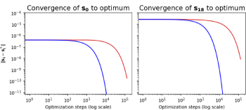
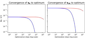
Hard image

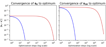
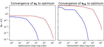
Figure C.1: Convergence dynamics in 20-layer PC-MLPs trained on MNIST with float64 precision. For easily-classified inputs (marked by near-zero loss), gradient signals become prohibitively small, hindering convergence. Error Optimization consistently outperforms State Optimization by orders of magnitude across all conditions.

Fig.˜C.1 presents the convergence dynamics for both SO and EO across these conditions. Several important observations emerge from these experiments:

1. Performance across loss functions: Cross-entropy loss appears to create a more challenging optimization landscape for both SO and EO, despite its generally more favorable gradient properties compared to squared error. However, the smaller gradient signals from squared error do lead to long propagation delays in SO, requiring almost 1000 update steps to progress just a single layer and reach $\bm{s_{18}}$.

2. Input difficulty effects: For highly accurate models, most inputs will be “easy” (classified with high confidence), thereby generating minimal loss gradients. This greatly hinders overall signal propagation, even for EO in our float64 simulations. By contrast, “hard” inputs (resulting in larger gradients) greatly accelerate EO, while modestly improving SO’s convergence speed.

3. Overall convergence speed: EO consistently converges orders of magnitude faster than SO across all experimental conditions. This advantage is most pronounced with squared error loss on hard images (bottom left panel), where EO converges approximately 10,000 times faster than SO for the exact same model.

4. Identical equilibria: Even in the non-linear case, SO and EO seem to head towards the same equilibrium points, highlighting their equivalence as established in Section˜C.1. Note that this is not necessarily true for all model architectures and datasets, as spurious local minima may affect SO and EO in different ways.

5. Practical implications: Perhaps most critically, SO requires an impractical number of update steps (>100,000) to reach convergence in these non-linear networks, underscoring the practical importance of our EO reformulation for deep PC architectures.

These findings extend and reinforce the convergence analysis presented in Section˜4.3. They confirm that the advantages of EO’s global connectivity structure generalize from the analytically tractable linear case to practical non-linear networks with different loss functions.

Appendix D Overview of Experimental Implementation Details

In this appendix, we provide all details necessary to reproduce our experimental results from Table˜1. Furthermore, we perform additional experiments on a 20-layer deep MLP architecture, which was used for Figs.˜1 and C.1.

Our code is available at https://github.com/cgoemaere/pc_error_optimization.

D.1 MLPs on MNIST & FashionMNIST

Compute resources

• CPU: Intel Xeon E5-2620 v4

• RAM: 32 GiB

• GPU: NVIDIA GeForce GTX 1080 Ti

• Compute time per experiment: (without early stopping or failure)

  • MNIST - MLP:

    • Error Optim: 10min (#iters=4, 25 epochs) – 1h (#iters=256, 5 epochs)

    • State Optim: 10min (#iters=4, 25 epochs) – 45min (#iters=256, 5 epochs)

    • Backprop: 2-7min

  • MNIST - Deep MLP:

    • Error Optim: 12min (#iters=4, 25 epochs) – 3h (#iters=256, 5 epochs)

    • State Optim: 25min (#iters=4, 25 epochs) – 3h (#iters=256, 5 epochs)

    • Backprop: 2-8min

  • FashionMNIST - MLP:

    • Error Optim: 6min (#iters=4, 14 epochs) – 14min (#iters=64, 5 epochs)

    • State Optim: 13min (#iters=16, 14 epochs) – 45min (#iters=256, 5 epochs)

    • Backprop: 3-7min

  • FashionMNIST - Deep MLP:

    • Error Optim: 20min (#iters=4, 17 epochs) – 45min (#iters=64, 5 epochs)

    • State Optim: 1h (#iters=64, 7 epochs) – 5h30 (#iters=256, 13 epochs)

    • Backprop: 4-7min

• Total compute time estimate:

  • MNIST: $\pm$150h

  • FashionMNIST: $\pm$150h

Architecture

• Number of layers: 4 (MLP), 20 (Deep MLP; see below)

• Hidden state dim: 128

• Activation function: GELU [40] (+ Sigmoid for MSE loss)

• Weight init: orthogonal (with ReLU gain) [47]

• Bias init: zero

• Pseudorandom seed: 42 for hyperparameter sweep, {0, 1, 2, 3, 4} for final test accuracy over 5 seeds. We set the seed using lightning.seed_everything(workers=True) before any data or weight initialization.

• State/error optimizer: SGD

• Weight optimizer: Adam [37]

D.1.1 Additional Experiments on Deep MLPs

Table D.1: Additional test accuracies (in %) of EO, SO and backprop for a deep MLP architecture. Bold indicates best results within confidence intervals (mean ± 1 std. dev.; taken over 5 seeds).

Loss $\mathcal{L}$	Mean Squared Error			Cross-Entropy
Training algorithm	EO	SO	Backprop	EO	SO	Backprop
Deep MLP (20 layers)
MNIST	$97.11^{\pm 0.39}$	$96.89^{\pm 0.33}$	$\mathbf{97.89^{\pm 0.15}}$	$94.84^{\pm 0.54}$	$95.23^{\pm 1.24}$	$\mathbf{97.20^{\pm 0.07}}$
FashionMNIST	$\mathbf{85.04^{\pm 2.94}}$	$84.92^{\pm 0.40}$	$\mathbf{87.91^{\pm 0.45}}$	$81.37^{\pm 0.40}$	$79.95^{\pm 1.62}$	$\mathbf{87.78^{\pm 0.18}}$

As an addition to the benchmark of [62], we evaluated the performance for a 20-layer deep version of the MLP. As this architecture presents training challenges even with backpropagation, we turned to orthogonal weight initialization for enhanced stability [47]. The results are stated in Table˜D.1.

Despite our expectation of a large performance gap, both EO and SO performed similarly. We hypothesize that orthogonal initialization may ease the signal decay problem by maintaining eigenvalues close to 1, thereby creating an unexpectedly strong baseline. This suggests that careful weight initialization can mitigate some of SO’s inherent optimization challenges. However, this strategy is less applicable to convolutional architectures, where the performance difference between EO and SO remains substantial.

To avoid confusion, we decided to move these results to appendix, rather than state them in Section˜5.

D.1.2 Details of Figure 1

Below, we provide all details necessary to reproduce Fig.˜1. Above all, our goal was to illustrate the problem of signal decay under realistic conditions.

The model is an untrained Deep MLP + Cross-Entropy, as detailed above. We track the layerwise energies across optimization for a single MNIST data pair $(\bm{x},\bm{y})$. These are calculated using the energy functions corresponding to SO and EO (shown side-by-side in Fig.˜2). We perform 64 optimization steps for SO and 8 for EO, both with a learning rate $\lambda=0.1$.

D.1.3 MNIST

Data

We used EMNIST-MNIST [42], which is a well-documented reproduction of the original MNIST dataset [33]. The images are first rescaled to the range [0, 1], then they are normalized using the fixed values mean=0.5 and std=0.5 [62, same as]. We set the batch size constant at 64. The validation set was 10% of the training data, split randomly but with a fixed seed. For final test performance, we don’t split a separate validation set, but simply train on the whole training set.

Error Optimization

First, we did a hyperparameter sweep over the inner optimization hyperparameters (error learning rate (e_lr) and number of update steps (#iters)), with the weight learning rate (w_lr) constant at 3e-4 (or 3e-5 for Deep MLP+CE). During these sweeps, we train for 5 epochs. Then, we fixed the best inner optimization hyperparameters for each setting, and tuned w_lr and the number of epochs by means of early stopping, with a maximum of 25 epochs. See Table˜D.2 for more details of the sweep.

Table D.2: Hyperparameter sweep intervals and optimal values for EO-MLPs on MNIST

Hyperparams	Sweep values	MLP+MSE	MLP+CE	Deep MLP+MSE	Deep MLP+CE
e_lr	{0.001, 0.005, 0.01, 0.05, 0.1, 0.5}	0.05	0.001	0.001	0.001
#iters	{4, 16, 64, 256}	4	4	4	4
w_lr	{1e-5, 3e-5, 5e-5, 1e-4, 3e-4, 5e-4, 1e-3}	1e-4	1e-4	1e-4	1e-5
#epochs	Early Stopping(patience=3), up to 25	25	20	14	25

State Optimization

First, we did a hyperparameter sweep over the inner optimization hyperparameters (state learning rate (still denoted as e_lr for implementation purposes) and number of update steps (#iters)), with the weight learning rate (w_lr) constant at 1e-4 (the optimal rate for EO). During these sweeps, we train for 5 epochs. Then, we fixed the best inner optimization hyperparameters for each setting, and tuned w_lr and the number of epochs by means of early stopping, with a maximum of 25 epochs. See Table˜D.3 for more details of the sweep.

Table D.3: Hyperparameter sweep intervals and optimal values for SO-MLPs on MNIST

Hyperparams	Sweep values	MLP+MSE	MLP+CE	Deep MLP+MSE	Deep MLP+CE
e_lr	{0.01, 0.03, 0.1, 0.3}	0.01	0.03	0.3	0.3
#iters	{4, 16, 64, 256}	16	4	64	64
w_lr	{3e-5, 5e-5, 1e-4, 3e-4, 5e-4, 1e-3}	1e-4	1e-4	1e-4	5e-5
#epochs	Early Stopping(patience=3), up to 25	25	21	12	15

Backprop

Since there is no inner optimization in backprop, we simply tuned w_lr and the number of epochs by means of early stopping, with a maximum of 25 epochs. See Table˜D.4 for all details.

Table D.4: Hyperparameter sweep intervals and optimal values for backprop-MLPs on MNIST

Hyperparams	Sweep values	MLP+MSE	MLP+CE	Deep MLP+MSE	Deep MLP+CE
w_lr	{3e-5, 5e-5, 1e-4, 3e-4, 5e-4, 1e-3}	3e-4	1e-4	3e-4	5e-5
#epochs	Early Stopping(patience=3), up to 25	16	20	22	18

D.1.4 FashionMNIST

Data

We used the FashionMNIST dataset [44]. The images are first rescaled to the range [0, 1], then they are normalized using the fixed values mean=0.5 and std=0.5 [62, same as]. We set the batch size constant at 64. The validation set was 10% of the training data, split randomly but with a fixed seed. For final test performance, we don’t split a separate validation set, but simply train on the whole training set.

Error Optimization

First, we did a hyperparameter sweep over the inner optimization hyperparameters (error learning rate (e_lr) and number of update steps (#iters)), with the weight learning rate (w_lr) constant at 1e-4 (3e-5 for Deep MLP+CE). During these sweeps, we train for 5 epochs. Then, we fixed the best inner optimization hyperparameters for each setting, and tuned w_lr and the number of epochs by means of early stopping, with a maximum of 25 epochs. See Table˜D.5 for more details of the sweep.

Table D.5: Hyperparameter sweep intervals and optimal values for EO-MLPs on FashionMNIST

Hyperparams	Sweep values	MLP+MSE	MLP+CE	Deep MLP+MSE	Deep MLP+CE
e_lr	{0.001, 0.003, 0.01, 0.03, 0.1}	0.01	0.003	0.001	0.001
#iters	{4, 16, 64}	16	4	4	4
w_lr	{3e-5, 5e-5, 1e-4, 3e-4}	5e-5	5e-5	3e-4	3e-5
#epochs	Early Stopping(patience=3), up to 25	12	14	17	2

State Optimization

First, we did a hyperparameter sweep over the inner optimization hyperparameters (state learning rate (still denoted as e_lr for implementation purposes) and number of update steps (#iters)), with the weight learning rate (w_lr) constant at 1e-4. During these sweeps, we train for 5 epochs. Then, we fixed the best inner optimization hyperparameters for each setting, and tuned w_lr and the number of epochs by means of early stopping, with a maximum of 25 epochs. See Table˜D.6 for more details of the sweep.

Table D.6: Hyperparameter sweep intervals and optimal values for SO-MLPs on FashionMNIST

Hyperparams	Sweep values	MLP+MSE	MLP+CE	Deep MLP+MSE	Deep MLP+CE
e_lr	{0.01, 0.03, 0.1, 0.3}	0.03	0.01	0.3	0.1
#iters	{4, 16, 64, 256}	64	16	64	256
w_lr	{3e-5, 5e-5, 1e-4, 3e-4}	1e-4	1e-4	5e-5	3e-5
#epochs	Early Stopping(patience=3), up to 25	14	14	7	/

Backprop

Since there is no inner optimization in backprop, we simply tuned w_lr and the number of epochs by means of early stopping, with a maximum of 25 epochs. See Table˜D.7 for all details.

Table D.7: Hyperparameter sweep intervals and optimal values for BP-MLPs on FashionMNIST

Hyperparams	Sweep values	MLP+MSE	MLP+CE	Deep MLP+MSE	Deep MLP+CE
w_lr	{3e-5, 5e-5, 1e-4, 3e-4}	3e-4	1e-4	1e-4	3e-4
#epochs	Early Stopping(patience=3), up to 25	15	25	17	10

D.2 VGG-models and ResNet-18

Compute resources

We report the resources used for training and each model’s training time. The training times required for a model with MSE or CE loss are comparable. For hyperparameter tuning, we evaluate 200 distinct parameter configurations, making the total computational cost approximately 200 times greater than that of a single training run.

• CPU: Intel Xeon w5-3423

• RAM: 197 GiB

• GPU: NVIDIA RTX A6000

• Compute time per experiment: (without early stopping or failure)

  Dataset	Model	Error Optim	State Optim	Backprop
  CIFAR-10	VGG-5	6min	9min	2min
  	VGG-7	7min	11min	2min
  	VGG-9	9min	17min	3min
  	ResNet-18	29min	–	6min
  CIFAR-100	VGG-5	6min	9min	2min
  	VGG-7	7min	12min	2min
  	VGG-9	9min	19min	3min
  	ResNet-18	29min	–	6min

• Total compute time estimate for tuning across model architecture and loss function:

  • Error Optim: $\pm$680h

  • State Optim: $\pm$510h

  • Backprop: $\pm$170h

Data

We used the CIFAR-10/100 datasets [35]. The images are first rescaled to the range [0, 1], then they are normalized with the mean and standard deviation given in Table˜D.8 [62, same as]. We set the batch size constant at 256. The validation set was 5% of the training data, split randomly but with a fixed seed. For final test performance, we don’t split a separate validation set, but simply train on the whole training set.

Table D.8: Data normalization

	Mean ($\mu$)	Std ($\sigma$)
CIFAR-10	[0.4914, 0.4822, 0.4465]	[0.2023, 0.1994, 0.2010]
CIFAR-100	[0.5071, 0.4867, 0.4408]	[0.2675, 0.2565, 0.2761]

VGG architecture

VGG models are deep convolutional neural networks [38]. Table˜D.9 provides a detailed summary of the model architectures used for the VGG-5, VGG-7 and VGG-9 models. After the convolutional layers, a single linear layer produces a class prediction. The activation function of the models was selected from among ReLU, Tanh, Leaky ReLU, and GELU [40] during model tuning.

Table D.9: Detailed architectures of VGG models. The locations of the pooling layers correspond to the indices of the convolutional layers after which the max-pooling operations are applied.

	VGG-5	VGG-7	VGG-9
Channel Sizes	[128, 256, 512, 512]	[128, 128, 256, 256, 512, 512]	[128, 128, 256, 256, 512, 512, 512, 512]
Kernel Sizes	[3, 3, 3, 3]	[3, 3, 3, 3, 3, 3]	[3, 3, 3, 3, 3, 3, 3, 3]
Strides	[1, 1, 1, 1]	[1, 1, 1, 1, 1, 1]	[1, 1, 1, 1, 1, 1, 1, 1]
Paddings	[1, 1, 1, 1]	[1, 1, 1, 0, 1, 0]	[1, 1, 1, 1, 1, 1, 1, 1]
Pool location	[0, 1, 2, 3]	[0, 2, 4]	[0, 2, 4, 6]
Pool window	2 × 2	2 × 2	2 × 2
Pool stride	2	2	2

ResNet-18 architecture

The ResNet-18 model is a convolutional neural network with skip connections [39]. Our implementation follows the standard ResNet-18 architecture with modifications tailored for CIFAR-10/100. It is composed of an initial convolutional stem followed by four residual stages, each consisting of two residual blocks. Each residual block comprises two 3×3 convolutional layers with batch normalization and ReLU activation, followed by an identity shortcut connection. Spatial downsampling is performed via stride-2 convolutions at the beginning of each stage beyond the first. Table˜D.10 details the layer configuration.

Table D.10: ResNet-18 architecture adapted for CIFAR-10/100 image classification. The feature shape describes the image height and width after each stage. The residual configuration gives the dimension of the convolution mask, the number of channels and the stride used for the residual stream. All the convolutional layers used a padding of one, and each convolution was followed by a batch normalisation layer. Stages one to four include skip connections for every residual.

Stage	Feature shape	Residual configuration
Conv Stem	$32\times 32$	Conv3x3, 64, $\text{stride}=1$
Stage 1	$32\times 32$	$\begin{bmatrix}\text{Conv3x3},64,\text{stride}=1\\ \text{Conv3x3},64,\text{stride}=1\end{bmatrix}\times 2$
Stage 2	$16\times 16$	$\begin{bmatrix}\text{Conv3x3},128,\text{stride}=2\\ \text{Conv3x3},128,\text{stride}=1\end{bmatrix}\times 2$
Stage 3	$8\times 8$	$\begin{bmatrix}\text{Conv3x3},256,\text{stride}=2\\ \text{Conv3x3},256,\text{stride}=1\end{bmatrix}\times 2$
Stage 4	$4\times 4$	$\begin{bmatrix}\text{Conv3x3},512,\text{stride}=2\\ \text{Conv3x3},512,\text{stride}=1\end{bmatrix}\times 2$
Head	$1\times 1$	Global AvgPool + Linear classifier

Learning rate schedule

The following learning rate schedule was used to help stabilize training:

1. For the first 10% of training, the learning rate increases linearly from w_lr up to 1.1$\times$w_lr.

2. After the warmup phase, a cosine decay is applied. The learning rate smoothly decreases to 0.1$\times$w_lr, following a cosine curve, for the remaining training steps.

Weight initialization

We used the default PyTorch weight initialization, which amounts to a random uniform weight and bias initialization. For pseudorandom seeds, we use 42 for the hyperparameter sweeps, and {0, 1, 2, 3, 42} for the final test accuracy over 5 seeds. We set the seed using lightning.seed_everything(workers=True) before any data or weight initialization.

Table D.11: Summary of hyperparameter tuning and training settings for convolutional models

Method	Tuned hyperparameter range	Optimizer	Optim steps (T)	Epochs (sweep/final)
EO	e_lr: fixed at 0.001 e_momentum: fixed at 0.0 w_lr: log-uniform [1e-5, 1e-2] w_decay: log-uniform [1e-6, 1e-3]	SGD (error) Adam (weights) [37]	5 (all models)	25/25 (VGG) 25/50 (ResNet-18)
SO	s_lr: log-uniform [1e-3, 5e-1] s_momentum: {0, 0.25, 0.5, 0.75, 0.9} w_lr: log-uniform [1e-5, 1e-2] w_decay: log-uniform [1e-6, 1e-3]	SGD (state) AdamW (weights) [45]	8 (VGG-5) 10 (VGG-7) 12 (VGG-9)	25/25 (VGG)
Backprop	w_lr: log-uniform [1e-5, 1e-2] w_decay: log-uniform [1e-6, 1e-3]	Adam (weights)	—	25/25 (VGG) 25/50 (ResNet-18)

Glossary: w_lr: base weight learning rate (see learning rate schedule below), w_decay: weight decay, {e,s}_lr: error / state learning rate, {e,s}_momentum: error / state momentum, T: nr. of optimization steps

Hyperparameter tuning

We performed hyperparameter tuning using Hyperband Bayesian optimization provided by Weights and Biases. The search was conducted over the hyperparameter spaces specified in Table˜D.11 across different model architectures, datasets, and loss functions. All tuning was guided by top-1 validation accuracy as the primary objective. Final top-5 accuracy metrics reported in Table˜1 are for the models that achieved the highest top-1 accuracy. The best hyperparameters for each model identified through the sweep are provided in Table˜D.12, as well as in the "configs_results/" folder of the codebase. The "configs_sweeps/" folder contains all the sweep configs.

Table D.12: Overview of optimal hyperparameter configurations, used in our experiments

Data	Loss	Algo	Architecture	s/e_lr	s/e_momentum	w_lr	w_decay	act_fn
CIFAR-10	Squared Error	SO	VGG-5	2.66e-2	0	4.21e-4	2.68e-6	gelu
			VGG-7	2.28e-3	0.05	2.07e-3	3.10e-6	gelu
			VGG-9	1.73e-2	0.5	5.77e-5	6.49e-4	tanh
		EO	VGG-5	0.001	0	4.71e-4	1.48e-5	gelu
			VGG-7	0.001	0	4.26e-4	2.16e-6	gelu
			VGG-9	0.001	0	6.61e-4	4.01e-5	gelu
			ResNet-18	0.001	0	7.65e-4	1.82e-4	—
		BP	VGG-5	—	—	6.30e-4	1.09e-6	gelu
			VGG-7	—	—	5.45e-4	1.37e-6	gelu
			VGG-9	—	—	5.24e-4	1.27e-6	gelu
			ResNet-18	—	—	3.00e-4	9.04e-4	—
	Cross-Entropy	SO	VGG-5	1.47e-2	0.05	2.64e-4	1.21e-5	gelu
			VGG-7	1.59e-3	0	1.76e-3	1.03e-5	gelu
			VGG-9	5.80e-2	0	8.09e-5	4.18e-5	tanh
		EO	VGG-5	0.001	0	7.79e-4	1.72e-4	gelu
			VGG-7	0.001	0	1.56e-3	5.46e-4	gelu
			VGG-9	0.001	0	5.36e-4	6.88e-4	tanh
			ResNet-18	0.001	0	3.39e-3	1.51e-6	—
		BP	VGG-5	—	—	1.66e-3	4.55e-4	gelu
			VGG-7	—	—	1.10e-3	4.51e-5	gelu
			VGG-9	—	—	6.21e-4	3.58e-5	gelu
			ResNet-18	—	—	1.67e-3	1.49e-4	—
CIFAR-100	Squared Error	SO	VGG-5	3.73e-3	0.75	9.80e-4	2.14e-6	gelu
			VGG-7	1.44e-2	0	1.88e-4	9.38e-5	tanh
			VGG-9	4.78e-2	0.25	7.07e-5	7.79e-5	tanh
		EO	VGG-5	0.001	0	8.05e-4	2.33e-6	gelu
			VGG-7	0.001	0	4.02e-4	1.47e-5	gelu
			VGG-9	0.001	0	2.01e-4	2.62e-6	gelu
			ResNet-18	0.001	0	3.67e-4	7.30e-4	—
		BP	VGG-5	—	—	4.57e-4	1.27e-5	gelu
			VGG-7	—	—	4.47e-4	6.71e-6	gelu
			VGG-9	—	—	4.70e-4	4.34e-6	gelu
			ResNet-18	—	—	3.95e-4	5.45e-4	—
	Cross-Entropy	SO	VGG-5	2.13e-2	0	8.61e-4	1.48e-6	tanh
			VGG-7	1.04e-1	0.5	3.00e-4	6.69e-5	tanh
			VGG-9	1.25e-2	0.75	4.69e-4	3.45e-4	tanh
		EO	VGG-5	0.001	0	8.27e-4	8.22e-4	tanh
			VGG-7	0.001	0	3.13e-4	7.99e-4	tanh
			VGG-9	0.001	0	3.23e-4	4.03e-4	tanh
			ResNet-18	0.001	0	3.03e-3	1.20e-5	—
		BP	VGG-5	—	—	1.04e-3	7.69e-4	gelu
			VGG-7	—	—	1.38e-3	4.13e-4	gelu
			VGG-9	—	—	8.24e-4	1.62e-6	gelu
			ResNet-18	—	—	1.33e-3	1.96e-4	—

References

- [1] Nicholas Alonso, Jeffrey Krichmar and Emre Neftci “Understanding and Improving Optimization in Predictive Coding Networks” In Proceedings of the AAAI Conference on Artificial Intelligence 38.10, 2024, pp. 10812–10820
- [2] Rafal Bogacz “A tutorial on the free-energy framework for modelling perception and learning” In Journal of Mathematical Psychology 76 Elsevier, 2017, pp. 198–211
- [3] Gregory Cohen, Saeed Afshar, Jonathan Tapson and Andre Van Schaik “EMNIST: Extending MNIST to handwritten letters” In 2017 international joint conference on neural networks (IJCNN), 2017, pp. 2921–2926 IEEE DOI: 10.1109/IJCNN.2017.7966217
- [4] Karl Friston and Stefan Kiebel “Predictive coding under the free-energy principle” In Philosophical transactions of the Royal Society B: Biological sciences 364.1521 The Royal Society London, 2009, pp. 1211–1221
- [5] Kaiming He, Xiangyu Zhang, Shaoqing Ren and Jian Sun “Deep residual learning for image recognition” In Proceedings of the IEEE conference on Computer Vision and Pattern Recognition, 2016, pp. 770–778
- [6] Dan Hendrycks and Kevin Gimpel “Gaussian Error Linear Units (GELUs)” In arXiv preprint arXiv:1606.08415, 2016
- [7] Sara Hooker “The Hardware Lottery” In Communications of the ACM 64.12 ACM New York, NY, USA, 2021, pp. 58–65
- [8] Wei Hu, Lechao Xiao and Jeffrey Pennington “Provable Benefit of Orthogonal Initialization in Optimizing Deep Linear Networks” In International Conference on Learning Representations, 2020 URL: https://openreview.net/forum?id=rkgqN1SYvr
- [9] Francesco Innocenti et al. “JPC: Flexible Inference for Predictive Coding Networks in JAX” In arXiv preprint arXiv:2412.03676, 2024
- [10] Diederik P Kingma and Jimmy Ba “Adam: A method for stochastic optimization” In arXiv preprint arXiv:1412.6980, 2014
- [11] Diederik P. Kingma and Max Welling “Auto-encoding variational Bayes” In arXiv preprint arXiv:1312.6114, 2013
- [12] Alex Krizhevsky “Learning multiple layers of features from tiny images” Toronto, ON, Canada, 2009
- [13] Yann LeCun “The MNIST database of handwritten digits” In http://yann. lecun. com/exdb/mnist/, 1998
- [14] Ilya Loshchilov and Frank Hutter “Decoupled Weight Decay Regularization” In International Conference on Learning Representations, 2019 URL: https://openreview.net/forum?id=Bkg6RiCqY7
- [15] Beren Millidge, Anil Seth and Christopher L Buckley “Predictive coding: A theoretical and experimental review” In arXiv:2107.12979, 2021
- [16] Beren Millidge, Alexander Tschantz and Christopher L Buckley “Predictive coding approximates backprop along arbitrary computation graphs” In Neural Computation 34.6 MIT Press One Rogers Street, Cambridge, MA 02142-1209, USA journals-info …, 2022, pp. 1329–1368
- [17] Beren Millidge et al. “Predictive Coding: Towards a Future of Deep Learning beyond Backpropagation?” In Proceedings of the Thirty-First International Joint Conference on Artificial Intelligence, IJCAI-22 International Joint Conferences on Artificial Intelligence Organization, 2022, pp. 5538–5545
- [18] Gaspard Oliviers, Rafal Bogacz and Alexander Meulemans “Learning probability distributions of sensory inputs with Monte Carlo Predictive Coding” In bioRxiv Cold Spring Harbor Laboratory, 2024, pp. 2024–02
- [19] Luca Pinchetti et al. “Predictive Coding Beyond Gaussian Distributions” In 36th Conference on Neural Information Processing Systems, 2022
- [20] Luca Pinchetti et al. “Benchmarking Predictive Coding Networks – Made Simple” In The Thirteenth International Conference on Learning Representations, 2025 URL: https://openreview.net/forum?id=sahQq2sH5x
- [21] Tommaso Salvatori et al. “Incremental Predictive Coding: A parallel and fully automatic learning algorithm” In International Conference on Learning Representations, 2024
- [22] Karen Simonyan and Andrew Zisserman “Very deep convolutional networks for large-scale image recognition” In arXiv preprint arXiv:1409.1556, 2014
- [23] Yuhang Song, Thomas Lukasiewicz, Zhenghua Xu and Rafal Bogacz “Can the Brain Do Backpropagation? — Exact Implementation of Backpropagation in Predictive Coding Networks” In Advances in Neural Information Processing Systems 33, 2020
- [24] Yuhang Song et al. “Inferring neural activity before plasticity as a foundation for learning beyond backpropagation” In Nature Neuroscience Nature Publishing Group US New York, 2024, pp. 1–11
- [25] David G. Stork “Is backpropagation biologically plausible” In International Joint Conference on Neural Networks 2, 1989, pp. 241–246 IEEE Washington, DC
- [26] Alexander Tschantz, Beren Millidge, Anil K. Seth and Christopher L. Buckley “Hybrid predictive coding: Inferring, fast and slow” In PLOS Computational Biology 19.8 Public Library of Science, 2023, pp. 1–31
- [27] James C.. Whittington and Rafal Bogacz “An approximation of the error backpropagation algorithm in a predictive coding network with local Hebbian synaptic plasticity” In Neural Computation 29.5 MIT Press, 2017
- [28] James C.. Whittington and Rafal Bogacz “Theories of error back-propagation in the brain” In Trends in Cognitive Sciences Elsevier, 2019
- [29] Han Xiao, Kashif Rasul and Roland Vollgraf “Fashion-MNIST: A Novel Image Dataset for Benchmarking Machine Learning Algorithms” In arXiv preprint arXiv:1708.07747, 2017
- [30] Umais Zahid, Qinghai Guo and Zafeirios Fountas “Predictive coding as a neuromorphic alternative to backpropagation: a critical evaluation” In Neural Computation 35.12 MIT Press One Rogers Street, Cambridge, MA 02142-1209, USA journals-info …, 2023, pp. 1881–1909
- [31] Umais Zahid, Qinghai Guo and Zafeirios Fountas “Sample as you Infer: Predictive Coding with Langevin Dynamics” In Forty-first International Conference on Machine Learning, 2024 URL: https://openreview.net/forum?id=6VQXLUy4sQ
- [32] David G. Stork “Is backpropagation biologically plausible” In International Joint Conference on Neural Networks 2, 1989, pp. 241–246 IEEE Washington, DC
- [33] Yann LeCun “The MNIST database of handwritten digits” In http://yann. lecun. com/exdb/mnist/, 1998
- [34] Karl Friston and Stefan Kiebel “Predictive coding under the free-energy principle” In Philosophical transactions of the Royal Society B: Biological sciences 364.1521 The Royal Society London, 2009, pp. 1211–1221
- [35] Alex Krizhevsky “Learning multiple layers of features from tiny images” Toronto, ON, Canada, 2009
- [36] Diederik P. Kingma and Max Welling “Auto-encoding variational Bayes” In arXiv preprint arXiv:1312.6114, 2013
- [37] Diederik P Kingma and Jimmy Ba “Adam: A method for stochastic optimization” In arXiv preprint arXiv:1412.6980, 2014
- [38] Karen Simonyan and Andrew Zisserman “Very deep convolutional networks for large-scale image recognition” In arXiv preprint arXiv:1409.1556, 2014
- [39] Kaiming He, Xiangyu Zhang, Shaoqing Ren and Jian Sun “Deep residual learning for image recognition” In Proceedings of the IEEE conference on Computer Vision and Pattern Recognition, 2016, pp. 770–778
- [40] Dan Hendrycks and Kevin Gimpel “Gaussian Error Linear Units (GELUs)” In arXiv preprint arXiv:1606.08415, 2016
- [41] Rafal Bogacz “A tutorial on the free-energy framework for modelling perception and learning” In Journal of Mathematical Psychology 76 Elsevier, 2017, pp. 198–211
- [42] Gregory Cohen, Saeed Afshar, Jonathan Tapson and Andre Van Schaik “EMNIST: Extending MNIST to handwritten letters” In 2017 international joint conference on neural networks (IJCNN), 2017, pp. 2921–2926 IEEE DOI: 10.1109/IJCNN.2017.7966217
- [43] James C.. Whittington and Rafal Bogacz “An approximation of the error backpropagation algorithm in a predictive coding network with local Hebbian synaptic plasticity” In Neural Computation 29.5 MIT Press, 2017
- [44] Han Xiao, Kashif Rasul and Roland Vollgraf “Fashion-MNIST: A Novel Image Dataset for Benchmarking Machine Learning Algorithms” In arXiv preprint arXiv:1708.07747, 2017
- [45] Ilya Loshchilov and Frank Hutter “Decoupled Weight Decay Regularization” In International Conference on Learning Representations, 2019 URL: https://openreview.net/forum?id=Bkg6RiCqY7
- [46] James C.. Whittington and Rafal Bogacz “Theories of error back-propagation in the brain” In Trends in Cognitive Sciences Elsevier, 2019
- [47] Wei Hu, Lechao Xiao and Jeffrey Pennington “Provable Benefit of Orthogonal Initialization in Optimizing Deep Linear Networks” In International Conference on Learning Representations, 2020 URL: https://openreview.net/forum?id=rkgqN1SYvr
- [48] Yuhang Song, Thomas Lukasiewicz, Zhenghua Xu and Rafal Bogacz “Can the Brain Do Backpropagation? — Exact Implementation of Backpropagation in Predictive Coding Networks” In Advances in Neural Information Processing Systems 33, 2020
- [49] Sara Hooker “The Hardware Lottery” In Communications of the ACM 64.12 ACM New York, NY, USA, 2021, pp. 58–65
- [50] Beren Millidge, Anil Seth and Christopher L Buckley “Predictive coding: A theoretical and experimental review” In arXiv:2107.12979, 2021
- [51] Beren Millidge, Alexander Tschantz and Christopher L Buckley “Predictive coding approximates backprop along arbitrary computation graphs” In Neural Computation 34.6 MIT Press One Rogers Street, Cambridge, MA 02142-1209, USA journals-info …, 2022, pp. 1329–1368
- [52] Beren Millidge et al. “Predictive Coding: Towards a Future of Deep Learning beyond Backpropagation?” In Proceedings of the Thirty-First International Joint Conference on Artificial Intelligence, IJCAI-22 International Joint Conferences on Artificial Intelligence Organization, 2022, pp. 5538–5545
- [53] Luca Pinchetti et al. “Predictive Coding Beyond Gaussian Distributions” In 36th Conference on Neural Information Processing Systems, 2022
- [54] Alexander Tschantz, Beren Millidge, Anil K. Seth and Christopher L. Buckley “Hybrid predictive coding: Inferring, fast and slow” In PLOS Computational Biology 19.8 Public Library of Science, 2023, pp. 1–31
- [55] Umais Zahid, Qinghai Guo and Zafeirios Fountas “Predictive coding as a neuromorphic alternative to backpropagation: a critical evaluation” In Neural Computation 35.12 MIT Press One Rogers Street, Cambridge, MA 02142-1209, USA journals-info …, 2023, pp. 1881–1909
- [56] Nicholas Alonso, Jeffrey Krichmar and Emre Neftci “Understanding and Improving Optimization in Predictive Coding Networks” In Proceedings of the AAAI Conference on Artificial Intelligence 38.10, 2024, pp. 10812–10820
- [57] Francesco Innocenti et al. “JPC: Flexible Inference for Predictive Coding Networks in JAX” In arXiv preprint arXiv:2412.03676, 2024
- [58] Gaspard Oliviers, Rafal Bogacz and Alexander Meulemans “Learning probability distributions of sensory inputs with Monte Carlo Predictive Coding” In bioRxiv Cold Spring Harbor Laboratory, 2024, pp. 2024–02
- [59] Tommaso Salvatori et al. “Incremental Predictive Coding: A parallel and fully automatic learning algorithm” In International Conference on Learning Representations, 2024
- [60] Yuhang Song et al. “Inferring neural activity before plasticity as a foundation for learning beyond backpropagation” In Nature Neuroscience Nature Publishing Group US New York, 2024, pp. 1–11
- [61] Umais Zahid, Qinghai Guo and Zafeirios Fountas “Sample as you Infer: Predictive Coding with Langevin Dynamics” In Forty-first International Conference on Machine Learning, 2024 URL: https://openreview.net/forum?id=6VQXLUy4sQ
- [62] Luca Pinchetti et al. “Benchmarking Predictive Coding Networks – Made Simple” In The Thirteenth International Conference on Learning Representations, 2025 URL: https://openreview.net/forum?id=sahQq2sH5x