Individualised Counterfactual Examples Using Conformal Prediction Intervals

Abstract

Counterfactual explanations for black-box models aim to pr ovide insight into an algorithmic decision to its recipient. For a binary classification problem an individual counterfactual details which features might be changed for the model to infer the opposite class. High-dimensional feature spaces that are typical of machine learning classification models admit many possible counterfactual examples to a decision, and so it is important to identify additional criteria to select the most useful counterfactuals.

In this paper, we explore the idea that the counterfactuals should be maximally informative when considering the knowledge of a specific individual about the underlying classifier. To quantify this information gain we explicitly model the knowledge of the individual, and assess the uncertainty of predictions which the individual makes by the width of a conformal prediction interval. Regions of feature space where the prediction interval is wide correspond to areas where the confidence in decision making is low, and an additional counterfactual example might be more informative to an individual.

To explore and evaluate our individualised conformal prediction interval counterfactuals (CPICFs), first we present a synthetic data set on a hypercube which allows us to fully visualise the decision boundary, conformal intervals via three different methods, and resultant CPICFs. Second, in this synthetic data set we explore the impact of a single CPICF on the knowledge of an individual locally around the original query. Finally, in both our synthetic data set and a complex real world dataset with a combination of continuous and discrete variables, we measure the utility of these counterfactuals via data augmentation, testing the performance on a held out set.

1 Introduction

Machine learning algorithms are essential in the analysis of large volumes of tabular data such as loan applications, medical data or credit card transactions (Wachter et al., 2017). Consequential decisions in these areas are often made by high-performing black-box algorithms trained on large quantities of data. However an explanation of the output is legally required to satisfy General Data Protection Regulation (GDPR) requirements of an explanation of an algorithmic decision (Goodman and Flaxman, 2017), so that both users and recipients of the decisions trust the model. An explanation can also be used to demonstrate both fairness and transparency to customers.

One possible approach is the use of so-called “counterfactual explanations” which give changes to an input instance that change the outcome of the black-box decision making system. For example, in the case of fraud detection they provide an alternative instance with suggested changes that might make a fraudulent transaction be labelled as non-fraudulent. There is a substantial literature on algorithms for the generation of counterfactual instances - see for example Guidotti (2024) for a review. Importantly, for a particular input there are many possible counterfactuals, and so there are various criteria that can be used to choose between them (validity, actionability, sparsity, plausibility, and causality, see Russell et al. (2020)) as well as metrics that can measure these desirable features, see Verma et al. (2024).

The aim of this paper is to use counterfactuals to improve an individual’s knowledge of a black box classifier. Intuitively, suppose that an individual has access to a set of inputs and outputs (including probabilities) of a black box binary classifier. For a specific data point, the individual asks for a counterfactual from the organisation that holds the classifier. How should the organisation choose a counterfactual to convey the largest amount of information about the classifier based on the data which the individual has access to?

Adding counterfactuals is a particular instance of data augmentation. Data augmentation has been shown to be able to improve classification, see for example Moreno-Barea et al. (2020) or Wang et al. (2024) for a survey. Often these methods learn the overall data distribution and aim to generate new data that is consistent with the data but also adds diversity. Counterfactual data augmentation has been carried out for example in Pitis et al. (2022), which is a model-based approach. Often, as in Temraz and Keane (2022), counterfactuals are generated to address a data set imbalance.

In Altmeyer et al. (2024), Lei and Candès (2021), and Chen et al. (2024), counterfactuals are generated taking conformal prediction sets into account, mostly for medical applications, with the assumption of i.i.d. observations. Conformal prediction, going back to Gammerman et al. (1998), has become a key method for obtaining theoretical guarantees for prediction from black-box models. Conformal prediction gives a prediction interval for $Y_{n+1}$ associated with a new data point $X_{n+1}$, with guarantees obtained when $(X_{n+1},Y_{n+1}),(X_{i},Y_{i}),i=1,\ldots,n$ are exchangeable.

We argue that, if one had a choice of where to put a data point to obtain the largest amount of information about the classifier, a point should be chosen that has a wide conformal prediction interval associated with it in a model derived from the information that the individual holds, and that has the opposite classification as a nearby data point that is already observed. Knowledge of this information should most reduce the uncertainty of the prediction. We therefore present a method of generating counterfactuals for a binary classification problem by using the inverse width of conformal prediction intervals as a measure of the informativeness of a counterfactual. This method is evaluated for applications in data augmentation of tabular data, and assessed by examining the enhancement to the individual’s understanding.

This paper is structured as follows. Sec. 2 briefly reviews relevant literature from the fields of counterfactuals and conformal prediction. Sec. 3 details our proposed counterfactual generation method. In Sec. 4 the method is illustrated on a specifically designed synthetic data set, and on a synthetic benchmark data set from Padhi et al. (2021). Conclusions are drawn in Sec. 5. The code is available at https://github.com/alan-turing-institute/CPICF.

2 Related literature on counterfactual generation

Early work on generating a counterfactual example, $X^{\prime}$, to an original sample point $X_{i}$ used a minimisation algorithm to change prediction class, and a distance function $d(X^{\prime},X_{i})$ to induce sparse changes and proximity to the original example (Wachter et al., 2017). More recent work has developed algorithms that incorporate other desirable features such as the creation of a diverse collection of counterfactuals. This offers the user options of how the output might be changed, and increases the chances that one of the options is actionable. DiCE (Diverse Counterfactuals) (Mothilal et al., 2020) incorporates proximity, diversity and user constraints (e.g. to ensure that a counterfactual is actionable) into its loss function. The software package has both a genetic loss minimisation, and a random search for counterfactual generation. DiCE has been examined for counterfactual generation for ATM fraud detection models in the literature (Vivek et al., 2024). ALIBI is a technique based on a training a surrogate reinforcement learning algorithm to produce the required counterfactual examples on the black box model of interest (Samoilescu et al., 2021). Other algorithms, such as CLUE described in Antoran et al. (2021), generate counterfactuals that aim to minimise epistemic uncertainty (pertaining to the model), and so provide examples of model features that might be changed to reduce uncertainty.

Mohammed et al. (2022) have demonstrated how counterfactuals might be used to augment tabular data (Classification with Counterfactual Reasoning and Active Learning – CCRAL). Suppose a binary classifier has been trained on a limited set of data produces prediction scores for the class label. For some samples the class prediction probabilities are close to $0.5$, indicating some uncertainty in their labelling. Counterfactuals are generated by changing the treatment feature of interest, and then labelling the new counterfactual point using its nearest real sample. The authors demonstrate improved performance using this data augmentation protocol.

In La Gatta et al. (2025), a data augmentation strategy for credit scoring modelling is proposed by adding synthetic instances obtained along the decision boundary of the model. They employ the framework CASTLE from La Gatta et al. (2021), inputting the set of misclassified samples to CASTLE to obtain a vector which indicates how the input data should be perturbed in order to increase its probability of being correctly classified.

An alternative approach to generating counterfactuals is based on conformal prediction, as in Altmeyer et al. (2024). Conformal prediction makes use of an additional calibration set to produce a prediction with a predetermined error (or miscoverage) $\alpha$. Larger prediction sets correspond to points with a higher prediction uncertainty. In their Energy-Constrained Conformal Counterfactuals method, Altmeyer et al. (2024) include the prediction set size as a penalty in their objective function, which encourages the generation of counterfactuals with lower uncertainty. They seek low predictive uncertainty assuming a global model and do not model an individual’s knowledge.

We end this survey with a caveat: as for example Veitch et al. (2021) observe by comparing their method to other methods, of course adding a counterfactual may not necessarily improve prediction if it is not well chosen.

3 Counterfactual generation method

The general scenario in this paper is that data $\mathcal{D}{\color[rgb]{0,0,0}=\{(X_{i},Y_{i}),i=-t,\ldots n\}}$ are available to an entity (a bank, say), split into training data ${\color[rgb]{0,0,0}\mathcal{T}=\{(X_{i},Y_{i}),i=-t,\ldots 0\}}$, on which a model is trained which predicts an outcome $Y$ for an observed $X$ from an arbitrary space $\mathcal{X}$, such as a space of financial transactions, and calibration data ${\color[rgb]{0,0,0}\{(X_{i},Y_{i}),i=1,\ldots n\}}$ used as part of conformal prediction framework. Here we focus on binary outcomes $Y_{i}$.

For binary classification, a (usually) black-box classification model $h_{\theta}=h_{\theta(\mathcal{D})}:\mathcal{X}\rightarrow\{0,1\}$ with parameters $\theta$, has been trained on $\mathcal{T}$ to obtain classifications $\hat{Y}_{i}=h_{\theta}(X_{i})\in\{0,1\}$, for $i=1,\ldots n$. However, often underlying the classification prediction is a score, or an estimated probability ${\color[rgb]{0,0,0}\mathbb{P}_{\theta}(Y_{i}=1{|X_{i}})=}p_{\theta}(X_{i})\in[0,1]$, on if an given $X_{i}$, where $p_{\theta}=p_{\theta({\mathcal{T}})}:\mathcal{X}\rightarrow[0,1]$, with parameter $\theta$, has been trained on $\mathcal{T}$. From $p_{\theta}(X_{i})$ finally a binary classification is derived, usually by thresholding. Our aim is to generate a counterfactual, denoted $X^{\prime}{\color[rgb]{0,0,0}=X^{\prime}(X)}$, for an observation $X$; thus, $X^{\prime}$ has the opposite classification to $X$.

3.1 Modelling an individual’s knowledge

A key novelty of this paper, and an important part of this novel counterfactual framework, is to explicitly model the knowledge of each individual and tailor the counterfactual examples to each individual. For example, in a loan context, suppose that an individual has successfully applied for multiple loans of $\pounds 1000$ and was refused a loan of $\pounds 2000$. The individual would like to understand why the second application was refused, rather than why the first application was successful. In this situation, instead of creating a counterfactual of $\pounds 1000$, it would be more informative for the individual to obtain a counterfactual closer to $\pounds 2000$, with a change of some features such as loan purpose or credit rating.

To model the viewpoint of an individual, we suppose that an individual $k$ has access to a subset $\mathcal{T}^{(k)}$ of the full training dataset $\mathcal{T}$ and the probabilities or scores of these points in the full black box classifier - the latter of which is a somewhat strong assumption which could be relaxed in future work. In the loan example, ${\mathcal{T}^{(k)}}$ could be the set of loan applications that the individual submitted, with corresponding application scores. For simplicity we assume that the individual uses the same model class as the original classifier to model their knowledge (we leave the option of different classifier choices to future work).

The counterfactual example is generated by the entity based on the scores of the points in the calibration data set. Due to the sensitivity of the function $p_{\theta}$ (at points not seen in the data set), to generate a counterfactual for individual $k$ that only has access to a subset ${\mathcal{T}^{(k)}}$ of the training data $\mathcal{T}$, the counterfactual example is created not based on $\mathcal{T}$ but only based on ${\mathcal{T}^{(k)}}.$ We model the individual’s knowledge of the classifier in the same way as we would model the original classifier $h_{\theta}$ trained on $\mathcal{T}$, but now trained on ${\mathcal{T}^{(k)}}$, namely as ${h}_{\theta{({\mathcal{T}^{(k)}})}}$, which for notational convenience we refer to as ${h}_{\theta_{k}}$, obtained via thresholding from $p_{\theta_{k}}$, classifying outcomes as $1$ when $p_{\theta_{k}}$ exceeds a given threshold. The entity then chooses a counterfactual example which takes the uncertainty in the prediction model of individual $k$ into account, by employing conformal prediction intervals.

Alternatives, such as using the individual’s own classifier probabilities for the target of a regression model, will be considered in future work.

3.2 Conformal prediction intervals

Conformal classifiers produce a prediction set, whose size enables it to meet the required prediction error $\alpha$. Here is a brief description of split conformal prediction, going back to Gammerman et al. (1998). Suppose that a model is trained on data $(X_{i},Y_{i}),i=-t,\ldots,0$. Given a calibration set of data points $Z_{i}=(X_{i},Y_{i})$, $i=1,\dots,n$, with $X_{i}\in\mathcal{X},Y_{i}\in\mathcal{Y}$, a (possibly black box) model $\hat{f}:\mathcal{X}\rightarrow\mathcal{Y}$, which is fitted using a training data set, produces predictions for $Y\in\mathcal{Y}$ given $X\in\mathcal{X}$. A (non-conformity) score function $S:\mathcal{X}\times\mathcal{Y}\rightarrow\mathbb{R}$ judges these predictions, the smaller the score, the better (in a regression context one could think of residuals as scores; for more details see for example Papadopoulos et al. (2008) and Lei et al. (2018)). What is observed are the scores $S(X_{i},Y_{i})$. These scores are then used to obtain a prediction set for the next test point. The idea is that when we see $X$ we predict a $Y$ for which the score $S(X,Y)$ is “typical”. Mathematically, we compute the score for each calibration data-point $S_{i}=S(X_{i},Y_{i})$, and take the order statistics $S_{1:n}\leq S_{2:n}\leq\cdots\leq S_{n:n}$. For a $1-\alpha$-prediction set for $Y$ based on an observed $X$ we find

$$\hat{q}=S_{i:n}\text{ where }i=i_{n}=\lceil(1-\alpha)(n+1)\rceil,$$

and we use as the prediction set

$$\widehat{C}_{\alpha,n}\left(X\right)=\left\{y\in\mathcal{Y}:S\left(X,y\right)\leq\hat{q}\right\},$$ (1)

of width, or size, $C_{\alpha,n}(X)=|\widehat{C}_{\alpha,n}|.$ For exchangeable data we have the coverage guarantee

$$1-\alpha\leq\mathbb{P}\left(Y\in\widehat{C}_{\alpha,n}(X)\right)={\lceil(1-\alpha)(n+1)\rceil}({n+1})^{-1}\leq 1-\alpha+(n+1)^{-1}.$$ (2)

We refer to $\alpha$ as the error of the prediction set.

To illustrate our approach, as a thought experiment, assume that $X_{n+1}=X$, a data point at which an observation had already been taken, so that $X\in\{X_{1},\ldots,X_{n}\}$, and assume that its binary conformal prediction set is $\{0,1\}$, the widest it can be. Assume that the previously observed instance of $X$ had $Y=1$ associated with it. Then $S(X,Y=1)\leq S_{i:n}$ as 1 is in the prediction set for $X$. If now we could add $(X_{n+1},Y=0)$ to the data set, then, knowing that $S(X,Y=0)\leq S_{i:n}$ as 0 is also in the prediction set for $X$, unless $i_{n+1}=i_{n}+1$, we have that $S_{i:n+1}=\max\{S(X,Y=0),S_{i-1:n}\}$, and thus the size of the conformal prediction set is no larger than the original set, but may be reduced, reflecting increased precision of the prediction..

For binary $0-1$ classification these prediction sets provide a coarse quantification of uncertainty, as the only possible prediction sets are $\{0\},\{0,1\},\{1\}$. To provide a fine grained determination of uncertainty we use the probabilities $p_{\theta}$ as determined by a classification model to create a regression model for the classification probability $p\in[0,1]$. We then employ locally weighted conformal prediction, as detailed below, using as scores the residuals of the regression model, weighted by their dispersion, to obtain a prediction interval for the class probability. The pipeline for both, the binary classification problem and the probability prediction problem, is illustrated in Fig. 1

Figure 1: An overview of how the conformal prediction intervals $C_{\alpha}(X)$ are derived.

Locally Weighted Conformal Predictors

An issue with standard conformal prediction is that the coverage guarantee (2) is global; there may be subpopulations which are considerably undercovered, see for example Hore and Barber (2025). One possibility to address this issue is to employ a conformity score function which includes a measure of the local variability. Here we use the Locally Weighted Conformal Predictor (LWCP) of Lei et al. (2018), which provides a prediction interval for regression modelling based on the locally weighted residuals $R_{i}={|Y_{i}-\hat{\mu}(X_{i})|}/{\hat{\rho}(X_{i})}$, where $(X_{i},Y_{i})$ is observed, $\hat{\mu}$ is a mean estimator, and $\hat{\rho}$ is the mean absolute deviation (MAD) measure of dispersion. We fit $\hat{\mu}$ and $\hat{\rho}$ sequentially. For an observed $X$ the locally weighted residual scores yield the conformal prediction interval

$${\color[rgb]{0,0,0}C_{\alpha}(X)=}[\hat{\mu}(X)-\hat{\rho}(X)d_{\alpha},\hat{\mu}(X)+\hat{\rho}(X)d_{\alpha}]$$ (3)

for $Y$, where $d_{\alpha}$ is derived from the calibration set and the desired coverage $1-\alpha$. This prediction interval provides a non-negative estimate of uncertainty from its width, but it symmetrical by construction, which may not be the best choice near the edges of the estimation range. An alternative is given for example by conformalized quantile regression.

Conformalized Quantile Regression

Conformalized quantile regression (CQR), proposed in Romano et al. (2019) computes a prediction interval from a two regression models for the lower and upper quantile. Given the training samples $\mathcal{{\color[rgb]{0,0,0}T}}$ a CQR constructs a prediction interval for a test point $X$ that contain s the response variable $Y$ with probability $(1-\alpha)$. To construct the prediction interval $C_{\alpha}(X)$ the training data is randomly split into parts $\mathcal{D}_{\textrm{fit}}$ and $\mathcal{D}_{\textrm{calib}}$. The first split $\mathcal{D}_{\textrm{fit}}$ is used to train two quantile regression models to predict the upper and lower quantiles, based on the pinball loss (Chung et al., 2021). These models are then used to compute conformity scores for the samples in the second split $\mathcal{D}_{\textrm{calib}}$, and to obtain a prediction interval for the new sample. The upper and lower quantile estimates can accommodate the edges of the range required in the regression model. However, typically the upper and lower quantile models are computed independently, which can result in quantile crossing, and a negative prediction interval width.

These conformal prediction intervals are a key ingredient in our counterfactual generation method. In contrast to the thought experiment, however, we do not leave it to chance whether or not we observe a suitable counterfactual instance. Instead, for a given point $X$, we choose a counterfactual according to a loss function which takes the width of the conformal prediction interval as well as proximity between samples into account.

3.3 Distance between samples

To measure the proximity between two samples $X^{\prime}$ and $X$, with the first $m$ features continuous, and the remaining $p-m$ features categorical, we use the weighted Gower distance

$$L_{\textrm{dist}}(X^{\prime},X)=\frac{1}{m}\left(\sum_{j=1}^{m}\frac{|X^{\prime}_{j}-X_{j}|}{R_{j}}\right)+\frac{1}{p-m}\sum_{j=m}^{p}\left(\frac{1-\delta_{X^{\prime}_{j},X_{j}}}{|S_{j}|}\right)$$ (4)

where the feature components are denoted by the subscript $j$, $\delta_{X^{\prime}_{j},X_{j}}=1$ if the two categorical features $X^{\prime}_{j}$ and $X_{j}$ are the same, and $0$ otherwise, $R_{j}$ is the range of the continuous feature $j$, and $|S_{j}|$ is the number of categories for the categorical feature $j$. If there are no categorical features, this distance reduces to the $L_{1}$ distance, typically used in counterfactual generation, which induces sparsity with respect to the number of features which are modified to create the counterfactual.

3.4 Overall individualised counterfactual framework

To construct our individualised conformal prediction interval counterfactual (CPICF), we combine the ideas of the Sections 3.1, 3.2, and 3.3 into one overall framework. Suppose the example is $X$ and the required counterfactual is $X^{\prime}$. The aim is to generate a counterfactual example at a point close to $X$ where the model predictions are most uncertain.

Recall that the entity (a bank, say, from which a loan is sought) has the classifier $h_{\theta}$, whereas individual $k$ has classifier $\hat{h}_{\theta_{k}}$. A counterfactual must change the predicted class of the classifier of the organisation; thus we require that $h_{\theta}(X)\neq h_{\theta}(X^{\prime})$. Further, we require that the counterfactual is close to $X$; thus we wish to minimise $L_{dist}(X,X^{\prime})$. Using this loss alone we would obtain the following optimisation problem:

$$\underset{h_{\theta}(X)\neq h_{\theta}(X^{\prime})}{\textrm{argmin}}L_{\textrm{dist}}(X,X^{\prime}).$$ (5)

This is effectively the standard formulation for counterfactuals in machine learning without adjustments for validity/realism etc. In this paper, we wish to produce a counterfactual which also accounts for the knowledge of the individual $k$, which we model by $\hat{h}_{\theta_{k}}$. As the individual in question only has access to a limited set of points ${\mathcal{T}^{(k)}}$ with their corresponding probabilities (or scores), we represent the uncertainty of the individual $k$ using the width $C_{\alpha}(X)$ of the prediction interval (3) through

$$L^{({\mathcal{T}^{(k)}})}_{\textrm{info}}(X)=\frac{1}{C_{\alpha}(X)}.$$

Adding this additional consideration to (5) gives

$$\underset{h_{\theta}(X)\neq h_{\theta}(X^{\prime})}{\textrm{argmin}}\left(L^{({\mathcal{T}^{(k)}})}_{\textrm{info}}(X^{\prime})+\lambda L_{\textrm{dist}}(X,X^{\prime})\right)$$ (6)

where the scalar $\lambda$ tunes the importance of the two components in the loss. For large values of $\lambda$, the second term dominates, giving the original form of a counterfactual. For $\lambda=0$, the counterfactuals will find the point of largest uncertainty which will change the classifier. For a given $X$ the counterfactual $X^{\prime}=X^{\prime}(X)$ is completely determined by this optimisation ( with a deterministic tie breaking rule). The counterfactual construction is carried out by the entity and tailored to the information that individual $k$ has available, as follows. The entity constructs a LWCP interval by using a regression model for the probabilities $p_{\theta}(X_{i})$, with $X_{i}$ in the calibration data set, against the estimated probabilities $p_{\theta_{k}}(X_{i})$, available to individual $k$. Similarly, the entity uses a regression model to assess the dispersion of the model around a particular data point, yielding $\hat{\rho}$. The full algorithm for is summarised in Algorithm 1.

      Input:
Data set ${\mathcal{D}}=(X,Y)_{i=-t}^{n}$ Query instance for counterfactual $X$ Binary classifier $\hat{Y}=h_{\theta}(X)$ Class probability $p_{\theta}(X)=P(Y=1|X,\theta)$

Process:
Compute regression targets $Y_{i}=p_{\theta}(X_{i})$ for $X_{i}\in{\mathcal{T}^{(k)}}$ using class probabilities from $h_{\theta}$
Train a regression model ${p}_{\theta_{k}}(x)$ using ${\mathcal{T}^{(k)}}$
Train a regression model $\hat{\rho}$ using $X_{i}\in{\mathcal{T}^{(k)}}$ with the target of $|Y_{i}-p_{\theta_{k}}(X_{i})|$
Compute the LWCP sets using (3)
Compute counterfactual $X^{\prime}$ to from query instance $X$ by constrained minimisation of

$$\underset{h_{\theta}(X)\neq h_{\theta}(X^{\prime})}{\textrm{argmin}}\left(L^{(\mathcal{D}_{k})}_{\textrm{info}}(X^{\prime})+\lambda L_{\textrm{dist}}(X,X^{\prime})\right)$$

Output: Counterfactual $X^{\prime}$ for query instance point $X$.  

Algorithm 1 Conformal Prediction Interval Counterfactual (CPICF)

3.5 Implementation

The framework for CPICF generation detailed in Section 3.4 was implemented for a gradient boosted model (XGboost; XGB for short, from Chen and Guestrin (2016)) to enable its evaluation. This implementation was used for training the classification model $h_{\theta}$, and the individual’s regression model $p_{\theta_{k}}$. XGB models were used for the input into the conformal prediction intervals, for training the dispersion models for LWCP, and for the quantile regression models in CQR. The PUNCC python library was used to compute the prediction intervals from the regression models and a calibration set (Mendil et al., 2023) (details of the division between training and calibration sets are given in Sec. 4).

To generate a CPICF the constrained minimisation problem was solved using the multi-objective optimisation in python (pymoo) genetic optimisation algorithm (Blank and Deb, 2020). This method is particularly useful for mixed data types, as is often found in tabular data. The pymoo genetic algorithm parameters were set to $50$ evaluations and a population size of $20$.

3.6 Locally evaluating the counterfactual framework

There are multiple ways to evaluate a counterfactual ranging from quantitative statistics to qualitative measures (e.g., user studies). Each highlights the different properties that we may wish a counterfactual to have see for example Guidotti (2024) for a discussion of some possible measures. In this work, we are interested in evaluating the individual effect of a counterfactual on the individual’s knowledge of the underlying model. Thus we evaluate the counterfactual by examining how the model probabilities around the requested instance $X$ change with the addition of the counterfactual. This can be seen as a generalisation of one of the evaluations in Mothilal et al. (2020), which measures the ability of a $k$-nearest neighbour classifier trained on the counterfactual examples (and the original input) to classify instances at different distances from the original point. In this generalisation we directly consider the knowledge of the individual, use a more complex classifier and explore the probabilities rather than the classes as described below.

The proximity of the model prediction probabilities to the underlying model quantifies the effect of the counterfactual. We perturb $X$ by $\omega$ and record the change (absolute deviation) at $\omega$ from the query instance $X$ with observed $Y$,

$$\Delta_{k}(X;\omega)=|p_{\theta}(X+\omega)-p_{\theta_{k}}(X+\omega)|.$$ (7)

After the addition of a counterfactual $(X^{\prime},Y^{\prime})=(X^{\prime}(X),Y^{\prime})$, with $Y^{\prime}$ the opposite of $Y$, the absolute deviation in prediction probabilities with the perturbation $\omega$ is

$$\Delta_{k;X^{\prime}}(X+\omega)=|p_{\theta}(X+\omega)-p_{\theta_{k;X^{\prime}}}(X+\omega)|.$$ (8)

Here $p_{\theta_{k;X^{\prime}}}$denotes the classifier for individual $k$ trained on ${\mathcal{D}}^{(k)}\cup\{(X^{\prime},Y^{\prime})\}.$ By examining this change in a region $\Omega={\Omega(X)}$ in feature space centred around the query instance $X$ we can quantify the improvement of the model:

$$\Delta(X)=\frac{1}{|\Omega^{(g)}(X)|}\sum_{\omega\in\Omega^{(g)}(X)}\left[\Delta_{k;X^{\prime}}(X+\omega)-\Delta_{k}(X)\right]$$ (9)

where $\Omega^{(g)}=\Omega^{(g)}(X)$ is a regular grid of points in $\Omega$ which we use to approximate $\Omega={\color[rgb]{0,0,0}\Omega(X)}$. Then $\Delta<0$ demonstrates that the counterfactual has moved the prediction probabilities closer to the “oracle” model $p_{\theta}$ around the query instance $X$. We summarise the performance of CPICFs by considering the distribution of $\Delta$ over the a set of sample points.

4 Experiments and discussion

Two datasets were investigated to assess the counterfactual generation using this technique – a synthetic classification problem from sci-kit learn Pedregosa et al. (2011) based on Gaussian clusters around the vertices of a hypercube (the hypercube dataset), see Guyon (2003) for full details, and a synthetic fraud detection data set with both continuous and categorical data types (Tabformer) (Padhi et al., 2021). The hypercube dataset is low dimensional, and is easier to visualise, whilst the fraud data set is representative of real world tabular data, with mixed data types.

4.1 The hypercube dataset

A synthetic binary classification hypercube dataset was created, with $30000$ samples, and a significant class imbalance of $90\%$ to $10\%$ to make the problem challenging. Fig. 2 illustrates the feature space for the two classes, together with the performance of the XGB classifier ($h_{\theta}$) and the decision boundary. To train the classifier the dataset was split into a training and cross validation set ($60\%$), calibration set ($20\%$) and a test set ($20\%$). Cross validation was used for hyperparameter selection, see Appendix A.

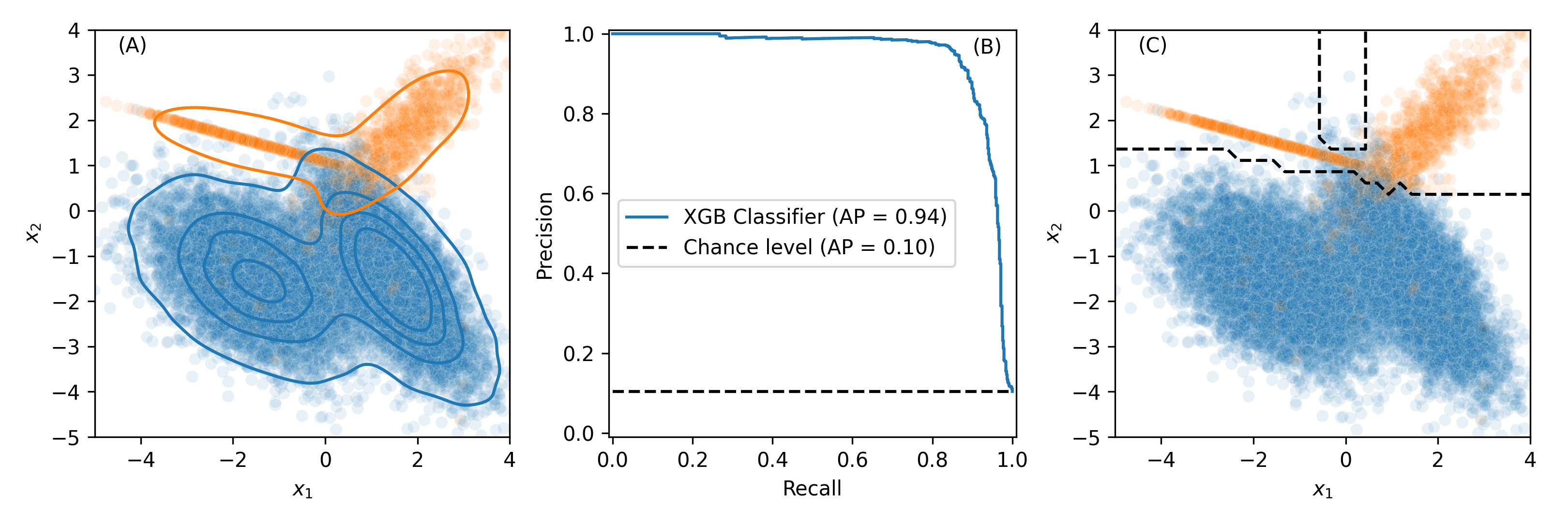
Figure 2: (A) The original classification problem with the points coloured according to their classification (orange and blue), (B) XGB classifier precision-recall curve and average precision (AP) when trained on $60\%$ of the data and tested on a $20\%$ held out fraction, and (C) the decision boundary of the classifier (dashed line).

Fig. 3 illustrates the width of the conformal prediction interval for the hypercube dataset for both LWCP and CQR. The prediction intervals are computed for an error of $\alpha=0.2$ for each conformal predictor. Additionally the more coarse grained measure of prediction set size computed from a conformal classifier is shown. These examples confirm the intuition that prediction uncertainty is larger along the decision boundary. Whilst the techniques are broadly similar, the LWCP and CQR prediction interval techniques provide a more fine-grained measurement of the local uncertainty. Note that the CQR intervals occasionally cross (denoted white in Fig. 3) - see Sec. 3.2 for details.

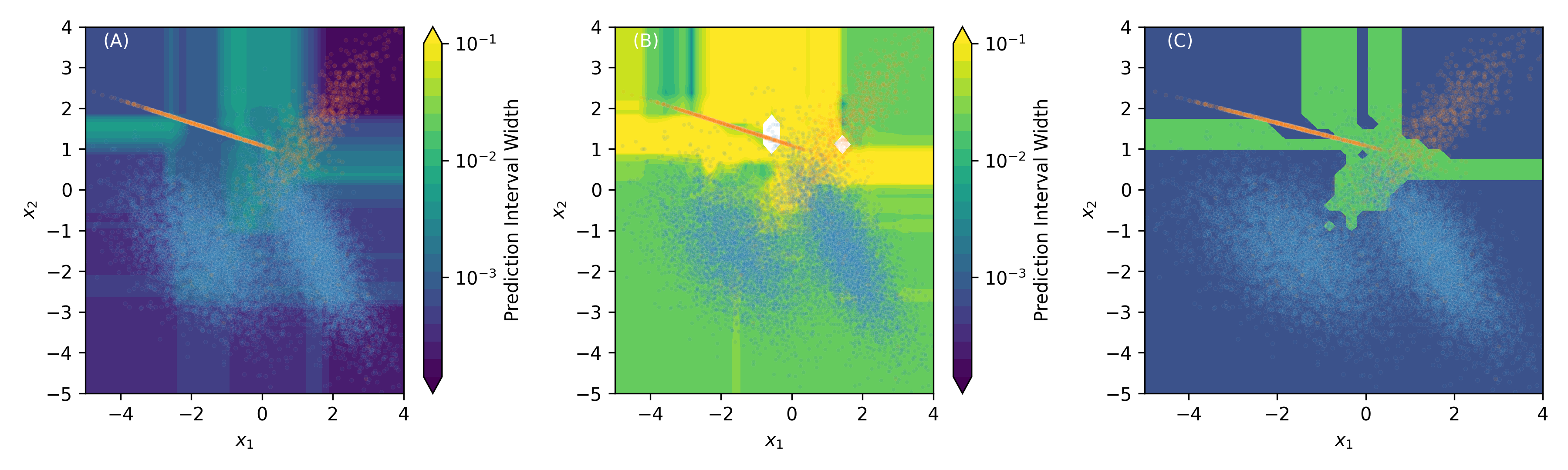
Figure 3: The prediction interval width (darker colour corresponds to smaller prediction interval) for conformal predictors with $\alpha={\color[rgb]{0,0,0}0.2}$, based on the same training set, using (A) LWCP or (B) CQR, and (C) size of the conformal prediction set based on direct binary classification The full training data $\mathcal{T}$ is overlaid (NB: white regions in (B) correspond to quantile crossing with conflicting (negative) prediction intervals).

The effect of modifying the training set on the prediction interval widths is shown in Fig. 4. Sparse datasets tend to have larger prediction intervals, particularly in regions of feature space where the minority class is present (A1). The conformal prediction interval is wider in regions where there are very few data points, as might be expected intuitively.

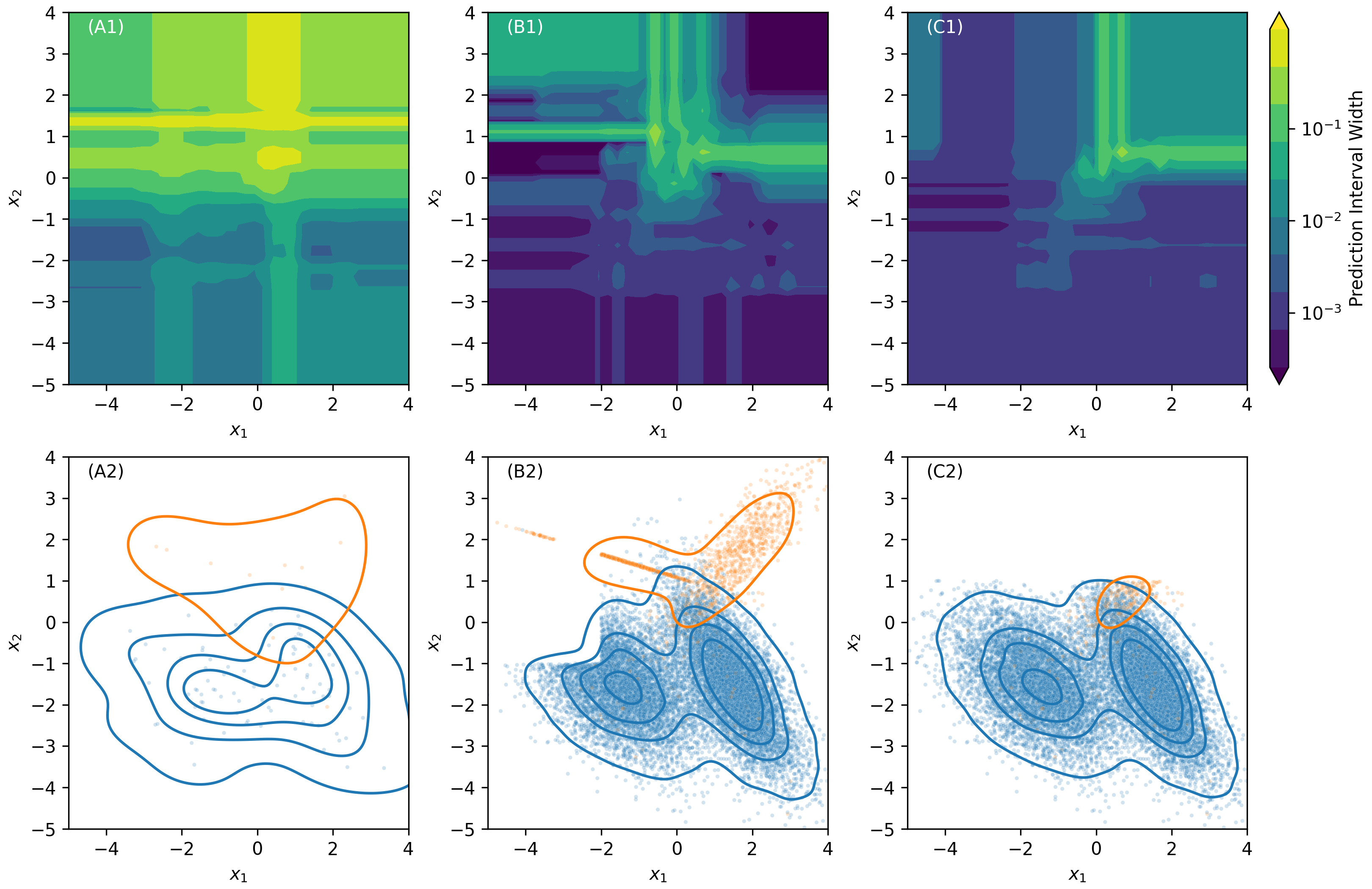
Figure 4: Prediction intervals using LWCP for different training datasets, and the same calibration data set. (A1): for the sparse training data in (A2), (B1-2): ablating an area on the left, and (C1-2): ablating all points for $x_{2}>1$.

Some CPICFs for the hypercube dataset are shown in Fig. 5. Increasing the value of $\lambda$ moves the CPICFs (white in the figure) closer to the original instance (red). This figure highlights the potential lack of diverse counterfactuals derived from this technique – if the prediction intervals have one very deep area of uncertainty, then they will tend to derive counterfactuals from this region. This might be informative for a few instances of counterfactuals, but subsequent examples will severely lack sample diversity.

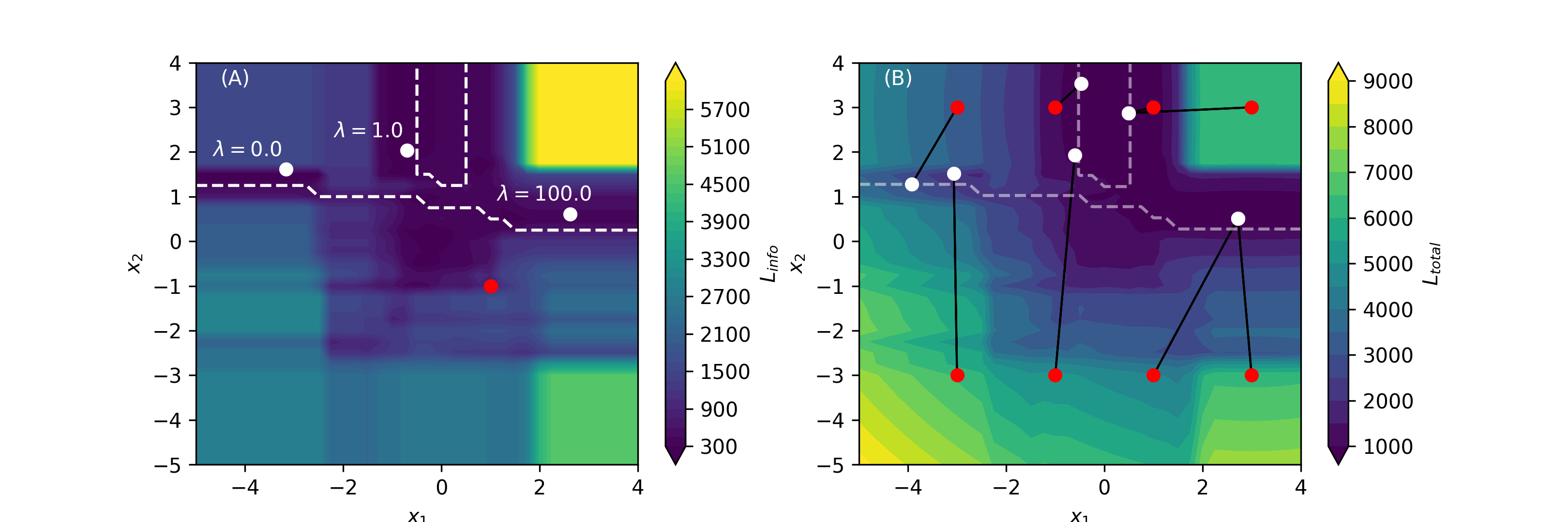
Figure 5: (A) The impact of the parameter $\lambda$ on the counterfactual selection, showing counterfactual instances for different $\lambda$ values on the $L_{\textrm{info}}$ objective function and (B) CPICFs for different starting instances for the same $L_{\textrm{total}}$ objective function.

4.1.1 Change in local prediction probability

The evaluation framework from Sec. 3.6 which measures the improvement in an individuals knowledge with a single counterfactual was applied to the hypercube dataset. We randomly selected a data subset containing $100$ sample points to represent the individual’s knowledge ${\mathcal{T}^{(k)}}$, and then generated $100$ independent CPICFs, each based on a randomly selected training point as the query instance, using sampling with replacement, with different genetic algorithm seeds, but with the same starting classifier $h_{\theta_{k}}$ to compute the conformal prediction intervals. This is repeated for $7$ independent realisations (random seeds) of the data set. Counterfactuals were generated with different objective function parameter $\lambda$, as well as with a constant objective function, chosen to select a random counterfactual. The entry “Gower distance” refers to $\lambda=10^{5}$.

Fig. 6 shows $\Delta(X)$ from (9) for $\Omega{\color[rgb]{0,0,0}(X)}$ a square of side $0.1,0.5$ and $1.0$. For $\lambda=1$ or $100$, prediction probabilities for the classifier with single additional counterfactual in the training data typically move closer to those oracle classifier $p_{\theta}$; the fraction of negative $\Delta$ is substantially larger than $50\%$. Moreover, creating counterfactuals only based on the width of the conformal prediction set ($\lambda=0$), or mainly based on the Gower distance (a large value of $\lambda=10^{5}$), or only based on being a counterfactual (“unconstrained”) on average does not improve the prediction. We also note that the size of $\Omega(X)$ does not seem to have much of an effect. Results for $\alpha=0.2$ are included in Appendix B, with a similar finding, except that the choice of $\lambda$ would then be 10. Investigating possible relationships between $\alpha$ and the best $\lambda$ will be part of future work.

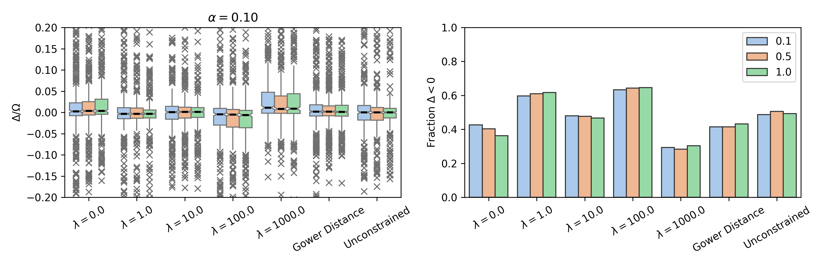
Figure 6: A boxplot (left) of the change in the MAD prediction probabilities between with and without the counterfactual in the training set. $100$ observations are sampled without replacement in equal proportion from each class in the training data. Each point corresponds to the $\Delta{\color[rgb]{0,0,0}(X)}$ following an $X^{\prime}$ obtained from $X$ in the training data. The $\Omega{\color[rgb]{0,0,0}(X)}$ used for averaging is a square around $X$ of side length $0.1$, $0.5$ and $1.0$ represented by blue, orange and green bars respectively, and the error is $\alpha=0.1$. The fraction of the $\Delta<0$ is shown on the right, illustrating that for $\lambda=1$ and $\lambda{\color[rgb]{0,0,0}=100}$ there is an improvement over using only the length of the conformal prediction interval ($\lambda=0$), or using (mainly) Gower distance ($\lambda=10^{5}$), or using general counterfactuals (“unconstrained”).

4.1.2 The effect of conformal prediction interval counterfactuals

To further assess whether CPICFs are informative, rather than considering the impact of a single counterfactual, each training data point was augmented with $0,1$ or $4$ of counterfactuals in a batch , using $\alpha=0.1$, and then the performance of an XGB classification model was evaluated on the test set. The results of these calculations on the hypercube dataset are shown in Table 1.

Sample Points	Aug. per sample	Average Precision	F1 Score	ROC AUC
50	0	$0.79\pm 0.05$	$0.76\pm 0.14$	$0.96\pm 0.01$
50	1	$0.88\pm 0.01$	$0.85\pm 0.02$	$0.96\pm 0.01$
50	4	$0.86\pm 0.04$	$0.83\pm 0.01$	$0.96\pm 0.01$
500	0	$0.87\pm 0.01$	$0.87\pm 0.01$	$0.96\pm 0.002$
500	1	$0.92\pm 0.01$	$0.90\pm 0.01$	$0.97\pm 0.001$
500	4	$0.91\pm 0.01$	$0.90\pm 0.01$	$0.97\pm 0.001$

Table 1: The performance of a classifier trained with increasing levels of data augmentation from counterfactual examples derived with $\lambda=1000$. The classifier trained on $18000$ data points achieved an average precision of $0.94$, an F1 score of $0.90$, and a ROC AUC of $0.98$. The error estimates are based on $3$ replicates.

For a small number of data points the counterfactual augmentation improve both the average precision and the F1 score, demonstrating that the counterfactual convey information to their recipient. The effectiveness of the augmentations diminished as the number of augmentations increases, potentially indicating a lack of diversity in the batch of counterfactuals. A classifier with a larger number (500) of training points improves its average precision and F1 score to a lesser degree; this model was already close to the performance ceiling of a model trained on a much larger data set.

4.2 A Transaction Fraud Dataset

Tabformer (Padhi et al., 2021) is a synthetic multivariate tabular time series transaction fraud dataset. It has $24$ million transactions from $20,000$ users, with $12$ features and a binary label isFraud? classifying each transaction. It contains continuous features such as Amount, categorical features such as Use Chip, and other categorical features with a high cardinality such as Merchant City. Tabformer has many of the characteristics that make detecting transaction fraud challenging, including a class imbalance with $<1\%$ fraudulent transactions. The dataset exhibits distributional shift, for example as new card types become available, or transaction habits change from chip and pin to online transactions.

To assess the effect of conformal prediction interval counterfactuals, for this data set , a temporal split was used. A three year period from 02-04-2015 to 02-04-2018 was used for the training set. This was further divided into $75\%$ for training and cross validation, and $25\%$ for the conformal predictor calibration set. A $1$ year period after 02-04-2018 was used for the test data set.

An XGB classifier ($h_{\theta_{({\mathcal{D}})}}$) was then trained, and used to provide the targets for the LWCP. As the data set is still imbalanced (with approximately $7500$ fraud transactions out of over $5$ million) the majority class was randomly undersampled to balance the classes. The XGB model was trained with continuous representations for the Time, and Amount features, one hot encoding for low cardinality categorical features, and target encoding for the high cardinality features such as Zip. After hyperparameter tuning the resulting model had an average precision of $0.65$, ROC AUC of $0.994$ and an F1 Score of $0.11$ on the $1$ year of hold out data in the test data set.

The dispersion model for $\hat{\rho}$ from Algorithm 1, needed for the LWCP method, was trained on a smaller dataset of $4000$ samples from the training set, representing the uncertainty in the knowledge of an individual. The derived model was used for computing CPICFs, with the parameters used given in Appendix A. A typical example of a counterfactual is given in Table 2. This example shows that the modifications made to a particular query, whilst they may be informative, are not sparse in the number of features that are changed.

Orig/CPICF	Time	Amount	User	Zip	Merchant Name	Merchant City
Orig	13.17	39.63	1816	8270	-7051934310671642798	Woodbine
CPICF	10.64	1635.89	1768	99163	-264402457929754322	Piney River

Orig/CPICF	Merchant State	Card	Use Chip	MCC	Errors?	Weekday
Orig	NJ	0	Chip	5310	nan	3
CPICF	FL	3	Online	3256	Bad Zipcode	2

Table 2: An example of a non-fraudulent transaction (Orig), and a fraudulent CPICF derived from it for the Tabformer data set, with error $\alpha=0.2$ and $\lambda=10^{4}$.

The effectiveness of the CPICFs was measured by examining their effect in data augmentation (Fig. 7). Similarly as for Figure 6 we compare the performance of the CPICFs for $\lambda=0,10,1000,$ as well as unconstrained counterfactuals (random points with the alternate class). Here we take $\alpha=0.2$.

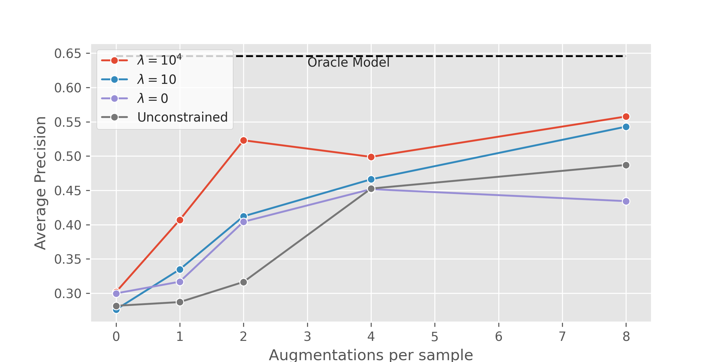
Figure 7: Average precision (area under the precision-recall curve) after training augmented with CPICF examples for the Tabformer dataset, for $\lambda\in\{0,10,10^{4}\}$, $\alpha=0.2$, and an unconstrained counterfactual with an alternate label but selected without the distance or conformal loss terms.

Adding the counterfactuals to the training set clearly improves the model performance on average, providing some evidence for the claim that CPICFs can provide a more informative augmentation when compared with unconstrained counterfactual augmentation.

5 Conclusion

Here we present a framework for a large entity (such as a bank) to derive counterfactual examples for an individual. The assumption is that the entity holds a large dataset and a potentially sensitive classifier derived from the data, while the individual has only limited knowledge of the data set. In contrast to standard approaches in counterfactual generation which use a parametric estimator of the underlying distribution, and in contrast to standard classification methods which learn a classification boundary, to compute these counterfactuals, a (nonparametric) conformal prediction set is used to express the uncertainty of the individual, who has a smaller dataset, and a less clear understanding of the decision boundary. An objective function with two terms, expressing the proximity of the counterfactual example and the uncertainty of the individual with a relative weight factor $\lambda$, is minimised, subject to the constraint of the counterfactual having the opposite classification. We call the point that achieves this minimum a conformal prediction interval counterfactual (CPICF).

This counterfactual generation method is evaluated by assessing the change in the predictive probabilities of the classification model of the individual after adding the counterfactual to the data set, and by assessing its potential for data augmentation through considering the average precision, F1 score, and ROC AUC. In our synthetic hypercube example as well as in the Tabformer data set, CPICFs can improve the prediction given an appropriate choice of the parameter $\lambda$ which trades off the importance of the distance the counterfactual is from the original point and the level of classifier uncertainty.

While our experiments validate the CPICF approach, for a practical deployment there are more experiments which could be interesting to carry out, such as whether there is a variation of the CPICF performance in different regions of the feature space. More parameter settings could be studied, and comparisons with more counterfactual generation methods could be carried out. Moreover, assessing faithfulness or fidelity, or other utility measures often employed for assessing counterfactuals, could be of interest.

Next we point out several possible improvements to the algorithm. Typically, conformal prediction techniques are model agnostic, but are data inefficient, as they require an additional data partition for the calibration set. Stutz et al. (2022) have developed a more efficient end-to-end training procedure that incorporates the calibration set during model training. Incorporation of this procedure could be linked to our pipeline as future work. Moreover, we limited ourselves to locally weighted conformal prediction techniques to compute a positive size of the interval width, as conformal quantile regression can result in quantile crossing when each quantile is fitted independently. Concurrent quantile regression models Cannon (2018) might be used to obtain non-crossing quantile models which could be explored as part of future work.

Another line of future research relates to the theoretical underpinning of the CPICF generation. Standard conformal prediction requires the input data to be exchangeable. Thus, once the counterfactual is added, the conformal prediction guarantees no longer hold. However, the CPICFs $X^{\prime}=X^{\prime}(X)$ are generated in a particular way based on prediction intervals which use the calibration data. While the CPICFs and the calibration data are not exchangeable, it may be possible to apply ideas from Hore and Barber (2025) to randomise the intervals in order to obtain theoretical guarantees; investigating this will be part of future work.

Finally, as a different application, the quantification of model uncertainty by conformal prediction interval width might be useful in contexts where the challenge is to optimise the collection of data. For example, classification probabilities to quantify the information content of an observation is often used in optimising the collection of sensor information (Krajnik et al., 2015), such as building in occupancy models from sequential collections. However this prioritisation can lead to focusing on observations that are intrinsically difficult to predict (such as occupancy during a time of transition which will always be close to $0.5$, or more generally observations at a boundary), rather than where model uncertainty could be reduced. Quantifying the uncertainty through a conformal prediction interval might lead to better sensor deployment.

The authors acknowledge the support of the UKRI Prosperity Partnership Scheme (FAIR) under EPSRC Grant EP/V056883/1 and the Alan Turing Institute, and the Bill & Melinda Gates Foundation. GR is also funded in part by the UKRI EPSRC grants EP/T018445/1, EP/X002195/1 and EP/Y028872/1.

Appendix A Model parameters

XGB hyperparameter tuning was conducted using cross validation with the following values:

Name	Values	Name	Values
n_estimators	$[80,100,120,150,300]$	max_depth	$[8,9,10,11,12]$
learning_rate	$[0.01,0.05,0.1,0.20]$	min_child_weight	$[1,2,3,4,5]$
subsample	$[0.6,0.8,1.0]$	colsample_bytree	$[0.6,0.8,1.0]$

Appendix B Supplementary Counterfactual Assessment Figures

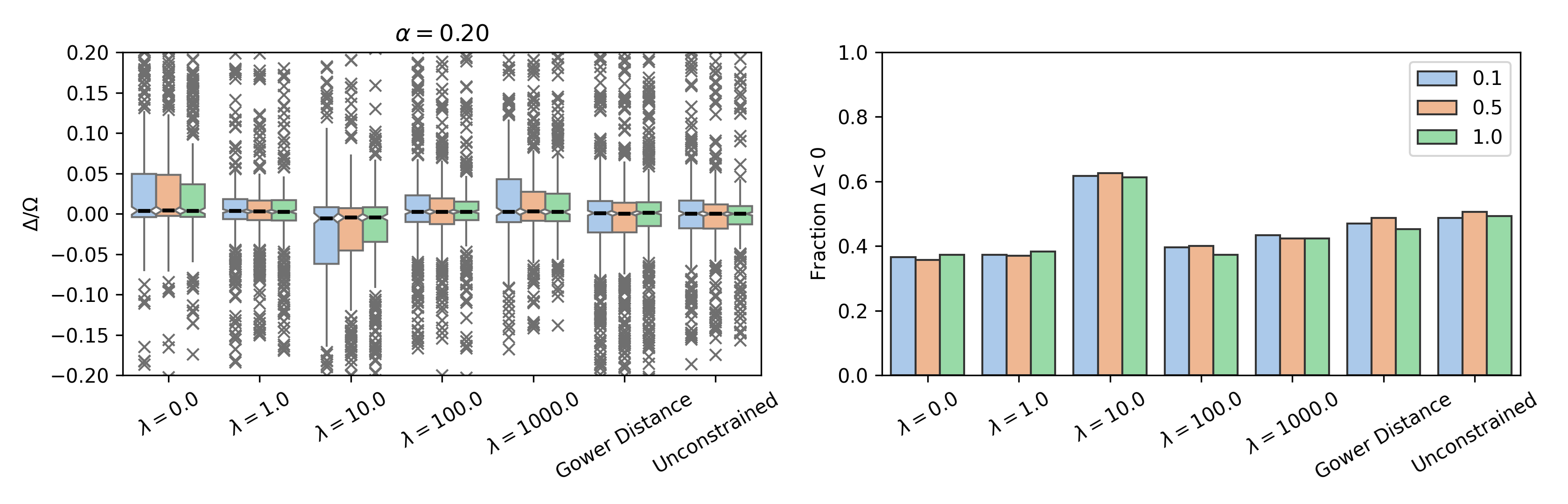
Figure 8: The change in the local model prediction following the inclusion of a counterfactual in the training set for $100$ repetitions and $7$ independent realisations of the hypercube data set, with an error of $\alpha=0.2$

While Figure 6 showed results for $\alpha=0.1$, Figure 8 shows results for $\alpha=0.2$ and illustrates that there is a regime for $\lambda$ in which there is an improvement over using mainly Gower distance ($\lambda=10^{5}$) or only the length of the conformal prediction interval ($\lambda=0$). However, now the improvement is seen for a smaller value of $\lambda$ than for $\alpha=0.1$, highlighting the need for careful calibration of $\lambda$.

References

- Altmeyer et al. (2024) Patrick Altmeyer, Mojtaba Farmanbar, Arie van Deursen, and Cynthia CS Liem. Faithful model explanations through energy-constrained conformal counterfactuals. In Proceedings of the AAAI Conference on Artificial Intelligence, volume 38, pages 10829–10837, 2024.
- Antoran et al. (2021) Javier Antoran, Umang Bhatt, Tameem Adel, Adrian Weller, and José Miguel Hernández-Lobato. Getting a CLUE: A method for explaining uncertainty estimates. In International Conference on Learning Representations, 2021.
- Blank and Deb (2020) Julian Blank and Kalyanmoy Deb. Pymoo: Multi-Objective Optimization in Python. IEEE Access, 8:89497–89509, 2020.
- Cannon (2018) Alex J. Cannon. Non-crossing nonlinear regression quantiles by monotone composite quantile regression neural network, with application to rainfall extremes. Stochastic Environmental Research and Risk Assessment, 32(11):3207–3225, 2018.
- Chen and Guestrin (2016) Tianqi Chen and Carlos Guestrin. XGBoost: A scalable tree boosting system. In Proceedings of the 22nd ACM SIGKDD International Conference on Knowledge Discovery and Data Mining, pages 785–794, 2016.
- Chen et al. (2024) Zonghao Chen, Ruocheng Guo, Jean-François Ton, and Yang Liu. Conformal counterfactual inference under hidden confounding. In Proceedings of the 30th ACM SIGKDD Conference on Knowledge Discovery and Data Mining, pages 397–408, 2024.
- Chung et al. (2021) Youngseog Chung, Willie Neiswanger, Ian Char, and Jeff Schneider. Beyond pinball loss: Quantile methods for calibrated uncertainty quantification. Advances in Neural Information Processing Systems, 34:10971–10984, 2021.
- Gammerman et al. (1998) Alex Gammerman, Volodya Vovk, and Vladimir Vapnik. Learning by transduction. In 14th Conference on Uncertainty in Artificial Intelligence, 1998.
- Goodman and Flaxman (2017) Bryce Goodman and Seth Flaxman. European Union regulations on algorithmic decision-making and a “right to explanation”. AI Magazine, 38(3):50–57, 2017.
- Guidotti (2024) Riccardo Guidotti. Counterfactual explanations and how to find them: literature review and benchmarking. Data Mining and Knowledge Discovery, 38(5):2770–2824, Sept. 2024.
- Guyon (2003) Isabelle Guyon. Design of experiments for the NIPS 2003 variable selection benchmark. NIPS, 2003.
- Hore and Barber (2025) Rohan Hore and Rina Foygel Barber. Conformal prediction with local weights: randomization enables robust guarantees. Journal of the Royal Statistical Society Series B: Statistical Methodology, 87(2):549–578, 2025.
- Krajnik et al. (2015) Tomas Krajnik, Joao M. Santos, and Tom Duckett. Life-long spatio-temporal exploration of dynamic environments. In 2015 European Conference on Mobile Robots (ECMR), pages 1–8, Lincoln, United Kingdom, Sept. 2015. IEEE.
- La Gatta et al. (2021) Valerio La Gatta, Vincenzo Moscato, Marco Postiglione, and Giancarlo Sperlì. Castle: Cluster-aided space transformation for local explanations. Expert Systems with Applications, 179:115045, 2021.
- La Gatta et al. (2025) Valerio La Gatta, Marco Postiglione, and Giancarlo Sperlì. A novel augmentation strategy for credit scoring modeling. Neural Computing and Applications, pages 1–13, 2025.
- Lei et al. (2018) Jing Lei, Max G’Sell, Alessandro Rinaldo, Ryan J. Tibshirani, and Larry Wasserman. Distribution-Free Predictive Inference for Regression. Journal of the American Statistical Association, 113(523):1094–1111, 2018.
- Lei and Candès (2021) Lihua Lei and Emmanuel J Candès. Conformal inference of counterfactuals and individual treatment effects. Journal of the Royal Statistical Society: Series B (Statistical Methodology), 83(5):911–938, 2021.
- Mendil et al. (2023) Mouhcine Mendil, Luca Mossina, and David Vigouroux. PUNCC: a Python Library for Predictive Uncertainty Calibration and Conformalization. Proceedings of Machine Learning Research, 204:1–20, 2023.
- Mohammed et al. (2022) Azhar Mohammed, Dang Nguyen, Bao Duong, and Thin Nguyen. Efficient classification with counterfactual reasoning and active learning. In Asian Conference on Intelligent Information and Database Systems, pages 27–38. 2022.
- Moreno-Barea et al. (2020) Francisco J Moreno-Barea, José M Jerez, and Leonardo Franco. Improving classification accuracy using data augmentation on small data sets. Expert Systems with Applications, 161:113696, 2020.
- Mothilal et al. (2020) Ramaravind Kommiya Mothilal, Amit Sharma, and Chenhao Tan. Explaining Machine Learning classifiers through diverse counterfactual explanations. In Proceedings of the 2020 Conference on Fairness, Accountability, and Transparency, pages 607–617, 2020.
- Padhi et al. (2021) Inkit Padhi, Yair Schiff, Igor Melnyk, Mattia Rigotti, Youssef Mroueh, Pierre Dognin, Jerret Ross, Ravi Nair, and Erik Altman. Tabular transformers for modeling multivariate time series. In IEEE International Conference on Acoustics, Speech, and Signal Processing. Institute of Electrical and Electronics Engineers Inc., 2021.
- Papadopoulos et al. (2008) Harris Papadopoulos, Alex Gammerman, and Volodya Vovk. Normalized nonconformity measures for regression Conformal Prediction. AIA ’08: Proceedings of 26th IASTED International Conference on Artificial Intelligence and Applications, pages 64–69, 2008.
- Pedregosa et al. (2011) Fabian Pedregosa, Gaël Varoquaux, Alexandre Gramfort, Vincent Michel, Bertrand Thirion, Olivier Grisel, Mathieu Blondel, Peter Prettenhofer, Ron Weiss, Vincent Dubourg, et al. Scikit-learn: Machine learning in python. Journal of Machine Learning Research, 12:2825–2830, 2011.
- Pitis et al. (2022) Silviu Pitis, Elliot Creager, Ajay Mandlekar, and Animesh Garg. Mocoda: Model-based counterfactual data augmentation. Advances in Neural Information Processing Systems, 35:18143–18156, 2022.
- Romano et al. (2019) Yaniv Romano, Evan Patterson, and Emmanuel Candes. Conformalized quantile regression. Advances in Neural Information Processing Systems, 32, 2019.
- Russell et al. (2020) Chris Russell, Rory Mc Grath, and Luca Costabello. Learning Relevant Explanations. Retrieved from https://www.researchgate.net, 2020.
- Samoilescu et al. (2021) Robert-Florian Samoilescu, Arnaud Van Looveren, and Janis Klaise. Model-agnostic and scalable counterfactual explanations via reinforcement learning. arXiv preprint arXiv:2106.02597, 2021.
- Stutz et al. (2022) David Stutz, Krishnamurthy Dj Dvijotham, Ali Taylan Cemgil, and Arnaud Doucet. Learning optimal conformal classifiers. In International Conference on Learning Representations, 2022.
- Temraz and Keane (2022) Mohammed Temraz and Mark T Keane. Solving the class imbalance problem using a counterfactual method for data augmentation. Machine Learning with Applications, 9:100375, 2022.
- Veitch et al. (2021) Victor Veitch, Alexander D’Amour, Steve Yadlowsky, and Jacob Eisenstein. Counterfactual invariance to spurious correlations: why and how to pass stress tests. In Proceedings of the 35th International Conference on Neural Information Processing Systems, pages 16196–16208, 2021.
- Verma et al. (2024) Sahil Verma, Varich Boonsanong, Minh Hoang, Keegan Hines, John Dickerson, and Chirag Shah. Counterfactual Explanations and Algorithmic Recourses for Machine Learning: A Review. ACM Computing Surveys, 56(12):1–42, Dec. 2024.
- Vivek et al. (2024) Yelleti Vivek, Vadlamani Ravi, Abhay Mane, and Laveti Ramesh Naidu. Explainable Artificial Intelligence and Causal Inference Based ATM Fraud Detection. In 2024 IEEE Symposium on Computational Intelligence for Financial Engineering and Economics (CIFEr), pages 1–7, Hoboken, NJ, USA, 2024. IEEE.
- Wachter et al. (2017) Sandra Wachter, Brent Mittelstadt, and Chris Russell. Counterfactual explanations without opening the black box: Automated decisions and the GDPR. Harvard Journal of Law & Technology, 31(2):2018, 2017.
- Wang et al. (2024) Zaitian Wang, Pengfei Wang, Kunpeng Liu, Pengyang Wang, Yanjie Fu, Chang-Tien Lu, Charu C Aggarwal, Jian Pei, and Yuanchun Zhou. A comprehensive survey on data augmentation. arXiv preprint arXiv:2405.09591, 2024.