UP-SLAM: Adaptively Structured Gaussian SLAM with Uncertainty Prediction in Dynamic Environments

Abstract

Recent 3D Gaussian Splatting (3DGS) techniques for Visual Simultaneous Localization and Mapping (SLAM) have significantly progressed in tracking and high-fidelity mapping. However, their sequential optimization framework and sensitivity to dynamic objects limit real-time performance and robustness in real-world scenarios. We present UP-SLAM, a real-time RGB-D SLAM system for dynamic environments that decouples tracking and mapping through a parallelized framework. A probabilistic octree is employed to manage Gaussian primitives adaptively, enabling efficient initialization and pruning without hand-crafted thresholds. To robustly filter dynamic regions during tracking, we propose a training-free uncertainty estimator that fuses multi-modal residuals to estimate per-pixel motion uncertainty, achieving open-set dynamic object handling without reliance on semantic labels. Furthermore, a temporal encoder is designed to enhance rendering quality. Concurrently, low-dimensional features are efficiently transformed via a shallow multilayer perceptron to construct DINO features, which are then employed to enrich the Gaussian field and improve the robustness of uncertainty prediction. Extensive experiments on multiple challenging datasets suggest that UP-SLAM outperforms state-of-the-art methods in both localization accuracy (by 59.8%) and rendering quality (by 4.57 dB PSNR), while maintaining real-time performance and producing reusable, artifact-free static maps in dynamic environments. The project: https://aczheng-cai.github.io/up_slam.github.io/

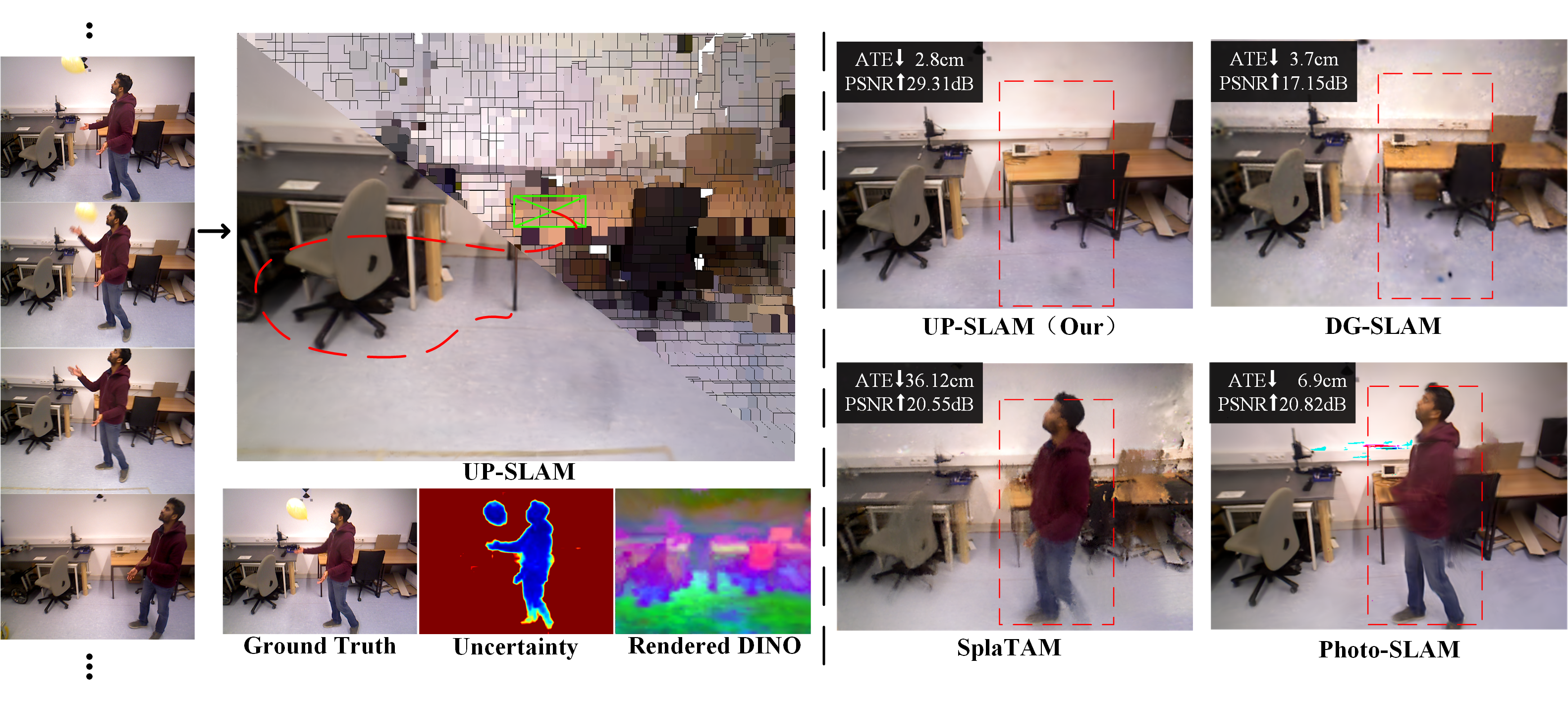
Figure 1: UP-SLAM compresses the 3DGS 3dgs representation into adaptive voxel, and constructs an artifact-free static feature map by leveraging uncertainty prediction to filter out transient objects. The dashed region on the right presents results from baseline methods. In contrast, our approach achieves high-fidelity static scene reconstructions in the presence of dynamic elements.

1 Introduction

Visual Simultaneous Localization and Mapping (SLAM) is a core technology for embodied intelligence and virtual reality. Traditional SLAM algorithms typically assume static environments, which has facilitated the development of numerous effective systems orbslam3 ; dso ; plslam . However, this assumption restricts the applicability of SLAM in dynamic real-world environments, thereby impeding advancements in robotics and related fields. Recent SLAM approaches dynaslam ; rldslam ; dsslam leverage object detection and multiple-view geometry theory to reduce the impact of dynamic objects. While these approaches enhance system robustness in dynamic environments, they heavily depend on prior knowledge of dynamic objects and the reliability of detection algorithms.

Advances in high-fidelity scene representations, such as Neural Radiance Fields nerf (NeRF) and 3D Gaussian Splatting 3dgs (3DGS), have motivated interest in introducing uncertainty modeling into 3D reconstruction. Recent studies nerfonthego ; wildgaussians ; t3dgs show that incorporating uncertainty prediction can significantly enhance robustness to transient scene elements. These uncertainty-aware models can achieve high-quality reconstructions even under intermittent occlusions. However, these methods depend on advantageous conditions, such as accurate camera poses and sparse viewpoints, which are challenging to achieve in SLAM systems using continuous frame inputs.

To address these challenges, a real-time RGB-D SLAM system named UP-SLAM is presented for robust pose estimation and static scene reconstruction in dynamic environments. Our approach compresses 3DGS into structured anchors encoded by multiple shallow multilayer perceptrons (MLPs). A probabilistic octree is introduced to enable adaptive adjustment of anchors to delete redundant anchors caused by dynamic objects. Furthermore, by decoupling motion mask generation from map optimization, UP-SLAM enables parallel tracking and mapping, supporting real-time localization. In the tracking process, we propose a training-free, optimization-based multi-modal consistency estimation method that fuses geometric cues with DINO features for effective dynamic object recognition. In the mapping process, to further enhance reconstruction under dynamic conditions, a temporal encoder that leverages sinusoidal positional encoding is designed to embed inter-frame information into the MLP, thereby increasing the representational capacity. In addition, the inconsistent appearance and motion of dynamic objects across frames provide valuable cues for uncertainty prediction. Therefore, robust DINO features are fed into a shallow MLP for per-pixel uncertainty estimation, enabling continuous motion mask refinement and enhancing reconstruction robustness.

Our primary contributions are as follows: (i) An uncertainty-aware parallel tracking and mapping framework is proposed to effectively mitigate dynamic disturbances without relying on predefined semantic annotations, thereby enabling the construction of high-quality, artifact-free static maps. (ii) We propose an adaptive structured 3DGS scene representation with a probabilistic octree, which supports automatic Gaussian primitive allocation or pruning in dynamic environments. This approach enhances localization accuracy and reduces model size. (iii) We integrate our approach into ORB-SLAM3 orbslam3 and perform comprehensive evaluations on multiple datasets. Additionally, we introduce a protocol for assessing rendering quality in dynamic environments, and we will release our datasets to the public.

2 Related work

2.1 Traditional Visual SLAM

Over the past few decades, visual SLAM has made remarkable progress, leading to the development of numerous outstanding algorithms dso ; orbslam3 ; plslam . However, these methods generally assume a static environment and neglect the velocity components in observations, making them susceptible to severe drift when dynamic objects are present. To address this issue, dynamic SLAM methods yoloslam ; dsslam based on object detection or semantic segmentation have been proposed. DynaSLAM dynaslam leverages predefined semantic labels from Mask R-CNN maskrcnn , combined with geometric constraints, to reduce the influence of dynamic objects. However, this dependence on prior labels significantly limits the generalizability of the method. To reduce reliance on semantic priors, the method pcslam takes advantage of spatial correlations between 3D points to eliminate dynamic features, while other methods spwslam ; cprslam detect inconsistencies between point clouds to localize moving objects. Most existing methods emphasize tracking robustness but neglect the construction of semantically enriched and reusable maps, which are critical for high-level tasks such as navigation and scene understanding. To bridge this gap, we design to efficiently distill high-dimensional visual features from DINOv2 dinov2 into the 3DGS representation, enabling the construction of a dense, feature-rich map that serves as a reliable foundation for downstream robotic tasks.

2.2 NeRF and 3DGS SLAM

NeRF SLAM.

Neural implicit SLAM methods have recently attracted increasing attention for their capability to reconstruct high-fidelity scenes with continuous representations. iMAPimap is the first to introduce volumetric NeRF scene representations into SLAM, encoding geometry through a single MLP and feature grid for implicit mapping. However, the long-term localization performance is hindered by the catastrophic forgetting issue associated with single-network representations. To address this, NICE-SLAM niceslam proposes a hierarchical grid-based feature structure, significantly improving scalability and real-time performance for large-scale scene reconstruction. Subsequent works such as Vox-Fusionvoxfusion , Co-SLAM coslam , and ESLAM eslam incorporate signed distance fields into hybrid representations, achieving notable gains in reconstruction quality and computational efficiency. While these methods demonstrate impressive performance in static scenes, they tend to degrade under dynamic conditions. More recent approaches have sought to extend NeRF-based SLAM to dynamic environments. For example, RodynSLAM rodynslam combines semantic priors and an optical flow estimator to mask dynamic regions. The method forget pre-trains a dynamic object classifier and incrementally updates it by feeding features from objects identified through residuals between the map and ground truth. This enables the system to learn new dynamic features over time. However, such approaches heavily rely on prior knowledge of object classes, making them less generalizable to real-world open-set environments that contain unknown dynamic objects.

3DGS SLAM.

Recently, the emergence of 3DGS techniques, leveraging GPU tile-based acceleration frameworks, has enabled extremely high-frequency rendering. Several 3DGS-based SLAM systems have been proposed cgslam ; gsorb ; gs3slam ; gaussianslam ; gsslam . For instance, SplaTAM splatam proposes a silhouette tracking strategy and uses geometric cues to initialize Gaussians in under-reconstructed regions. However, both methods exhibit a high degree of coupling between tracking and mapping, which limits their real-time performance and hampers deployment in robotic platforms. To address this, Photo-SLAM photoslam decouples tracking and mapping by employing the real-time ORB-SLAM3 tracking to provide camera poses for training images. It further proposes an image pyramid optimization strategy to improve reconstruction quality, ultimately achieving real-time tracking and high-quality mapping on embedded devices. Nevertheless, these methods still face challenges in dynamic environments. DG-SLAM dgslam addresses this by combining semantic segmentation with motion masks derived from spatial geometry consistency across frames, thereby removing the need for prior knowledge of object classes. Gassidy gassidy employs segmentation and a Gaussian mixture model to mask dynamic objects for robust tracking and high-quality map reconstruction. These methods obtain a fixed motion mask from the tracking, which can reduce the robustness of mapping. WildGS-SLAM wildslam represents a recent advancement in monocular dynamic SLAM, introducing an uncertainty-aware dynamic object recognition strategy to build high-quality, artifact-free maps. However, the tight coupling between tracking and mapping in these methods compromises real-time performance. In contrast, tracking and mapping are decoupled in our method to improve efficiency, and DINO features are fed into a shallow MLP to support continuous refinement of the motion mask, thereby supporting real-time tracking and artifact-free, high-quality map reconstruction in challenging dynamic environments.

3 Approach

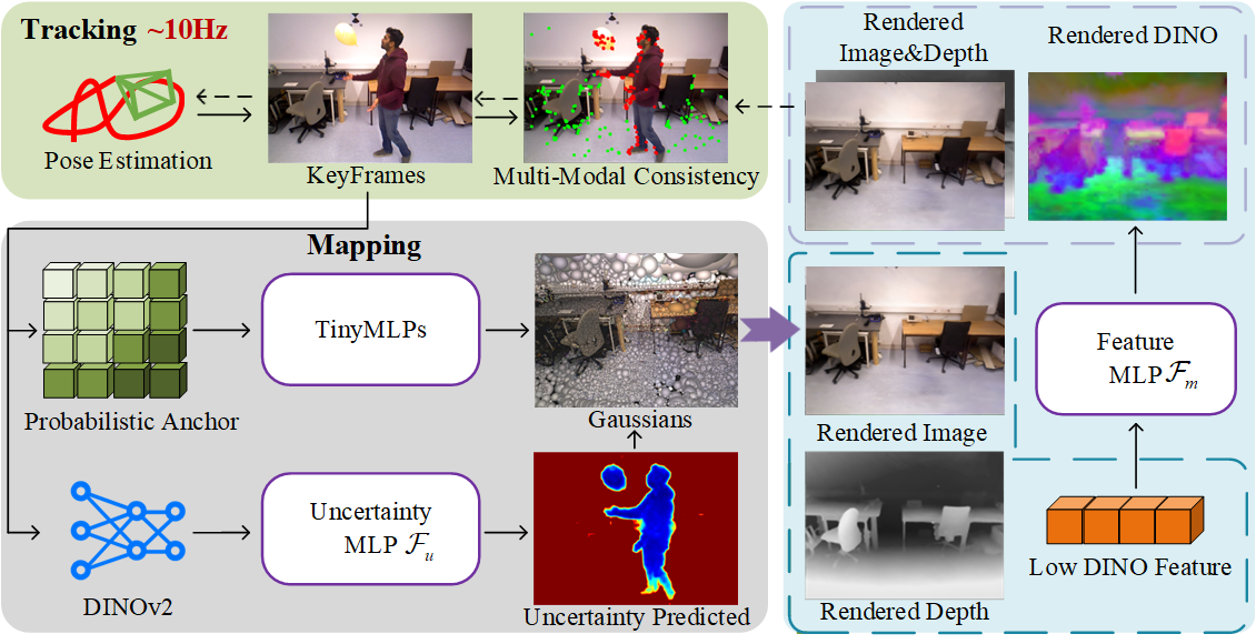
Figure 2: System overview. UP-SLAM is a parallel tracking and mapping system that enables real-time localization and high-fidelity, artifact-free map reconstruction.

An overview of the UP-SLAM system is shown in Fig. 2. UP-SLAM takes a sequence of RGB and depth images $\{\mathcal{D},\mathcal{I}\}\in\mathbb{R}^{H\times W}$ as input and adopts a parallelized tracking and mapping architecture to enhance overall efficiency. In the tracking thread (Sec. 3.4), the system performs real-time localization and generates keyframes for mapping. Dynamic region detection is guided by multi-modal residuals propagated from the mapping thread, enabling robust and real-time tracking. The mapping thread (Sec. 3.3) employs probabilistic anchors to construct an adaptively structured 3DGS representation, which reduces model size while improving reconstruction quality. To improve mapping quality in dynamic environments, robust 2D visual features extracted from DINOv2 are distilled into the 3DGS representation to construct multi-modal residuals, which supervise a shallow MLP for per-pixel uncertainty prediction and enable continuous refinement of the motion mask.

3.1 Preliminaries

Following the vanilla 3DGS 3dgs framework, the entire scene is represented by a set of anisotropic Gaussian ellipsoids G:

$${\textbf{G}}=\{{G_{i}}:(\mu_{i},o_{i},c_{i},\Sigma_{i})|i=1,...,N\},$$ (1)

where each Gaussian is defined by its color $c\in\mathbb{R}^{3}$, opacity $o\in[0,1]$, position $\mu\in\mathbb{R}^{3}$, and covariance matrix $\Sigma\in\mathbb{R}^{3\times 3}$. The covariance matrix $\Sigma$ is decomposed as $\Sigma_{i}=RS{S^{T}}{R^{T}}$, where $S$ is a scale matrix and $R$ is a rotation matrix, to ensure positive semi-definiteness.

The camera-to-world transformation $T_{wc}$ is obtained via pose estimation method, after which each 3D Gaussian point $G_{i}$ is projected onto the image plane for rendering, as follows:

$$\Sigma^{\prime}=JT_{wc}^{-1}\Sigma T_{wc}^{-T}{J^{T}},$$ (2)

where $J$ denotes the Jacobian matrix of the affine approximation to the projective function. Following the $\alpha$-blending technique, the rendered color $\tilde{C}$ and depth $\tilde{D}$ of each pixel are computed by accumulating the contributions of Gaussians along the ray. In addition, the accumulated transmittance $\tilde{T}$ is rendered to determine visibility, as formulated below:

$$\{\tilde{C},\tilde{D}\}=\sum\limits_{i=1}^{N}{\{{c_{i}},{z_{i}}\}{\sigma_{i}}}\prod\limits_{j=1}^{i-1}{(1-{\sigma_{j}})},\tilde{T}=\sum\limits_{i=1}^{N}{{\sigma_{i}}}\prod\limits_{j=1}^{i-1}{(1-{\sigma_{j}})},$$ (3)

where $c_{i}$ represents the color of the i-th 3D Gaussian, the density $\sigma_{i}$ is determined by both the Gaussian distribution function and the learned opacity $o_{i}$, the $z_{i}$ denotes the Gaussian depth value in the camera coordinate. In the optimization of Gaussian parameters, we incorporate geometric supervision as follows:

$${\mathcal{L}_{g}}=\lambda_{1}(\lambda\left\|{\tilde{C}-C}\right\|_{2}^{2}+(1-\lambda)(1-\textbf{SSIM}(\tilde{C},C)))+\lambda_{2}\left\|{\tilde{D}-D}\right\|_{2}^{2},$$ (4)

where SSIM is structural similarity index measure ssim , $\{\lambda\}$ are hyperparameters. $C$ and $D$ denote the ground-truth color and depth, respectively.

3.2 Uncertainty Model

The effectiveness of uncertainty prediction in filtering transient objects has been well demonstrated in in-the-wild 3D reconstruction tasks nerfonthego ; wildgaussians ; robustnerf . The uncertainty is modeled using a Bayesian learning framework, where the model predicts a Gaussian distribution to represent the uncertainty of each pixel, rather than outputting a single deterministic value. For each pixel, we compute the residual $R$ between the rendered value and the ground truth, with $\sigma$ denoting the predicted uncertainty. The loss for each pixel is defined as the negative log-likelihood of a normal distribution:

$${{\cal L}_{u}}=-\log(\frac{1}{{\sqrt{2\pi{\sigma^{2}}}}}\exp(-\frac{R}{{2{\sigma^{2}}}}))=\frac{R}{{2{\sigma^{2}}}}+{\lambda_{3}}\log\sigma.$$ (5)

The first term is regularized by the second term, which corresponds to the log-partition function of the normal distribution and prevents a trivial minimum at $\sigma=\infty$ nerfw .

The DINO features are inherently robust to appearance variations across frames wildgaussians , making them well-suited for dynamic scenes with inconsistent appearance features. Therefore, DINO features are incorporated into both color and depth information to achieve joint constraints across appearance, geometry, and semantics. Additionally, we employ the accumulated transmittance $\tilde{T}$ as a visibility mask to prevent low-opacity regions from contributing. The total residuals $R$ are defined as:

$$R=(\tilde{T}<0.1)(\lambda_{1}^{t}\left|{\tilde{C}-C}\right|+\lambda_{2}^{t}\left|{\tilde{D}-(D\otimes{\bf{B}})}\right|+\lambda_{3}^{t}{\left\lceil{1-\frac{{F\cdot\hat{F}}}{{{{\left\|F\right\|}_{2}}{{\left\|{\hat{F}}\right\|}_{2}}}}}\right\rceil^{1}}).$$ (6)

The B is a 3×3 box filter applied to depth via convolution ($\otimes$), and $\left\lceil{}\right\rceil^{1}$ indicates that the output is capped at 1. $F$ denotes the visual features extracted by DINOv2 dinov2 , while $\hat{F}$ signifies the rendered high-dimensional visual features. Since DINOv2 is defined per image patch, we perform bilinear interpolation to upsample it to the image size for similarity calculation.

3.3 Mapping

Adaptively Structured Gaussian.

3DGS SLAM techniques require the rapid identification of under-reconstructed regions and the initialization of new Gaussian primitives to improve tracking efficiency. Currently, many 3DGS SLAM systems rely on manually tuned thresholds to detect under-reconstructed regionsgsorb ; splatam ; gsslam . However, The threshold-dependent initialization strategies become increasingly unreliable in dynamic environments. Inappropriate threshold settings may lead to excessive GPU memory consumption, reduced computational efficiency, and even degraded rendering quality.

An incremental probabilistic anchor method is proposed to achieve adaptively structured 3DGS, eliminating the need for complex threshold tuning and manual management of Gaussian primitives. Specifically, we decode the $k$ Gaussian attributes from the anchor features ${\hat{f}}_{v}$, as well as the relative direction $\delta_{vc}$ and distance ${\vec{d}}_{vc}$ between the camera center and the anchor, using an MLP scaffold . In contrast, our anchors are equipped with probabilistic attributes, where the probability value reflects the degree of motion at each anchor. This probabilistic representation is more suitable for dynamic environments. The probabilistic anchor update equation is as follows octomap :

$$P(n|{z_{1:t}})={[1+\frac{{1-P(n|{z_{t}})}}{{P(n|{z_{t}})}}\frac{{1-P(n|{z_{1:t-1}})}}{{P(n|{z_{1:t-1}})}}\frac{{P(n)}}{{P(n)}}]^{-1}}.$$ (7)

This update equation is based on Bayes theorem and requires a prior probability $P(n)$, the current observation $z_{t}$, and the likelihood model $P(n|z_{1:t-1})$ to update the dynamic probability of each anchor. $P(n\mid z_{t})$ denotes the probability that anchor $n$ is occupied, given the observation $z_{t}$.

Temporal Encoding.

Methods such as scaffold ; wildgs introduce appearance embeddings into the color prediction to improve rendering quality in wild reconstruction. These methods are primarily designed to improve rendering quality through better representation learning. In the context of SLAM, the method scaffoldslam leverages the pose as an additional input to the MLP, utilizing the characteristics of SLAM to enhance performance. However, since the rotation matrix lies on the special orthogonal group $SO(3)$, a non-Euclidean manifold with nonlinear constraints, conventional MLPs struggle to model rotational variations effectively rotation , leading to suboptimal performance. Given that SLAM operates on temporally correlated image sequences where pose evolution is time-dependent, we propose a temporal encoding method to further enhance rendering quality. Specifically, each sequence $t$ is mapped to a temporal embedding ${\ell_{t}}=\{\sin(\pi t),\cos(\pi t)\}\in{\mathbb{R}^{2}}$, which improves the representational capacity of all MLPs. For example, the color {c} is predicted using an MLP conditioned on both spatial and temporal features:

$$\{{c_{0}},...,{c_{k-1}}\}={\mathcal{F}_{c}}({{\hat{f}}_{v}},{\delta_{vc}},{{\vec{d}}_{vc}},{\ell_{t}}).$$ (8)

Similarly, opacity $\{o\}$, rotation $\{q\}$, and scale $\{s\}$ are each predicted by their individual MLPs.

Visual Feature.

The inclusion of high-dimensional visual features significantly expands the Gaussian optimization space, leading to higher memory consumption and reduced computational efficiency. Inspired by featuregs ; gs3slam , anchor features are employed to decode low-dimensional Gaussian visual attributes $\{f\}\in\mathbb{R}^{k\times N_{l}}$ via an MLP $\mathcal{F}_{d}$:

$$\{{f_{0}},...,{f_{k-1}}\}={\mathcal{F}_{d}}({{\hat{f}}_{v}},{\delta_{vc}},{{\vec{d}}_{vc}},{\ell_{t}}),$$ (9)

Similar to color rendering, the low-dimensional features are rendered through the 3DGS framework, yielding the rendered feature representation $\tilde{F}$, as defined below:

$$\tilde{F}=\sum\limits_{i=1}^{N}{{f_{i}}{\sigma_{i}}}\prod\limits_{j=1}^{i-1}{(1-{\sigma_{j}})}.$$ (10)

To align the low-dimensional Gaussian parameters with the high-dimensional $N_{h}$ visual features, we employ a shallow MLP $\mathcal{F}_{m}$ to map them into a higher-dimensional space and obtain high-dimensional visual features $\hat{F}$:

$$\hat{F}={\mathcal{F}_{m}}({\tilde{F}})\in\mathbb{R}^{N_{h}}.$$ (11)

We supervise the learning of DINO features $F$ and rendering features $\hat{F}$ through a loss function $\mathcal{L}_{d}$:

$$\mathcal{L}_{d}=\frac{1}{N_{d}}\sum\limits_{i=0}^{N_{d}}\left(1-\frac{F_{i}\cdot\hat{F}_{i}}{\left\|F_{i}\right\|_{2}\left\|\hat{F}_{i}\right\|_{2}}\right),$$ (12)

where $N_{d}$ is the feature dimension of DINO, $i$ is the i-th vector. Since $N_{l}<<N_{h}$, visual features $\hat{F}$ are efficiently distilled into the 3DGS representation, preserving optimization efficiency while reducing memory and computational overhead.

Uncertainty Prediction for Mapping.

In traditional SLAM systems, the tracking module performs real-time localization, while the mapping module focuses on mitigating accumulated drift and optimizing the map. This paradigm is followed in our work, where the mapping process is extended to include not only the optimization of the static scene representation but also the refinement of the motion mask, thereby enhancing both robustness and reconstruction quality. Specifically, DINO features are fed into an MLP $\mathcal{F}_{u}$, which predicts per-pixel uncertainty:

$$\sigma=\mathcal{F}_{u}(F),$$ (13)

and the parameters of the MLP $\mathcal{F}_{u}$ are optimized under the supervision of the loss function $L_{u}$. The uncertainty map is then binarized to generate a motion mask $M=\delta(2{\sigma^{2}}>1)$, where $\delta$ denotes an indicator function that returns true when the condition is satisfied. To ensure multimodal consistency of G in dynamic environments, $\mathcal{L}$ encompasses constraints related to appearance, semantics, geometric and motion mask as follows:

$$\mathcal{L}={M}(\mathcal{L}_{g}+\lambda_{4}\mathcal{L}_{d})+\lambda_{5}\bar{s},$$ (14)

where $\bar{s}$ denotes the mean scale, introduced to prevent scale explosion. During each Gaussian optimization iteration, the uncertainty MLP $\mathcal{F}_{u}$ is optimized simultaneously. However, the gradient flows from the mapping loss $\mathcal{L}$ and the uncertainty loss $\mathcal{L}_{u}$ are kept separate to ensure independent parameter updates.

3.4 Tracking

Previous methods such as wildslam ; forget ; dgslam follow a sequential tracking-mapping pipeline, in which camera pose estimation is followed by scene representation optimization, and dynamic object recognition is typically performed after map convergence. However, this tight coupling between modules limits the ability to achieve real-time localization in dynamic environments.

Therefore, to achieve a parallel tracking and mapping framework, a training-free estimator is proposed to decouple motion mask generation from global scene optimization. By exploiting the fast rendering capabilities of 3DGS, multi-modal residuals $R$ are computed and fed in real time into the following objective function $\xi$, from which an uncertainty map $\sigma$ is optimized:

$$\xi(\sigma)=\mathop{\min}\frac{1}{{HW}}\sum\limits_{i=1}^{H}{\sum\limits_{j=1}^{W}{\frac{1}{2}\left({\frac{{{R_{ij}}}}{{{\sigma^{2}}}}+\log\sigma}\right)}}.$$ (15)

The uncertainty map is subsequently thresholded to generate a motion mask, which is used to filter out dynamic keypoints from the keyframes, preventing them from being converted into landmarks.

During initialization, the complete extraction of dynamic regions is essential for feature-based SLAM, as even partial inclusion of dynamic features can lead to long-term drift or tracking failure. To enhance mask completeness, we refine motion mask by computing its intersection over union with segmentation results from YOLOv8-seg yolov8 , ensuring more thorough exclusion of dynamic regions. While YOLOv8-seg is trained on a closed set of categories, our residual-guided refinement strategy allows UP-SLAM to generalize effectively to untrained dynamic objects mask, as illustrated in Fig. 3.

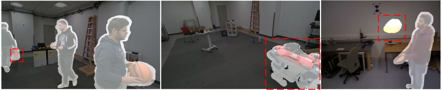
Figure 3: Open-set capability in tracking. The categories within the red box are all without pre-training, and the bright regions indicate the detected dynamic objects.

4 Experiments

Table 1: Tracking results on Bonn RGB-D dataset. (ATE RMSE$\downarrow$[cm])

Method	Balloon	Balloon2	Ball_track	Ps_track	Ps_track2	Mv_box2	Avg.
ORB-SLAM3	5.8	17.7	3.1	70.7	77.9	3.5	29.78
DynaSLAM	3.0	2.9	4.9	6.1	7.8	3.9	4.76
ESLAM	22.6	36.2	12.4	48	51.4	17.7	31.38
RoDyn-SLAM	7.9	11.5	13.3	14.5	13.8	12.6	12.26
Photo-SLAM	6.9	26	3.2	76.4	87.4	3.6	33.91
GS-SLAM	37.5	26.8	31.9	46.8	50.4	4.8	33.03
DG-SLAM	3.7	4.1	10	4.5	6.9	3.5	5.45
UP-SLAM(Our)	2.8	2.7	2.9	4.0	3.6	3.2	3.2

Table 2: Tracking results on MoCap RGB-D dataset. "X" denotes a tracking failure. (ATE RMSE$\downarrow$[cm])

Method	ANY1	ANY2	Ball	Crowd	Person	Racket	Stones	Table1	Table2	Umb.	Avg.
DynaSLAM	1.6	0.5	0.5	1.7	0.5	0.8	2.1	1.2	34.8	34.7	7.84
NICE-SLAM	X	123.6	21.1	X	150.2	X	134.4	138.4	X	23.8	-
Photo-SLAM	79.5	11.8	50.3	105.9	27.5	38.23	113.5	39.1	64.8	84	61.46
DG-SLAM	1.2	2.1	0.8	1.3	1.5	1.6	1.5	2	57.9	1.35	7.06
UP-SLAM(Our)	0.4	0.6	0.6	1.1	1.1	0.9	1.0	0.7	3.6	0.8	1.08

Table 3: Tracking results on TUM RGB-D dataset. (ATE RMSE$\downarrow$ [cm])

Method	Fr3/w/xyz	Fr3/w/half	Fr3/w/static	Fr3/s/xyz	Fr2/desk_person	Avg.
ORB-SLAM3	28.1	30.5	2.0	1.0	1.5	12.62
DynaSLAM	1.5	2.9	0.7	1.6	0.9	1.52
Co-SLAM	51.8	105.1	49.5	6	7.6	44
RoDyn-SLAM	8.3	5.6	1.7	5.1	5.6	5.26
Photo-SLAM	60.4	35.7	13.7	1.0	0.6	22.28
DG-SLAM	1.7	1.8	0.7	1.0	3.2	1.68
UP-SLAM(Our)	1.6	2.6	0.7	0.9	1.3	1.42

4.1 Experimental Setup

To demonstrate the competitiveness of our approach, we compare it against 16 methods, categorized as follows: (a) Classic SLAM methods: ORB-SLAM3 orbslam3 ; (b) Classic dynamic SLAM methods: ReFusion refusion , DynaSLAM dynaslam , EM-Fusion emfusion ; (c) NeRF-based SLAM methods: iMAP imap , NICE-SLAM niceslam , Vox-Fusion voxfusion , Co-SLAM coslam , ESLAM eslam ; (d) NeRF-based dynamic SLAM: RoDyn-SLAM rodynslam ; (e) 3DGS-based SLAM: Photo-SLAM photoslam , GS-SLAM gsslam , SplaTAM splatam ; (f) 3DGS-based dynamic SLAM methods: DG-SLAM dgslam , Gassidy gassidy , WildGS-SLAM wildslam . All methods are evaluated using dynamic datasets, specifically the TUM RGB-D Dataset tum , the Bonn RGB-D Dataset bonn , and the MoCap RGB-D Dataset wildslam , in addition to a static environment dataset, the ScanNet Dataset scannet . We report original results for non-open-source methods, and average results over five runs for open-source ones. Bold is the best result, and underline is the second best result. We select representative baselines from each category. Additional experimental results, dataset details, evaluation metrics, limitations and implementation details are provided in Appendix A.

Table 4: Ablation study on Bonn RGB-D dataset. Bold is the best result.

	ATE	PSNR	Model Size	Sim.
w/o Time.	3.37	26.6	7.04	78.6
w/o Seg.	3.46	27.1	7.03	78.5
w/o Prob.	3.57	27.74	22.92	79.2
UP-SLAM(Our)	3.2	28	7.01	79.5

Table 5: Tracking results on Scannet dataset. Bold is the best result. (ATE RMSE$\downarrow$ [cm])

Method	00	59	106	169	207	Avg.
Co-SLAM	7.1	11.1	9.4	5.9	7.1	8.8
SplaTAM	12.8	10.1	17.7	12.1	7.5	11.9
DG-SLAM	7.9	11.5	8.0	8.3	8.2	8.6
UP-SLAM(Our)	8.2	7.3	8.2	8.8	7.0	7.9

Table 6: Rendering performance comparison of SLAM methods on Bonn RGB-D dataset.

Sequence	Metric	Balloon	Balloon2	Ball_track	Ps_track	Ps_track2	movbox2	Avg.
SplaTAM	PSNR$\uparrow$	20.55	18.74	20.44	17.41	16.27	22.43	19.30
	SSIM$\uparrow$	0.829	0.756	0.819	0.438	0.625	0.881	0.724
	LPIPS$\downarrow$	0.184	0.247	0.207	0.307	0.339	0.158	0.240
Photo-SLAM	PSNR$\uparrow$	20.82	22.80	25.31	22.63	23.72	25.60	23.48
	SSIM$\uparrow$	0.814	0.830	0.833	0.803	0.814	0.859	0.825
	LPIPS$\downarrow$	0.210	0.175	0.183	0.272	0.254	0.159	0.208
DG-SLAM	PSNR$\uparrow$	17.15	16.32	16.63	18.62	17.60	18.48	17.46
	SSIM$\uparrow$	0.779	0.752	0.672	0.748	0.715	0.805	0.745
	LPIPS$\downarrow$	0.393	0.396	0.535	0.506	0.540	0.415	0.464
WildGS-SLAM(RGB)	PSNR$\uparrow$	25.02	24.24	22.33	22.93	22.82	23.25	23.43
	SSIM$\uparrow$	0.961	0.950	0.929	0.941	0.946	0.921	0.941
	LPIPS$\downarrow$	0.143	0.154	0.212	0.198	0.163	0.245	0.185
UP-SLAM(Our)	PSNR$\uparrow$	29.31	28.03	27.58	27.98	27.47	27.67	28.0
	SSIM$\uparrow$	0.921	0.919	0.886	0.899	0.896	0.903	0.904
	LPIPS$\downarrow$	0.089	0.100	0.144	0.128	0.118	0.128	0.117

Table 7: Additional experiments on Bonn balloon sequence. SplaTAM and DG-SLAM do not involve refinement, hence no extra time is spent. "-" indicates the absence of this component. Bold is the best result.

	Avg.$/$frame$\downarrow$[ms]	Total Time(+refine)$\downarrow$[s]	Model Size$\downarrow$[MB]
SplatTAM	4046	1776.54(+0)	29.9
WildGS-SLAM	1838	1526.584(+719.61)	8.8
DG-SLAM	1011	444.1684(+0)	-
UP-SLAM(Our)	78	694.814(+660.309)	4.9

4.2 Evaluation of Tracking Performance

Dynamic Scenes.

Our method achieves an average improvement of 59.8% in localization accuracy compared to DG-SLAM. Notably, as shown in Table 2, it improves average localization accuracy by 84.7%, primarily because DG-SLAM achieves open-set capability based on historical geometric information, which is less robust in complex dynamic environments. While DynaSLAM performs well in Table 3 due to its predefined dynamic object handling strategy, it exhibits noticeable drift in Tables 1,2. This degradation arises from the presence of numerous dynamic objects that are difficult to predefine in those datasets, especially in the Table2 and the Umbrella (Umb.) sequences.

Static Scenes.

UP-SLAM is evaluated on the public static ScanNet scannet dataset to assess robustness. While dynamic object recognition is utilized to improve the robustness of SLAM systems in dynamic environments, inaccurate recognition can adversely affect localization accuracy in static scenes. As shown in Table 5, our approach achieves an average improvement of 10.2% in localization accuracy over SLAM systems designed for static environments. Moreover, it achieves an 8.1% improvement on average compared to DG-SLAM, which is also designed for dynamic scenes. These results demonstrate that our approach maintains strong performance in both static and dynamic environments.

4.3 Evaluation of Mapping Performance

As reported in Table 6, our method achieves a notable improvement in rendering quality, with an average increase of 5.47 dB in PSNR. Photo-SLAM achieves rendering quality comparable to WildGS-SLAM, primarily due to its robustness in low-dynamic sequences (e.g., Ball_track and Mv_box2). However, in highly dynamic environments, localization failures diminish the practical significance of the rendering results. Additionally, the absence of a robust Gaussian primitive initialization strategy in DG-SLAM leads to incomplete reconstructions, significantly degrading rendering quality. Fig. 4 provides a visual comparison of the rendered results. The two static SLAM methods, SplaTAM and Photo-SLAM, fail to generate a static map. Both DG-SLAM and the monocular dynamic SLAM method WildGS-SLAM exhibit varying degrees of failure. In contrast, UP-SLAM effectively removes dynamic objects and constructs a high-fidelity, artifact-free static map.

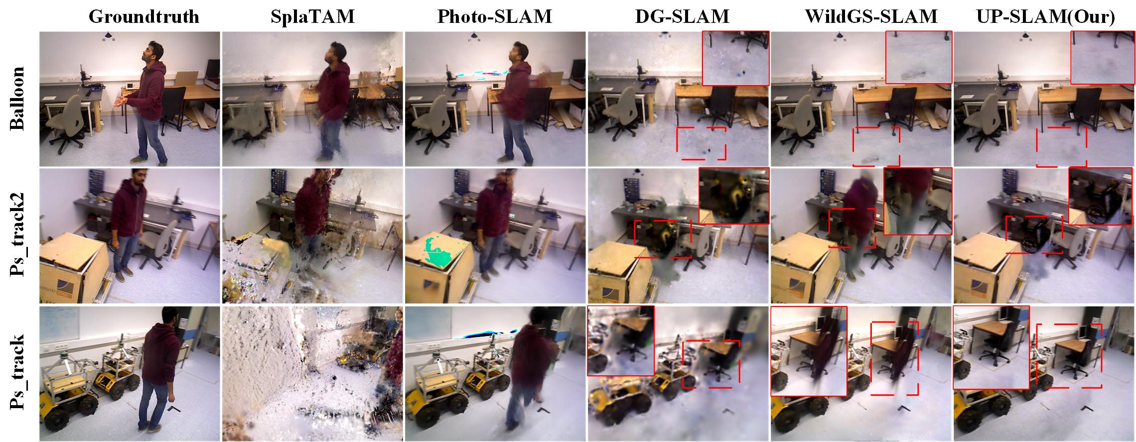
Figure 4: The rendering visualization results on Bonn RGB-D dataset. The red box is a zoom-in of the red dashed box.

4.4 Ablation Study

Localization accuracy ($\downarrow$[cm]), rendering PSNR ($\uparrow$[dB]), model size ($\downarrow$[MB]), and DINO feature similarity (Sim. $\uparrow$[%]) are quantified to comprehensively evaluate the contribution of each component, as summarized in Table 5. The temporal encoding primarily enhances rendering quality, yielding an average PSNR improvement of 1.4 dB. The segmentation module proves critical for both localization and rendering. In the initialization phase, the presence of non-rigid objects hinders segmentation of entire dynamic regions, causing potentially dynamic keypoints to be incorrectly added as static ones to the map, where they are then used as landmarks for localization. The probabilistic anchor update module significantly reduces model size, improving its suitability for deployment on embedded platforms. Without anchor updates, Gaussian primitives cannot be effectively pruned, leading to slower map updates and weakened residual feedback to the tracking thread, ultimately degrading pose estimation accuracy. Moreover, UP-SLAM improves similarity scores to nearly 80%, demonstrating its potential for downstream applications such as object-level navigation and semantic understanding.

4.5 Runtime Analysis

Table 7 presents the runtime analysis. By decoupling motion mask generation from map optimization, our system achieves a parallel tracking and mapping architecture. This enables a processing rate of 12 Hz per frame, meeting the real-time localization requirements for robotics. Compared to WildGS-SLAM, we adopt the same number of refine optimization iterations but achieve a 2× speed-up. DG-SLAM excludes segmentation time from the reported runtime. While it exhibits the fastest overall runtime, our method offers a better balance between reconstruction quality and localization speed. This trade-off is reasonable, given that mapping is typically less constrained by real-time requirements than tracking. Additionally, the use of probabilistic anchor updates and MLP-based Gaussian attribute encoding significantly reduces the overall model size.

Appendix A Technical Appendices

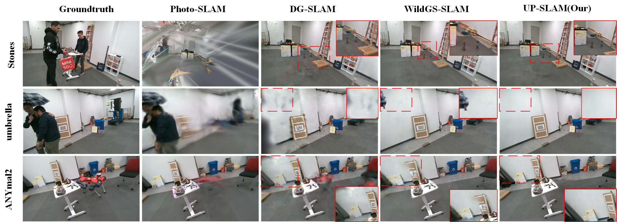
Figure 5: The rendering visualization results on MoCap RGB-D dataset. The red box is a zoom-in of the red dashed box.

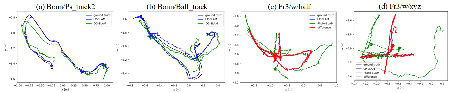
Figure 6: Localization trajectory comparisons. (a) and (b) show the trajectory comparison with DG-SLAM, while (c) and (d) compare with Photo-SLAM. The red lines indicate the deviation from the ground truth, with shorter lengths reflecting higher localization accuracy.

Dataset.

Our method is evaluated on the TUM RGB-D Dataset tum , the Bonn RGB-D Dynamic Dataset bonn , the MoCap RGB-D Dataset wildslam , and the static environment ScanNet Dataset scannet . In the TUM dataset, the primary dynamic objects are humans. In the Bonn dataset, in addition to humans, a small number of other dynamic objects, such as balloons and boxes, are present. The image resolution for both datasets is 640×480. In contrast, the MoCap RGB-D dataset features a higher image resolution of 1280×720 and contains a large number of unstructured dynamic objects beyond humans, such as robotic dogs, rocks, and other irregular entities. This poses significant challenges for dynamic SLAM methods that rely on predefined dynamic object categories. In the selected ScanNet dataset sequences, RGB-D streams with a resolution of 640×480 are captured in real indoor static environments, and the ground-truth camera poses are provided.

Baseline.

The baselines we selected are the same as those in Sec. 4.1. For better analysis, we group methods of the same category together.

Metrics.

For tracking evaluation, the official TUM evaluation script is used to jointly align the estimated and ground-truth poses and compute the RMSE of the Absolute Trajectory Error (ATE). In dynamic scenes, traditional rendering-based evaluation metrics (e.g., PSNR, SSIM, LPIPS) may become unreliable, as they are designed to assess performance under static conditions. This misalignment contrasts with our goal of reconstructing a clean static background despite the presence of dynamic elements. To address this, we adopt pre-generated dynamic object masks obtained using Ground-DINO groundingdino on the Bonn dataset. During evaluation, these masks are applied to exclude dynamic regions, ensuring that the rendering quality metrics reflect the fidelity of the static background reconstruction. Moreover, we will release the generated mask dataset to facilitate future research.

Table 8: Tracking results on Bonn RGB-D dataset (ATE RMSE$\downarrow$ [cm]). "-" indicates unavailable data because the related work is not open. Bold is the best result, and underline is the second best result.

Method	Balloon	Balloon2	Ball_track	Ps_track	Ps_track2	Mv_box2	Avg.
ORB-SLAM3	5.8	17.7	3.1	70.7	77.9	3.5	29.78
ReFusion	17.5	25.4	30.2	28.9	46.3	17.9	27.7
DynaSLAM	3	2.9	4.9	6.1	7.8	3.9	4.76
iMap	14.9	67	24.8	28.3	52.8	28.3	36.01
NICE-SLAM	X	66.8	21.2	54.9	45.3	31.9	36.68
Vox-Fusion	65.7	82.1	43.9	128.6	162.2	31.9	85.73
Co-SLAM	28.8	20.6	38.3	61	59.1	70	46.3
ESLAM	22.6	36.2	12.4	48	51.4	17.7	31.38
RoDyn-SLAM	7.9	11.5	13.3	14.5	13.8	12.6	12.26
Photo-SLAM	6.9	26	3.2	76.4	87.4	3.6	33.91
GS-SLAM	37.5	26.8	31.9	46.8	50.4	4.8	33.03
SplaTAM	36.12	35.1	12.93	128.7	136.5	20.6	61.65
DG-SLAM	3.7	4.1	10	4.5	6.9	3.5	5.45
GassiDy	2.6	7.6	-	10.3	13	5.4	7.78
UP-SLAM(Our)	2.8	2.7	2.9	4.0	3.6	3.2	3.2

Table 9: Tracking results on MoCap RGB-D dataset (ATE RMSE$\downarrow$ [cm]). "-" indicates unavailable data because the related work is not open. "X" denotes a tracking failure. Bold is the best result, and underline is the second best result.

Method	ANY1	ANY2	Ball	Crowd	Person	Racket	Stones	Table1	Table2	Umb.	Avg.
ReFusion	4.2	5.6	5	91.9	5	10.4	39.4	99.1	101	10.7	37.23
DynaSLAM	1.6	0.5	0.5	1.7	0.5	0.8	2.1	1.2	34.8	34.7	7.84
NICE-SLAM	X	123.6	21.1	X	150.2	X	134.4	138.4	X	23.8	-
Photo-SLAM	79.5	11.8	50.3	105.9	27.5	38.23	113.5	39.1	64.8	84	61.46
DG-SLAM	1.2	2.1	0.8	1.3	1.5	1.6	1.5	2	57.9	1.35	7.06
UP-SLAM(Our)	0.4	0.6	0.6	1.1	1.1	0.9	1.0	0.7	3.6	0.8	1.08

Table 10: Tracking results on TUM RGB-D dataset (ATE RMSE$\downarrow$ [cm]). "-" indicates unavailable data because the related work is not open. "X" denotes a tracking failure. Bold is the best result, and underline is the second best result.

Method	Fr3/w/xyz	Fr3/w/half	Fr3/w/static	Fr3/s/xyz	Fr2/desk_person	Avg.
ORB-SLAM3	28.1	30.5	2.0	1.0	1.5	12.62
ReFusion	9.9	10.4	1.7	4.0	-	6.5
DynaSLAM	1.5	2.9	0.7	1.6	0.9	1.52
EM-Fusion	6.6	5.1	1.4	3.7	-	4.2
iMap	111.5	X	137.3	23.6	119	97.85
NICE-SLAM	113.8	X	88.2	7.9	X	69.96
Vox-Fusion	146.6	X	109.9	3.8	X	86.76
Co-SLAM	51.8	105.1	49.5	6	7.6	44
ESLAM	45.7	60.8	93.6	7.6	X	51.92
RoDyn-SLAM	8.3	5.6	1.7	5.1	5.6	5.26
Photo-SLAM	60.4	35.7	13.7	1.0	0.6	22.28
GS-SLAM	37.2	60.0	8.4	2.7	8.6	23.38
SplaTAM	140.6	153.58	90.36	1.6	5.4	78.30
DG-SLAM	1.7	1.8	0.7	1.0	3.2	1.68
GassiDy	3.5	3.7	0.6	-	-	2.6
UP-SLAM(Our)	1.6	2.6	0.7	0.9	1.3	1.42

Table 11: Tracking results on Scannet dataset (ATE RMSE$\downarrow$ [cm]). Bold is the best result.

Method	00	59	106	169	207	Avg.
NICE-SLAM	12	14	7.9	10.9	6.2	10.7
Co-SLAM	7.1	11.1	9.4	5.9	7.1	8.8
Point-SLAM	10.2	7.8	8.7	22.2	14.8	12.2
Vox-Fusion	68.8	24.1	8.4	27.2	9.4	27.58
GS-SLAM	13.6	7.6	8.1	13.7	34.6	15.1
SplaTAM	12.8	10.1	17.7	12.1	7.5	11.9
DG-SLAM	7.9	11.5	8.0	8.3	8.2	8.6
UP-SLAM(Our)	8.2	7.3	8.2	8.8	7.0	7.9

Implementation Details.

UP-SLAM is fully implemented in C++ and CUDA, and runs on a desktop equipped with Intel i7-12700KF and an NVIDIA RTX 4060ti 16G GPU. We set the loss weight: {$\lambda$,$\lambda_{1}$,$\lambda_{2}$,$\lambda_{3}$,$\lambda_{4}$,$\lambda_{5}$}={$0.8$,$0.6$,$1.0$,$0.4$,$0.01$}, the residuals weight is {$\lambda_{1}^{t}$,$\lambda_{2}^{t}$,$\lambda_{3}^{t}$}={$0.25$,$0.7$,$0.1$}, the refinement iteration count: 20000, and low-dimensional $N_{l}=16$.

MLP Implementation Details.

The architecture of MLP $\mathcal{F}_{d}$ is: $\mathrm{LINER}\to\mathrm{SoftPlus}\to\mathrm{LINER}$. The hidden layer has 32 dimensions.

The architecture of MLP $\mathcal{F}_{m}$ is: $\mathrm{Convolution}\to\mathrm{ReLU}\to\mathrm{Convolution}$. The hidden layer has 128 dimensions.

The architecture of MLP $\mathcal{F}_{u}$ is: $\mathrm{Convolution}\to\mathrm{ReLU}\to\mathrm{Convolution}\to\mathrm{SoftPlus}$. The hidden layer has 128 dimensions.

For other network architectures $\mathcal{F}_{c}$,$\mathcal{F}_{a}$, $\mathcal{F}_{s}$, $\mathcal{F}_{q}$ please refer to scaffold .

Tracking Experiments.

In Tables 8,  9,  11, we additionally compare several well-known algorithms to enable a more comprehensive analysis and comparison from multiple perspectives. In Fig. 6, representative trajectories are presented for reference and comparative analysis.

Mapping Experiments.

In Fig. 5, for the stones sequence, both DG-SLAM and WildGS-SLAM produce red artifacts, whereas UP-SLAM successfully renders a clean background. In the umbrella sequence, although DG-SLAM reconstructs a static background, the resulting map exhibits numerous holes.

Limitations.

While UP-SLAM demonstrates strong performance in dynamic environments through parallel tracking and uncertainty-aware dynamic object filtering, several limitations persist. To support model compression and automatic Gaussian management, we introduce probabilistic anchors, from which Gaussian attributes are decoded via shallow MLPs. However, this decoding process increases optimization time and may introduce noise into the residual computations, particularly under limited training iterations.

References

- (1) B. Kerbl, G. Kopanas, T. Leimkühler, and G. Drettakis, “3d gaussian splatting for real-time radiance field rendering.” ACM Trans. Graph., vol. 42, no. 4, pp. 139–1, 2023.
- (2) C. Campos, R. Elvira, J. J. G. Rodríguez, J. M. Montiel, and J. D. Tardós, “Orb-slam3: An accurate open-source library for visual, visual–inertial, and multimap slam,” IEEE transactions on robotics, vol. 37, no. 6, pp. 1874–1890, 2021.
- (3) R. Wang, M. Schworer, and D. Cremers, “Stereo dso: Large-scale direct sparse visual odometry with stereo cameras,” in Proceedings of the IEEE international conference on computer vision, 2017, pp. 3903–3911.
- (4) R. Gomez-Ojeda, F.-A. Moreno, D. Zuniga-Noël, D. Scaramuzza, and J. Gonzalez-Jimenez, “Pl-slam: A stereo slam system through the combination of points and line segments,” IEEE Transactions on Robotics, vol. 35, no. 3, pp. 734–746, 2019.
- (5) B. Bescos, J. M. Fácil, J. Civera, and J. Neira, “Dynaslam: Tracking, mapping, and inpainting in dynamic scenes,” IEEE robotics and automation letters, vol. 3, no. 4, pp. 4076–4083, 2018.
- (6) Z. Zheng, S. Lin, and C. Yang, “Rld-slam: A robust lightweight vi-slam for dynamic environments leveraging semantics and motion information,” IEEE Transactions on Industrial Electronics, 2024.
- (7) C. Yu, Z. Liu, X.-J. Liu, F. Xie, Y. Yang, Q. Wei, and Q. Fei, “Ds-slam: A semantic visual slam towards dynamic environments,” in 2018 IEEE/RSJ international conference on intelligent robots and systems (IROS). IEEE, 2018, pp. 1168–1174.
- (8) B. Mildenhall, P. P. Srinivasan, M. Tancik, J. T. Barron, R. Ramamoorthi, and R. Ng, “Nerf: Representing scenes as neural radiance fields for view synthesis,” Communications of the ACM, vol. 65, no. 1, pp. 99–106, 2021.
- (9) W. Ren, Z. Zhu, B. Sun, J. Chen, M. Pollefeys, and S. Peng, “Nerf on-the-go: Exploiting uncertainty for distractor-free nerfs in the wild,” in Proceedings of the IEEE/CVF Conference on Computer Vision and Pattern Recognition, 2024, pp. 8931–8940.
- (10) J. Kulhanek, S. Peng, Z. Kukelova, M. Pollefeys, and T. Sattler, “Wildgaussians: 3d gaussian splatting in the wild,” arXiv preprint arXiv:2407.08447, 2024.
- (11) A. Markin, V. Pryadilshchikov, A. Komarichev, R. Rakhimov, P. Wonka, and E. Burnaev, “T-3dgs: Removing transient objects for 3d scene reconstruction,” arXiv preprint arXiv:2412.00155, 2024.
- (12) W. Wu, L. Guo, H. Gao, Z. You, Y. Liu, and Z. Chen, “Yolo-slam: A semantic slam system towards dynamic environment with geometric constraint,” Neural Computing and Applications, pp. 1–16, 2022.
- (13) K. He, G. Gkioxari, P. Dollár, and R. Girshick, “Mask r-cnn,” in Proceedings of the IEEE international conference on computer vision, 2017, pp. 2961–2969.
- (14) W. Dai, Y. Zhang, P. Li, Z. Fang, and S. Scherer, “Rgb-d slam in dynamic environments using point correlations,” IEEE transactions on pattern analysis and machine intelligence, vol. 44, no. 1, pp. 373–389, 2020.
- (15) S. Li and D. Lee, “Rgb-d slam in dynamic environments using static point weighting,” IEEE Robotics and Automation Letters, vol. 2, no. 4, pp. 2263–2270, 2017.
- (16) X. Yu, W. Zheng, and L. Ou, “Cpr-slam: Rgb-d slam in dynamic environment using sub-point cloud correlations,” Robotica, vol. 42, no. 7, pp. 2367–2387, 2024.
- (17) M. Oquab, T. Darcet, T. Moutakanni, H. Vo, M. Szafraniec, V. Khalidov, P. Fernandez, D. Haziza, F. Massa, A. El-Nouby, et al., “Dinov2: Learning robust visual features without supervision,” arXiv preprint arXiv:2304.07193, 2023.
- (18) E. Sucar, S. Liu, J. Ortiz, and A. J. Davison, “imap: Implicit mapping and positioning in real-time,” in Proceedings of the IEEE/CVF international conference on computer vision, 2021, pp. 6229–6238.
- (19) Z. Zhu, S. Peng, V. Larsson, W. Xu, H. Bao, Z. Cui, M. R. Oswald, and M. Pollefeys, “Nice-slam: Neural implicit scalable encoding for slam,” in Proceedings of the IEEE/CVF conference on computer vision and pattern recognition, 2022, pp. 12 786–12 796.
- (20) X. Yang, H. Li, H. Zhai, Y. Ming, Y. Liu, and G. Zhang, “Vox-fusion: Dense tracking and mapping with voxel-based neural implicit representation,” in 2022 IEEE International Symposium on Mixed and Augmented Reality (ISMAR). IEEE, 2022, pp. 499–507.
- (21) H. Wang, J. Wang, and L. Agapito, “Co-slam: Joint coordinate and sparse parametric encodings for neural real-time slam,” in Proceedings of the IEEE/CVF Conference on Computer Vision and Pattern Recognition, 2023, pp. 13 293–13 302.
- (22) M. M. Johari, C. Carta, and F. Fleuret, “Eslam: Efficient dense slam system based on hybrid representation of signed distance fields,” in Proceedings of the IEEE/CVF Conference on Computer Vision and Pattern Recognition, 2023, pp. 17 408–17 419.
- (23) H. Jiang, Y. Xu, K. Li, J. Feng, and L. Zhang, “Rodyn-slam: Robust dynamic dense rgb-d slam with neural radiance fields,” IEEE Robotics and Automation Letters, 2024.
- (24) B. Li, Z. Yan, D. Wu, H. Jiang, and H. Zha, “Learn to memorize and to forget: A continual learning perspective of dynamic slam,” in European Conference on Computer Vision. Springer, 2024, pp. 41–57.
- (25) J. Hu, X. Chen, B. Feng, G. Li, L. Yang, H. Bao, G. Zhang, and Z. Cui, “Cg-slam: Efficient dense rgb-d slam in a consistent uncertainty-aware 3d gaussian field,” in European Conference on Computer Vision. Springer, 2024, pp. 93–112.
- (26) W. Zheng, X. Yu, J. Rong, L. Ou, Y. Wei, and L. Zhou, “Gsorb-slam: Gaussian splatting slam benefits from orb features and transmittance information,” arXiv preprint arXiv:2410.11356, 2024.
- (27) L. Li, L. Zhang, Z. Wang, and Y. Shen, “Gs3lam: Gaussian semantic splatting slam,” in Proceedings of the 32nd ACM International Conference on Multimedia, 2024, pp. 3019–3027.
- (28) V. Yugay, Y. Li, T. Gevers, and M. R. Oswald, “Gaussian-slam: Photo-realistic dense slam with gaussian splatting,” arXiv preprint arXiv:2312.10070, 2023.
- (29) C. Yan, D. Qu, D. Xu, B. Zhao, Z. Wang, D. Wang, and X. Li, “Gs-slam: Dense visual slam with 3d gaussian splatting,” in Proceedings of the IEEE/CVF Conference on Computer Vision and Pattern Recognition, 2024, pp. 19 595–19 604.
- (30) N. Keetha, J. Karhade, K. M. Jatavallabhula, G. Yang, S. Scherer, D. Ramanan, and J. Luiten, “Splatam: Splat track & map 3d gaussians for dense rgb-d slam,” in Proceedings of the IEEE/CVF Conference on Computer Vision and Pattern Recognition, 2024, pp. 21 357–21 366.
- (31) H. Huang, L. Li, H. Cheng, and S.-K. Yeung, “Photo-slam: Real-time simultaneous localization and photorealistic mapping for monocular stereo and rgb-d cameras,” in Proceedings of the IEEE/CVF Conference on Computer Vision and Pattern Recognition, 2024, pp. 21 584–21 593.
- (32) Y. Xu, H. Jiang, Z. Xiao, J. Feng, and L. Zhang, “Dg-slam: Robust dynamic gaussian splatting slam with hybrid pose optimization,” arXiv preprint arXiv:2411.08373, 2024.
- (33) L. Wen, S. Li, Y. Zhang, Y. Huang, J. Lin, F. Pan, Z. Bing, and A. Knoll, “Gassidy: Gaussian splatting slam in dynamic environments,” arXiv preprint arXiv:2411.15476, 2024.
- (34) J. Zheng, Z. Zhu, V. Bieri, M. Pollefeys, S. Peng, and I. Armeni, “Wildgs-slam: Monocular gaussian splatting slam in dynamic environments,” arXiv preprint arXiv:2504.03886, 2025.
- (35) Z. Wang, A. C. Bovik, H. R. Sheikh, and E. P. Simoncelli, “Image quality assessment: from error visibility to structural similarity,” IEEE transactions on image processing, vol. 13, no. 4, pp. 600–612, 2004.
- (36) S. Sabour, S. Vora, D. Duckworth, I. Krasin, D. J. Fleet, and A. Tagliasacchi, “Robustnerf: Ignoring distractors with robust losses,” in Proceedings of the IEEE/CVF conference on computer vision and pattern recognition, 2023, pp. 20 626–20 636.
- (37) R. Martin-Brualla, N. Radwan, M. S. Sajjadi, J. T. Barron, A. Dosovitskiy, and D. Duckworth, “Nerf in the wild: Neural radiance fields for unconstrained photo collections,” in Proceedings of the IEEE/CVF conference on computer vision and pattern recognition, 2021, pp. 7210–7219.
- (38) T. Lu, M. Yu, L. Xu, Y. Xiangli, L. Wang, D. Lin, and B. Dai, “Scaffold-gs: Structured 3d gaussians for view-adaptive rendering,” in Proceedings of the IEEE/CVF Conference on Computer Vision and Pattern Recognition, 2024, pp. 20 654–20 664.
- (39) A. Hornung, K. M. Wurm, M. Bennewitz, C. Stachniss, and W. Burgard, “Octomap: An efficient probabilistic 3d mapping framework based on octrees,” Autonomous robots, vol. 34, pp. 189–206, 2013.
- (40) J. Xu, Y. Mei, and V. Patel, “Wild-gs: Real-time novel view synthesis from unconstrained photo collections,” Advances in Neural Information Processing Systems, vol. 37, pp. 103 334–103 355, 2024.
- (41) T. Wen, Z. Liu, B. Lu, and Y. Fang, “Scaffold-slam: Structured 3d gaussians for simultaneous localization and photorealistic mapping,” arXiv preprint arXiv:2501.05242, 2025.
- (42) J. Chen, Y. Yin, T. Birdal, B. Chen, L. J. Guibas, and H. Wang, “Projective manifold gradient layer for deep rotation regression,” in Proceedings of the IEEE/CVF Conference on Computer Vision and Pattern Recognition, 2022, pp. 6646–6655.
- (43) R.-Z. Qiu, G. Yang, W. Zeng, and X. Wang, “Feature splatting: Language-driven physics-based scene synthesis and editing,” arXiv preprint arXiv:2404.01223, 2024.
- (44) R. Varghese and M. Sambath, “Yolov8: A novel object detection algorithm with enhanced performance and robustness,” in 2024 International Conference on Advances in Data Engineering and Intelligent Computing Systems (ADICS). IEEE, 2024, pp. 1–6.
- (45) E. Palazzolo, J. Behley, P. Lottes, P. Giguere, and C. Stachniss, “Refusion: 3d reconstruction in dynamic environments for rgb-d cameras exploiting residuals,” in 2019 IEEE/RSJ International Conference on Intelligent Robots and Systems (IROS). IEEE, 2019, pp. 7855–7862.
- (46) M. Strecke and J. Stuckler, “Em-fusion: Dynamic object-level slam with probabilistic data association,” in Proceedings of the IEEE/CVF International Conference on Computer Vision, 2019, pp. 5865–5874.
- (47) J. Sturm, N. Engelhard, F. Endres, W. Burgard, and D. Cremers, “A benchmark for the evaluation of rgb-d slam systems,” in 2012 IEEE/RSJ international conference on intelligent robots and systems. IEEE, 2012, pp. 573–580.
- (48) E. Palazzolo, J. Behley, P. Lottes, P. Giguère, and C. Stachniss, “ReFusion: 3D Reconstruction in Dynamic Environments for RGB-D Cameras Exploiting Residuals,” 2019. [Online]. Available: https://www.ipb.uni-bonn.de/pdfs/palazzolo2019iros.pdf
- (49) A. Dai, A. X. Chang, M. Savva, M. Halber, T. Funkhouser, and M. Nießner, “Scannet: Richly-annotated 3d reconstructions of indoor scenes,” in Proceedings of the IEEE conference on computer vision and pattern recognition, 2017, pp. 5828–5839.
- (50) S. Liu, Z. Zeng, T. Ren, F. Li, H. Zhang, J. Yang, Q. Jiang, C. Li, J. Yang, H. Su, et al., “Grounding dino: Marrying dino with grounded pre-training for open-set object detection,” in European Conference on Computer Vision. Springer, 2024, pp. 38–55.