Directed Homophily-Aware Graph Neural Network

Abstract

Graph Neural Networks (GNNs) have achieved significant success in various learning tasks on graph-structured data. Nevertheless, most GNNs struggle to generalize to heterophilic neighborhoods. Additionally, many GNNs ignore the directional nature of real-world graphs, resulting in suboptimal performance on directed graphs with asymmetric structures. In this work, we propose Directed Homophily-aware Graph Neural Network (DHGNN), a novel framework that addresses these limitations by incorporating homophily-aware and direction-sensitive components. DHGNN employs a resettable gating mechanism to adaptively modulate message contributions based on homophily levels and informativeness, and a structure-aware noise-tolerant fusion module to effectively integrate node representations from the original and reverse directions. Extensive experiments on both homophilic and heterophilic directed graph datasets demonstrate that DHGNN outperforms state-of-the-art methods in node classification and link prediction. In particular, DHGNN improves over the best baseline by up to 15.07% in link prediction. Our analysis further shows that the gating mechanism captures directional homophily gaps and fluctuating homophily across layers, providing deeper insights into message-passing behavior on complex graph structures.

1 Introduction

Graph Neural Networks (GNNs) (Scarselli et al., 2009; Kipf and Welling, 2016; Veličković et al., 2017; Hamilton et al., 2017) are powerful models for learning graph representations, typically following a message passing paradigm (Gilmer et al., 2017), where nodes iteratively aggregate and combine messages from their neighbors. After several iterations, each node obtains an embedding that captures information from itself and nearby nodes, supporting various node- and graph-level tasks (Khemani et al., 2024). Despite their success, message-passing GNNs often struggle to generalize in two settings: (1) heterophilic neighborhoods, and (2) directed graphs.

Heterophily refers to the case where neighboring nodes have dissimilar features or labels (Zhu et al., 2020b; Li et al., 2022b). The node-wise homophily ratio (Pei et al., 2020) quantifies the proportion of a node’s neighbors sharing the same label, which is commonly used to measure heterophily. GNNs often perform poorly on graphs with low average homophily (Zhu et al., 2020a), partly due to over-smoothing (Li et al., 2018), where deeper models produce indistinguishable node representations. Several methods have been proposed to address heterophilic settings and mitigate over-smoothing (Zhu et al., 2020a; Yan et al., 2022; Suresh et al., 2021; He et al., 2022; Luan et al., 2022; Song et al., 2023). However, these approaches either fail to capture fluctuations in homophily across different hops (Zhu et al., 2020a; Song et al., 2023) (illustrated in Figure 1(a)) or lack the ability to make personalized, node-specific decisions (Suresh et al., 2021; Yan et al., 2022; He et al., 2022; Luan et al., 2022), limiting their effectiveness in complex neighborhood structures.

Edge directionality is another important source of information that GNNs fail to fully exploit. While the traditional approach of converting directed graphs to undirected ones (Kipf and Welling, 2016; Veličković et al., 2017; Hamilton et al., 2017) preserves intra-class relationships, it imposes artificial symmetry that can obscure important directional, inter-class information. Both forward (original) and backward (reversed) directions can contain complementary and informative signals that are critical to understand complex graph structures, such as inter-domain connections in citation networks. Encoding the two directions separately demonstrates effectiveness (Tong et al., 2020b; Rossi et al., 2024; Huang et al., 2024a). Nonetheless, these approaches still face limitations. They ignore the homophily and structure differences between neighborhoods in opposite directions, as shown in Figure 1(b). Moreover, their reliance on layer-wise fusion restricts the model’s ability to capture long-range dependencies across the graph (Rossi et al., 2024; Huang et al., 2024a).

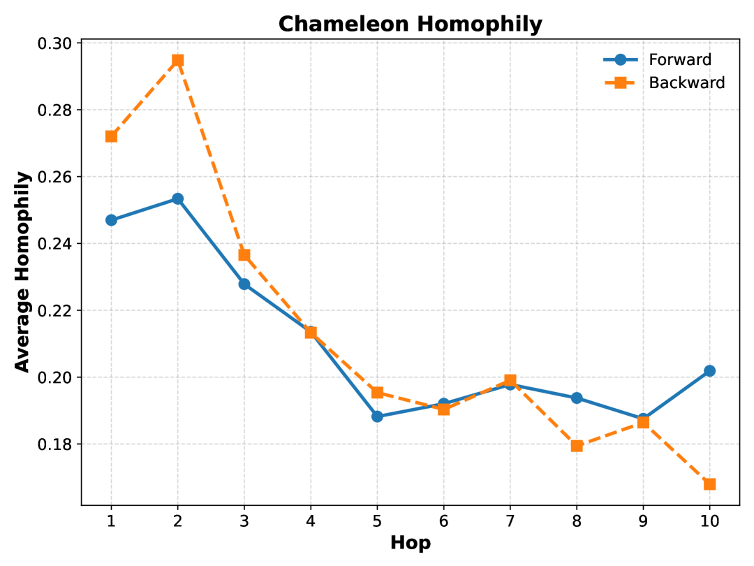
((a)) The homophily fluctuation in Chameleon.

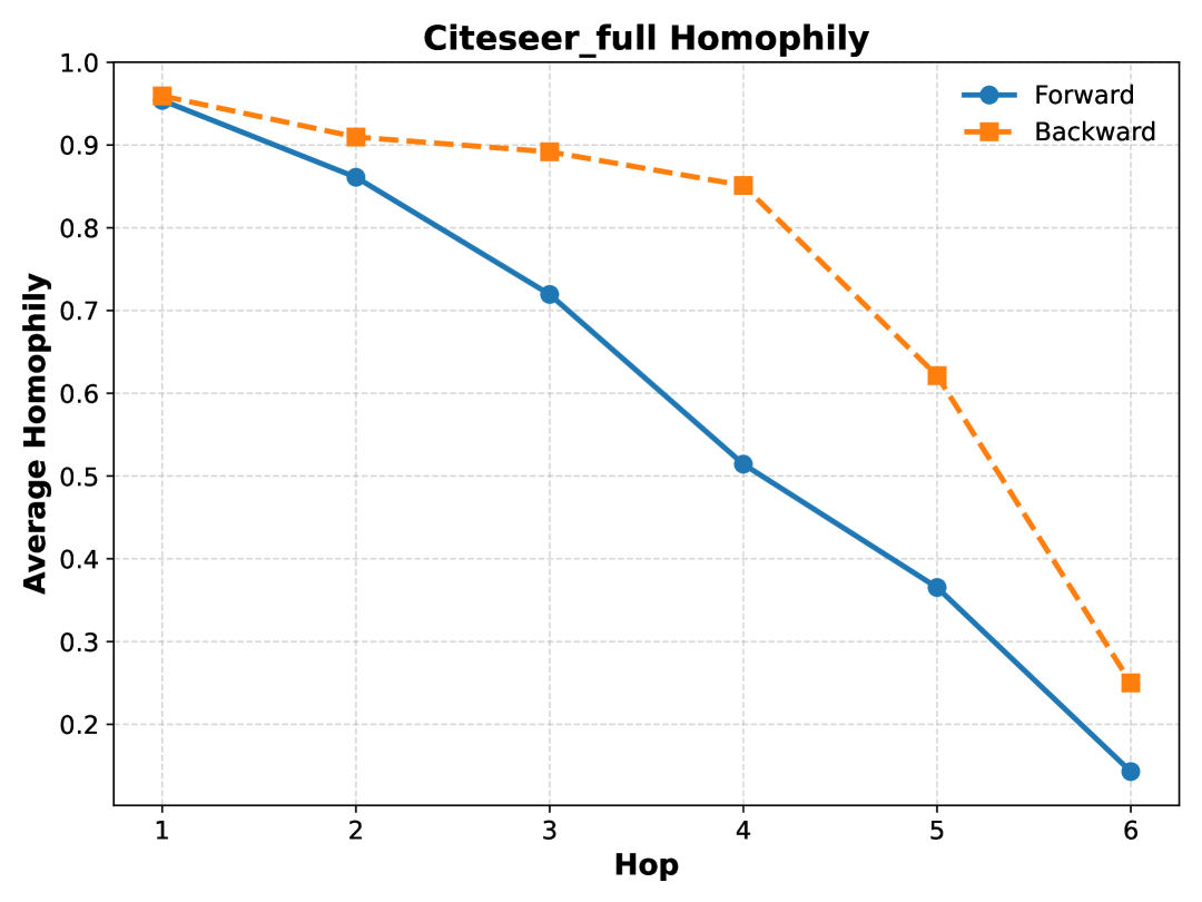
((b)) The directional homophily difference in Citeseer-Full.

Figure 1: The average node-wise homophily ratio in different hops. Forward denotes the direction in which the graph is constructed while backward denotes the reverse direction. The line chart reveals (a) the homophily ratio does not consistently decrease with increasing distance, and (b) the homophily levels of forward and backward neighbors can be different.

In this paper, we propose Directed Homophily-aware Graph Neural Network (DHGNN), a novel framework designed to extract meaningful information from complex, noisy neighborhoods by explicitly modeling homophily fluctuations across hops, and structural as well as homophily gaps between opposite directions.

To address the challenges posed by heterophilic neighborhoods, we introduce a homophily-aware gating mechanism that dynamically adjusts gating values for message-passing based on the embedding similarity and informativeness of neighboring nodes across different hops. This design enables the model to handle fluctuating homophily patterns and selectively incorporate relevant signals, even from distant neighbors.

To capture the structural and homophily differences between opposite directions, we design a dual-encoder architecture that separately processes the forward and backward directions of directed graphs. A structure-aware, noise-tolerant fusion mechanism then adaptively integrates the directional embeddings, guided by both node-level features and structural context, to form a unified and expressive node representation. By employing independent encoders along with branch-specific auxiliary losses, the model effectively captures distinct and meaningful information from each direction.

To validate the effectiveness of DHGNN, we conduct comprehensive experiments on five benchmark datasets with varying levels of homophily and directionality. DHGNN is able to outperform state-of-the-art baselines in node classification and link prediction tasks. Further analysis demonstrates its ability to adaptively respond to both the homophily fluctuations across hops and the directional homophily gaps. An analysis of DHGNN’s behavior at deeper layers suggests that the model effectively alleviates the over-smoothing issue.

Our key contributions can be summarized as follows:

• We propose a homophily-aware gating mechanism that adaptively regulates message-passing weights across layers and directions.

• We develop a structure-aware, noise-tolerant fusion strategy that integrates directional embeddings into a unified representation.

• We validate the proposed DHGNN on five heterophilic and homophilic datasets. The results demonstrate improved classification and link prediction performance by up to 15.07%, along with interpretable gate behavior.

2 Related Work

Graph Neural Networks for heterophilic graphs. Various methods have been developed to handle heterophily in graphs. LINKX (Lim et al., 2021) avoids aggregating over heterophilic neighborhoods by separately processing node features and adjacency information. Other approaches decompose ego and neighbor representations or utilize signal separation techniques (Zhu et al., 2020a; Suresh et al., 2021; He et al., 2022; Li et al., 2022a; Luan et al., 2022). For example, H2GCN (Zhu et al., 2020a) concatenates information from different neighborhood ranges while excluding self-loops. WRGNN (Suresh et al., 2021) and BM-GCN (He et al., 2022) apply different transformation matrices to ego and neighbor messages. GloGNN (Li et al., 2022a) uses both low- and high-pass filters, while ACM-GCN (Luan et al., 2022) distinguishes ego embeddings using identity filters at the channel level.

Several methods employ adaptive weighting strategies. GPR-GNN (Chien et al., 2020) learns Generalized PageRank weights across layers. GGCN (Yan et al., 2022) uses learnable scalars for self and signed neighbor edges. Gradient Gating ($G^{2}$)(Rusch et al., 2022) introduces multi-rate gradient flow, and Ordered GNN(Song et al., 2023) applies soft gating to gradually freeze node embeddings and mitigate over-smoothing. However, most gating-based approaches assume a monotonically decreasing homophily with distance, overlooking potential fluctuations, which may limit the ability to extract informative signals from distant nodes.

Directed Graph Neural Networks. Traditional GNNs often convert directed graphs into undirected ones, potentially disrupting important inter-class links (see Appendix A for an example). To address this limitation, various methods have been developed from both spectral and spatial perspectives to explicitly model directionality in graph learning. Spectral approaches include DiGCN (Tong et al., 2020a), which approximates the Laplacian using personalized PageRank transition probabilities, and MagNet (Zhang et al., 2021), which introduces a Magnetic Laplacian with complex-valued phase matrices to encode directionality. Building on this, Geisler et al. (2023) use both the Magnetic Laplacian and directional random walk encodings as positional encodings for Transformers, while Huang et al. (2024b) further enhance the Magnetic Laplacian-based encoding with additional structural factors. However, these methods often apply the same transformation to both edge directions, overlooking directional differences in neighborhood homophily.

Spatial approaches explicitly separate directional representations. DGCN (Tong et al., 2020b) uses distinct functions for first- and second-order proximity. Dir-GNN (Rossi et al., 2024) independently encodes each direction and combines them with manually set fusion weights, while NDDGNN (Huang et al., 2024a) adaptively learns fusion weights based on structural and feature similarities. Although effective for local interactions, such layer-wise fusion may struggle to capture long-range dependencies along extended paths.

3 Preliminaries

Directed graphs. In this paper, we address the tasks of semi-supervised node classification and link prediction on attributed directed graphs. Given a directed graph $\mathcal{G}=(\mathcal{V},\mathbf{X},\mathbf{A})$ with $n$ nodes and $m$ edges, each node $i\in\mathcal{V}$ is associated with a feature vector, forming a feature matrix $\mathbf{X}\in\mathbb{R}^{n\times d}$, where $d$ is the feature dimension. The graph also includes a label $y_{i}\in\{1,\dots,C\}$ for each node corresponding to $C$ classes. The directed structure is represented by an adjacency matrix $\mathbf{A}\in\{0,1\}^{n\times n}$, where $\mathbf{a}_{ij}=1$ if there is a directed edge from node $i$ to node $j$, and zero otherwise.

Message-passing neural networks. Most GNNs follow a message passing mechanism (Xu et al., 2018) iteratively updating node representations of node $v$, namely $\mathbf{{h}}^{(l)}_{v}\in\mathbb{R}^{p}$, where $l$ denotes the layer number and $p$ is the hidden dimension at current layer. Each layer of a message passing GNN comprises two fundamental steps, i.e., aggregation and combination, which can be formulated as:

$$\mathbf{m}^{(l)}_{v} =\text{AGGREGATE}^{(l)}(\{\mathbf{h}^{(l-1)}_{u}|u\in\mathcal{N}(v)\}),$$ (1)

$$\mathbf{h}^{(l)}_{v} =\text{COMBINE}^{(l)}(\mathbf{h}^{(l-1)}_{v},\mathbf{m}^{(l)}_{v}),$$

where the $\text{AGGREGATE}(\cdot)$ takes the embeddings of nodes in the neighborhood $\mathcal{N}(v)$ of a node $v$ and generates a message $\mathbf{m}^{(l)}_{v}$, and $\text{COMBINE}(\cdot)$ incorporates the message with the previous node embedding $\mathbf{h}^{(l-1)}_{v}$ to produce the updated embedding $\mathbf{h}^{(l)}_{v}$. The initial embedding $\mathbf{h}^{(0)}_{v}$ is set to be the original node feature $\mathbf{x}_{v}$ of node $v$.

4 Methodology

4.1 Model architecture

To enable the model to effectively handle varying levels of homophily in the forward and backward directions, we propose a novel and effective framework specifically designed to disentangle and adaptively integrate directional information, namely DHGNN as shown in Figure 2a.

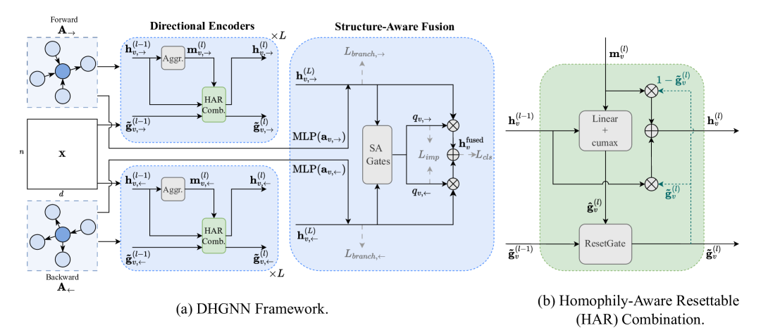
Figure 2: The framework of DHGNN. “SA Gates” is short for the structure-aware noise-tolerant gates. The model consists of two message-passing modules (one for each edge direction) and a fusion module. Node representations are learned independently for the forward and backward directions, and subsequently fused into a unified representation.

The model employs two parallel encoders based on a resettable gated message-passing scheme. The two encoders share the same architecture but with independent parameters, which are responsible for processing forward and backward edges, respectively. Within each encoder, a gating vector dynamically regulates the contribution of incoming messages. The resettable gating mechanism is designed to attenuate or amplify messages based on their informativeness, particularly preserving informative long-range dependencies. This enables the model to propagate relevant information more effectively across multiple hops.

The directional embeddings are then combined using a structure-aware fusion mechanism. Fusion gating values are derived from both directional embeddings and structural cues from the directed adjacency matrices, allowing the model to integrate directional information based on graph topology.

To avoid the collapse of the two directional encoders into a single dominant pathway, DHGNN introduces an auxiliary importance loss that discourages extreme imbalance in the fusion decision scores. Furthermore, to encourage disentanglement and minimize redundancy between the forward and backward encoders, a branch classification loss is incorporated during training.

4.2 Homophily-aware gated message passing

As presented in the previous sections, the homophily ratio could vary in the backward and forward directions, and the homophily ratio is not strictly decreasing in all datasets.

Therefore, to capture fluctuations in local homophily and gaps between forward and backward directions simultaneously, we introduce a homophily-aware gated message-passing mechanism, as defined in Eq. (2), while the gating strategy at the combination step is inspired by Ordered GNN (Song et al., 2023). In each aggregation layer, a separate gating vector is updated with a homophily-aware resettable (HAR) combination module alongside the node embeddings (shown in Figure 2b), modulating the influence of forward messages from the neighborhood in a node-specific manner.

$$\small\begin{split}\mathbf{m}_{v}^{(l)}&=\text{mean}\left(\left\{\mathbf{h}_{u}^{(l-1)}|u\in\mathcal{N}(v)\right\}\right),\\ \mathbf{\hat{g}}_{v}^{(l)}&=\text{cumax}_{\leftarrow}\left(\mathbf{W}^{(l)}\left[\mathbf{h}_{v}^{(l-1)}||\mathbf{m}_{v}^{(l)}\right]+\mathbf{b}^{(l)}\right),\\ \mathbf{\tilde{g}}_{v}^{(l)}&=\text{ResetGate}(\mathbf{\tilde{g}}_{v}^{(l-1)},\mathbf{\hat{g}}_{v}^{(l)}),\\ \mathbf{h}_{v}^{(l)}&=\mathbf{\tilde{g}}_{v}^{(l)}\circ\mathbf{h}_{v}^{(l-1)}+(1-\mathbf{\tilde{g}}_{v}^{(l)})\circ\mathbf{m}_{v}^{(l)},\end{split}$$ (2)

where $\text{cumax}_{\leftarrow}(\cdot)=\text{cumsum}_{\leftarrow}(\text{softmax}(\cdot))$ denotes a composite operation that applies the softmax function followed by a cumulative sum. The subscript $\leftarrow$ indicates that the accumulation proceeds in a reverse (right-to-left) direction. $\mathbf{W}^{(l)}$ and $\mathbf{b}^{(l)}$ are the learnable weight and bias term in the multilayer perceptron (MLP) layer, $||$ stands for concatenation, and $\circ$ denotes element-wise multiplication. The first equation represents the aggregation step in the message-passing layer, while the remaining three equations define the combination step.

The gating vector is updated using a Gated Recurrent Unit (GRU)-inspired resettable gating mechanism, which enables selective resetting of its values. The reset gate $\mathbf{r}_{v}^{(l)}$ is computed via an MLP conditioned on the current preliminary gating vector $\mathbf{\hat{g}}_{v}^{(l)}$ and the previous gating vector $\mathbf{\tilde{g}}_{v}^{(l-1)}$:

$$\small\begin{split}\mathbf{\tilde{g}}_{v}^{(l)}&=\text{ResetGate}(\mathbf{\tilde{g}}_{v}^{(l-1)},\mathbf{\hat{g}}_{v}^{(l)})=\left(1-\mathbf{r}_{v}^{(l)}\right)\circ\mathbf{\tilde{g}}_{v}^{(l-1)}+\mathbf{r}_{v}^{(l)}\circ\mathbf{\hat{g}}_{v}^{(l)},\\ \mathbf{r}_{v}^{(l)}&=\text{MLP}(\mathbf{W}_{r}\mathbf{\hat{g}}_{v}^{(l)}+\mathbf{U}_{r}\mathbf{\tilde{g}}_{v}^{(l-1)}+\mathbf{b}_{r}),\end{split}$$ (3)

where $\mathbf{W}_{r}$, $\mathbf{U}_{r}$ and $\mathbf{b}_{r}$ are the two learnable weights and bias term in the MLP, respectively. The values in the gating vector tend to increase when the forward neighborhood messages deviate from the current node embedding. These values are constrained within the range $[0,1]$, where higher values correspond to a reduced influence from neighborhood messages at the current layer. This selective suppression of information from heterophilic neighbors helps mitigate the over-smoothing issue commonly observed in heterophilic graphs.

To accommodate fluctuations in neighborhood homophily across different hop distances, the gating vector values are not constrained to follow a strictly increasing or decreasing trend across layers. This behavior is enabled by the resettable gating mechanism, which allows gating values to increase when the homophily ratio we infer from the embedding similarity decreases or when the incoming message is uninformative, and decrease otherwise. Such flexibility empowers the model to suppress information aggregation from all nodes in the hops with low homophily ratios, while still enabling the integration of informative signals from more distant nodes when necessary.

To prevent premature saturation of gating vectors during message passing and reduce the parameter count in the gating network, we employ a chunking strategy similar to the one in (Song et al., 2023).

4.3 Structure-aware noise-tolerant fusion

The representations learned from the forward and backward directions can differ significantly due to variations in neighborhood homophily and linking patterns. To fully exploit the information provided by each direction, we design a structure-aware noise-tolerant fusion mechanism. This mechanism integrates the directional node embeddings generated by two separate encoders, producing a unified representation before it is passed to downstream tasks. The fusion process is formulated as follows:

$$\small\begin{split}\mathbf{h}_{v}^{\text{fused}}=\sigma\left(q_{v,\leftarrow}\mathbf{h}^{(L)}_{v,\leftarrow}+q_{v,\rightarrow}\mathbf{h}^{(L)}_{v,\rightarrow}\right),\end{split}$$ (4)

where $\sigma(\cdot)$ is a linear layer, scalars $q_{v,\leftarrow}$ and $q_{v,\rightarrow}$ indicate the decision scores for each direction, and $L$ denotes the number of encoder layers. These scores are given by a noise-tolerant MLP-based gating mechanism (To simplify the notation, we omit the layer index $L$ and use only a single-direction subscript in the following equations, as the processing steps for the two directions are analogous.):

$$\small\begin{split}q_{v,\leftarrow},q_{v,\rightarrow}&=\text{Softmax}\left(\text{NTB}(\mathbf{\tilde{h}}_{v,\leftarrow}),\text{NTB}(\mathbf{\tilde{h}}_{v,\rightarrow})\right),\\ \mathbf{\tilde{h}}_{v,\leftarrow}&=\mathbf{h}_{v,\leftarrow}+\beta\text{MLP}(\mathbf{a}_{v,\leftarrow}),\\ \text{NTB}(\mathbf{\tilde{h}}_{v,\leftarrow})&=\mathbf{\tilde{h}}_{v,\leftarrow}\mathbf{W}_{1,\leftarrow}+\epsilon\cdot\text{Softplus}(\mathbf{\tilde{h}}_{v,\leftarrow}\mathbf{W}_{2,\leftarrow}),\end{split}$$ (5)

where $\text{NTB}(\cdot)$ stands for the noise-tolerant block, $\mathbf{a}_{v}$ is the corresponding vector in $\mathbf{A}$ containing all outgoing neighbors of $v$, and $\epsilon\sim N(0,1)$ denotes standard Gaussian noise. $\mathbf{W}_{1,\leftarrow},\mathbf{W}_{2,\leftarrow}\in\mathbb{R}^{p\times 1}$ are learnable weights that control clean and noisy scores, respectively. Since the adjacency matrix of a directed graph is asymmetric, it can provide richer structural information than its undirected counterpart. To fully leverage this asymmetric structure in guiding the fusion process, we incorporate an adjacency-based embedding, which has been proven effective as a structural embedding in LINKX (Lim et al., 2021), into the input of $\text{NTB}(\cdot)$. This integration is governed by the hyperparameter $\beta$.

To prevent two encoders from collapsing into one, we incorporate an importance loss following (Wang et al., 2023):

$$\small\begin{split}\text{Importance}(\mathbf{h}_{\leftarrow})&=\sum_{v\in\mathcal{V}}q_{v,\leftarrow},\\ \text{Importance}(\mathbf{h}_{\rightarrow})&=\sum_{v\in\mathcal{V}}q_{v,\rightarrow},\\ L_{imp}=\text{CV}(\text{Importance}(\mathbf{h}_{\leftarrow})&,\text{Importance}(\mathbf{h}_{\rightarrow}))^{2},\end{split}$$ (6)

where the importance score, $\text{Importance}(\cdot)$, is defined as the sum of decision scores $q_{v,\leftarrow}$ and $q_{v,\rightarrow}$ across all nodes in the same direction. Here, $\text{CV}(\cdot)$ denotes the coefficient of variation. Consequently, the importance loss $L_{imp}$ quantifies the variability of these importance scores, encouraging all encoders to maintain a comparable level of importance.

4.4 Objective function

The final objective function consists of three components. The primary component is the classification loss $L_{cls}$, computed using the fused node embedding $\mathbf{h}_{v}^{\text{fused}}$. We adopt focal loss for node classification and cross-entropy loss for link prediction.

The first auxiliary component is the importance loss $L_{imp}$, as described in the previous section. The second auxiliary component is the branch classification loss $L_{branch}$, which is calculated as the average of classification losses from each directional branch. Formally, $L_{branch}=(L_{branch,\leftarrow}+L_{branch,\rightarrow})/2$. We adopt cross-entropy loss for both directions.

To prevent the fusion mechanism from interfering with the individual optimization of each directional encoder, we apply stop-gradient operations to the directional embeddings after computing their respective losses and before they are fused into the final output. The two auxiliary losses are weighted by hyperparameters $\lambda_{1}$ and $\lambda_{2}$, respectively. Thus, the overall objective function is formulated as:

$$\small\begin{split}L_{total}=(1-\lambda_{2})(L_{cls}+\lambda_{1}L_{imp})+\lambda_{2}L_{branch}.\end{split}$$ (7)

5 Experimental Results

5.1 Datasets

We evaluate the performance of our model on two homophilic datasets and three heterophilic datasets, with varying graph densities. The homophilic datasets include Cora-ML and Citeseer-Full (Bojchevski and Günnemann, 2017), while the heterophilic datasets comprise Chameleon, Squirrel (Pei et al., 2020), and Roman-Empire (Platonov et al., 2023). Additional dataset details are provided in the Appendix B.

5.2 Experimental setup

The baseline models used for comparison fall into three categories: (1) Traditional undirected graph methods, such as GCN (Kipf and Welling, 2016), and GAT (Veličković et al., 2017); (2) State-of-the-art undirected graph methods for heterophilic graphs, including H2GCN (Zhu et al., 2020a), GPRGNN (Chien et al., 2020), LINKX (Lim et al., 2021), FSGNN (Maurya et al., 2021), ACM-GCN (Luan et al., 2022), GloGNN (Li et al., 2022a), and $G^{2}$ (Gradient Gating) (Rusch et al., 2022); and (3) State-of-the-art directed graph methods, comprising DiGCN (Tong et al., 2020a), MagNet (Zhang et al., 2021), Dir-GNN (Rossi et al., 2024), and NDDGNN (Huang et al., 2024a).

For those baselines with results reported in (Huang et al., 2024a), we adopt the results in the paper. For DHGNN, we select the best hyperparameters from 100 runs using the Optuna hyperparameter optimization framework (Akiba et al., 2019). The selected hyperparameters are detailed in Appendix C.

5.3 Node classification

Table 1: Node classification accuracy (%) across homophilic and heterophilic datasets. The best results are highlighted in bold, while the second-best results are marked with underline.

Datasets	Cora-ML	Citeseer-Full	Chameleon	Squirrel	Roman-Empire
MLP	77.48$\pm$1.23	80.01$\pm$1.23	46.36$\pm$2.57	34.14$\pm$1.94	65.76$\pm$0.42
GCN	52.37$\pm$1.77	54.65$\pm$1.22	64.82$\pm$2.24	53.43$\pm$2.01	73.69$\pm$0.74
GAT	54.12$\pm$1.56	55.15$\pm$1.31	45.56$\pm$3.16	39.14$\pm$2.88	71.16$\pm$0.63
GraphSAGE	54.12$\pm$1.56	55.15$\pm$1.31	45.56$\pm$3.16	39.14$\pm$2.88	71.16$\pm$0.63
H2GCN	62.86$\pm$1.45	68.34$\pm$1.36	59.39$\pm$0.98	37.90$\pm$0.02	60.11$\pm$0.52
GPRGNN	68.88$\pm$1.66	70.12$\pm$1.24	62.85$\pm$2.90	54.35$\pm$0.87	64.85$\pm$0.27
ACM-GCN	69.96$\pm$1.53	73.61$\pm$1.32	74.76$\pm$2.20	67.40$\pm$2.21	69.66$\pm$0.62
GloGNN	73.78$\pm$1.69	76.13$\pm$1.14	57.88$\pm$1.76	71.21$\pm$1.84	59.63$\pm$0.69
LINKX	72.32$\pm$1.41	78.75$\pm$1.34	68.42$\pm$1.32	61.81$\pm$1.80	37.55$\pm$0.36
FSGNN	67.51$\pm$1.65	66.35$\pm$1.16	78.27$\pm$1.28	74.10$\pm$1.89	79.92$\pm$0.56
$G^{2}$	76.63$\pm$1.63	80.36$\pm$1.18	71.40$\pm$2.38	64.26$\pm$2.38	82.16$\pm$0.78
Di-GCN	87.36$\pm$1.06	92.75$\pm$0.75	52.24$\pm$3.65	37.74$\pm$1.54	52.71$\pm$0.32
MagNet	85.26$\pm$1.05	93.38$\pm$0.89	58.32$\pm$2.87	39.01$\pm$1.93	88.07$\pm$0.27
Dir-GNN	84.45$\pm$1.69	92.79$\pm$0.59	79.71$\pm$1.26	75.31$\pm$1.92	91.23$\pm$0.32
NDDGNN	88.14$\pm$1.28	94.17$\pm$0.58	79.79$\pm$1.04	75.38$\pm$1.95	91.76$\pm$0.27
DHGNN (ours)	88.39$\pm$0.98	94.60$\pm$0.52	80.11$\pm$1.73	76.84$\pm$1.61	89.05$\pm$0.53

Table 2: Link prediction accuracy (%) on homophilic and heterophilic graphs. The best results are highlighted in bold, while the second-best results are marked with underline.

Datasets	Cora-ML	Citeseer-Full	Chameleon	Squirrel
GCN	76.24$\pm$4.25	71.16$\pm$4.41	86.03$\pm$1.53	90.64$\pm$0.49
GAT	64.58$\pm$12.28	67.28$\pm$2.90	85.12$\pm$1.57	90.37$\pm$0.45
MagNet	82.20$\pm$3.36	85.89$\pm$4.61	86.28$\pm$1.23	90.13$\pm$0.53
Dir-GNN	82.23$\pm$4.01	70.62$\pm$6.56	82.76$\pm$2.72	89.17$\pm$0.52
NDDGNN	83.04$\pm$9.56	87.93$\pm$3.92	90.30$\pm$1.82	92.40$\pm$1.01
DHGNN (ours)	98.11$\pm$1.84	89.70$\pm$6.76	99.09$\pm$2.02	96.21$\pm$3.42

We evaluate our model on five datasets using the same data splits as in (Huang et al., 2024a). The results, presented in Table 1, report the mean classification accuracy on the test nodes over 10 random splits.

Compared to methods designed for undirected heterophilic graphs, our proposed model consistently outperforms all undirected baselines. Specifically, it achieves average absolute improvements of 11.76%, 14.24%, 1.84%, 2.74% and 6.89% across the five datasets when compared to the strongest undirected method on each. It can be observed that MLP outperforms some of the GNN-based methods on directed datasets such as Cora-ML and Citeseer-Full. This suggests that these methods may struggle to effectively leverage structural information for node classification on directed graphs.

In addition, our model surpasses existing state-of-the-art methods tailored for directed graphs on four out of the five datasets. Take the heterophilic Squirrel dataset as an example. It exhibits the highest graph density and the lowest homophily ratio among the five datasets, indicating more complex inter-class linking patterns. The improvements on this dataset highlight our model’s strong ability to leverage inter-class connections effectively. The performance variation on Roman-Empire may be attributed to the distinct nature of this graph, which is based on semantic relationships between words rather than hyperlinks or citations. In the Roman-Empire dataset, two words are connected if they appear consecutively or are linked via the dependency tree of a sentence. This construction may reduce both the directional asymmetry and the long-range dependencies between words, thereby limiting DHGNN’s ability to extract useful information for node classification.

5.4 Link prediction

In addition to node classification, we assess the performance of the proposed DHGNN on link prediction tasks. Results are reported in Table 2. Our model achieves the highest prediction accuracy across all datasets, with absolute improvements of 15.07%, 1.77%, 8.79%, and 3.81% over the best-performing baseline on each dataset, respectively. These results indicate that the proposed method effectively captures structural information from directed neighborhoods. This may be attributed to the fact that DHGNN maintains independent encoders for each direction, rather than performing fusion after every message passing layer in NDDGNN. This design enables each encoder to capture long-range dependencies along extended paths more effectively, thereby providing richer structural information for link prediction.

5.5 Ablation study

Table 3: Ablation study for node classification. The best result (accuracy) is highlighted in bold. +ResGate denotes the resettable homophily-aware gating mechanism for message passing, and +Fusion denotes the structure-aware fusion module.

+ResGate	+Fusion	+$L_{branch}$	+$L_{imp}$	Chameleon	Squirrel	Roman-Empire
-	-	-	-	79.21$\pm$1.03	74.96$\pm$1.95	43.35$\pm$0.63
✓	-	-	-	79.52$\pm$1.38	75.22$\pm$2.13	85.55$\pm$0.46
✓	✓	-	-	79.98$\pm$1.68	76.38$\pm$1.57	86.50$\pm$0.36
✓	✓	✓	-	79.54$\pm$1.17	76.25$\pm$1.84	88.06$\pm$0.44
✓	✓	✓	✓	80.11$\pm$1.73	76.84$\pm$1.61	89.05$\pm$0.53

To evaluate the effectiveness of different components in our proposed framework, we conduct an ablation study focusing on four key elements: the resettable homophily-aware gating mechanism (ResGate), the structure-aware noise-tolerant fusion module (Fusion), and the two auxiliary losses, i.e., $L_{branch}$ and $L_{imp}$. When all components are disabled (the first row in Table 3), the model degenerates to a two-branch vanilla GCN that encodes each direction individually, and a linear layer followed by summation as the alternative fusion module. The results in Table 3 demonstrate that the homophily-aware gating mechanism significantly improves performance on heterophilic datasets. Additionally, the structure-aware fusion module enhances the extraction of valuable information from the directional encoders. The results also suggest that the combined use of the two auxiliary losses can lead to synergistic effects, further boosting classification accuracy.

5.6 Visualization of gating vectors

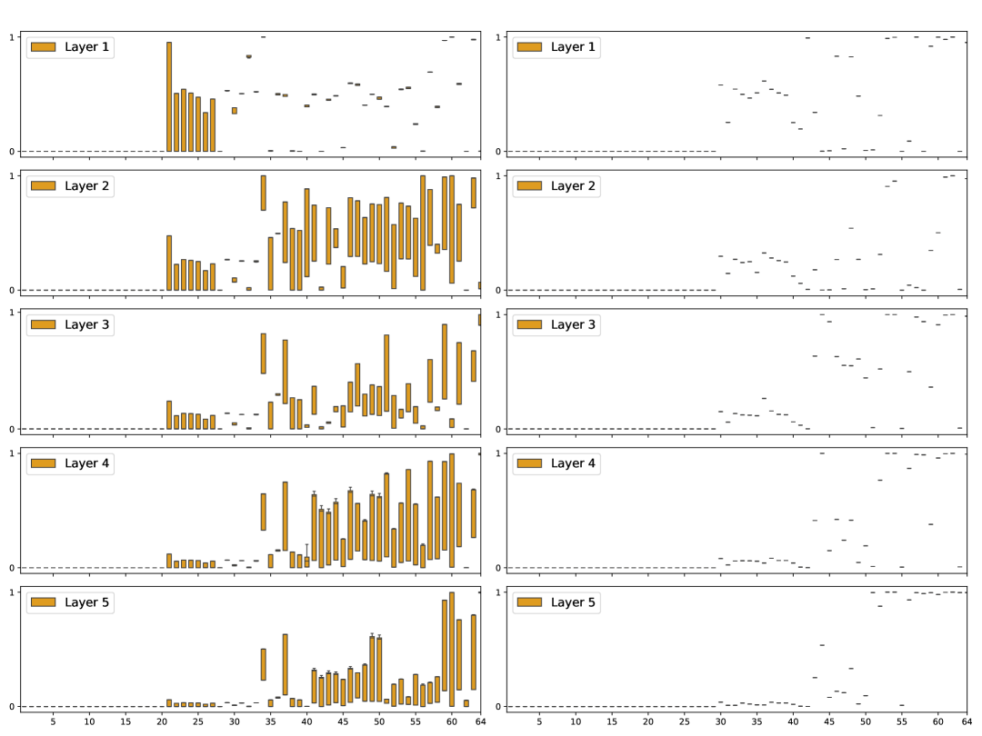
((a)) Forward/backward gating values on Chameleon.

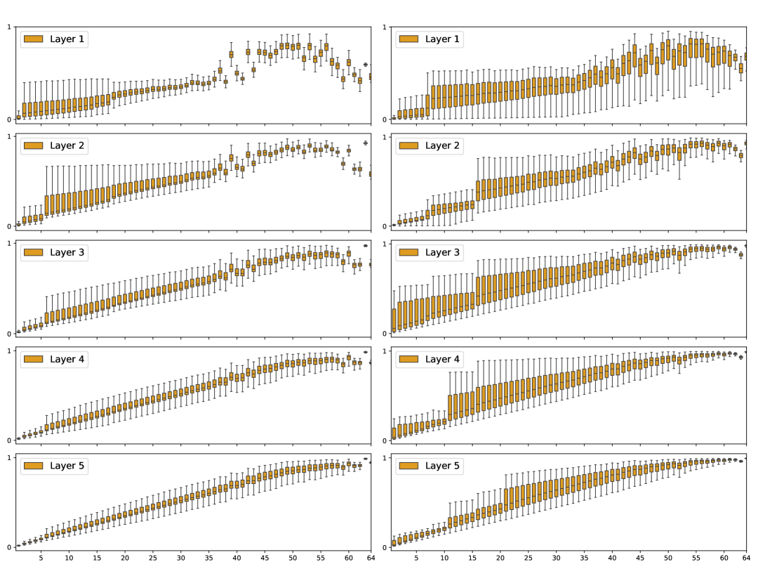
((b)) Forward/backward gating values on Citeseer-Full.

Figure 3: The gating values of the first five layers on heterophilic and homophilic datasets.

To better understand the behavior of our homophily-aware gated message passing mechanism, we visualize the gating values on two representative datasets: the heterophilic Chameleon and the homophilic Citeseer-Full, as shown in Figure 3. A clear gap in gating values between the two directions is observed on Chameleon, highlighting a strong directional asymmetry. While a similar trend is present on Citeseer-Full, the gap is notably smaller, suggesting that the gating mechanism adaptively responds to the directional differences in homophily on different types of graphs.

Additionally, we observe a consistent decrease in most gating values from layer 1 to layer 2 on the Chameleon dataset. This aligns with the higher homophily ratio at the second hop, as illustrated in Figure 1(a). The larger variance in gating values, as indicated by the taller boxplots, may be attributed to the increased variability in neighborhood homophily at greater hop distances. These findings indicate that the proposed gating mechanism not only distinguishes between directional neighborhoods but also dynamically adapts to the non-monotonic variations in homophily across layers. Similar gating behavior is observed on other datasets, as visualized in Appendix D.

5.7 Alleviating Over-smoothing in DHGNN

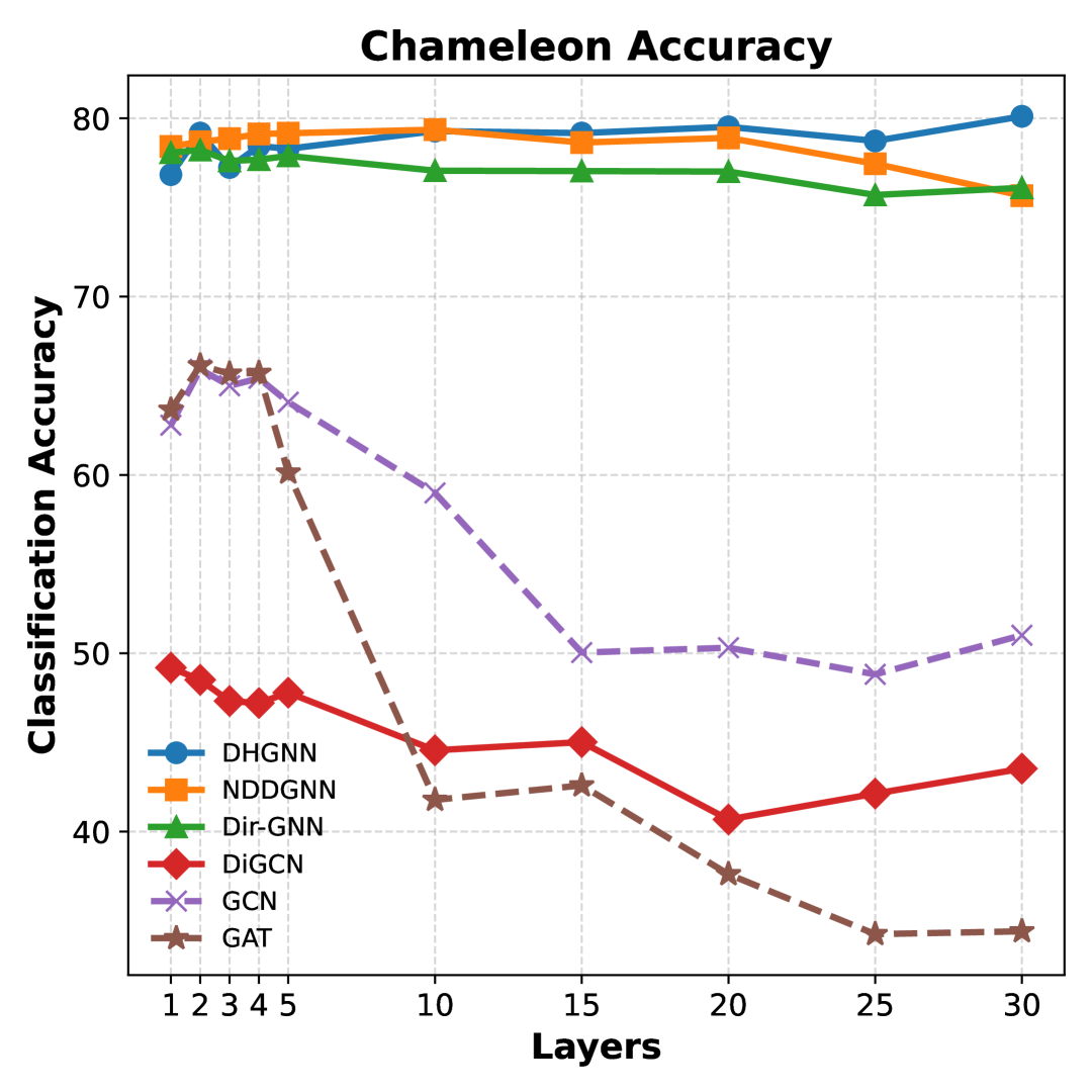
((a)) Node classification accuracy on Chameleon at deeper layers, better visualised in color.

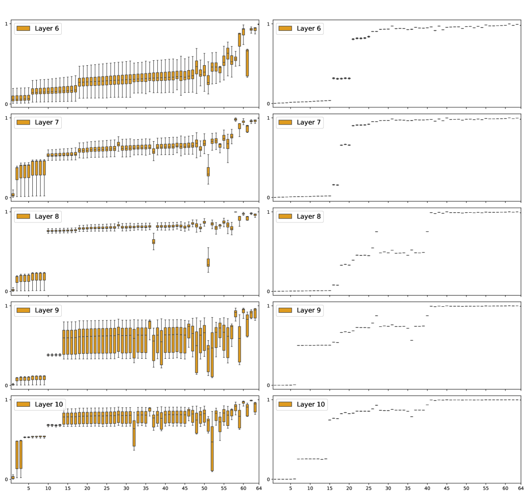
((b)) Gating values on Chameleon at deeper layers.

Figure 4: The node classification accuracy and behavior of gating values at deeper layers.

As shown in Figure 4(a), DHGNN effectively mitigates the over-smoothing problem. Node classification accuracy does not decrease, and even slightly improves, as the model goes deeper. The change in accuracy is obviously smaller than that observed in traditional GNNs, and remains lower than other baselines. Analysis of the gating vectors at deeper layers (Figure 4(b)) shows that while some gates saturate and refuse neighborhood messages, others remain open with lower values. This suggests that the model continues to capture informative signals from distant nodes, even at greater depths.

6 Conclusion

We introduced Directed Homophily-aware Graph Neural Network (DHGNN), a novel framework that adaptively integrates neighborhood information by accounting for both homophily gaps between opposite directions and homophily fluctuations across layers. DHGNN features a homophily-aware gating mechanism with a resettable update strategy and a structure-aware, noise-tolerant fusion module that selectively emphasizes informative directional representations. Comprehensive experiments on both homophilic and heterophilic datasets show that DHGNN can outperform state-of-the-art methods on node classification and link prediction tasks. Gating analyses further confirm its ability to adaptively respond to complex homophily patterns. Our method not only advances effective learning on directed graphs but also introduces a robust mechanism for extracting informative signals from obscure or noisy neighborhoods.

While DHGNN demonstrates to be effective, its scalability on extremely large graphs and generalization to broader domains beyond citation and web graphs remain promising directions for future exploration. We aim to further enhance the model’s efficiency and extend its applicability across diverse graph domains, paving the way for broader adoption in real-world scenarios.

Appendix A Differences Between Directed and Undirected Graphs

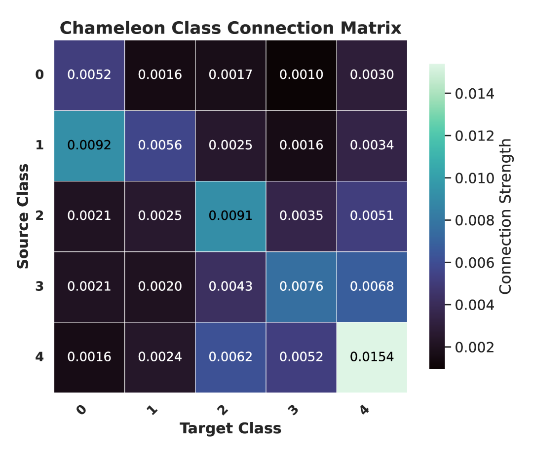
((a)) Directed Chameleon dataset.

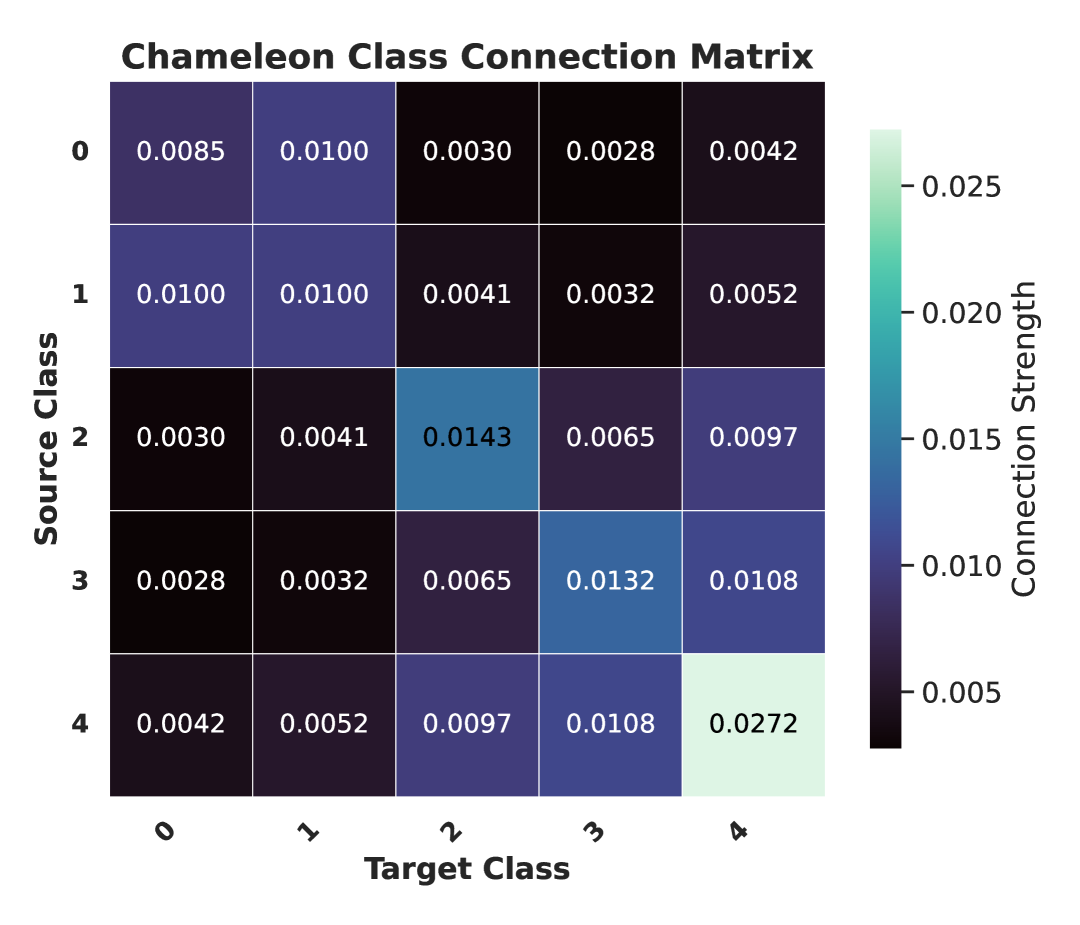
((b)) Undirected Chameleon dataset.

Figure A1: Class connection matrices of the directed and undirected versions of the same graph. The matrices tend to be asymmetric for heterophilic graphs, such as Chameleon.

Figure A1 illustrates how converting a directed graph to an undirected one can disrupt original inter-class connectivity patterns. In the heterophilic Chameleon dataset, this conversion removes the asymmetry between the edge ratios from class 1 to class 0 and vice versa, despite these ratios differing significantly in the original directed graph.

Appendix B Dataset Description

We provide detailed information on how each graph is constructed, along with their respective properties and statistics below:

Chameleon [Pei et al., 2020]: This dataset represents a Wikipedia page-page network on the topic of chameleons. Nodes correspond to Wikipedia articles, and edges denote mutual links between these articles. Node features indicate the presence of particular nouns in the articles. The nodes are classified into five categories based on their average monthly traffic. This dataset contains 2,277 nodes and 36,101 edges.

Squirrel [Pei et al., 2020]: Similar to the Chameleon dataset, the Squirrel dataset represents a Wikipedia page-page network, but on the topic of squirrels. It also consists of nodes representing Wikipedia articles and edges representing mutual links. Node features are based on the presence of informative nouns in the text of the articles. The Squirrel dataset has 5,201 nodes and 217,073 edges.

Cora-ML [Bojchevski and Günnemann, 2017]: This dataset is a citation network where nodes represent scientific publications, and edges represent citations between them. The dataset is derived from the Cora dataset, but with multi-label classification. It contains 2,995 nodes and 8,416 edges. Each node is assigned multiple labels that represent the categories of the papers.

Citeseer-Full [Bojchevski and Günnemann, 2017]: The Citeseer-Full dataset is another citation network where nodes represent scientific publications and edges represent citations between them. This dataset includes the entire Citeseer dataset without filtering. It contains 3,312 nodes and 4,732 edges, with each node labeled according to its category.

Roman-Empire [Platonov et al., 2023]: The dataset is based on the Roman Empire article from English Wikipedia, which was selected since it is one of the longest articles on Wikipedia. Each node in the graph corresponds to one (non-unique) word in the text. Thus, the number of nodes in the graph is equal to the article’s length. Two words are connected with an edge if at least one of the following two conditions holds: either these words follow each other in the text, or these words are connected in the dependency tree of the sentence (one word depends on the other). It contains 22662 nodes and 32927 edges. The class of a node is its syntactic role (The 17 most frequent roles were selected as unique classes and group all the other roles into the 18th class). For node features, the dataset uses FastText word embeddings [Grave et al., 2018].

Table A1: Dataset properties and statistics.

	Cora-ML	Citeseer-Full	Chameleon	Squirrel	Roman-Empire
#Nodes	2,995	4,230	2,277	5,201	22,662
#Edges	8,416	5,358	36,101	217,073	44,363
#Features	2,879	602	2,325	2,089	300
#Classes	7	6	5	5	18
Edge Hom.	0.792	0.949	0.235	0.223	0.500

Appendix C Experiment Settings

Data splits. We evaluate the performance by node classification accuracy with standard deviation in the semi-supervised setting. For Squirrel and Chameleon, we use 10 public splits (48%/32%/20% for training/validation/testing) provided by [Pei et al., 2020]. For the remaining datasets, we adopt the same splits as [Rossi et al., 2024]. For link prediction, the data splits are the same as in [Huang et al., 2024a].

Hardware information. We conduct our experiments on an Intel Core i9-10940X CPU and 2 NVIDIA RTX A5000 GPUs.

Hyperparameter settings. The hyperparameter settings of the proposed DHGNN are presented in Table A2.

Table A2: Hyperparameter settings for different datasets.

Hyperparameter	Chameleon	Squirrel	Cora-ML	Citeseer-Full	Roman-Empire
lr	0.05	0.01	0.001	0.005	0.005
wd	0.0001	0.0001	1e-6	0.0005	5e-6
GNN layers	12	5	4	14	6
gate_mlp layers	3	2	2	2	2
adj_mlp layers	4	2	2	2	4
input_fc dropout	0.5	0.5	0.5	0.5	0.3
dropout rate	0.3	0.3	0.2	0.0	0.1
adj_coef $\beta$	0.5	0.5	0	0.4	0
imp_coef $\lambda_{1}$	1e-5	1e-7	1e-3	1e-7	1e-3
branch_coef $\lambda_{2}$	0.95	0.8	0.9	0.95	0.05

Appendix D Visualization of the Gating Vectors on the Other Datasets

In addition to the visualization in Figure 3, Figure A2 presents gating values from other datasets, further illustrating the directional variance and the changes across different layers.

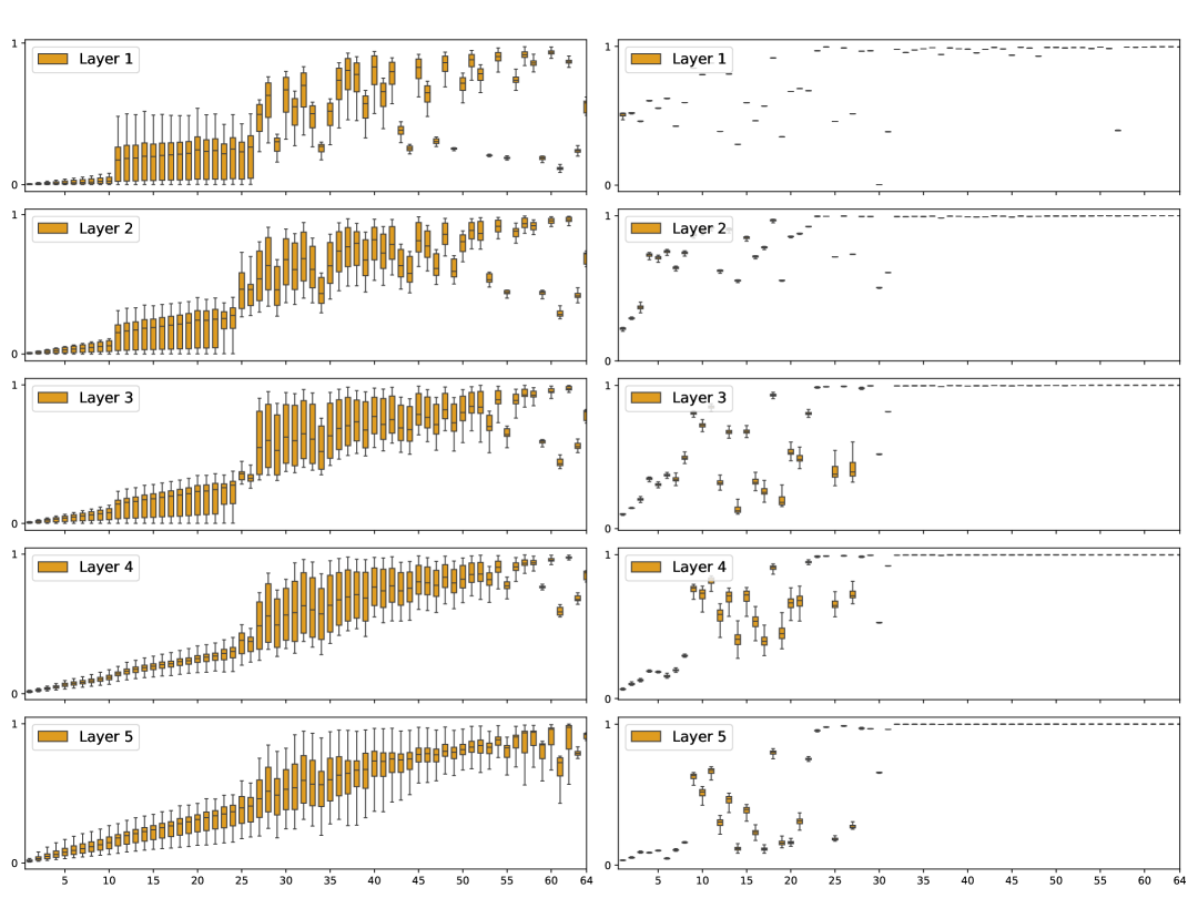
((a)) Forward/backward gating values on Squirrel.

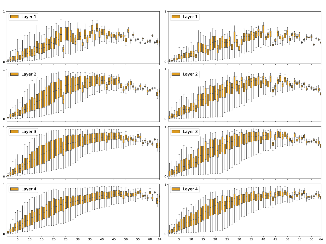
((b)) Forward/backward gating values on Cora-ML.

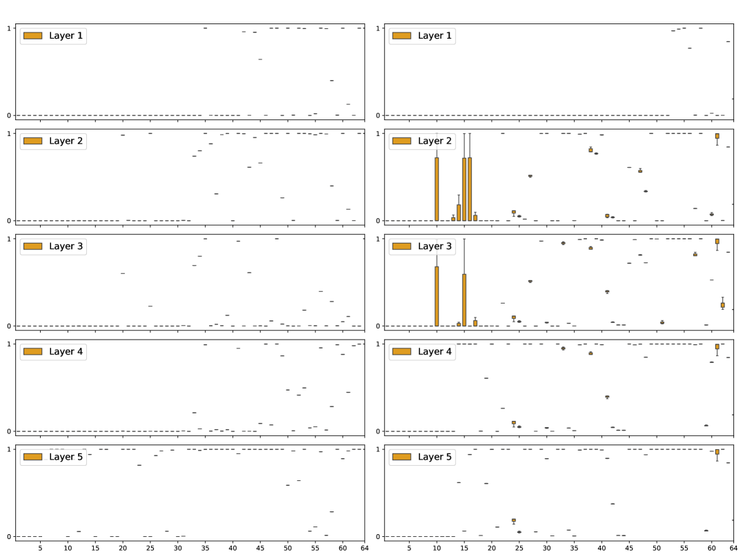
((c)) Forward/backward gating values on Roman-Empire.

Figure A2: The gating values of the first five layers on the other datasets.

References

- Akiba et al. [2019] T. Akiba, S. Sano, T. Yanase, T. Ohta, and M. Koyama. Optuna: A next-generation hyperparameter optimization framework. In The 25th ACM SIGKDD International Conference on Knowledge Discovery & Data Mining, pages 2623–2631, 2019.
- Bojchevski and Günnemann [2017] A. Bojchevski and S. Günnemann. Deep gaussian embedding of graphs: Unsupervised inductive learning via ranking. arXiv preprint arXiv:1707.03815, 2017.
- Chien et al. [2020] E. Chien, J. Peng, P. Li, and O. Milenkovic. Adaptive universal generalized pagerank graph neural network. arXiv preprint arXiv:2006.07988, 2020.
- Geisler et al. [2023] S. Geisler, Y. Li, D. J. Mankowitz, A. T. Cemgil, S. Günnemann, and C. Paduraru. Transformers meet directed graphs. In International conference on machine learning, pages 11144–11172. PMLR, 2023.
- Gilmer et al. [2017] J. Gilmer, S. S. Schoenholz, P. F. Riley, O. Vinyals, and G. E. Dahl. Neural message passing for quantum chemistry. In International conference on machine learning, pages 1263–1272. PMLR, 2017.
- Grave et al. [2018] E. Grave, P. Bojanowski, P. Gupta, A. Joulin, and T. Mikolov. Learning word vectors for 157 languages. Language Resources and Evaluation,Language Resources and Evaluation, Feb 2018.
- Hamilton et al. [2017] W. Hamilton, Z. Ying, and J. Leskovec. Inductive representation learning on large graphs. Advances in neural information processing systems, 30, 2017.
- He et al. [2022] D. He, C. Liang, H. Liu, M. Wen, P. Jiao, and Z. Feng. Block modeling-guided graph convolutional neural networks. In Proceedings of the AAAI conference on artificial intelligence, volume 36, pages 4022–4029, 2022.
- Huang et al. [2024a] J. Huang, Y. Mo, P. Hu, X. Shi, S. Yuan, Z. Zhang, and X. Zhu. Exploring the role of node diversity in directed graph representation learning. In Proceedings of the Thirty-Third International Joint Conference on Artificial Intelligence, pages 2072–2080, 2024a.
- Huang et al. [2024b] Y. Huang, H. Wang, and P. Li. What are good positional encodings for directed graphs? arXiv preprint arXiv:2407.20912, 2024b.
- Khemani et al. [2024] B. Khemani, S. Patil, K. Kotecha, and S. Tanwar. A review of graph neural networks: concepts, architectures, techniques, challenges, datasets, applications, and future directions. Journal of Big Data, 11(1):18, 2024.
- Kipf and Welling [2016] T. N. Kipf and M. Welling. Semi-supervised classification with graph convolutional networks. arXiv preprint arXiv:1609.02907, 2016.
- Li et al. [2018] Q. Li, Z. Han, and X.-M. Wu. Deeper insights into graph convolutional networks for semi-supervised learning. In Proceedings of the AAAI conference on artificial intelligence, volume 32, 2018.
- Li et al. [2022a] X. Li, R. Zhu, Y. Cheng, C. Shan, S. Luo, D. Li, and W. Qian. Finding global homophily in graph neural networks when meeting heterophily. In International Conference on Machine Learning, pages 13242–13256. PMLR, 2022a.
- Li et al. [2022b] X. Li, R. Zhu, Y. Cheng, C. Shan, S. Luo, D. Li, and W. Qian. Finding global homophily in graph neural networks when meeting heterophily. In International Conference on Machine Learning, pages 13242–13256. PMLR, 2022b.
- Lim et al. [2021] D. Lim, F. Hohne, X. Li, S. L. Huang, V. Gupta, O. Bhalerao, and S. N. Lim. Large scale learning on non-homophilous graphs: New benchmarks and strong simple methods. Advances in neural information processing systems, 34:20887–20902, 2021.
- Luan et al. [2022] S. Luan, C. Hua, Q. Lu, J. Zhu, M. Zhao, S. Zhang, X.-W. Chang, and D. Precup. Revisiting heterophily for graph neural networks. Advances in neural information processing systems, 35:1362–1375, 2022.
- Maurya et al. [2021] S. K. Maurya, X. Liu, and T. Murata. Improving graph neural networks with simple architecture design. arXiv preprint arXiv:2105.07634, 2021.
- Pei et al. [2020] H. Pei, B. Wei, K. C.-C. Chang, Y. Lei, and B. Yang. Geom-gcn: Geometric graph convolutional networks. arXiv preprint arXiv:2002.05287, 2020.
- Platonov et al. [2023] O. Platonov, D. Kuznedelev, M. Diskin, A. Babenko, and L. Prokhorenkova. A critical look at the evaluation of gnns under heterophily: Are we really making progress? arXiv preprint arXiv:2302.11640, 2023.
- Rossi et al. [2024] E. Rossi, B. Charpentier, F. Di Giovanni, F. Frasca, S. Günnemann, and M. M. Bronstein. Edge directionality improves learning on heterophilic graphs. In Learning on graphs conference, pages 25–1. PMLR, 2024.
- Rusch et al. [2022] T. K. Rusch, B. P. Chamberlain, M. W. Mahoney, M. M. Bronstein, and S. Mishra. Gradient gating for deep multi-rate learning on graphs. arXiv preprint arXiv:2210.00513, 2022.
- Scarselli et al. [2009] F. Scarselli, M. Gori, A. C. Tsoi, M. Hagenbuchner, and G. Monfardini. The graph neural network model. IEEE Transactions on Neural Networks, page 61–80, Jan 2009. doi: 10.1109/tnn.2008.2005605. URL http://dx.doi.org/10.1109/tnn.2008.2005605.
- Song et al. [2023] Y. Song, C. Zhou, X. Wang, and Z. Lin. Ordered gnn: Ordering message passing to deal with heterophily and over-smoothing. arXiv preprint arXiv:2302.01524, 2023.
- Suresh et al. [2021] S. Suresh, V. Budde, J. Neville, P. Li, and J. Ma. Breaking the limit of graph neural networks by improving the assortativity of graphs with local mixing patterns. In Proceedings of the 27th ACM SIGKDD Conference on Knowledge Discovery & Data Mining, pages 1541–1551, 2021.
- Tong et al. [2020a] Z. Tong, Y. Liang, C. Sun, X. Li, D. Rosenblum, and A. Lim. Digraph inception convolutional networks. Advances in neural information processing systems, 33:17907–17918, 2020a.
- Tong et al. [2020b] Z. Tong, Y. Liang, C. Sun, D. S. Rosenblum, and A. Lim. Directed graph convolutional network. arXiv preprint arXiv:2004.13970, 2020b.
- Veličković et al. [2017] P. Veličković, G. Cucurull, A. Casanova, A. Romero, P. Lio, and Y. Bengio. Graph attention networks. arXiv preprint arXiv:1710.10903, 2017.
- Wang et al. [2023] H. Wang, Z. Jiang, Y. You, Y. Han, G. Liu, J. Srinivasa, R. Kompella, Z. Wang, et al. Graph mixture of experts: Learning on large-scale graphs with explicit diversity modeling. Advances in Neural Information Processing Systems, 36:50825–50837, 2023.
- Xu et al. [2018] K. Xu, W. Hu, J. Leskovec, and S. Jegelka. How powerful are graph neural networks? arXiv preprint arXiv:1810.00826, 2018.
- Yan et al. [2022] Y. Yan, M. Hashemi, K. Swersky, Y. Yang, and D. Koutra. Two sides of the same coin: Heterophily and oversmoothing in graph convolutional neural networks. In 2022 IEEE International Conference on Data Mining (ICDM), pages 1287–1292. IEEE, 2022.
- Zhang et al. [2021] X. Zhang, Y. He, N. Brugnone, M. Perlmutter, and M. Hirn. Magnet: A neural network for directed graphs. Advances in neural information processing systems, 34:27003–27015, 2021.
- Zhu et al. [2020a] J. Zhu, Y. Yan, L. Zhao, M. Heimann, L. Akoglu, and D. Koutra. Beyond homophily in graph neural networks: Current limitations and effective designs. Advances in neural information processing systems, 33:7793–7804, 2020a.
- Zhu et al. [2020b] J. Zhu, Y. Yan, L. Zhao, M. Heimann, L. Akoglu, and D. Koutra. Beyond homophily in graph neural networks: Current limitations and effective designs. Advances in neural information processing systems, 33:7793–7804, 2020b.