Quantitative regularity properties for the optimal design problem
Abstract
In this paper we slightly improve the regularity theory for the so called optimal design problem. We first establish the uniform rectifiability of the boundary of the optimal set, for a larger class of minimizers, in any dimension. As an application, we improve the bound obtained by Larsen in dimension 2 about the mutual distance between two connected components. Finally we also prove that the full regularity in dimension 2 holds true provided that the ratio between the two constants in front of the Dirichlet energy is not larger than 4, which partially answers to a question raised by Larsen.
1 Introduction
Let be a bounded connected open set and be two constants. We define . The so called optimal design problem consists of minimizing among couples the following problem
| (1) |
where
Here is a given volume and is a boundary datum in the sense that on means .
This problem has been widely studied by many famous authors from the 90’s up to nowadays (see for instance [1, 14, 16, 17, 20, 22, 23, 25]), and a lot is known about the regularity of minimizers.
To provide some historical context, in 1993 Ambrosio and Buttazzo [1] established the existence of solutions together with the higher integrabilty of the gradient of the deformation . In the same year, Lin [25] proved that for a minimizer , the function must be globally -regular in and the boundary of inside is outside a singular set of zero -measure. This was again proved with different techniques by Fusco and Julin [20] in 2015, and improved in the sense that the singular set must have Hausdorff dimension strictly less than . In the same year, De Philippis and Figalli [14] independently obtained the estimate about the Hausdorff dimension of the singular set, by employing porosity techniques. Later, some variants of the problems with more general densities with quadratic growth and -growth, higher-order operators or in a vectorial context have been studied in [3, 6, 7, 8, 9, 15, 18, 19, 21, 24].
However, in the specific dimension , the full regularity of is still a challenging open problem, raised by Larsen. Indeed, Larsen [23] proved that any connected component of has a boundary. This does not prevent that a countable number of connected components accumulate in a way that may not be globally smooth, but Larsen conjectures (in [22] and again in [23]) that it might not be the case.
The first result of this paper is a positive answer to Larsen’s conjecture in the case when . Here is our first result.
Theorem 1.1.
Let and let be a minimizer for the optimal design Problem (1). Assume moreoever that . Then is a smooth -surface in .
The proof of Theorem 1.1 is very short and is given in Section 5.1. It relies on a monotonicity formula, similar to that of Bonnet [5], which directly establishes that is an almost minimizer for the perimeter in the regime , allowing us to apply the standard regularity theory. In the same section, we investigate some further monotonicity properties that imply, for instance, that, without any restriction on , if intersects by only two points for all , then must be smooth.
Theorem 1.1 also partially improves an earlier result of Esposito and Fusco [16], in which they prove that is a smooth surface when , where is an explicit constant depending on dimension. In particular, for , they obtain the constant . Since this value is strictly less than , Theorem 1.1 is an improvement of [16, Theorem 2], in the special case of .
Notice that a possible way to solve Larsen’s conjecture would be to prove that admits a finite number of connected components. Subsequently, any qualitative information about the connected components of would be of great interest. Toward this direction Larsen was able to prove in [22] that for two given connected components of , it holds that
| (2) |
which actually stands for the main result of [22].
Our second main result is a quantitative improvement of Larsen’s estimate (2). In the following statements, there is no more restrictions on the values of and .
Theorem 1.2.
Let and let be a minimizer for the optimal design Problem (1). Then there exist two constants and such that for any two components of it holds that
The proof of Theorem 1.2 is given in Section 5.3, and uses the uniform rectifiability of . This fact is established first in Section 3, in a much more general context, and it is interesting for its own.
Indeed, a wide proportion of the present paper is to prove the uniform rectifiability of , which is actually valid in any dimension, and applies to the more general class of quasi-minimizers in the sense of David and Semmes. We also relax the volume constraint by working with a penalized version of the functional. As it was shown by Esposito and Fusco [16], the minimization problem with this penalized functional is equivalent to the original problem (in the language of [16], we work with a generalization of -minimizers). More precisely, we introduce
and then consider the following problem:
| (3) |
with
| (4) |
Here is a constant, and is a scalar Radon measure that we assume to be comparable to the perimeter, that is
| (5) |
for any set and for some constant . In the case when , we recover the so-called -minimizers of the classical optimal design problem. It was furthermore proved in [16, Theorem 1] that minimizers of the constrained Problem (1) are also -minimizers for a suitable choice of (see also Theorem 2.7).
Here is the regularity result that we obtain with regards to -quasi-minimizers (that in the sequel will be sometimes simply called quasi minimizers).
Theorem 1.3.
The notion of uniform rectifiabilty is a sort of quantitative notion of rectifiability that was introduced and intensively studied by David and Semmes (see for instance [12]). In particular, it provides some nice uniform control in all scales, such as big pieces of Lipschitz graphs, smallness of the flatness in many balls in a uniform way, etc. This notion is more global and quantitative on the whole set compared to the usual standard local regularity results such as -regularity type ones. The combination of uniform rectifiability and local regularity gives rise to new interesting statements.
As already pointed out, Theorem 1.2 is an example of those statements that use the uniform rectifiability of . In addition, we get several other consequences of uniform rectifiability, such as a new way to improve the Hausdorff dimension of the singular set (see Corollary 4.5) different from [14] and [20]. A last example is Proposition 3.8 that gives an estimate already obtained before by Larsen in [23], for which we provide here a completely different proof relying on the uniform rectifiability of .
To prove Theorem 1.3 we first show that quasi-minimizers are Ahlfors-regular, adapting the standard proof already known for optimal design minimizers. Then we prove that satisfies the so-called “condition-B” (see Definition 2.5). For that purpose we use a control of the normalized energy of by Carleson measure estimates. The uniform rectifiability follows immediately, as it is known from David and Semmes [12] that it is a consequence of Ahlfors-regularity and condition-B.
Once the uniform rectifiability is established, we use it in dimension to prove Theorem 1.2. The general strategy follows the original one of Larsen [22] in his proof of (2), but incorporating the uniform rectifiability to make it quantitative. Also, we take benefit from this paper to entirely rewrite the original arguments of Larsen, especially the key Lemma 5.5 for which we used some of his ideas, but written here with completely different arguments that we believe are more detailed than what can be found in [22].
Acknowledgement. This paper was partially financed by the junior IUF grant of A. Lemenant and by the ANR project “STOIQUES”. Lorenzo Lamberti is a member of the Gruppo Nazionale per l’Analisi Matematica, la Probabilità e le loro Applicazioni (GNAMPA) of the Istituto Nazionale di Alta Matematica (INdAM).
2 Notation and preliminary definitions
Let be a bounded connected open subset of , with . We denote by the open ball centered at of radius and as usual stands for the Lebesgue measure of the unit ball in . If we simply write . We denote by the cardinality of the set and by a generic constant that may vary from line to line. We write for the inner product of vectors , and consequently will be the corresponding Euclidean norm. In the following, we denote
the cylinder centered in with radius oriented in the direction of the -th versor . For , we call by the projection on the -th coordinate, i.e. , for .
Let . We define the set of points of density as follows:
Let be an open subset of . A Lebesgue measurable set is said to be a set of locally finite perimeter in if there exists a -valued Radon measure on (called the Gauss-Green measure of ) such that
Moreover, we denote the perimeter of relative to by .
It is well known that the support of can be characterized by
| (6) |
(see [26, Proposition 12.19]). If is of finite perimeter in , the reduced boundary of is the set of those such that
| (7) |
exists and belongs to . We address the reader to [26] for a complete dissertation about sets of finite perimeter.
For and we denote
We simply write . In the subsequent sections, we need the definition of Alhfors-regular sets.
Definition 2.1 (Alhfors-regularity).
Let be a closed set. We say that is -Ahlfors-regular (or, shortly, Ahlfors-regular) if there exists a positive constant such that
In what follows, the definition of uniformly rectifiable set will be needed. It is a stronger and more quantitative notion of rectifiability. There are many equivalent (and not simple) definitions of uniform rectifiability. For instance, here is one of them.
Definition 2.2 (Uniform rectifiability).
Let be an Ahlfors-regular set. We say that is uniformly rectifiable if there exist two positive constants and such that, for each ball centered in , we can find a compact set and a bi-Lipschitz map such that
and
| (8) |
Uniformly rectifiable sets have been extensively studied in the monography [12]. For example, they provide a connection between geometric measure theory and harmonic analysis. In this paper, we shall make use of a geometric characterization of uniform rectifiability. We first need the following definition.
Definition 2.3 (Carleson sets).
Let be Alhfors-regular. We say that a measurable set is a Carleson set if is a Carleson measure on , i.e. there exists a positive constant such that
This is an invariant way of saying that the set is enough small and that it behaves as it was -dimensional from the perspective of .
Here it follows a useful characterization of uniform rectifiabilty that can be found in [12, Theorem 2.4].
Proposition 2.4.
Let be an Ahlfors-regular set. Then, is uniformly rectifiable if and only if satisfies the bilateral weak geometric lemma (BWGL), i.e., for every ,
is a Carleson set. Here, the quantity
denotes the bilateral flatness at the point at scale .
This equivalence allows us to have a quantitative control of the flatness. In other words, the sets of points where the flatness of the set is arbitrarily small is big in terms of measure. This ensures the existence of many balls centered in the boundary of the optimal shape where the well-known result of -regularity holds.
In practice, it is not so easy to prove uniform rectifiability from Definition 2.2 or Proposition 2.4. For the particular case of boundaries of sets, there exists a nice criterium using the so-called condition-B, which we present in the next definition.
Definition 2.5 (condition-B).
Let be a measurable subset of . We say that satisfies the condition in if is open, is Ahlfors-regular and if for any open set of there exist two constants and such that for any and , we can find two balls and with radius greater than .
The next proposition follows by combining [13, Theorem 1.20, Proposition 1.18, Theorem 1.14 and Proposition 3.35].
Proposition 2.6.
Let be an open such that is an Ahlfors-regular set. If furthermore satisfies the condition-B, then is uniformly rectifiable.
To conclude the section, we cite the following theorem, whose proof is contained in [19].
3 Uniform rectifiabilty for quasi-minimizers in dimension
This section is devoted to prove that the boundary of the optimal set is uniformly rectifiable. In view of this aim, we first show that it is Alhfors-regular. Afterwards, it suffices to prove that it satisfies the condition-B (see Proposition 2.6). We show the validity of the latter property in Proposition 3.7.
Throughout the entire section we assume that is a Borel set with
Let us emphasize that, according to [26, Proposition 12.19], for any open set of finite perimeter, one can always find an equivalent Borel set with this property. Furthermore, it is easy to show that is a valid choice. At the end of this section, we prove that for a quasi-minimizer, one can actually choose this Borel set to be an open set (see Lemma 3.7).
In the following theorem, we prove that the boundary of a minimal set is Alhfors-regular. The scheme of proof is rather standard: it follows the original proof of Ahlfors-regularity for the optimal design problem that we adapt for quasi-minimizers instead of minimizers. We rewrite shortly the proof for the convenience of the reader.
Theorem 3.1 (Ahlfors regularity).
Let be a minimizer of (3) and be an open set. Then there exists a positive constant such that, for every and , it holds that
| (10) |
Furthermore, and is Ahlfors-regular.
Proof.
The proof is divided in four steps.
Step 1: Upper bound on the energy. We show that for every open set there exists a constant such that for every it holds
| (11) |
In order to prove it, using the -minimality of with respect to (see Theorem 2.7) and the comparability condition (5), one can obtain
| (12) |
where . To show (11) it suffices to prove that there exist some constants , and , depending on , and , such that, for any , we have
We assume by contradiction that for some and to be chosen, for any there exists a ball such that
| (13) |
Combining the first inequality and (12), we get
| (14) |
where . For , we define
where we have denoted
Furthermore we set
Since is bounded in , there exist a (not relabeled) subsequence of and such that in and in . Furthermore, using the upper bound on the perimeters of in given by (12), up to a not relabeled subsequence, in , for some set of locally finite perimeter.
From the minimality of , we obtain the following minimality relation for :
| (15) |
Choosing , where , with , we get
where we have used the convergence of and the boundedness of . Thus, we obtain
| (16) |
Furthermore, by (14) and the and the equi-integrability of , we deduce that
| (17) |
Thus, we may rewrite (16) as follows:
| (18) |
Passing to the upper limit as , using the lower semicontinuity and letting , we get
Using also the second equality in (17), we infer that in and therefore in . Letting in (15), we infer that minimizes
Thus, there exist two constants and such that
In conclusion, choosing , by (13) we get
which is a contradiction.
Step 2: Decay of the energy in the balls where the perimeter of is small.
We want to show that for every there exists such that, if and , then
| (19) |
for some positive constant independent of and . First of all, we remark that under the assumption (5), is absolutely continuous with respect to . Therefore, by the Radon-Nikodym Theorem there exists a function such that
| (20) |
for all -measurable sets . Let and . Without loss of generality, we may assume that . We rescale in by setting and , for . We observe that satisfies the following -minimality relation:
| (21) |
for any be such that and . Here, we have denoted
We have to prove that there exists such that, if , then
| (22) |
For the rest of the proof, with a slight abuse of notation, we call by and by . We note that, since , by the relative isoperimetric inequality, either or is small. Without loss of generality, We may assume that . By the coarea formula, Chebyshev’s inequality and the relative isoperimetric inequality, we may choose such that and it holds
| (23) |
where . Now we test the minimality of with . We remark that, being , we can apply [19, Proposition 2.2] with and , thus obtaining
| (24) |
Using the -minimality relation (21) with respect to the couple , the equality (24) to get rid of the common perimeter terms and recalling that , we deduce
| (25) |
Taking into account the comparability to the perimeter (5) and (23), recalling that and getting rid of the common Dirichlet terms, we deduce:
| (26) | ||||
| (27) |
Finally, we choose such that
| (28) |
where corresponds to the from [20, Proposition 2.4], thus getting
| (29) |
From this estimates (19) easily follows applying again the comparability to the perimeter (5).
Step 3: Achieving the lower esitmate on the perimeter of . The proof matches exactly that of [20, Proposition 4.4], given the comparability to the perimeter. We give only a sketch of the proof. We start by assuming that . Without loss of generality, we may also assume that . We denote by the constant appearing in (11), by the constant appearing in (19). We recall that is the constant appearing in Step 2. Arguing by contradiction, for and there exists a ball , for some , such that
By using (11) and (19), we can easily prove by induction (see for example [17, Theorem 4] for the details) that
| (30) |
From this estimate, we deduce that
which implies that , that is a contradiction.
If , we get the same estimate by recalling that we chose the representative of such that .
Step 4: Proof of the Alhfors-regularity. The proof of the final part of the statement follows as an application of the lower Ahlfors-regularity. Indeed, we have that
Thus, by [2, (2.42)], we get . The Ahlfors-regularity of follows as a consequence, taking also (10) into account.
∎
The following results provide the main ingredients for the proof od Proposition 3.7, which in turn relies on the same strategy adopted in [28, Lemma 3.6].
The subsequent lemma shows that optimal deformations satisfy a reverse Hölder inequality. Its proof is rather standard and it relies on the application of the Sobolev-Poincaré inequality.
Lemma 3.2.
Proof.
Let . Without loss of generality we may assume that . Let be a cut-off function such that on and . By the Euler-Lagrange equation associated to , taking as test function we get
Applying Hölder’s and Young’s inequalities, we obtain
Absorbing the first term in the right-hand side to the left-hand side and using that , it holds that
By the Sobolev-Poincaré inequality, we infer
| (32) |
where and . Thus (31) is proved. ∎
The following result establishes that it is possible to find a ball centered in a lower Ahlfors-regular curve where the rescaled Dirichlet energy is arbitrary small. Its proof relies on the strategy adopted in [11, Corollary 38 in Section 23].
Lemma 3.3.
Let be a minimizer of (3), be an open set and a subset which satisfies a lower Ahlfors-regularity property with constant . There exists such that for every there exists a constant such that for every , with there exist and such that
| (33) |
Proof.
Let and , with . Let be the exponent in the reverse Hölder inequality given by Lemma (3.2) Setting
we show that
| (34) |
for some positive contant . Indeed, letting be such that
| (35) |
we choose . By Hölder’s inequality, we have
| (36) | ||||
| (37) |
We can partition into subsets defined as
and, since is Alhfors-regular, we apply [11, Lemma 25] to get
| (38) | ||||
| (39) |
with . We remark that if , , , then
| (40) |
Therefore, combining (38) and (36) and applying Fubini’s theorem, the Ahlfors-regularity of and the upper bound on the energy (see (11)), we get
where , thus proving (34).
We assume by contradiction that, for some and for to be chosen, for any and , it holds that
| (41) |
Thus, denoting
by (34), (41) and the Ahlfors-regularity of , we obtain
which is a contradiction if we choose sufficiently big. Therefore, there exist and , where is a positive constant, such that . By the reverse Hölder inequality (31), we conclude that
| (42) | ||||
| (43) |
where , provided that we choose sufficiently small. ∎
The following lemma establishes that if the rescaled Dirichlet integral is sufficiently small in some ball, then covers a large part of the ball. Combining this result with the previous lemma, we get a density estimate for , which is given in Corollary 3.5.
Lemma 3.4.
Let be a minimizer of (3) and be an open set. There exists such that for every there exist two positive constants and such that if for , with and , it holds
| (44) |
then
| (45) |
Proof.
Let be such that
| (46) |
where . We divide the proof in two steps.
Step 1: We show that there exists a positive constant such that
| (47) |
for all .
Applying the -minimality of with respect to , we get
Simplifying the previous inequality and estimating , it follows that
Thanks to (46) and the Ahlfors regularity of , we get
Choosing and , we obtain (47).
Step 2: We prove (45). Let us assume by contradiction that choosing and and , with , (44) holds and
| (48) |
By Chebyshev inequality and Fubini’s theorem, we get
This implies that there exists such that
| (49) |
Since , we get a contradiction, (47) being in force. ∎
Corollary 3.5.
Let be a minimizer of (3) and be an open set. There exists a positive constant such that for every , with , it holds
| (50) |
Proof.
For what follows, it is useful to define the following function:
| (52) |
In the following result, the boundary of an optimal shape is locally characterized in terms of the function . It is the sets of points where the density of or is not too small.
Proposition 3.6.
Let be a minimizer of (3), be an open set and be such that . There exists a positive constant such that it holds
| (53) |
Proof.
Let and . If , by Corollary 3.5, there exists a positive constant such that
| (54) |
that is . If , we assume that . We fix . Let be such that . By the isoperimetric inequality we infer that
Thus, taking (5) into account, we get
| (55) |
Testing the previous relation with the set and letting , we get
| (56) |
Thus, adding to both sides of the previous inequality, we get
| (57) |
Taking into account that , the isoperimetric inequality in the left hand-side yields
| (58) |
Setting , the previous inequality can be rephrased as
| (59) |
Integrating the previous inequality in , we get
| (60) |
which implies that . ∎
The main result of this section follows.
Proposition 3.7.
Let be a minimizer of (3) and be an open set. Then the open sets
| (61) |
| (62) |
satisfy the condition- with some positive constants and , and is equivalent to . Moreover, it holds that and .
Proof.
We only prove that and satisfy the condition-. Indeed, the validity of the other statements has been showed in [28, Lemma 3.6]. Setting , let and . By Proposition 3.6, there exists a positive constant such that . Thus
| (63) |
Since, by the Ahlfors regularity of , it holds that
where (see [28, Lemma 3.6] or [11, Lemma 25 in Chapter 23]). Choosing , by (63) we get that
| (64) |
As a consequence, there exist and such that
| (65) |
which is our aim. ∎
As an application to condition-B, we can give an alternative proof for an estimate that was already found by Larsen, stated in [23, Theorem 4.1] and proved with completely different arguments.
Proposition 3.8.
Let be a minimizer of defined in (3) and let be a connected component of . Then there exists two positive constants such that if , then
Proof.
Let . Since satisfies condition-B with some constants and , setting , there exists such that
By the choice of , we get that . Thus, it holds necessarily that
Furthermore, for any , we have that
Accordingly,
| (66) |
which is the thesis. ∎
4 Control of the flatness in a quantitative way
Lemma 4.2 below is a variant of the well-known classical fact that for a uniformly rectifiable set, one can find many balls in which the bilateral flatness is small. In other words, the set of points where the flatness is larger than any threshold , is a porous set. The following variant says that one can even choose the center of the ball, where the set is flat, in a given subset provided that satisfies itself a lower Ahlfors regularity estimate.
Definition 4.1.
We say that satisfies a lower Ahlfors-regularity estimate if there exists such that for all and , it holds
Here below is the lemma that will be needed to control the flatness in many balls.
Lemma 4.2.
Proof.
Lemma 4.3.
For all there exists such that the following holds: for any minimizer of the functional defined in (4) in satisfying
we have
Proof.
Let us assume by contradiction that there exists , a sequence of balls and a sequence of -minimizers of in such that
as , and
Setting , it holds that is a -minimizer of in . Furthermore, by scaling, it follows that
| (70) |
as , and
| (71) |
Since is uniformly Ahlfors-regular, we know that
where is a constant independent of . This allows to extract a further subsequence such that in and, from (70), we infer that, up to a rotation, . Let be a cylinder satisfying . Then by [26, Proposition 22.6] we know that
which contradicts (71), and concludes the proof. ∎
Lemma 4.4.
There exists such that for any there exists and such that the following holds. Let be a minimizer for of defined in (4) and a subset which satisfies a lower Ahlfors-regularity property with constant . Then, for any and there exists such that
Proof.
Let us denote by the constant that appears in Lemma 3.3 and let be the constant of Lemma 4.3. We choose . By Lemma 3.4, there exists such that for any and there exist and such that
| (72) |
Furthermore, by Lemma 4.3, there exists such that if, for any such that , we have
| (73) |
Finally, by Lemma 4.2, there exists such that for any and there exist and such that
Thus, we get that
We choose . By the previous inequality, it follows that
If we chose , then, by the previous chain of inequalities and (72), we get
which is the thesis. ∎
Corollary 4.5.
has Hausdorff dimension stricitly less than .
Proof.
By the previous lemma, is a porous set in . Then it is standard to show that the Hausdorff dimension is strictly less than (see for instance [28, Remark 3.29]). ∎
5 Regularity in dimension
Throughout the section, we derive some properties of solutions of the optimal design problem (1) in the case . In Subsection 5.1, we employ an argument due to Bonnet [5] to show the validity of a monotonicity formula concerning (see Proposition 5.2), provided that the ratio between the coefficients and is smaller than 4. The smoothness of the free boundary, which is the statement in Theorem 1.1, follows as a consequence. In Subsection 5.2, we study the spectral problem associated to the optimal design when the set meets a circle exactly in two points (see Proposition (5.3)). We use the estimate on the first eigenvalue to derive a partial regularity result concerning the free boundary, which is contained in Corollary 5.4. Finally, in Subsection 5.3, we prove a quantitative estimate of the mutual distance between connected components of the optimal set.
5.1 Full regularity in the case from a monotonicity formula
We will need in the sequel the following lemma which is the justification of an integration by parts formula.
Lemma 5.1 (Integration by parts).
Let and any given measurable function such that . Let be a local minimizer for the energy
Then for all and a.e. we have
and
Proof.
Without loss of generality, we may assume that . We know from the local minimality of that it holds
| (74) |
For , let us choose with where is the continuous function defined as follows: for any , for any and it is linear on . Applying (74), we get
It is clear that converges strongly in to , which implies
On the other hand is Lipschitz continuous and for almost every , so that
which converges to for a.e. by the Lebesgue’s differentiation theorem. Therefore, passing to the limit we obtain
which proves the first half of the statement. For the second assertion, we take itself as a test function. This gives
which actually yields
The lemma follows from passing to the limit as . ∎
We are now able to prove the monotonicity formula.
Proposition 5.2.
Let a given function such that
Let be a local minimizer for the energy
Then, for all and the function
is nondecreasing with .
Proof.
Without loss of generality, we may assume that . We define
Notice that can be rewritten in the form
which directly shows that is absolutely continuous and, in particular, differentiable almost everywhere, with
We recall the following classical Wirtinger inequality, valid for any function ,
| (75) |
where is the average of , namely, . From the minimizing property of we may apply Lemma 5.1 which yields
and
Using the equations above, Hölder’s and Young’s inequalities, we can write
where . Finally, by choosing we find that
This implies that the function
is nondecreasing with . ∎
As a consequence, we obtain the result already announced in the introduction as Theorem 1.1.
Proof of Theorem 1.1.
Let be a minimizer for Problem (1) with . Then by [16, Theorem 1], we know that is a -minimizer, i.e. is a minimizer of the functional
| (76) |
In particular, the set being fixed, we infer that must be a minimizer of the energy , and according to Proposition 5.2, we know that there exists such that for all and we have
with and .
Now let be any set of finite perimeter such that . Then, testing the minimality of with the competitor we get
| (77) |
which implies, since ,
| (78) |
This means that falls into the theory of almost minimizers for the perimeter, and then by the classical result of Tamanini [29] we deduce that the singular set is regular up to a singular set of dimension . Since here , the singular set is actually empty. ∎
5.2 Monotonicity formula for a boundary intersecting by only two points
In the previous subsection, we have obtained a monotonicity behavior of the energy by using the classical Wirtinger inequality in order to estimate the derivative of the energy with respect to the radius of the ball. This strategy is necessarily non optimal, due to the coefficients in front of the energy.
In this section, we try to improve the monotonicity behavior of the energy by analysing precisely the Wirtinger constant taking into account the weight in the inequality. In other words, we arrive to a new spectral problem on the circle, with weight .
In the case when the two regions and are both connected on the circle, we obtain a good decay behavior of the energy of the type leading to -regularity (see Corollary 5.4). It was surprising to the authors that even in such “easy” case, the associated 1D-spectral problem on the circle was so difficult to compute (see Proposition 5.3).
Moreoever when those regions are not connected, the computations become really painful and some numerical evidences shows that one cannot hope to obtain a good behavior of the energy in full generality. In other words, using this strategy it seems difficult to prove a full regularity result without any restriction on , or the regions and .
Proposition 5.3.
Let , where and . Let
| (79) |
Then there exists independent from the parameter , such that .
Proof.
The derivative of the functional that defines vanishes if and only if
We deduce that any optimal is a solution of the following system:
From the two equations we derive that
| (80) | |||
| (81) |
where we have set and , are real constants to be determined. Imposing the continuity conditions in and , and the transmission conditions in the same points, we get the following system:
Denoting by the matrix of the coefficients of the previous system, doing some elementary calculations and applying trigonometric identities, we compute
| (82) |
where
| (83) |
In order to study , we need to estimate the first value of that nullifies the following function:
We start by finding the zeros of the function
| (84) |
which are
Let us assume that so that . It holds that in .
Notice that which is negative. It follows that , which yields
Thus by continuity, must vanish after the first zero of , in other words
If , then and in . With the same argument we get that
At this point we have proved that
| (85) |
Let us remark that . Indeed, assume first that . We notice that and on the other hand which proves that . Now if , then
which vanishes for thus in this case. In any case we have proved that .
In other words, we have proved that stays in a compact subset of . Notice that thanks to the bound in (85), we already know that away from the particular values and . However, up to subsequences, if , we know by compactness that , for some . Passing to the limit as in the eigenvalue equation, we get that
implying that . Since , it follows that . The same argument can be applied if we let . Therefore, there exists such that
If , then by (85) it holds
| (86) |
Thus, choosing , we prove the thesis with . ∎
Corollary 5.4.
If is a minimizer of the optimal design Problem (1) and let . If there exists such that for all and all then is smooth in .
5.3 The components of have mutually quantitative positive distance
In [22] Larsen proved that if is a minimizer of the functional (4), then for any two components of one has
In this section, we use the uniform rectifiability of established in Section 3 to improve the result of Larsen [22]. More precisely, we show the validity of Theorem 1.2, whose proof relies on the following lemma. It is a quantitative adaptation of [22, Lemma 3.1], which we derived using the uniform rectifiability of . Actually, the following Lemma contains [22, Lemma 3.1] with a slightly different proof, which is more detailed.
Lemma 5.5.
Let be be a minimizer of the functional (4) and , be two connected components such that
where . Then for any there exist a ball and two connected components and of and respectively such that they are contained in a rectangle. More precisely, up to a rotation, it holds that
with , where the constant depends on the Ahlfors-regularity constant. Moreover, for , each contains a point satisfying , and .
Proof.
Let and be such that . Without loss of generality, we may assume that . Let
By the choice of , it holds that
| (87) |
because , for .
Since is connected and contains a point outside , this point must be connected to . For the rest of the proof we will still denote by and the connected components of and containing respectively and (these components will be the and of the statement). Note that from (87) we deduce that
which is the claim at the end of the statement.
Let . Since and are two different connected components, it is true that and separate and . Thus, by Theorem 14.3 page 123 of [27], for any there exists a connected subset of such that separates and and . Furthermore, is arcwise connected.
Let and let be the diameter of parallel to . We set
| (88) |
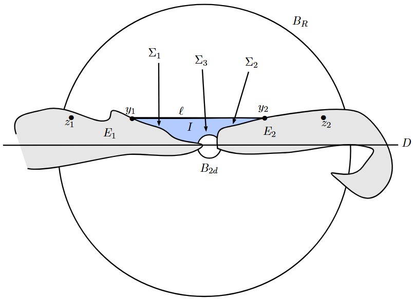
Since , the following two points exist:
Let us denote by . If , the conclusion of the lemma holds true. We can assume that . In this case, , and , for . Thus there exist three curves , and such that the set is a curve that goes from to . By Lemma 5.7 below, we know that this curve may possibly have self-intersection points but only by a zero -measure set.
The height bound (Lemma 6.1) gives
Thus, by the triangle inequality and the previous one, we get
| (89) |
At this point we use the -minimality relation to estimate the right-hand side of (5.3). We denote by the interior of the Jordan curve . By the -minimality of with respect to , we get
The inequality can be simplified as
By adding to both sides of the previous inequality, we infer that
Combining (5.3) with the previous inequality and using the Ahlfors regularity, we obtain
| (90) | ||||
| (91) | ||||
| (92) | ||||
| (93) |
The conclusion of the lemma follows by applying Lemma 5.6 below. ∎
Lemma 5.6.
Let a given set such that and satisfying the following property: there exists such that for all ,
where is the diameter of parallel to . Then, up to a rotation,
Proof.
Let . For any point we denote by the the diameter of parallel to . From our assumption on we know that for all it holds,
In particular, and since , this implies that the angle between and the direction of is small. More precisely, if is a unit vector in the direction of , then
and, accordingly,
| (94) |
Let be the angle between the vectors and , in such a way that . Then we deduce from (94) that
In other words, all the diameters , for , must be contained in an angular sector of aperture at most around . By assuming that , the first vector of the canonical basis of , we conclude that, for all , and finally, for all , The proposition follows from the elementary inequality, , which valid for all . ∎
We are now ready to proof the main result of this section and of the paper.
Proof of Theorem 1.2.
We may assume by contradiction that for every and there exist two connected components of such that
Let . By Lemma 5.5, there exist a ball and two connected components and of and such that they are contained in a rectangle. More precisely, up to a rotation,
with , with depending on the Ahlfors regularity constant. Without loss of generality, we may assume that .
Next, we want to find a curve which is lower Ahlfors-regular. The easiest way to do so is to find a connected subset of whose diameter is comparable to the diameter of . For that purpose, we use the following general topological result, which follows directly from the main theorem of [10] (see also [27, Theorem 14.2 p. 123]): if is an open set such that is connected, then is connected. To simplify the notation, we denote for a moment by the connected component . In particular we know that . Let be the connected component of containing the point . Then , where is the collection of all the other connected components of different from . In particular, is a closed set, for any . Applying Lemma 6.2 we deduce that is connected. Therefore, from [10] we know that is connected. Furthermore, it is easy to see that . Let us further show that
| (95) |
Indeed, from Lemma 5.5 we know that contains a point satisfying , and . Since is open and connected, it is pathwise connected. There exists a curve inside from the point to a point on . This curves stays inside the rectangle . By consequence, each vertical line must intersect for all , and (95) follows. We then define (see Figure 2.).
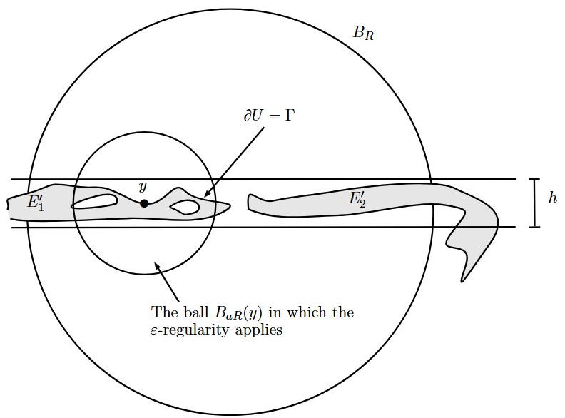
Since is connected, it satisfies the following lower Ahlfors regularity property:
Then by Lemma 4.4 there exist two constants , and a ball such that
for sufficiently small. By -regularity we have that is a -hypersurface. We can choose and so that the radius of the ball is greater than the height of the rectangle, that is . Indeed,
which concludes the proof. Indeed, this is clearly a contradiction with the fact that was supposed to be totally contained in the rectangle. ∎
The following lemma has been used in the proof of Lemma 5.5 and it holds when . It states that, under some mild regularity assumptions on a set , the boundaries of connected components cannot touch by a positive -measure set.
Lemma 5.7.
Let be a set of finite perimeter satisfying a lower Ahlfors-regularity inequality and such that
| (96) |
Let and be two connected components of and let . Then does not belong to . As a consequence,
Proof.
Assume by contradiction that . We know that admits an approximative tangent plane at point . From (96) we deduce that is actually an approximative tangent plane for as well. Then since satisfies a lower Ahlfors-regularity inequality, it is classical to see that this approximative tangent plane is actually a true tangent plane. Let us write more details about this last fact.
We assume without loss of generality that and let be fixed. Since is an approximative tangent plane we know that
| (97) |
Now we claim that there exists such that, for all ,
Otherwise, if , since is lower Ahlfors regular then
Which would easily contradict (97) for small enough.
We may assume that for we can find such that for any we have
| (98) |
Without loss of generality we may assume that . We distinguish two cases.
Case 1: there exists such that
Let and . Let us define
Notice that if , then necessarily . Indeed, if is any other point, then the segment is contained in because is convex. Since belongs to the connected component , it holds that , thus proving . The same assertion holds for so that the following two alternatives must hold:
-
1.
and .
-
2.
and .
In both cases, it follows that there exists a positive constant such that
| (99) |
which is a contradiction if , being .
Case 2: for any it holds
We assume without loss of generality that . We take a point . Without loss of generality, we can assume that . Since is connected, and , we deduce that , for all . Let be a point in . Since , we know that .
Since , for all there exists a point such that . Let be a curve connecting and in , which exists because is a connected open set, thus arc-wise connected.
We define the vertical line
Since and meets interior points of for , we have that
Accordingly, by the coarea formula we get
for any . Moreover we know that for all ,
so that, all together,
which implies the following contradiction:
for .
∎
Remark 5.8.
The Lemma is false in higher dimensions: consider the -curve defined by
Then consider as being a very small open neighborhood of , with the property that and
Then we define , where . The two connected components of are and , for which their boundaries meet at the origin, which is a point that belongs to . However, we don’t know if the assertion still holds in higher dimensions for two connected components of a set of finite perimeter satisfying , and such that satisfies a lower Ahlfors-regularity inequality.
6 Appendix
The following lemma is a standard height bound which is taken from [4, Lemma 6.3] for the case of injective curves. Here we adapted the argument straightforwardly for a curve which is possibly non injective anymore, but for which the set of self-intersection points has zero measure.
Lemma 6.1.
Let be a curve with endpoints and , with image . We assume that is almost injective in the sense that, defining
it holds that . It follows that
| (100) |
Proof.
Let be a maximizer of the function , i.e., is the most distant point in from the segment , and define . Let us consider the point making an isosceles triangle with height . Denoting by and , according to Pythagoras Theorem, we have
Lemma 6.2.
Let be an open and connected set, and let be a family of closed connected sets such that for all . Then the set
is connected.
Proof.
Let us denote by
and assume that
where and are two disjoint open and connected subsets of . To prove that is connected, it is enough to prove that or . Let be fixed for a moment. Then, by assumption, but since is connected we deduce that or . Let us assume that . Let , which is assumed to be non empty. Since is open and , we actually infer that . But since , and since is connected, we conclude that . In other words we have proved that . Now for any other , arguing similarly we deduce that is also contained in one of the two open sets, that actually must be the same because is already known to be contained in . All in all we have proved that , as desired, and this achieves the proof. ∎
References
- [1] Luigi Ambrosio and Giuseppe Buttazzo. An optimal design problem with perimeter penalization. Calc. Var. Partial Differ. Equ., 1(1):55–69, 1993.
- [2] Luigi Ambrosio, Nicola Fusco, and Diego Pallara. Functions of bounded variation and free discontinuity problems. Oxford Math. Monogr. Oxford: Clarendon Press, 2000.
- [3] Adolfo Arroyo-Rabasa. Regularity for free interface variational problems in a general class of gradients. Calc. Var. Partial Differ. Equ., 55(6):44, 2016. Id/No 154.
- [4] Jean-François Babadjian, Flaviana Iurlano, and Antoine Lemenant. Partial regularity for the crack set minimizing the two-dimensional griffith energy. J. Eur. Math. Soc. (JEMS), 24(7):2443–2492, 2022.
- [5] Alexis Bonnet. On the regularity of the edge set of Mumford-Shah minimizers. In Variational methods for discontinuous structures. Applications to image segmentation, continuum mechanics, homogenization. Proceedings of the international conference, Como, Italy, September 8–10, 1994, pages 93–103. Basel: Birkhäuser, 1996.
- [6] Menita Carozza, Luca Esposito, and Lorenzo Lamberti. Quasiconvex bulk and surface energies: regularity. Adv. Nonlinear Anal., 13:34, 2024. Id/No 20240021.
- [7] Menita Carozza, Luca Esposito, and Lorenzo Lamberti. Quasiconvex bulk and surface energies with subquadratic growth. Math. Eng., 7:36, 2025.
- [8] Menita Carozza, Irene Fonseca, and Antonia Passarelli Di Napoli. Regularity results for an optimal design problem with a volume constraint. ESAIM, Control Optim. Calc. Var., 20(2):460–487, 2014.
- [9] Menita Carozza, Irene Fonseca, and Antonia Passarelli di Napoli. Regularity results for an optimal design problem with quasiconvex bulk energies. Calc. Var. Partial Differ. Equ., 57(2):34, 2018. Id/No 68.
- [10] Andrzej Czarnecki, Marcin Kulczycki, and Wojciech Lubawski. On the connectedness of boundary and complement for domains. Annales Polonici Mathematici, 103, 01 2012.
- [11] Guy David. Singular sets of minimizers for the Mumford-Shah functional, volume 233 of Prog. Math. Basel: Birkhäuser, 2005.
- [12] Guy David and Stephen Semmes. Analysis of and on uniformly rectifiable sets, volume 38 of Math. Surv. Monogr. Providence, RI: American Mathematical Society, 1993.
- [13] Guy David and Stephen Semmes. Quantitative rectifiability and Lipschitz mappings. Trans. Am. Math. Soc., 337(2):855–889, 1993.
- [14] Guido De Philippis and Alessio Figalli. A note on the dimension of the singular set in free interface problems. Differ. Integral Equ., 28(5-6):523–536, 2015.
- [15] Luca Esposito. Density lower bound estimate for local minimizer of free interface problem with volume constraint. Ric. Mat., 68(2):359–373, 2019.
- [16] Luca Esposito and Nicola Fusco. A remark on a free interface problem with volume constraint. J. Convex Anal., 18(2):417–426, 2011.
- [17] Luca Esposito and Lorenzo Lamberti. Regularity results for a free interface problem with Hölder coefficients. Calc. Var. Partial Differ. Equ., 62(5):49, 2023. Id/No 156.
- [18] Luca Esposito and Lorenzo Lamberti. Regularity results for an optimal design problem with lower order terms. Adv. Calc. Var., 16(4):1093–1122, 2023.
- [19] Luca Esposito, Lorenzo Lamberti, and Giovanni Pisante. Regularity results for almost-minimizers of anisotropic free interface problem with Hölder dependence on the position. Preprint, arXiv:2404.02086 [math.OC] (2024), 2024.
- [20] Nicola Fusco and Vesa Julin. On the regularity of critical and minimal sets of a free interface problem. Interfaces Free Bound., 17(1):117–142, 2015.
- [21] Lorenzo Lamberti. A regularity result for minimal configurations of a free interface problem. Boll. Unione Mat. Ital., 14(3):521–539, 2021.
- [22] Christopher J. Larsen. Distance between components in optimal design problems with perimeter penalization. Ann. Sc. Norm. Super. Pisa, Cl. Sci., IV. Ser., 28(4):641–649, 1999.
- [23] Christopher J. Larsen. Regularity of components in optimal design problems with perimeter penalization. Calc. Var. Partial Differ. Equ., 16(1):17–29, 2003.
- [24] F. H. Lin and R. V. Kohn. Partial regularity for optimal design problems involving both bulk and surface energies. Chinese Annals of Mathematics, 20(2):137–158, 1999.
- [25] Fang Hua Lin. Variational problems with free interfaces. Calc. Var. Partial Differ. Equ., 1(2):149–168, 1993.
- [26] Francesco Maggi. Sets of finite perimeter and geometric variational problems. An introduction to geometric measure theory, volume 135 of Camb. Stud. Adv. Math. Cambridge: Cambridge University Press, 2012.
- [27] M. H. A. Newman. Elements of the topology of plane sets of points. New York, NY: Dover Publications, reprint of the 2nd ed. edition, 1992.
- [28] Séverine Rigot. Big pieces of -graphs for minimizers of the Mumford-Shah functional. Ann. Scuola Norm. Sup. Pisa Cl. Sci. (4), 29(2):329–349, 2000.
- [29] Italo Tamanini. Regularity results for almost minimal oriented hypersurfaces in . Lecce: Dipartimento di Matematica dell’Università di Lecce, 1984.