Model-independent cosmological inference after the DESI DR2 data with improved inverse distance ladder
Abstract
Recently, the baryon acoustic oscillations (BAO) measurements from the DESI survey have suggested hints of dynamical dark energy, challenging the standard CDM model. In this work, we adopt an improved inverse distance ladder approach based on the latest cosmological data to provide a model-independent perspective, employing a global parametrization based on cosmic age (PAge). Our analysis incorporates DESI DR2 BAO measurements, cosmic chronometer (CC) data, and type Ia supernovae (SNe) observations from either the DESY5 or PantheonPlus datasets. For the DESY5+DESI DR2+CC datasets, we obtain . This value is consistent with the Planck 2018 result, while shows tension with the SH0ES measurement. Furthermore, by mapping specific cosmological models into PAge approximation parameter space , our model-independent analysis reveals a notable deviation from the model, as indicated by the DESY5 and DESI DR2 datasets. Finally, DESY5+DESI DR2+CC datasets provide nearly decisive evidence favoring the PAge model over the standard model. These findings highlight the need for further investigation into the expansion history to better understand the deviations from the model.
I INTRODUCTION
The simplest cold dark matter () model has been remarkably consistent with most astronomical observations across different epochs and scales of the universe Riess et al. (1998); Perlmutter et al. (1999); Brout et al. (2022); Asgari et al. (2021); Troxel et al. (2018); Aiola et al. (2020). However, the persistent discrepancy in the value of the Hubble constant inferred from the early and late universe, known as the Hubble tension, is challenging the model Di Valentino et al. (2021a); Perivolaropoulos and Skara (2022); Shah et al. (2021); Verde et al. (2019). Among various discrepancies, the most significant is the over divergence between the Planck 2018 estimate of , indirectly inferred from the cosmic microwave background (CMB) data assuming the model Aghanim et al. (2020), and the SH0ES result of directly measured from the type Ia supernovae (SNe) calibrated using the Cepheid variables Riess et al. (2022). The tension cannot be merely explained by a statistical fluctuation, even after the reanalysis of systematic uncertainties Akrami et al. (2020); Zhang et al. (2017a). Therefore, the irreconcilable tension may indicate underlying systematics or new physics beyond Di Valentino et al. (2021b); Bernal et al. (2016); Abdalla et al. (2022).
However, no consensus has yet been reached on resolving the tension based on current data. Given this discrepancy between the early and late universe, proposed scenarios can broadly be classified into early-time or late-time solutions.
In early-time solutions, new physics is introduced to reduce the sound horizon, , thereby increasing while preserving the baryon acoustic oscillation (BAO) measurement of . One realization involves modifying expansion history by introducing additional energy components around the epoch of matter-radiation equality, such as early dark energy Poulin et al. (2019); Karwal and Kamionkowski (2016); Mörtsell and Dhawan (2018); Kamionkowski et al. (2014); Berghaus and Karwal (2020) or extra neutrino species Zhang et al. (2015); Zhao et al. (2017a, b); Feng et al. (2020); Kreisch et al. (2020); Wyman et al. (2014); Sakstein and Trodden (2020). Alternatively, early-time solutions may also involve modifying the recombination history Sekiguchi and Takahashi (2021); Chiang and Slosar (2018); Mirpoorian et al. (2024) or introducing primordial magnetic fields Jedamzik and Pogosian (2020); Jedamzik et al. (2025); Jedamzik and Abel (2013). However, these early-time solutions are in tension with other cosmological observables, such as the fluctuation amplitude and the integrated Sachs-Wolfe effect, as discussed in the no-go arguments of Refs. Hill et al. (2020); Krishnan et al. (2020); Jedamzik et al. (2021); Vagnozzi (2023); Dutta et al. (2019). Late-time solutions modify the Hubble parameter in the late universe, so that it can accommodate the SH0ES result locally while leaving the CMB anisotropy spectrum unchanged, such as the deformation of the dark-energy equation of state Wang et al. (2016); Agrawal et al. (2023); Li and Shafieloo (2019); Li (2004); Shapiro and Sola (2002), modified gravity Aluri et al. (2023); Capozziello and De Laurentis (2011); De Felice and Tsujikawa (2010), parameter transitions in the late universe Mortonson et al. (2009); Kazantzidis and Perivolaropoulos (2019). Analogous to early-time solutions, various no-go arguments have also been raised against the late-time scenarios. The requirement of consistency between low redshift cosmological distance measurements from BAO and SNe imposes strong constraints on the late-time solutions Benevento et al. (2020); Yang et al. (2021). Moreover, these solutions cannot reconcile the tension and tension simultaneously, as Refs. Guo et al. (2019); Gao et al. (2021); Heisenberg et al. (2022); Dutta et al. (2019); Alestas and Perivolaropoulos (2021) pointed out.
In light of the plethora of proposed cosmological models and corresponding no-go arguments, it is compelling to explore new and independent measurements of . For instance, techniques such as strong gravitational lensing time delay Birrer et al. (2019); Shajib et al. (2020) and gravitational wave standard sirens Guidorzi et al. (2017); Song et al. (2025) provide an independent perspective on this tension. We can also employ other independent calibrators to replace Cepheid variables in the distance ladder, such as megamasers Pesce et al. (2020), the tip of the red giant branch Freedman (2021), surface brightness fluctuations Blakeslee et al. (2021), Mira variables Huang et al. (2019).
The inverse distance ladder (IDL) calibrates the SNe via anchored BAO instead of Cepheid variables, providing a model-insensitive method to infer Aubourg et al. (2015); Cuesta et al. (2015); Verde et al. (2017); Lemos et al. (2019). In the traditional IDL, the BAO data are anchored using an prior derived from the CMB or big bang nucleosynthesis. Then the data are used to calibrate SNe to give an absolute distance. Finally, the distance is extrapolated to to infer under a fiducial model Percival et al. (2010); Heavens et al. (2014); Abbott et al. (2018); Alam et al. (2021); Camilleri et al. (2025); Adame et al. (2025); Macaulay et al. (2019).
It should be noted that the prior introduces dependence on early-universe physics Aylor et al. (2019). The effect of this prior has been systematically evaluated in Refs. Barua and Desai (2024); Luongo and Muccino (2024). To mitigate such dependence, the prior can be replaced with other independent measurements. Cosmic chronometer (CC) measure directly, rather than through integrals of , such as those involved in lensing distances from strong lensing systems Wojtak and Agnello (2019); Taubenberger et al. (2019); Wang et al. (2022); Gong et al. (2024), thus offering higher sensitivity to cosmological parameters Moresco (2024); Vagnozzi et al. (2022); Jimenez et al. (2019). CC data have been widely applied as an effective replacement for in constructing IDL Guo et al. (2025); Luongo and Muccino (2024); Favale et al. (2023); Cai et al. (2022a).
Furthermore, adopting a fiducial model will inevitably introduce model dependence. To avoid this, the traditional approach is to parameterize via a Taylor expansion in terms of or , known as the cosmography method Camilleri et al. (2025); Pourojaghi et al. (2025); Luongo and Muccino (2024); Lemos et al. (2019); Cattoen and Visser (2007); Zhang et al. (2017b); Chiba and Nakamura (1998); Capozziello et al. (2011); Aviles et al. (2012). Alternatively, purely data-driven techniques such as Gaussian Process (GP) have been employed to reconstruct Guo et al. (2025); Jiang et al. (2024); He et al. (2022); Mukherjee and Sen (2024); Yang et al. (2023). However, both approaches possess intrinsic limitations. The Taylor expansion is problematic at Banerjee et al. (2021); Cai et al. (2022a, b); Zhang et al. (2017b). GP methods are sensitive to the choice of kernel functions and tend to yield smaller errors at the cost of strongly correlated results Ó Colgáin and Sheikh-Jabbari (2021); Kjerrgren and Mortsell (2022). To address these limitations and achieve a fully model-independent method, we adopt a global parametrization based on the cosmic age (PAge) model Huang (2020); Luo et al. (2020) to accurately reproduce late-time cosmological behavior across a wide redshift range.
The PAge model can be interpreted as an effective description of homogeneous late-time scenarios. Moreover, for models where the evolves rapidly, a Taylor expansion in terms of or requires high-order terms to accurately capture the behavior. However, since the cosmic age is defined through the integral of , it evolves more smoothly. As a result, even pronounced changes in can typically be captured by a low-order expansion in . So the PAge model has been employed as a substitute for specific physical models to mitigate model dependence. The studies Huang et al. (2021a, 2022); Li et al. (2022) have employed the PAge model to analyze gamma-ray bursts, redshift-space distortions and quasars. Refs. Cai et al. (2022a, b); Huang et al. (2025a) have derived no-go theorems against late-time solutions through the comparison between the PAge (denoted as late-time scenarios) and models.
Recently, the Dark Energy Spectroscopic Instrument (DESI) collaboration reported a hint of dynamical dark energy in the first data release (DR1), which was further increased to in the second data release (DR2) Adame et al. (2025); Abdul Karim et al. (2025). This finding has sparked intense discussions about possible new physics and systematic uncertainties Pourojaghi et al. (2024); Colgáin and Sheikh-Jabbari (2024); Jia et al. (2025); Wang et al. (2024a); Huang et al. (2025b); Cortês and Liddle (2024); Efstathiou (2024); Abreu and Turner (2025); Pang et al. (2024); Fikri et al. (2024); Feng et al. (2025); Du et al. (2025a); Li et al. (2024a, b, 2025); Du et al. (2025b); Pang et al. (2025); Wang and Piao (2025, 2024); Lodha et al. (2025); Pan et al. (2025); You et al. (2025); Pan and Ye (2025); Silva et al. (2025). This behavior, which deviates from can be effectively described by the PAge model. This motivates us to propose a PAge-improved IDL to yield fully model-independent cosmological constraints in this work. Our results will provide model-independent perspectives on the tension and the hint of dynamical dark energy.
II METHODOLOGY
II.1 The PAge model
In IDL, a fiducial model is needed to trace the universal expansion history back to to determine . To achieve a model-independent analysis of late-time data, the simplest technique is a Taylor expansion Visser (2004); Cattoen and Visser (2007) about redshift Zhang et al. (2017b); Chiba and Nakamura (1998) or y-redshift, Capozziello et al. (2011); Aviles et al. (2012). However, both ways become problematic at due to the deviation from the target model, as discussed in Refs. Hu and Wang (2022); Cai et al. (2022a).
The PAge model is introduced to provide a global approximation of with the cosmic age Huang (2020). It remains consistent with the target model at high redshift and is more precise than - or -expansion. Actually, it is a calibrated Taylor expansion around . Motivated by the fact that the product of the Hubble constant and current age of the universe differs little among most cosmological models Vagnozzi et al. (2022), we begin by expanding about the current cosmic age as Wang et al. (2024b)
| (1) |
Neglecting the brief radiation-dominated era, matter domination in the early universe requires Eq. (1) to satisfy the following condition
| (2) |
which introduces a calibration to Taylor expansion to prevent it from diverging at high redshift. Moreover, for simplicity and Occam’s razor, we only expand to the quadratic order. The higher-order terms have been proven to be unnecessary given the accuracy level of current data in Refs. Cai et al. (2022b); Huang et al. (2021b). Thus, the final calibrated expansion takes the following form
| (3) |
where two free parameters and are introduced to calibrate the expansion to satisfy Eq. (2). Their exact forms can be derived by combining the quadratic expansion of Eq. (1) with the constraint condition Eq. (2),
| (4) |
The deceleration parameter appears in Eq. (4) arising from the quadratic term of Eq. (1). It is clear that and quantify the extent to which the real universe deviates from the matter-dominated era relation in Eq. (3). To obtain , we can replace in Eq. (3) with its definition , and integrate both sides,
| (5) |
Again, in Eq. (5), and quantify the deviation from the matter-dominated universe .
The PAge model, as a type of Taylor expansion, can map specific dark energy models into a two-parameter space . Thus, the deviation from the model is clearly illustrated in the parameter space. For simplicity, the mapping procedure is carried out by equating the deceleration parameter between the PAge model and the specific cosmological model, followed by computing for the reference model. Subsequently, can be derived from Eq. (4). More details about model mapping are provided in Ref. Luo et al. (2020).
In the following, we explicitly demonstrate how to map the specific dark energy models discussed in this paper into , including , , .
For with when mapped to the PAge model, the deceleration parameter is
| (6) |
and reads
| (7) |
The model can be mapped in the same manner as
| (8) |
and the corresponding takes
| (9) |
Setting and , the results are applicable to the model.
II.2 Cosmological datasets
In this section, we present an overview of various combinations of cosmological data used to construct the IDL, including SNe data from PantheonPlus and DESY5, BAO measurements from DESI DR2 and Sloan Digital Sky Survey (SDSS), and CC data.
-
•
SNe: SNe are known as the standard candles due to their uniform intrinsic luminosity. The SNe data records the apparent magnitude . The luminosity distance can be derived from the magnitude–redshift relation
(10) where is the absolute magnitude of SNe. is the intercept of the magnitude–redshift relation Eq. (10). It is evident that and are degenerate in , making it impossible to constrain both and with SNe data alone. In IDL, we incorporate BAO and CC (described below) to break this degeneracy, avoiding the dependence on external prior.
The chi-squared statistic for SNe is defined as follows
(11) where is the distance moduli residual vector. Distance modulus is defined as . denotes the inverse combined statistical and systematic covariance matrix of the SNe sample.
We use two different SNe datasets, including PantheonPlus111PantheonPlus data available at https://github.com/PantheonPlusSH0ES/DataRelease and DESY5222DESY5 data available at https://github.com/des-science/DES-SN5YR.
The PantheonPlus SNe compilation consists of 1701 light curves of 1550 spectroscopically confirmed SNe Ia in the redshift range Scolnic et al. (2022). To reduce the effect of strong peculiar velocity dependence at low redshift Brout et al. (2022), only 1550 data points in the range are used.
The DESY5 SNe sample is the largest and deepest single sample survey to date consisting of 1635 SNe Ia Abbott et al. (2024); Vincenzi et al. (2024); Sánchez et al. (2024) distributed in complemented by 194 low-redshift SNe Ia spanning Hicken et al. (2009, 2012); Krisciunas et al. (2017); Foley et al. (2018). The DESY5 data provide the Hubble diagram redshift, corrected apparent magnitudes , distance moduli and the corresponding distance moduli errors and related quantities. Since the distance moduli contain no information about , we follow Refs. Huang et al. (2025b); Camilleri et al. (2025) to use the corrected apparent magnitudes to construct the distance moduli residual as to constrain .
-
•
BAO: The BAO records the imprint of early-universe plasma fluctuations in the late-time large-scale structure. BAO data provide three types of distances with respect to a fiducial cosmology, measured along different directions. Along the line-of-sight direction, BAO measures the Hubble distance
(12) and along the transverse direction, BAO measures the (comoving) angular diameter distance
(13) Taking the spherical average of both directions, BAO measures
(14) where is treated as a free parameter in our analysis to eliminate the model dependence introduced by the prior in traditional IDL.
The chi-squared statistic for BAO takes
(15) where denotes the residual vector between the BAO data and the corresponding model values. is the inverse covariance matrix of the BAO data.
Two BAO datasets from DESI333DESI DR2 data available at https://github.com/CobayaSampler/bao_data/tree/master/desi_bao_dr2. and SDSS444SDSS data available at https://svn.sdss.org/public/data/eboss/DR16cosmo/tags/v1_0_0/likelihoods/BAO-plus/ are used to delve into the role that BAO plays in the cosmological constraint, and these datasets are listed in Table 1.
We adopt the DESI DR2 BAO measurements which include extracted from large scale structure traces across multiple distinct redshift bins Abdul Karim et al. (2025).
The SDSS BAO data are employed in this paper to cross-check our findings and connect with the existing literature. It includes two low-redshift data points 6dFGS Beutler et al. (2011), SDSS DR7 MGS Ross et al. (2015) and SDSS DR16 data Alam et al. (2021).
Table 1: The BAO samples utilized in this work including DESI DR2 data and SDSS data. Tracer DESI DR2 BGS 0.30 - - 7.94 0.08 LRG1 0.51 13.59 0.17 21.86 0.43 - LRG2 0.71 17.35 0.18 19.46 0.33 - LRG3 + ELG1 0.93 21.58 0.15 17.64 0.19 - ELG2 1.32 27.60 0.32 14.18 0.22 - QSO 1.48 30.51 0.76 12.82 0.52 - Ly 2.33 38.99 0.94 8.63 0.10 - SDSS 6dFGS 0.106 - - 0.336 0.015 MGS 0.15 - - 4.47 0.17 LRG 0.70 17.86 0.33 19.33 0.53 - ELG 0.85 - - QS0 1.48 30.69 0.80 13.26 0.55 - Ly 2.33 37.6 1.9 8.93 0.28 - Ly QSO 2.33 37.3 1.7 9.08 0.34 - Table 2: 32 CC data points with error. Reference 0.09 69 12 Jimenez et al. (2003) 0.17 83 8 Simon et al. (2005) 0.27 77 14 Simon et al. (2005) 0.4 95 17 Simon et al. (2005) 0.9 117 23 Simon et al. (2005) 1.3 168 17 Simon et al. (2005) 1.43 177 18 Simon et al. (2005) 1.53 140 14 Simon et al. (2005) 1.75 202 40 Simon et al. (2005) 0.48 97 62 Stern et al. (2010) 0.88 90 40 Stern et al. (2010) 0.1791 75 4 Moresco et al. (2012) 0.1993 75 5 Moresco et al. (2012) 0.3519 83 14 Moresco et al. (2012) 0.5929 104 13 Moresco et al. (2012) 0.6797 92 8 Moresco et al. (2012) 0.7812 105 12 Moresco et al. (2012) 0.8754 125 17 Moresco et al. (2012) 1.037 154 20 Moresco et al. (2012) 0.07 69 19.6 Zhang et al. (2014) 0.12 68.6 26.2 Zhang et al. (2014) 0.2 72.9 29.6 Zhang et al. (2014) 0.28 88.8 36.6 Zhang et al. (2014) 1.363 160 36.6 Moresco (2015) 1.965 186.5 50.4 Moresco (2015) 0.3802 83 13.5 Moresco et al. (2016) 0.4004 77 10.2 Moresco et al. (2016) 0.4247 87.1 11.2 Moresco et al. (2016) 0.4497 92.8 12.9 Moresco et al. (2016) 0.4783 80.9 9 Moresco et al. (2016) 0.47 89 49.6 Ratsimbazafy et al. (2017) 0.80 113.1 28.5 Jiao et al. (2023) -
•
CC: CC measurements are incorporated to break the and degeneracy in BAO data, serving a role analogous to the prior in traditional IDL. It directly measures the Hubble parameter through massive passively evolving galaxies with old stellar populations and very low star formation rates Moresco (2023). By comparing two galaxies formed at the same time but separated by a small redshift interval, the Hubble parameter can be calculated using the differential age method Jimenez and Loeb (2002), without assuming any cosmological model,
(16) where is the derivative of redshift with respect to the look-back time. Its nature as a direct measurement of makes it highly sensitive to cosmological parameters.
As CC data are not entirely independent, we incorporate correlations through the use of a covariance matrix when available. We adopt 32 CC data points, listed in Table 2, including 15 correlated measurements with the corresponding covariance matrix compiled in Ref. Moresco et al. (2020), and 17 uncorrelated ones. For the correlated measurements, we adopt the covariance matrix as described in Refs. Moresco et al. (2020, 2022),
(17) where represents the diagonal covariance matrix containing statistical uncertainties, accounts for systematic effects, including those from stellar population models, metallicity assumptions, and potential contamination from residual young stellar components.
In this work, we adopt the recommended covariance matrix combination from Moresco (2021),
(18) where denotes the contribution from uncertainties in stellar metallicity estimates. accounts for uncertainties arising from the odd one out stellar population synthesis (SPS) model. reflects uncertainties due to the adopted initial mass function (IMF). For a detailed discussion of CC data, we refer the reader to Ref. Moresco et al. (2020).
For data points not discussed in Ref. Moresco et al. (2020), only the diagonal components are considered. The final is
(19) where are the diagonal components mentioned above, and is the residual vector between the CC data and the model values.
We consider four datasets, namely DESY5 + DESI DR2 + CC, DESY5 + SDSS + CC, PantheonPlus + DESI DR2 + CC, PantheonPlus + SDSS + CC. The final combined likelihood, , is used to constrain the PAge model with five free parameters . Then we employ the Markov Chain Monte Carlo (MCMC) sampler emcee555https://github.com/dfm/emcee Foreman-Mackey et al. (2013) to explore the parameter space and obtain best-fit parameters through minimization. For comparison, we also consider the model, with four free parameters . Uniform priors are adopted for the following parameter ranges . Posterior samples are analyzed and visualized using GetDist666https://github.com/cmbant/getdist Lewis (2019). For model comparison, we use the MCEvidence777https://github.com/yabebalFantaye/MCEvidence algorithm as described in Ref. Heavens et al. (2017) to compute the Bayesian evidence directly from the MCMC chain.
| Dataset | ||||||
| PAge | ||||||
| DESY5+DESI DR2+CC | 0.23 0.04 | 0.94 0.01 | – | -19.36 0.07 | 67.91 2.33 | 145.05 4.88 |
| DESY5+SDSS+CC | 0.16 0.06 | 0.95 0.01 | – | -19.35 0.07 | 67.74 2.36 | 143.47 4.99 |
| PantheonPlus+DESI DR2+CC | 0.31 0.06 | 0.96 0.01 | – | -19.38 0.07 | 68.97 2.42 | 144.97 4.89 |
| PantheonPlus+SDSS+CC | 0.25 0.07 | 0.96 0.02 | – | -19.39 0.08 | 68.58 2.49 | 143.35 4.99 |
| DESY5+DESI DR2+CC | – | – | 0.32 0.01 | -19.35 0.07 | 68.99 2.35 | 145.18 4.89 |
| DESY5+SDSS+CC | – | – | 0.35 0.01 | -19.38 0.07 | 67.46 2.37 | 143.42 4.99 |
| PantheonPlus+DESI DR2+CC | – | – | 0.30 0.01 | -19.37 0.07 | 69.75 2.39 | 144.98 4.89 |
| PantheonPlus+SDSS+CC | – | – | 0.32 0.02 | -19.39 0.08 | 69.08 2.51 | 143.16 4.99 |
III RESULTS AND DISCUSSION
Our primary goal is to derive a model-independent estimate of , as well as other cosmological parameters and , using the PAge-improved IDL. The summary of the full cosmological results is presented in Table 3, along with the corresponding result for comparison. The one- and two-dimensional posterior distributions of the cosmological parameters in the PAge model are presented in Fig. 1. For the DESY5+DESI DR2+CC datasets, the PAge model yields
| (20) |
at the confidence level (C.L.). Our estimate agrees with the Planck 2018 result of Aghanim et al. (2020). However, a mild tension persists at the level in comparison with the local SH0ES measurement of Riess et al. (2022). Other datasets exhibit the same agreement with the Planck result and a similar tension level with the SH0ES measurements. Specifically, DESY5+SDSS+CC datasets show a discrepancy, while PantheonPlus+DESI DR2+CC and PantheonPlus+SDSS+CC datasets exhibit and discrepancies, respectively. Our results show larger uncertainty than other traditional IDLs Camilleri et al. (2025); Aubourg et al. (2015); Macaulay et al. (2019) due to the substitution of the Gaussian prior with the more uncertain CC measurements.
Notably, the DESY5 data yield a lower and a higher compared to the PantheonPlus data, which tends to enlarge the tension. This trend is consistent with previous findings reported in Refs. Colgáin and Sheikh-Jabbari (2024); Notari et al. (2024); Adame et al. (2025). A shift in is observed between the DESI DR2 and SDSS BAO datasets, across both supernova samples. This behavior is expected within the IDL framework, where the CC data serve to anchor the BAO measurements and infer the , rather than relying on a prior . DESI DR2 data yield a higher than SDSS data by approximately .
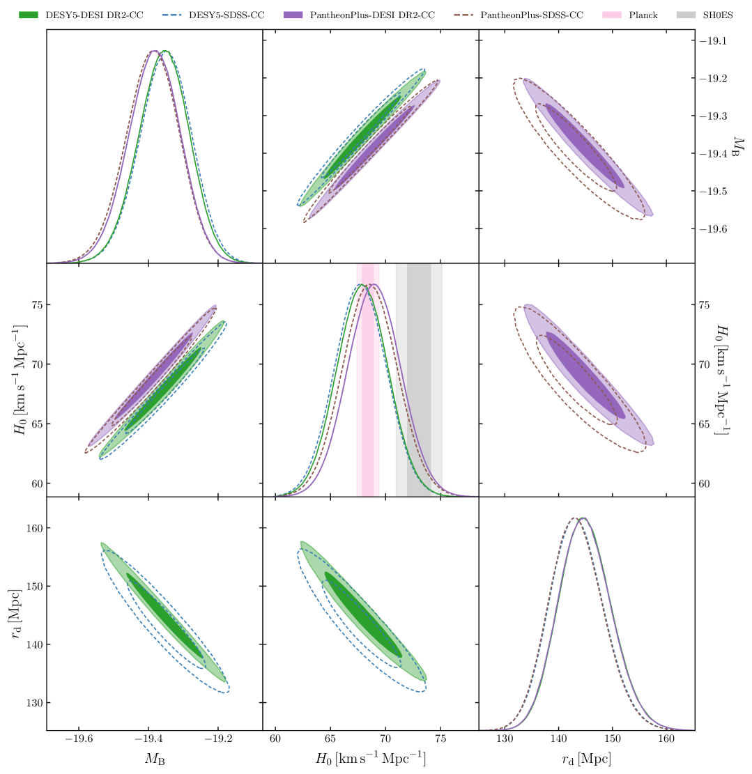
The tension reported in Refs. Huang et al. (2025b, a) is likewise observed in our analysis. This manifests as a shift in the intercept of the magnitude–redshift relation in the – parameter space, as illustrated in Fig. 1. It has been argued that this effect may originate from the low-redshift supernovae in DESY5 data Huang et al. (2025b).
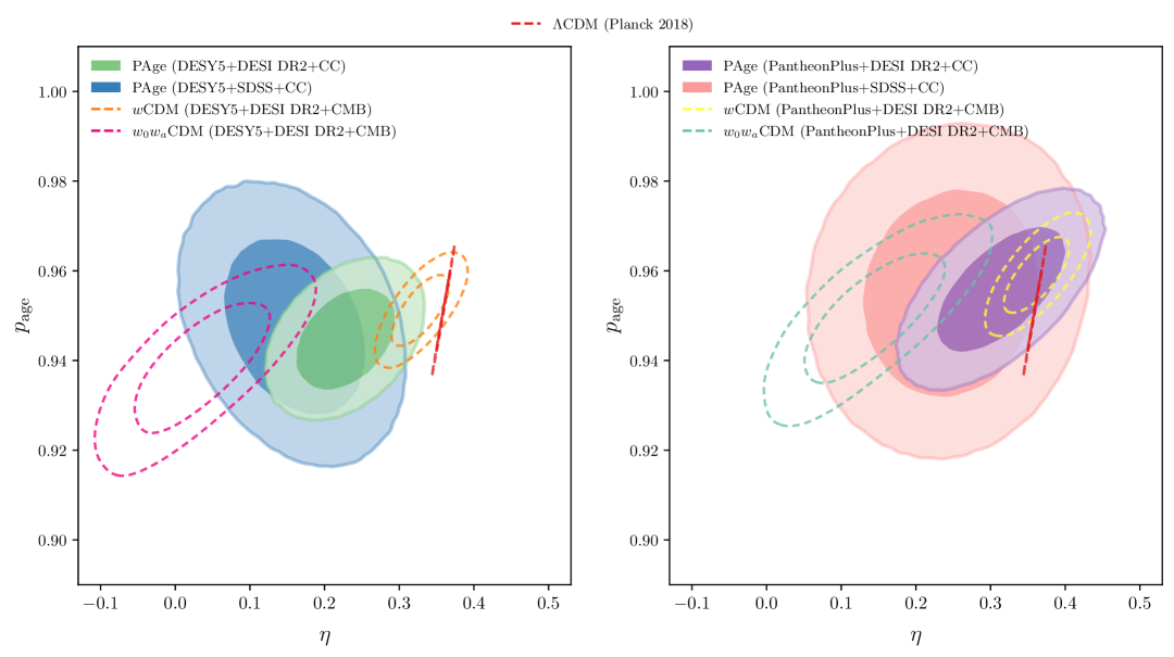
After examining how the choice of SNe and BAO datasets influences the cosmological parameters, we now focus on the approximation parameters of the PAge model itself, namely and . These two parameters play a central role in offering insights into potential late-time modifications to cosmic expansion. The posterior distributions in the plane for the four datasets are shown in Fig. 2. For comparison, previous results from Aghanim et al. (2020) and DESI DR2 Abdul Karim et al. (2025) are mapped into the PAge model. The mapping procedure is detailed in Eqs. (4), (6), (7), (8), and (9). Note that the PAge model contains one additional parameter compared to , which causes the mapped region of in the space to appear as a line. We adopt the DESI DR2 results for and models Abdul Karim et al. (2025). As shown in Fig. 2, it is evident that our results deviate from the model, showing a lower value of for the DESY5 dataset. In contrast, for the PantheonPlus samples, different BAO combinations remain consistent with .
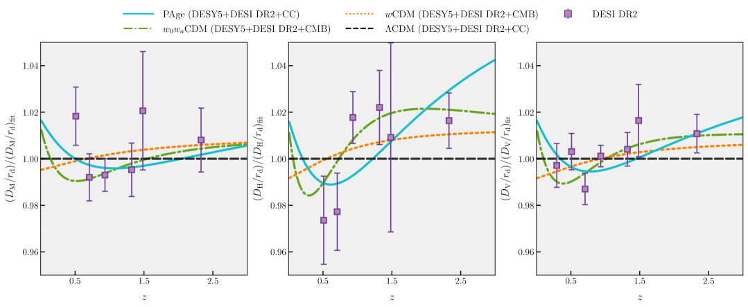
To better understand these results, we reconstruct the BAO distance predicted by the PAge, and in Fig. 3, based on our best-fit model in the DESY5+DESI DR2+CC datasets. The PAge model exhibits a distinctive trend driven by the DESI DR2 data. In comparison to the model, it predicts slightly enhanced BAO distances at very low redshifts, suppressed distances at intermediate redshifts, and elevated values again at high redshifts across all configurations. While the model attempts to capture this behavior, it fails to reproduce the variation across the relevant redshift range. In contrast, the model, which incorporates dynamically evolving equation of state, is more capable of reproducing this characteristic trend.
These findings suggest that the DESI DR2 data may not be fully compatible with the model, which lack the flexibility to capture such rapid variations in the expansion history, thereby hinting at a preference for dynamical dark energy. It is important to emphasize that the PAge model is essentially a calibrated Taylor expansion, and therefore independent of any specific cosmological model. As such, our results serve as a model-agnostic indication of the underlying behavior of the universe. The presence of this trend in our findings suggests that any viable theoretical model must be capable of reproducing this trend to be consistent with the data.
To quantitatively evaluate the performance of the PAge model relative to the model, we perform Bayesian inference across different datasets. Specifically, the Bayes factors are calculated in logarithmic space,
| (21) |
where and are Bayesian evidence of PAge and models, respectively. The Bayesian evidence is defined as
| (22) |
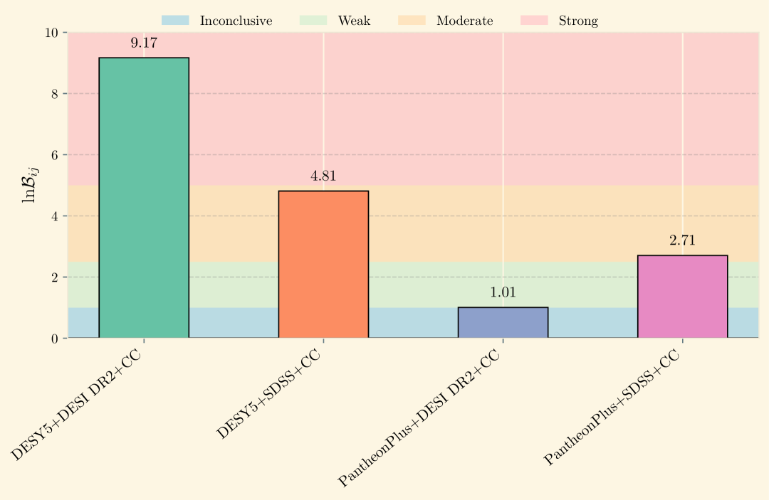
where is the likelihood of the data given the parameters and model , is the prior probability of under , and is the prior of . The extent of model preference is assessed using the Jeffreys’ scale, as described in Ref. Trotta (2008).
-
•
, inconclusive evidence.
-
•
, weak evidence.
-
•
, moderate evidence.
-
•
, strong evidence.
-
•
, decisive evidence.
In Fig. 4, we present the final model comparison results, with the PAge model assessed relative to the fiducial across four datasets. Positive values indicate a preference for the PAge model, while negative values indicate a preference for the model. Specifically, we find for DESY5+DESI DR2+CC, DESY5+SDSS+CC, PantheonPlus+DESI DR2+CC, and PantheonPlus+SDSS+CC, respectively. It is clear that the PAge model consistently provides a better fit than the standard across all datasets. In particular, for the DESY5+DESI DR2+CC datasets, the Bayes factor is 9.17, indicating nearly decisive evidence in favor of the PAge model over the model.
IV CONCLUSION
The tension between the early-universe and late-universe measurements of has become one of the most significant challenges in modern cosmology. Recently, DESI DR1 Adame et al. (2025) and DR2 Abdul Karim et al. (2025) have further sharpened this tension with addition hints of dynamical dark energy in and level. In the context of the tension, numerous theoretical models have been proposed, although many models face corresponding no-go arguments. Similarly, the hint of dynamical dark energy has been critically examined through the reanalyzes of the DESY5 SNe data Huang et al. (2025b); Efstathiou (2024); Vincenzi et al. (2025); Gialamas et al. (2025) and the DESI BAO measurements Zheng et al. (2024); Mukherjee and Sen (2025); Liu et al. (2024).
To provide a model-independent perspective, we employ the PAge-improved IDL in this work to constrain cosmological parameters. Our work is based on four datasets, namely DESY5+DESI DR2+CC, DESY5+SDSS+CC, PantheonPlus+DESI DR2+CC, PantheonPlus+SDSS+CC, allowing us to investigate the respective roles of SNe and BAO data in constraining cosmological parameters. For DESY5+DESI DR2+CC, we find , which agrees with the Planck 2018 result, but exhibits a mild tension with the SH0ES measurement. The other datasets also remain consistent with Planck 2018. Compared to SH0ES, the resulting tensions are , and for DESY5+SDSS+CC, PantheonPlus+DESI DR2+CC, PantheonPlus+SDSS+CC, respectively. In our results, the DESY5 data tend to favor a lower value of and a higher value of , which corresponds to a shift in the intercept of the magnitude–redshift relation within the – parameter space. Additionally, the DESI DR2 data indicate a preference for a higher value of compared to SDSS data, with a difference of approximately 2 Mpc.
Mapping specific cosmological models into the PAge parameter space , our results align with the DESI DR2 hints of dynamical dark energy and deviate from . In particular, the reconstructed BAO distance of the PAge model reveals a special trend compared to best-fit . It shows a slight enhancement in very low redshift, suppression at intermediate redshift, and an upturn at high redshift, which may suggest that the model is insufficient to fully reconcile the observed data. Furthermore, the Bayesian model comparison provides evidence in favour of the PAge model over , with Bayes factors of 9.17, 4.81, 1.01 and 2.71 in DESY5+DESI DR2+CC, DESY5+SDSS+CC, PantheonPlus+DESI DR2+CC, PantheonPlus+SDSS+CC respectively. It gives nearly decisive evidence in favour of the PAge model over in the DESY5+DESI DR2+CC combination.
In future work, we aim to explore the data in more detail by performing a redshift-binned analysis. Motivated by the connection between the expansion history and the dark-energy equation of state, we will further investigate the occurrence of unphysical phantom behavior Caldwell et al. (2003); Vikman (2005) using the PAge model. It should be noted that the PAge model is essentially a Taylor expansion, which may suffer from singularities as discussed in Ref. Zhang et al. (2017b) when reconstructing the equation-of-state parameter. We are going to calibrate the Taylor expansion with alternatives beyond the early matter dominated universe used in the PAge model, to avoid the singularities. These efforts may provide new insights into the nature of dark energy and further clarify the physical origin of the tension.
Acknowledgements.
We thank Sheng-Han Zhou and Yi-Min Zhang for their helpful discussions. This work was supported by the National SKA Program of China (Grants Nos. 2022SKA0110200 and 2022SKA0110203), the National Natural Science Foundation of China (Grants Nos. 12473001, 11975072, 11875102, 11835009, 12422502, 12105344, 12235019, 12447101, 12073088, 11821505, 11991052, and 11947302), the China Manned Space Program (Grant Nos. CMS-CSST-2025-A01 and CMS-CSST-2025-A02), the National 111 Project (Grant No. B16009), and the National Key Research and Development Program of China (Grant Nos. 2021YFC2203004, 2021YFA0718304, and 2020YFC2201501).References
- Riess et al. (1998) A. G. Riess et al. (Supernova Search Team), Astron. J. 116, 1009 (1998), arXiv:astro-ph/9805201 .
- Perlmutter et al. (1999) S. Perlmutter et al. (Supernova Cosmology Project), Astrophys. J. 517, 565 (1999), arXiv:astro-ph/9812133 .
- Brout et al. (2022) D. Brout et al., Astrophys. J. 938, 110 (2022), arXiv:2202.04077 [astro-ph.CO] .
- Asgari et al. (2021) M. Asgari et al. (KiDS), Astron. Astrophys. 645, A104 (2021), arXiv:2007.15633 [astro-ph.CO] .
- Troxel et al. (2018) M. A. Troxel et al. (DES), Phys. Rev. D 98, 043528 (2018), arXiv:1708.01538 [astro-ph.CO] .
- Aiola et al. (2020) S. Aiola et al. (ACT), JCAP 12, 047 (2020), arXiv:2007.07288 [astro-ph.CO] .
- Di Valentino et al. (2021a) E. Di Valentino et al., Astropart. Phys. 131, 102605 (2021a), arXiv:2008.11284 [astro-ph.CO] .
- Perivolaropoulos and Skara (2022) L. Perivolaropoulos and F. Skara, New Astron. Rev. 95, 101659 (2022), arXiv:2105.05208 [astro-ph.CO] .
- Shah et al. (2021) P. Shah, P. Lemos, and O. Lahav, Astron. Astrophys. Rev. 29, 9 (2021), arXiv:2109.01161 [astro-ph.CO] .
- Verde et al. (2019) L. Verde, T. Treu, and A. G. Riess, Nature Astron. 3, 891 (2019), arXiv:1907.10625 [astro-ph.CO] .
- Aghanim et al. (2020) N. Aghanim et al. (Planck), Astron. Astrophys. 641, A6 (2020), [Erratum: Astron.Astrophys. 652, C4 (2021)], arXiv:1807.06209 [astro-ph.CO] .
- Riess et al. (2022) A. G. Riess et al., Astrophys. J. Lett. 934, L7 (2022), arXiv:2112.04510 [astro-ph.CO] .
- Akrami et al. (2020) Y. Akrami et al. (Planck), Astron. Astrophys. 641, A7 (2020), arXiv:1906.02552 [astro-ph.CO] .
- Zhang et al. (2017a) B. R. Zhang, M. J. Childress, T. M. Davis, N. V. Karpenka, C. Lidman, B. P. Schmidt, and M. Smith, Mon. Not. Roy. Astron. Soc. 471, 2254 (2017a), arXiv:1706.07573 [astro-ph.CO] .
- Di Valentino et al. (2021b) E. Di Valentino, O. Mena, S. Pan, L. Visinelli, W. Yang, A. Melchiorri, D. F. Mota, A. G. Riess, and J. Silk, Class. Quant. Grav. 38, 153001 (2021b), arXiv:2103.01183 [astro-ph.CO] .
- Bernal et al. (2016) J. L. Bernal, L. Verde, and A. G. Riess, JCAP 10, 019 (2016), arXiv:1607.05617 [astro-ph.CO] .
- Abdalla et al. (2022) E. Abdalla et al., JHEAp 34, 49 (2022), arXiv:2203.06142 [astro-ph.CO] .
- Poulin et al. (2019) V. Poulin, T. L. Smith, T. Karwal, and M. Kamionkowski, Phys. Rev. Lett. 122, 221301 (2019), arXiv:1811.04083 [astro-ph.CO] .
- Karwal and Kamionkowski (2016) T. Karwal and M. Kamionkowski, Phys. Rev. D 94, 103523 (2016), arXiv:1608.01309 [astro-ph.CO] .
- Mörtsell and Dhawan (2018) E. Mörtsell and S. Dhawan, JCAP 09, 025 (2018), arXiv:1801.07260 [astro-ph.CO] .
- Kamionkowski et al. (2014) M. Kamionkowski, J. Pradler, and D. G. E. Walker, Phys. Rev. Lett. 113, 251302 (2014), arXiv:1409.0549 [hep-ph] .
- Berghaus and Karwal (2020) K. V. Berghaus and T. Karwal, Phys. Rev. D 101, 083537 (2020), arXiv:1911.06281 [astro-ph.CO] .
- Zhang et al. (2015) J.-F. Zhang, Y.-H. Li, and X. Zhang, Phys. Lett. B 740, 359 (2015), arXiv:1403.7028 [astro-ph.CO] .
- Zhao et al. (2017a) M.-M. Zhao, Y.-H. Li, J.-F. Zhang, and X. Zhang, Mon. Not. Roy. Astron. Soc. 469, 1713 (2017a), arXiv:1608.01219 [astro-ph.CO] .
- Zhao et al. (2017b) M.-M. Zhao, D.-Z. He, J.-F. Zhang, and X. Zhang, Phys. Rev. D 96, 043520 (2017b), arXiv:1703.08456 [astro-ph.CO] .
- Feng et al. (2020) L. Feng, D.-Z. He, H.-L. Li, J.-F. Zhang, and X. Zhang, Sci. China Phys. Mech. Astron. 63, 290404 (2020), arXiv:1910.03872 [astro-ph.CO] .
- Kreisch et al. (2020) C. D. Kreisch, F.-Y. Cyr-Racine, and O. Doré, Phys. Rev. D 101, 123505 (2020), arXiv:1902.00534 [astro-ph.CO] .
- Wyman et al. (2014) M. Wyman, D. H. Rudd, R. A. Vanderveld, and W. Hu, Phys. Rev. Lett. 112, 051302 (2014), arXiv:1307.7715 [astro-ph.CO] .
- Sakstein and Trodden (2020) J. Sakstein and M. Trodden, Phys. Rev. Lett. 124, 161301 (2020), arXiv:1911.11760 [astro-ph.CO] .
- Sekiguchi and Takahashi (2021) T. Sekiguchi and T. Takahashi, Phys. Rev. D 103, 083507 (2021), arXiv:2007.03381 [astro-ph.CO] .
- Chiang and Slosar (2018) C.-T. Chiang and A. Slosar, (2018), arXiv:1811.03624 [astro-ph.CO] .
- Mirpoorian et al. (2024) S. H. Mirpoorian, K. Jedamzik, and L. Pogosian, (2024), arXiv:2411.16678 [astro-ph.CO] .
- Jedamzik and Pogosian (2020) K. Jedamzik and L. Pogosian, Phys. Rev. Lett. 125, 181302 (2020), arXiv:2004.09487 [astro-ph.CO] .
- Jedamzik et al. (2025) K. Jedamzik, L. Pogosian, and T. Abel, (2025), arXiv:2503.09599 [astro-ph.CO] .
- Jedamzik and Abel (2013) K. Jedamzik and T. Abel, JCAP 10, 050 (2013).
- Hill et al. (2020) J. C. Hill, E. McDonough, M. W. Toomey, and S. Alexander, Phys. Rev. D 102, 043507 (2020), arXiv:2003.07355 [astro-ph.CO] .
- Krishnan et al. (2020) C. Krishnan, E. O. Colgáin, Ruchika, A. A. Sen, M. M. Sheikh-Jabbari, and T. Yang, Phys. Rev. D 102, 103525 (2020), arXiv:2002.06044 [astro-ph.CO] .
- Jedamzik et al. (2021) K. Jedamzik, L. Pogosian, and G.-B. Zhao, Commun. in Phys. 4, 123 (2021), arXiv:2010.04158 [astro-ph.CO] .
- Vagnozzi (2023) S. Vagnozzi, Universe 9, 393 (2023), arXiv:2308.16628 [astro-ph.CO] .
- Dutta et al. (2019) K. Dutta, A. Roy, Ruchika, A. A. Sen, and M. M. Sheikh-Jabbari, Phys. Rev. D 100, 103501 (2019), arXiv:1908.07267 [astro-ph.CO] .
- Wang et al. (2016) B. Wang, E. Abdalla, F. Atrio-Barandela, and D. Pavon, Rept. Prog. Phys. 79, 096901 (2016), arXiv:1603.08299 [astro-ph.CO] .
- Agrawal et al. (2023) P. Agrawal, F.-Y. Cyr-Racine, D. Pinner, and L. Randall, Phys. Dark Univ. 42, 101347 (2023), arXiv:1904.01016 [astro-ph.CO] .
- Li and Shafieloo (2019) X. Li and A. Shafieloo, Astrophys. J. Lett. 883, L3 (2019), arXiv:1906.08275 [astro-ph.CO] .
- Li (2004) M. Li, Phys. Lett. B 603, 1 (2004), arXiv:hep-th/0403127 .
- Shapiro and Sola (2002) I. L. Shapiro and J. Sola, JHEP 02, 006 (2002), arXiv:hep-th/0012227 .
- Aluri et al. (2023) P. K. Aluri et al., Class. Quant. Grav. 40, 094001 (2023), arXiv:2207.05765 [astro-ph.CO] .
- Capozziello and De Laurentis (2011) S. Capozziello and M. De Laurentis, Phys. Rept. 509, 167 (2011), arXiv:1108.6266 [gr-qc] .
- De Felice and Tsujikawa (2010) A. De Felice and S. Tsujikawa, Living Rev. Rel. 13, 3 (2010), arXiv:1002.4928 [gr-qc] .
- Mortonson et al. (2009) M. J. Mortonson, W. Hu, and D. Huterer, Phys. Rev. D 80, 067301 (2009), arXiv:0908.1408 [astro-ph.CO] .
- Kazantzidis and Perivolaropoulos (2019) L. Kazantzidis and L. Perivolaropoulos, (2019), arXiv:1907.03176 [astro-ph.CO] .
- Benevento et al. (2020) G. Benevento, W. Hu, and M. Raveri, Phys. Rev. D 101, 103517 (2020), arXiv:2002.11707 [astro-ph.CO] .
- Yang et al. (2021) W. Yang, E. Di Valentino, S. Pan, Y. Wu, and J. Lu, Mon. Not. Roy. Astron. Soc. 501, 5845 (2021), arXiv:2101.02168 [astro-ph.CO] .
- Guo et al. (2019) R.-Y. Guo, J.-F. Zhang, and X. Zhang, JCAP 02, 054 (2019), arXiv:1809.02340 [astro-ph.CO] .
- Gao et al. (2021) L.-Y. Gao, Z.-W. Zhao, S.-S. Xue, and X. Zhang, JCAP 07, 005 (2021), arXiv:2101.10714 [astro-ph.CO] .
- Heisenberg et al. (2022) L. Heisenberg, H. Villarrubia-Rojo, and J. Zosso, Phys. Rev. D 106, 043503 (2022), arXiv:2202.01202 [astro-ph.CO] .
- Alestas and Perivolaropoulos (2021) G. Alestas and L. Perivolaropoulos, Mon. Not. Roy. Astron. Soc. 504, 3956 (2021), arXiv:2103.04045 [astro-ph.CO] .
- Birrer et al. (2019) S. Birrer et al. (H0LiCOW), Mon. Not. Roy. Astron. Soc. 484, 4726 (2019), arXiv:1809.01274 [astro-ph.CO] .
- Shajib et al. (2020) A. J. Shajib et al. (DES), Mon. Not. Roy. Astron. Soc. 494, 6072 (2020), arXiv:1910.06306 [astro-ph.CO] .
- Guidorzi et al. (2017) C. Guidorzi et al., Astrophys. J. Lett. 851, L36 (2017), arXiv:1710.06426 [astro-ph.CO] .
- Song et al. (2025) J.-Y. Song, J.-Z. Qi, J.-F. Zhang, and X. Zhang, (2025), arXiv:2503.10346 [astro-ph.CO] .
- Pesce et al. (2020) D. W. Pesce et al., Astrophys. J. Lett. 891, L1 (2020), arXiv:2001.09213 [astro-ph.CO] .
- Freedman (2021) W. L. Freedman, Astrophys. J. 919, 16 (2021), arXiv:2106.15656 [astro-ph.CO] .
- Blakeslee et al. (2021) J. P. Blakeslee, J. B. Jensen, C.-P. Ma, P. A. Milne, and J. E. Greene, Astrophys. J. 911, 65 (2021), arXiv:2101.02221 [astro-ph.CO] .
- Huang et al. (2019) C. D. Huang, A. G. Riess, W. Yuan, L. M. Macri, N. L. Zakamska, S. Casertano, P. A. Whitelock, S. L. Hoffmann, A. V. Filippenko, and D. Scolnic, (2019), 10.3847/1538-4357/ab5dbd, arXiv:1908.10883 [astro-ph.CO] .
- Aubourg et al. (2015) E. Aubourg et al. (BOSS), Phys. Rev. D 92, 123516 (2015), arXiv:1411.1074 [astro-ph.CO] .
- Cuesta et al. (2015) A. J. Cuesta, L. Verde, A. Riess, and R. Jimenez, Mon. Not. Roy. Astron. Soc. 448, 3463 (2015), arXiv:1411.1094 [astro-ph.CO] .
- Verde et al. (2017) L. Verde, J. L. Bernal, A. F. Heavens, and R. Jimenez, Mon. Not. Roy. Astron. Soc. 467, 731 (2017), arXiv:1607.05297 [astro-ph.CO] .
- Lemos et al. (2019) P. Lemos, E. Lee, G. Efstathiou, and S. Gratton, Mon. Not. Roy. Astron. Soc. 483, 4803 (2019), arXiv:1806.06781 [astro-ph.CO] .
- Percival et al. (2010) W. J. Percival et al. (SDSS), Mon. Not. Roy. Astron. Soc. 401, 2148 (2010), arXiv:0907.1660 [astro-ph.CO] .
- Heavens et al. (2014) A. Heavens, R. Jimenez, and L. Verde, Phys. Rev. Lett. 113, 241302 (2014), arXiv:1409.6217 [astro-ph.CO] .
- Abbott et al. (2018) T. M. C. Abbott et al. (DES), Mon. Not. Roy. Astron. Soc. 480, 3879 (2018), arXiv:1711.00403 [astro-ph.CO] .
- Alam et al. (2021) S. Alam et al. (eBOSS), Phys. Rev. D 103, 083533 (2021), arXiv:2007.08991 [astro-ph.CO] .
- Camilleri et al. (2025) R. Camilleri et al. (DES), Mon. Not. Roy. Astron. Soc. 537, 1818 (2025), arXiv:2406.05049 [astro-ph.CO] .
- Adame et al. (2025) A. G. Adame et al. (DESI), JCAP 02, 021 (2025), arXiv:2404.03002 [astro-ph.CO] .
- Macaulay et al. (2019) E. Macaulay et al. (DES), Mon. Not. Roy. Astron. Soc. 486, 2184 (2019), arXiv:1811.02376 [astro-ph.CO] .
- Aylor et al. (2019) K. Aylor, M. Joy, L. Knox, M. Millea, S. Raghunathan, and W. L. K. Wu, Astrophys. J. 874, 4 (2019), arXiv:1811.00537 [astro-ph.CO] .
- Barua and Desai (2024) S. Barua and S. Desai, (2024), arXiv:2412.19240 [astro-ph.CO] .
- Luongo and Muccino (2024) O. Luongo and M. Muccino, Astron. Astrophys. 690, A40 (2024), arXiv:2404.07070 [astro-ph.CO] .
- Wojtak and Agnello (2019) R. Wojtak and A. Agnello, Mon. Not. Roy. Astron. Soc. 486, 5046 (2019), arXiv:1908.02401 [astro-ph.CO] .
- Taubenberger et al. (2019) S. Taubenberger, S. H. Suyu, E. Komatsu, I. Jee, S. Birrer, V. Bonvin, F. Courbin, C. E. Rusu, A. J. Shajib, and K. C. Wong, Astron. Astrophys. 628, L7 (2019), arXiv:1905.12496 [astro-ph.CO] .
- Wang et al. (2022) L.-F. Wang, J.-H. Zhang, D.-Z. He, J.-F. Zhang, and X. Zhang, Mon. Not. Roy. Astron. Soc. 514, 1433 (2022), arXiv:2102.09331 [astro-ph.CO] .
- Gong et al. (2024) X. Gong, T. Liu, and J. Wang, Eur. Phys. J. C 84, 873 (2024).
- Moresco (2024) M. Moresco, (2024), arXiv:2412.01994 [astro-ph.CO] .
- Vagnozzi et al. (2022) S. Vagnozzi, F. Pacucci, and A. Loeb, JHEAp 36, 27 (2022), arXiv:2105.10421 [astro-ph.CO] .
- Jimenez et al. (2019) R. Jimenez, A. Cimatti, L. Verde, M. Moresco, and B. Wandelt, JCAP 03, 043 (2019), arXiv:1902.07081 [astro-ph.CO] .
- Guo et al. (2025) W. Guo, Q. Wang, S. Cao, M. Biesiada, T. Liu, Y. Lian, X. Jiang, C. Mu, and D. Cheng, Astrophys. J. Lett. 978, L33 (2025), arXiv:2412.13045 [astro-ph.CO] .
- Favale et al. (2023) A. Favale, A. Gómez-Valent, and M. Migliaccio, Mon. Not. Roy. Astron. Soc. 523, 3406 (2023), arXiv:2301.09591 [astro-ph.CO] .
- Cai et al. (2022a) R.-G. Cai, Z.-K. Guo, S.-J. Wang, W.-W. Yu, and Y. Zhou, Phys. Rev. D 105, L021301 (2022a), arXiv:2107.13286 [astro-ph.CO] .
- Pourojaghi et al. (2025) S. Pourojaghi, M. Malekjani, and Z. Davari, Mon. Not. Roy. Astron. Soc. 537, 436 (2025), arXiv:2408.10704 [astro-ph.CO] .
- Cattoen and Visser (2007) C. Cattoen and M. Visser, Class. Quant. Grav. 24, 5985 (2007), arXiv:0710.1887 [gr-qc] .
- Zhang et al. (2017b) M.-J. Zhang, H. Li, and J.-Q. Xia, Eur. Phys. J. C 77, 434 (2017b), arXiv:1601.01758 [astro-ph.CO] .
- Chiba and Nakamura (1998) T. Chiba and T. Nakamura, Prog. Theor. Phys. 100, 1077 (1998), arXiv:astro-ph/9808022 .
- Capozziello et al. (2011) S. Capozziello, R. Lazkoz, and V. Salzano, Phys. Rev. D 84, 124061 (2011), arXiv:1104.3096 [astro-ph.CO] .
- Aviles et al. (2012) A. Aviles, C. Gruber, O. Luongo, and H. Quevedo, Phys. Rev. D 86, 123516 (2012), arXiv:1204.2007 [astro-ph.CO] .
- Jiang et al. (2024) J.-Q. Jiang, D. Pedrotti, S. S. da Costa, and S. Vagnozzi, Phys. Rev. D 110, 123519 (2024), arXiv:2408.02365 [astro-ph.CO] .
- He et al. (2022) Y. He, Y. Pan, D. Shi, J. Li, S. Cao, and W. Cheng, Res. Astron. Astrophys. 22, 085016 (2022), arXiv:2112.14477 [astro-ph.CO] .
- Mukherjee and Sen (2024) P. Mukherjee and A. A. Sen, Phys. Rev. D 110, 123502 (2024), arXiv:2405.19178 [astro-ph.CO] .
- Yang et al. (2023) Y. Yang, X. Lu, L. Qian, and S. Cao, Mon. Not. Roy. Astron. Soc. 519, 4938 (2023), arXiv:2204.01020 [astro-ph.CO] .
- Banerjee et al. (2021) A. Banerjee, E. O. Colgáin, M. Sasaki, M. M. Sheikh-Jabbari, and T. Yang, Phys. Lett. B 818, 136366 (2021), arXiv:2009.04109 [astro-ph.CO] .
- Cai et al. (2022b) R.-G. Cai, Z.-K. Guo, S.-J. Wang, W.-W. Yu, and Y. Zhou, Phys. Rev. D 106, 063519 (2022b), arXiv:2202.12214 [astro-ph.CO] .
- Ó Colgáin and Sheikh-Jabbari (2021) E. Ó Colgáin and M. M. Sheikh-Jabbari, Eur. Phys. J. C 81, 892 (2021), arXiv:2101.08565 [astro-ph.CO] .
- Kjerrgren and Mortsell (2022) A. A. Kjerrgren and E. Mortsell, Mon. Not. Roy. Astron. Soc. 518, 585 (2022), arXiv:2106.11317 [astro-ph.CO] .
- Huang (2020) Z. Huang, Astrophys. J. Lett. 892, L28 (2020), arXiv:2001.06926 [astro-ph.CO] .
- Luo et al. (2020) X. Luo, Z. Huang, Q. Qian, and L. Huang, Astrophys. J. 905, 53 (2020), arXiv:2008.00487 [astro-ph.CO] .
- Huang et al. (2021a) L. Huang, Z. Huang, X. Luo, X. He, and Y. Fang, Phys. Rev. D 103, 123521 (2021a), arXiv:2012.02474 [astro-ph.CO] .
- Huang et al. (2022) L. Huang, Z. Huang, H. Zhou, and Z. Li, Sci. China Phys. Mech. Astron. 65, 239512 (2022), arXiv:2110.08498 [astro-ph.CO] .
- Li et al. (2022) Z. Li, L. Huang, and J. Wang, Mon. Not. Roy. Astron. Soc. 517, 1901 (2022), arXiv:2210.02816 [astro-ph.CO] .
- Huang et al. (2025a) L. Huang, S.-J. Wang, and W.-W. Yu, Sci. China Phys. Mech. Astron. 68, 220413 (2025a), arXiv:2401.14170 [astro-ph.CO] .
- Abdul Karim et al. (2025) M. Abdul Karim et al. (DESI), (2025), arXiv:2503.14738 [astro-ph.CO] .
- Pourojaghi et al. (2024) S. Pourojaghi, M. Malekjani, and Z. Davari, (2024), arXiv:2407.09767 [astro-ph.CO] .
- Colgáin and Sheikh-Jabbari (2024) E. O. Colgáin and M. M. Sheikh-Jabbari, (2024), arXiv:2412.12905 [astro-ph.CO] .
- Jia et al. (2025) X. D. Jia, J. P. Hu, S. X. Yi, and F. Y. Wang, Astrophys. J. Lett. 979, L34 (2025), arXiv:2406.02019 [astro-ph.CO] .
- Wang et al. (2024a) Z. Wang, S. Lin, Z. Ding, and B. Hu, Mon. Not. Roy. Astron. Soc. 534, 3869 (2024a), arXiv:2405.02168 [astro-ph.CO] .
- Huang et al. (2025b) L. Huang, R.-G. Cai, and S.-J. Wang, (2025b), arXiv:2502.04212 [astro-ph.CO] .
- Cortês and Liddle (2024) M. Cortês and A. R. Liddle, JCAP 12, 007 (2024), arXiv:2404.08056 [astro-ph.CO] .
- Efstathiou (2024) G. Efstathiou, (2024), arXiv:2408.07175 [astro-ph.CO] .
- Abreu and Turner (2025) M. L. Abreu and M. S. Turner, (2025), arXiv:2502.08876 [astro-ph.CO] .
- Pang et al. (2024) Y.-H. Pang, X. Zhang, and Q.-G. Huang, (2024), arXiv:2408.14787 [astro-ph.CO] .
- Fikri et al. (2024) R. Fikri, E. ElKhateeb, E. S. Lashin, and W. El Hanafy, (2024), arXiv:2411.19362 [astro-ph.CO] .
- Feng et al. (2025) L. Feng, T.-N. Li, G.-H. Du, J.-F. Zhang, and X. Zhang, (2025), arXiv:2503.10423 [astro-ph.CO] .
- Du et al. (2025a) G.-H. Du, P.-J. Wu, T.-N. Li, and X. Zhang, Eur. Phys. J. C 85, 392 (2025a), arXiv:2407.15640 [astro-ph.CO] .
- Li et al. (2024a) T.-N. Li, Y.-H. Li, G.-H. Du, P.-J. Wu, L. Feng, J.-F. Zhang, and X. Zhang, (2024a), arXiv:2411.08639 [astro-ph.CO] .
- Li et al. (2024b) T.-N. Li, P.-J. Wu, G.-H. Du, S.-J. Jin, H.-L. Li, J.-F. Zhang, and X. Zhang, Astrophys. J. 976, 1 (2024b), arXiv:2407.14934 [astro-ph.CO] .
- Li et al. (2025) T.-N. Li, G.-H. Du, Y.-H. Li, P.-J. Wu, S.-J. Jin, J.-F. Zhang, and X. Zhang, (2025), arXiv:2501.07361 [astro-ph.CO] .
- Du et al. (2025b) G.-H. Du, T.-N. Li, P.-J. Wu, L. Feng, S.-H. Zhou, J.-F. Zhang, and X. Zhang, (2025b), arXiv:2501.10785 [astro-ph.CO] .
- Pang et al. (2025) Y.-H. Pang, X. Zhang, and Q.-G. Huang, (2025), arXiv:2503.21600 [astro-ph.CO] .
- Wang and Piao (2025) H. Wang and Y.-S. Piao, (2025), arXiv:2503.23918 [astro-ph.CO] .
- Wang and Piao (2024) H. Wang and Y.-S. Piao, (2024), arXiv:2404.18579 [astro-ph.CO] .
- Lodha et al. (2025) K. Lodha et al. (DESI), (2025), arXiv:2503.14743 [astro-ph.CO] .
- Pan et al. (2025) S. Pan, S. Paul, E. N. Saridakis, and W. Yang, (2025), arXiv:2504.00994 [astro-ph.CO] .
- You et al. (2025) C. You, D. Wang, and T. Yang, (2025), arXiv:2504.00985 [astro-ph.CO] .
- Pan and Ye (2025) J. Pan and G. Ye, (2025), arXiv:2503.19898 [astro-ph.CO] .
- Silva et al. (2025) E. Silva, M. A. Sabogal, M. S. Souza, R. C. Nunes, E. Di Valentino, and S. Kumar, (2025), arXiv:2503.23225 [astro-ph.CO] .
- Visser (2004) M. Visser, Class. Quant. Grav. 21, 2603 (2004), arXiv:gr-qc/0309109 .
- Hu and Wang (2022) J. P. Hu and F. Y. Wang, Astron. Astrophys. 661, A71 (2022), arXiv:2202.09075 [astro-ph.CO] .
- Wang et al. (2024b) B. Wang, Y. Liu, H. Yu, and P. Wu, Astrophys. J. 962, 103 (2024b), arXiv:2401.01540 [astro-ph.CO] .
- Huang et al. (2021b) L. Huang, Z.-Q. Huang, Z. Huang, Z.-Y. Li, Z. Li, and H. Zhou, Res. Astron. Astrophys. 21, 277 (2021b), arXiv:2108.03959 [astro-ph.CO] .
- Scolnic et al. (2022) D. Scolnic et al., Astrophys. J. 938, 113 (2022), arXiv:2112.03863 [astro-ph.CO] .
- Abbott et al. (2024) T. M. C. Abbott et al. (DES), Astrophys. J. Lett. 973, L14 (2024), arXiv:2401.02929 [astro-ph.CO] .
- Vincenzi et al. (2024) M. Vincenzi et al. (DES), Astrophys. J. 975, 86 (2024), arXiv:2401.02945 [astro-ph.CO] .
- Sánchez et al. (2024) B. O. Sánchez et al. (DES), Astrophys. J. 975, 5 (2024), arXiv:2406.05046 [astro-ph.CO] .
- Hicken et al. (2009) M. Hicken, P. Challis, S. Jha, R. P. Kirsher, T. Matheson, M. Modjaz, A. Rest, and W. M. Wood-Vasey, Astrophys. J. 700, 331 (2009), arXiv:0901.4787 [astro-ph.CO] .
- Hicken et al. (2012) M. Hicken et al., Astrophys. J. Suppl. 200, 12 (2012), arXiv:1205.4493 [astro-ph.CO] .
- Krisciunas et al. (2017) K. Krisciunas et al., Astron. J. 154, 211 (2017), arXiv:1709.05146 [astro-ph.IM] .
- Foley et al. (2018) R. J. Foley et al., Mon. Not. Roy. Astron. Soc. 475, 193 (2018), arXiv:1711.02474 [astro-ph.HE] .
- Beutler et al. (2011) F. Beutler, C. Blake, M. Colless, D. H. Jones, L. Staveley-Smith, L. Campbell, Q. Parker, W. Saunders, and F. Watson, Mon. Not. Roy. Astron. Soc. 416, 3017 (2011), arXiv:1106.3366 [astro-ph.CO] .
- Ross et al. (2015) A. J. Ross, L. Samushia, C. Howlett, W. J. Percival, A. Burden, and M. Manera, Mon. Not. Roy. Astron. Soc. 449, 835 (2015), arXiv:1409.3242 [astro-ph.CO] .
- Jimenez et al. (2003) R. Jimenez, L. Verde, T. Treu, and D. Stern, Astrophys. J. 593, 622 (2003), arXiv:astro-ph/0302560 .
- Simon et al. (2005) J. Simon, L. Verde, and R. Jimenez, Phys. Rev. D 71, 123001 (2005), arXiv:astro-ph/0412269 .
- Stern et al. (2010) D. Stern, R. Jimenez, L. Verde, M. Kamionkowski, and S. A. Stanford, JCAP 02, 008 (2010), arXiv:0907.3149 [astro-ph.CO] .
- Moresco et al. (2012) M. Moresco et al., JCAP 08, 006 (2012), arXiv:1201.3609 [astro-ph.CO] .
- Zhang et al. (2014) C. Zhang, H. Zhang, S. Yuan, T.-J. Zhang, and Y.-C. Sun, Res. Astron. Astrophys. 14, 1221 (2014), arXiv:1207.4541 [astro-ph.CO] .
- Moresco (2015) M. Moresco, Mon. Not. Roy. Astron. Soc. 450, L16 (2015), arXiv:1503.01116 [astro-ph.CO] .
- Moresco et al. (2016) M. Moresco, L. Pozzetti, A. Cimatti, R. Jimenez, C. Maraston, L. Verde, D. Thomas, A. Citro, R. Tojeiro, and D. Wilkinson, JCAP 05, 014 (2016), arXiv:1601.01701 [astro-ph.CO] .
- Ratsimbazafy et al. (2017) A. L. Ratsimbazafy, S. I. Loubser, S. M. Crawford, C. M. Cress, B. A. Bassett, R. C. Nichol, and P. Väisänen, Mon. Not. Roy. Astron. Soc. 467, 3239 (2017), arXiv:1702.00418 [astro-ph.CO] .
- Jiao et al. (2023) K. Jiao, N. Borghi, M. Moresco, and T.-J. Zhang, Astrophys. J. Suppl. 265, 48 (2023), arXiv:2205.05701 [astro-ph.CO] .
- Moresco (2023) M. Moresco, (2023), arXiv:2307.09501 [astro-ph.CO] .
- Jimenez and Loeb (2002) R. Jimenez and A. Loeb, Astrophys. J. 573, 37 (2002), arXiv:astro-ph/0106145 .
- Moresco et al. (2020) M. Moresco, R. Jimenez, L. Verde, A. Cimatti, and L. Pozzetti, Astrophys. J. 898, 82 (2020), arXiv:2003.07362 [astro-ph.GA] .
- Moresco et al. (2022) M. Moresco et al., Living Rev. Rel. 25, 6 (2022), arXiv:2201.07241 [astro-ph.CO] .
- Moresco (2021) M. Moresco, “Cc covariance components notebook,” https://gitlab.com/mmoresco/CCcovariance/-/blob/master/examples/CC_covariance_components.ipynb (2021), accessed on 2025-03-20.
- Foreman-Mackey et al. (2013) D. Foreman-Mackey, D. W. Hogg, D. Lang, and J. Goodman, Publ. Astron. Soc. Pac. 125, 306 (2013), arXiv:1202.3665 [astro-ph.IM] .
- Lewis (2019) A. Lewis, (2019), arXiv:1910.13970 [astro-ph.IM] .
- Heavens et al. (2017) A. Heavens, Y. Fantaye, A. Mootoovaloo, H. Eggers, Z. Hosenie, S. Kroon, and E. Sellentin, (2017), arXiv:1704.03472 [stat.CO] .
- Notari et al. (2024) A. Notari, M. Redi, and A. Tesi, JCAP 11, 025 (2024), arXiv:2406.08459 [astro-ph.CO] .
- Trotta (2008) R. Trotta, Contemp. Phys. 49, 71 (2008), arXiv:0803.4089 [astro-ph] .
- Vincenzi et al. (2025) M. Vincenzi et al. (DES), (2025), arXiv:2501.06664 [astro-ph.CO] .
- Gialamas et al. (2025) I. D. Gialamas, G. Hütsi, K. Kannike, A. Racioppi, M. Raidal, M. Vasar, and H. Veermäe, Phys. Rev. D 111, 043540 (2025), arXiv:2406.07533 [astro-ph.CO] .
- Zheng et al. (2024) J. Zheng, D.-C. Qiang, and Z.-Q. You, (2024), arXiv:2412.04830 [astro-ph.CO] .
- Mukherjee and Sen (2025) P. Mukherjee and A. A. Sen, (2025), arXiv:2503.02880 [astro-ph.CO] .
- Liu et al. (2024) G. Liu, Y. Wang, and W. Zhao, (2024), arXiv:2407.04385 [astro-ph.CO] .
- Caldwell et al. (2003) R. R. Caldwell, M. Kamionkowski, and N. N. Weinberg, Phys. Rev. Lett. 91, 071301 (2003), arXiv:astro-ph/0302506 .
- Vikman (2005) A. Vikman, Phys. Rev. D 71, 023515 (2005), arXiv:astro-ph/0407107 .