Piecewise linear cusp bifurcations
in ultradiscrete dynamical systems

Shousuke Ohmori^1,∗) and Yoshihiro Yamazaki²⁾

1) Department of Economics, Hosei University, Machida-shi, Tokyo 194-0298, Japan.
2) Department of Physics, Waseda University, Shinjuku, Tokyo 169-8555, Japan.

*corresponding author: 42261timemachine@ruri.waseda.jp
  

Abstract
We investigate the dynamical properties of cusp bifurcations in max-plus dynamical systems derived from continuous differential equations through the tropical discretization and the ultradiscrete limit. A general relationship between cusp bifurcations in continuous and corresponding discrete systems is formulated as a proposition. For applications of this proposition, we analyze the Ludwig and Lewis models, elucidating the dynamical structure of their ultradiscrete cusp bifurcations obtained from the original continuous models. In the resulting ultradiscrete max-plus systems, the cusp bifurcation is characterized by piecewise linear representations, and its behavior is examined through the graph analysis.  

1 Introduction

Nonlinear and nonequilibrium phenomena have long been described using two major mathematical frameworks: continuous differential models and discrete difference models[1, 2]. Given their differences in formulation, the relationship between continuous and discrete models has remained an intriguing and active area of research[3], particularly in exploring how discrete models can retain the essential dynamical features of their continuous counterparts. A particularly successful approach in this context is ultradiscretization, which serves as a systematic procedure for deriving max-plus equations from continuous or difference equations. One notable result is the ultradiscretization of the Korteweg-de Vries equation, leading to the ultradiscrete Lotka-Volterra eq. and the box-ball cellular automaton system, which retain the dynamical structures of solitons in the original continuous system[4]. This connection among continuous, discrete, and ultradiscrete models not only provides a novel perspective on integrable systems but also shows that the essential dynamical property, solitary wave propagation, is retained under ultradiscretization. Beyond the integrable systems, ultradiscretization has been applied to a wide variety of non-integrable and dissipative systems, including reaction-diffusion systems[5, 6, 7] and biological models such as inflammatory response networks[8, 9]. These applications highlight the versatility and universality of the ultradiscretization framework in capturing key dynamical behaviors even in non-integrable and dissipative systems.

Recently, we have studied ultradiscretization of bifurcation phenomena represented by nonlinear dynamical systems in one dimension[10, 11] and in two dimension[12, 13, 14, 15, 16, 17, 18, 19]. Here we focus on the following one-dimensional differential equation of $x=x(t)$,

$$\displaystyle\frac{dx}{dt}=F(x,\alpha)=f(x,\alpha)-g(x,\alpha),$$ (1)

where $f$ and $g$ are positive smooth functions and $\alpha(>0)$ represents the bifurcation parameter. Employing the tropical discretization[5] for eq.(1), we obtain

$$x_{n+1}=F_{\tau}(x_{n},\alpha)=\frac{x_{n}+\tau f(x_{n},\alpha)}{x_{n}+\tau g(x_{n},\alpha)}x_{n},$$ (2)

where $n$ is the iteration step and $\tau$ shows the time interval. Note that eq.(2) is identical to eq.(1) in the limit of $\tau\to 0$.

The general relationship between the dynamical properties of the fixed points obtained respectively from eq.(1) and eq.(2) has been reported in our previous paper[11]. We have shown that when eq.(1) possesses saddle node, transcritical, and supercritical pitchfork bifurcations at the bifurcation point $(\bar{x},\bar{\alpha})$, eq.(2) can exhibit them at the same bifurcation point. Furthermore, we have found that these bifurcations can be also retained in the ultradiscretized max-plus forms. The mathematical conditions necessary for the preservation of these bifurcations through tropical discretization and ultradiscretization have been discussed in our previous works[11, 15, 16].

Until now, studies on the bifurcations of ultradiscrete equations and their correspondence with differential and difference equations have been conducted only for one-parameter systems. In this paper, we extend our previous treatment to include the cusp bifurcation, which is a typical example of a two-parameter bifurcation system.

2 Cusp bifurcation condition

For the cusp bifurcation, we consider the two-parameter case in eqs.(1) and (2):

$$\alpha=(\alpha_{1},\alpha_{2}),\;\;\text{where }\;\;\alpha_{1},\alpha_{2}>0.$$ (3)

At the bifurcation point $(x,\alpha)=(\bar{x},\bar{\alpha})$, where $\bar{\alpha}=(\bar{\alpha}_{1},\bar{\alpha}_{2})$, $F(\bar{x},\bar{\alpha})=0$ is satisfied, and the following relations are obtained regarding $F(\bar{x},\bar{\alpha})$ and $F_{\tau}(\bar{x},\bar{\alpha})$:

$$\displaystyle\frac{\partial F_{\tau}(\bar{x},\bar{\alpha})}{\partial x} = 1+Z_{\tau}(\bar{x},\bar{\alpha})D(\bar{x},\bar{\alpha}),$$ (4)

$$\displaystyle\frac{\partial F_{\tau}(\bar{x},\bar{\alpha})}{\partial\alpha_{i}} = Z_{\tau}(\bar{x},\bar{\alpha})\frac{\partial F(\bar{x},\bar{\alpha})}{\partial\alpha_{i}},\;\;\;(i=1,2),$$ (5)

where

$$Z_{\tau}(\bar{x},\bar{\alpha}) = \frac{\tau\bar{x}}{\bar{x}+\tau f(\bar{x},\bar{\alpha})},$$ (6)

$$D(\bar{x},\bar{\alpha}) = \frac{\partial f}{\partial x}(\bar{x},\bar{\alpha})-\frac{\partial g}{\partial x}(\bar{x},\bar{\alpha}).$$ (7)

In eq.(6), $Z_{\tau}(\bar{x},\bar{\alpha})>0$ always holds, since $\bar{x}$, $f$, and $\tau$ are positive. In the case where eq.(1) has the nonhyperbolic fixed point, $F(\bar{x},\bar{\alpha})=0$ and $\displaystyle\frac{\partial F(\bar{x},\bar{\alpha})}{\partial x}=D(\bar{x},\bar{\alpha})=0$ hold, and we obtain

$$\displaystyle\frac{\partial^{2}F_{\tau}(\bar{x},\bar{\alpha})}{\partial^{2}x}=Z_{\tau}(\bar{x},\bar{\alpha})\frac{\partial^{2}F(\bar{x},\bar{\alpha})}{\partial^{2}x}$$ (8)

and

$$\displaystyle\frac{\partial F_{\tau}(\bar{x},\bar{\alpha})}{\partial\alpha_{1}}\displaystyle\frac{\partial^{2}F_{\tau}(\bar{x},\bar{\alpha})}{\partial x\partial\alpha_{2}}-\displaystyle\frac{\partial F_{\tau}(\bar{x},\bar{\alpha})}{\partial\alpha_{2}}\displaystyle\frac{\partial^{2}F_{\tau}(\bar{x},\bar{\alpha})}{\partial x\partial\alpha_{1}}$$

$$=Z_{\tau}^{2}(\bar{x},\bar{\alpha})\left(\displaystyle\frac{\partial F(\bar{x},\bar{\alpha})}{\partial\alpha_{1}}\displaystyle\frac{\partial^{2}F(\bar{x},\bar{\alpha})}{\partial x\partial\alpha_{2}}-\displaystyle\frac{\partial F(\bar{x},\bar{\alpha})}{\partial\alpha_{2}}\displaystyle\frac{\partial^{2}F(\bar{x},\bar{\alpha})}{\partial x\partial\alpha_{1}}\right).$$ (9)

Furthermore, when $\displaystyle\frac{\partial^{2}F(\bar{x},\bar{\alpha})}{\partial^{2}x}=0$ is satisfied, we obtain

$$\displaystyle\frac{\partial^{3}F_{\tau}(\bar{x},\bar{\alpha})}{\partial x^{3}}=Z_{\tau}(\bar{x},\bar{\alpha})\frac{\partial^{3}F(\bar{x},\bar{\alpha})}{\partial x^{3}}.$$ (10)

Based on eqs.(8)-(10), the following proposition about the cusp bifurcation holds.

Proposition: cusp bifurcation condition

When eq.(1) satisfies the condition for the continuous cusp bifurcation at the bifurcation point $(\bar{x},\bar{\alpha})$, which is

$$F(\bar{x},\bar{\alpha})=0,\displaystyle\frac{\partial F(\bar{x},\bar{\alpha})}{\partial x}=0,\displaystyle\frac{\partial^{2}F(\bar{x},\bar{\alpha})}{\partial x^{2}}=0,\displaystyle\frac{\partial^{3}F(\bar{x},\bar{\alpha})}{\partial x^{3}}\not=0,\text{ and}$$

$$\frac{\partial F(\bar{x},\bar{\alpha})}{\partial\alpha_{1}}\frac{\partial^{2}F(\bar{x},\bar{\alpha})}{\partial x\partial\alpha_{2}}-\frac{\partial F(\bar{x},\bar{\alpha})}{\partial\alpha_{2}}\frac{\partial^{2}F(\bar{x},\bar{\alpha})}{\partial x\partial\alpha_{1}}\not=0,$$

eq.(2) also satisfies the discrete cusp bifurcation condition [20] at the cusp bifurcation point $(\bar{x},\bar{\alpha})$, which is given as

$$F_{\tau}(\bar{x},\bar{\alpha})=\bar{x},\displaystyle\frac{\partial F_{\tau}(\bar{x},\bar{\alpha})}{\partial x}=1,\displaystyle\frac{\partial^{2}F_{\tau}(\bar{x},\bar{\alpha})}{\partial x^{2}}=0,\displaystyle\frac{\partial^{3}F_{\tau}(\bar{x},\bar{\alpha})}{\partial x^{3}}\not=0,\text{ and}$$

$$\frac{\partial F_{\tau}(\bar{x},\bar{\alpha})}{\partial\alpha_{1}}\frac{\partial^{2}F_{\tau}(\bar{x},\bar{\alpha})}{\partial x\partial\alpha_{2}}-\frac{\partial F_{\tau}(\bar{x},\bar{\alpha})}{\partial\alpha_{2}}\frac{\partial^{2}F_{\tau}(\bar{x},\bar{\alpha})}{\partial x\partial\alpha_{1}}\not=0.$$

In the case of $\tau\to\infty$, eqs.(2) and (6) become

$$x_{n+1}=x_{n}\frac{f(x_{n},\alpha)}{g(x_{n},\alpha)}$$ (11)

and

$$Z_{\infty}(\bar{x},\bar{\alpha})=\frac{\bar{x}}{f(\bar{x},\bar{\alpha})},$$ (12)

respectively. Note that the above proposition for the cusp bifurcation condition holds even in the case of $\tau\to\infty$. In other words, the cusp bifurcation of the original continuous dynamical system is retained in the discrete dynamical system obtained by the tropical discretization for any $\tau$.

3 Application

For application of the above proposition, we now focus on the Ludwig model, which is known as an ecological model with the cusp bifurcation[1, 21]. The Ludwig model is given by the following one-dimensional continuous dynamical system:

$$\displaystyle\frac{dx}{dt}=F(x,r,k)=rx\left(1-\frac{x}{k}\right)-\frac{x^{2}}{1+x^{2}},$$ (13)

where $x>0$ and $r,k>0$. The fixed point of eq.(13), $\bar{x}$, satisfies $F(\bar{x},r,k)=0$, i.e.,

$$\displaystyle r\left(1-\displaystyle\frac{\bar{x}}{k}\right)=\displaystyle\frac{\bar{x}}{1+\bar{x}^{2}}.$$ (14)

Furthermore by considering $\displaystyle\frac{\partial F(\bar{x},r,k)}{\partial x}=0$, we obtain the following bifurcation curve for eq.(13):

$$r=\displaystyle\frac{2\bar{x}^{3}}{\left(1+\bar{x}^{2}\right)^{2}},\;\;\;\;\;k=\frac{2\bar{x}^{3}}{\bar{x}^{2}-1}.$$ (15)

Since the cusp bifurcation point ($\bar{x}$, $\bar{r}$, $\bar{k}$) also satisfies $\displaystyle\frac{\partial^{2}F(\bar{x},\bar{r},\bar{k})}{\partial x^{2}}=0$, we obtain

$$\bar{x}=\sqrt{3},\;\;\;(\bar{r},\bar{k})=\left(\displaystyle\frac{3\sqrt{3}}{8},3\sqrt{3}\right).$$ (16)

At this bifurcation point, it is also confirmed that $\displaystyle\frac{\partial^{3}F(\bar{x},\bar{r},\bar{k})}{\partial x^{3}}=-\frac{3\sqrt{3}}{16}\neq 0$, and $\displaystyle\frac{\partial F(\bar{x},\bar{r},\bar{k})}{\partial r}\frac{\partial^{2}F(\bar{x},\bar{r},\bar{k})}{\partial x\partial k}-\frac{\partial F(\bar{x},\bar{r},\bar{k})}{\partial k}\frac{\partial^{2}F(\bar{x},\bar{r},\bar{k})}{\partial x\partial r}=\frac{1}{8\sqrt{3}}\neq 0$. Figure 1 shows (a) the cusp catastrophe surface of eq.(14) and (b) the cusp bifurcation curve of eq.(15).

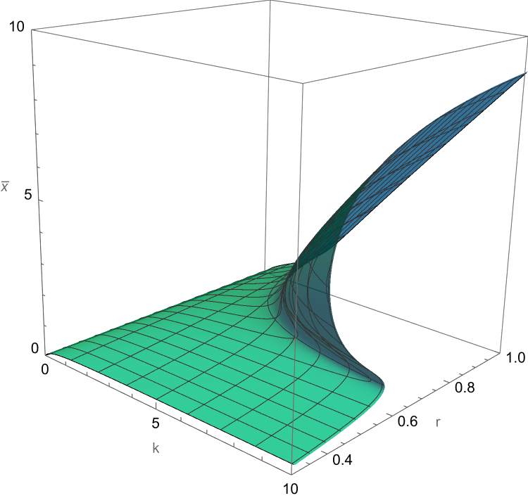
(a)

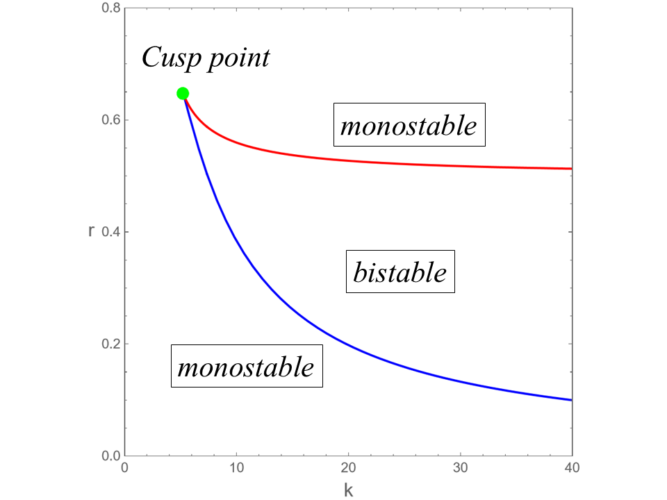
(b)

Figure 1: (a) The cusp catastrophe surface of eq.(14). (b) The bifurcation curve of eq.(15). The cusp point is $\bar{x}=\sqrt{3}$ and $(\bar{r},\bar{k})=\left(\displaystyle\frac{3\sqrt{3}}{8},3\sqrt{3}\right)$.

Based on eq.(2), the tropical discretization of eq.(13) brings about

$$x_{n+1}=\displaystyle\frac{x_{n}+\tau rx_{n}}{1+\tau\left(\displaystyle\frac{r}{k}x_{n}+\frac{x_{n}}{1+x_{n}^{2}}\right)},$$ (17)

where we set

$$f(x,r,k)=rx~~\text{and}~~g(x,r,k)=\displaystyle\frac{rx^{2}}{k}+\frac{x^{2}}{1+x^{2}}.$$ (18)

From the above proposition, eq.(17) also possesses the cusp bifurcation. It is confirmed that the fixed point of eq.(1) is identical to that of eq.(2)[11]. Then the fixed point of eq.(17), which is also $\bar{x}$, satisfies eq.(14). In addition, according to ref.[11], the stability of a fixed point $\bar{x}$ for eq.(2) depends on the sign of $\kappa(\bar{x})$, which is defined as

$$\kappa(\bar{x})=-\displaystyle\frac{2\bar{x}}{\bar{x}D(\bar{x})+2f(\bar{x})}.$$ (19)

We have confirmed that if $\bar{x}$ for eq.(1) is unstable, then $\bar{x}$ for eq.(2) is also unstable. And if $\bar{x}$ for eq.(1) is stable and $\kappa(\bar{x})<0$, then $\bar{x}$ for eq.(2) is also stable for any $\tau>0$. In the case of eq.(17), $\kappa(\bar{x})$ can be calculated as

$$\kappa(\bar{x}) = -\displaystyle\frac{2\bar{x}}{\bar{x}D(\bar{x})+2f(\bar{x},r,k)}$$ (20)

$$= -\frac{2}{D(\bar{x})+2r}=-\frac{2}{r+\displaystyle\frac{2\bar{x}^{3}}{(1+\bar{x}^{2})^{2}}}<0.$$

Therefore, the stability of $\bar{x}$ in eq.(13) is retained in eq.(17) for any $(r,k)$ and $\tau$. Furthermore, from the above proposition, eq.(17) exhibits the cusp bifurcation at the bifurcation point $(\bar{x},\bar{r},\bar{k})$ given in eq.(16). The bifurcation curves for eq.(17) are also given by eq.(15). Note that eq.(15) obtained from eq.(17) is independent of $\tau$. Here we note that eq.(17) becomes

$$x_{n+1}=\displaystyle\frac{r}{\displaystyle\frac{r}{k}+\frac{1}{1+x_{n}^{2}}}$$ (21)

in the limit of $\tau\to\infty$. Even in this limit for $\tau$, eq.(21) has the cusp bifurcation and the bifurcation curves are given by eq.(15).

4 Ultradiscretization

To derive the ultradiscrete max-plus equation for eq.(21), the variable transformations

$$x_{n}=e^{X_{n}/\varepsilon},~r=e^{R/\varepsilon},~k=e^{K/\varepsilon},$$ (22)

are applied. Then, the ultradiscrete limit

$$\lim_{\varepsilon\to+0}\varepsilon\log(e^{A/\varepsilon}+e^{B/\varepsilon})=\max(A,B)$$

provides the following max-plus equation,

$$X_{n+1}=R-\max(R-K,-\max(0,2X_{n})).$$ (23)

The dynamical properties of eq.(23) can be understood by the graph analysis (cobweb plot)[10]. First we consider the case $R>K$. Figure 2 shows the graphs of eq.(23) for (a) $K>0$ and (b) $K<0$. Since $\max(0,2X_{n})\geq 0$, eq.(23) becomes $X_{n+1}=K$ for any $X_{n}$. Therefore, $X_{n}=K$ is the unique fixed point and is stable.

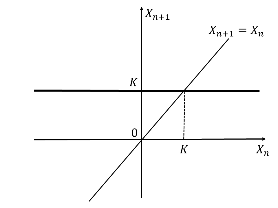
(a)

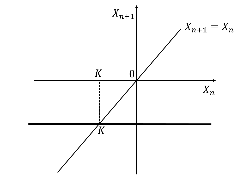
(b)

Figure 2: The graphs of eq.(23) for $R>K$. (a) $K>0$ and (b) $K<0$.

Next we consider the case $R<K$, where eq.(23) can be rewritten as

$$X_{n+1}=\begin{cases}R&\left(X_{n}<0\right),\\ 2X_{n}+R&\left(0\leq X_{n}<\displaystyle\frac{K-R}{2}\right),\\ K&\left(X_{n}\geq\displaystyle\frac{K-R}{2}\right).\end{cases}$$ (24)

Equation (24) is piecewise linear and can be divided into the five cases according to the type of intersection with the identity line $X_{n+1}=X_{n}$, as shown in Fig.3. Specifically, Fig.3 illustrates the following five cases: (a) $R>0$, (b) $R=0$, (c) $R<0$ and $K>-R$, (d) $R<0$ and $K=-R$, and (e) $R<0$ and $K<-R$. (a) For $R>0$, it is clear that $X_{n}=K$ is a stable fixed point. (b) For $R=0$, eq.(24) intersects the identity line at $X_{n}=K$ and $X_{n}=0$. It is found that $X_{n}=K$ is a stable fixed point and $X_{n}=0$ is a half-stable fixed point. (c) For $R<0$ and $K>-R$, eq.(24) has the three fixed points $X_{n}=K,\pm R$, where $X_{n}=+R,K$ are stable and $X_{n}=-R$ is unstable. (d) For $R<0$ and $K=-R$, eq.(24) intersects the identity line at $X_{n}=R$ and $X_{n}=K$. It is found that $X_{n}=R$ is a stable fixed point and $X_{n}=K$ is a half-stable fixed point. (e) For $R<0$ and $K<-R$, it is clear that $X_{n}=R$ is a stable fixed point. Therefore from above, the dynamical properties of eq.(23) are summarized as follows.

(1)

When $R>K$, $X_{n}=K$ is the unique fixed point and is stable.

(2)

When $R<K$,

(2-i)

if $R>0$, $X_{n}=K$ is the unique fixed point that is stable,

(2-ii)

if $R<0$ and $K>-R$, $X_{n}=\pm R$ $X_{n}=K$ are the fixed points. $+R$ and $K$ are stable (bistable) and $-R$ is unstable.

(2-iii)

if $R<0$ and $K<-R$, $X_{n}=R$ is the unique fixed point that is stable.

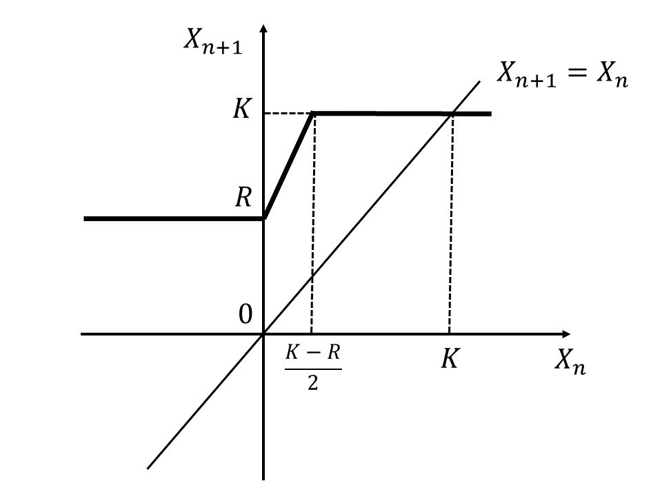
(a)

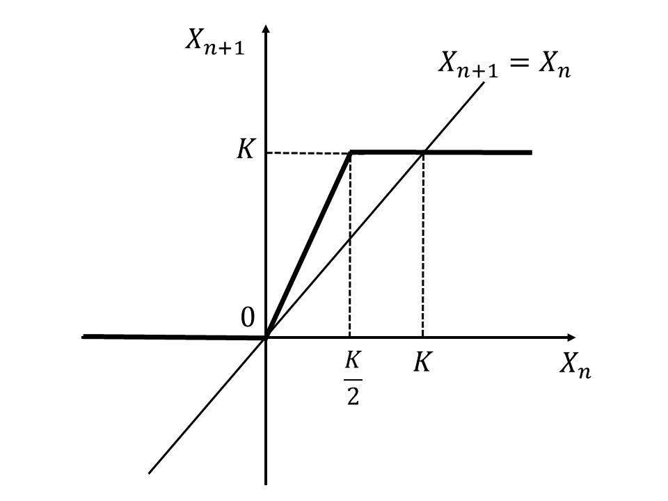
(b)

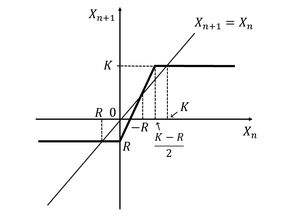
(c)

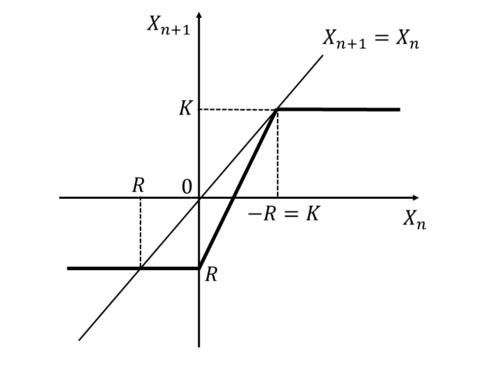
(d)

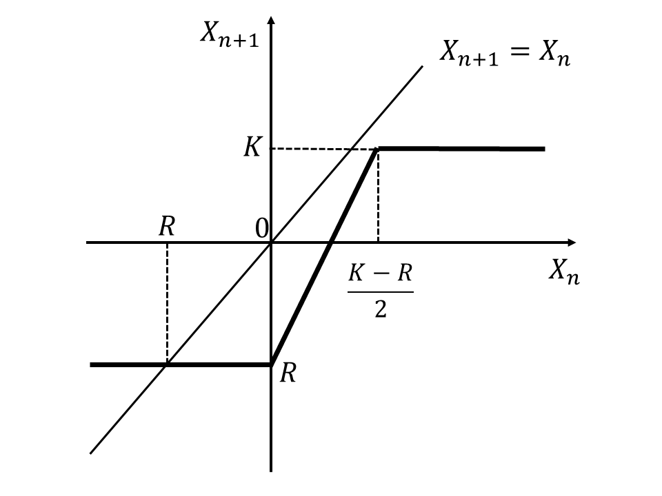
(e)

Figure 3: The graphs of eq.(23) for (a) $R>0$, (b) $R=0$, (c) $R<0$ and $K>-R$, (d) $R<0$ and $K=-R$, and (e) $R<0$ and $K<-R$.

Figure 4(a) shows the cusp catastrophe surface for eq.(23), which is plotted according to the above summary. And the cusp bifurcation curve for eq.(23) is also shown in Fig.4(b). The cusp point is $X=0$ at $(R,K)=(0,0)$. A comparison between Figs. 1 and 4 indicates that the features of the cusp bifurcation are retained even after piecewise linearization through ultradiscretization.

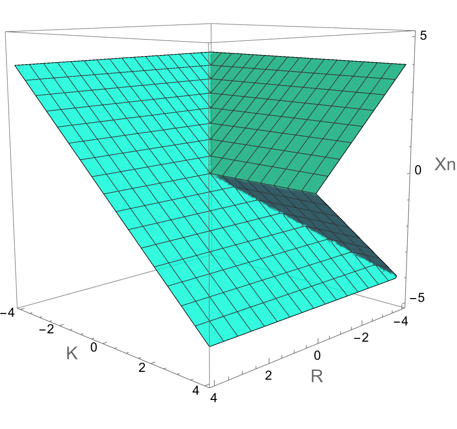
(a)

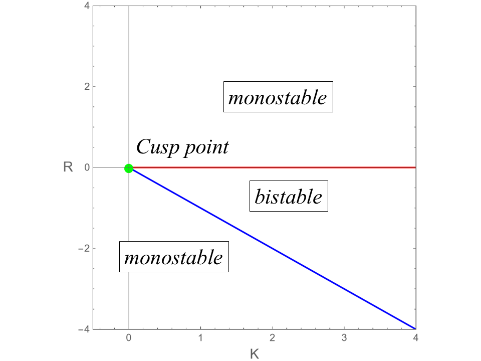
(b)

Figure 4: (a) The cusp catastrophe surface for eq.(23). (b) The bifurcation curve for eq.(23). The cusp point is $X_{n}=0$ at $(R,K)=(0,0)$.

5 Discussion

We demonstrate another example. The following equation is the biochemical model having the cusp bifurcation, proposed by J. Lewis[1, 22].

$$\frac{dx}{dt}=G(x,p,q)=p-qx+\frac{x^{2}}{1+x^{2}},$$ (25)

where $x\geq 0$ and $p,q>0$. Equation (25) possesses the fixed points, $\bar{x}$, which satisfy $G(\bar{x},p,q)=0$:

$$q\bar{x}-p=\frac{\bar{x}^{2}}{1+\bar{x}^{2}}.$$ (26)

Figure 5(a) shows the cusp catastrophe surface given by eq.(26). The cusp bifurcation curve are also derived from $G(\bar{x},p,q)=0$ and $\displaystyle\frac{\partial}{\partial x}G(\bar{x},p,q)=0$, which yield

$$p=\frac{(1-\bar{x}^{2})\bar{x}^{2}}{(1+\bar{x}^{2})^{2}},\;\;\;\;\;q=\frac{2\bar{x}}{\left(1+\bar{x}^{2}\right)^{2}}.$$ (27)

The bifurcation curve given by eq. (27) is shown in Fig. 5 (b) as functions of $p$ and $q$. And the cusp point of eq.(25) is $\displaystyle\bar{x}=\frac{1}{\sqrt{3}}$ at $\displaystyle\left(\bar{p},\bar{q}\right)=\left(\frac{1}{8},\frac{3\sqrt{3}}{8}\right)$. Note that eq.(25) satisfies the cusp bifurcation conditions: $\displaystyle G(\bar{x},\bar{p},\bar{q})=\frac{\partial G(\bar{x},\bar{p},\bar{q})}{\partial x}=\frac{\partial^{2}G(\bar{x},\bar{p},\bar{q})}{\partial x^{2}}=0$, $\displaystyle\frac{\partial^{3}G(\bar{x},\bar{p},\bar{q})}{\partial x^{3}}=-\frac{27\sqrt{3}}{16}\neq 0$, and $\displaystyle\frac{\partial G(\bar{x},\bar{p},\bar{q})}{\partial p}\frac{\partial^{2}G(\bar{x},\bar{p},\bar{q})}{\partial x\partial q}-\frac{\partial G(\bar{x},\bar{p},\bar{q})}{\partial q}\frac{\partial^{2}G(\bar{x},\bar{p},\bar{q})}{\partial x\partial p}=-1\neq 0$.

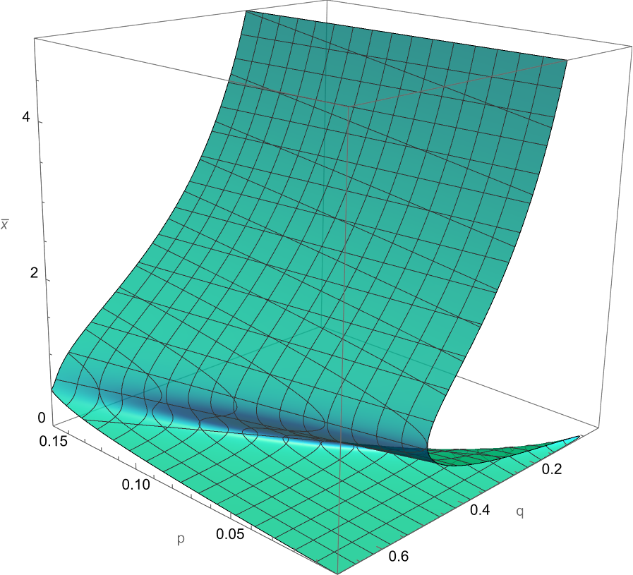
(a)

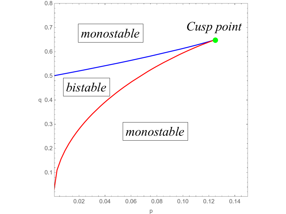
(b)

Figure 5: (a) The cusp catastrophe surface of eq.(26). (b) The bifurcation curve of eq.(27). The cusp point is $\displaystyle\bar{x}=\frac{1}{\sqrt{3}}$ at $\displaystyle(\bar{p},\bar{q})=\left(\frac{1}{8},\frac{3\sqrt{3}}{8}\right)$.

The discretized equation of eq.(25) can be obtained as follows by tropical discretization based on eq.(2) by setting $f(x,p,q)=p+\displaystyle\frac{x^{2}}{1+x^{2}}$ and $g(x,p,q)=qx$,

$$x_{n+1}=\displaystyle\frac{x_{n}+\tau\left(p+\displaystyle\frac{x^{2}_{n}}{1+x_{n}^{2}}\right)}{1+\tau q}.$$ (28)

From the above proposition, it is found that eq.(28) also exhibits the cusp bifurcation. When $\tau\to\infty$, eq.(28) becomes

$$x_{n+1}=\displaystyle\frac{p}{q}+\frac{x^{2}_{n}}{q(1+x_{n}^{2})}.$$ (29)

Note that the fixed points and the bifurcation curve for eq.(29) coincide with those of eq.(25).

Applying the variable transformations,

$$x_{n}=e^{X_{n}/\varepsilon},~p=e^{P/\varepsilon},~q=e^{Q/\varepsilon},$$ (30)

to eq.(29), and taking the ultradiscrete limit, the following max-plus equation can be obtained,

$$X_{n+1} = \max(P-Q,2X_{n}-Q-\max(0,2X_{n}))$$ (31)

$$= -Q+\max(P,-\max(0,-2X_{n})).$$

Considering the transformation $X_{n}\to-X_{n}$, eq.(31) becomes

$$X_{n+1}=Q-\max(P,-\max(0,2X_{n})).$$ (32)

Comparing eq.(32) with eq.(23), it is found that these equations are identical when we set

$$Q=R,\;\;\;P=R-K.$$ (33)

Therefore, Lewis model, eq.(25), brings about the same piecewise linear cusp bifurcation as Ludwig model, eq.(13). Note that the original continuous Lewis model has different terms from the original continuous Ludwig model. However, the ultradiscrete equations for the Ludwig model and the Lewis model are essentially identical, and the common dynamical structure can be extracted and expressed with the same max-plus representation.

6 Conclusion

In this paper, we have reported the investigation of the cusp bifurcation in the one-dimensional discrete dynamical systems derived via tropical discretization and in the max-plus dynamical systems obtained by ultradiscretization. Based on our proposed proposition, we show that these dynamical systems retain the cusp bifurcation of the original continuous differential equation, using the Ludwig model and Lewis model as representative examples. The cusp bifurcation point, curve, and surface of the tropically discretized systems coincide with those of the original differential systems. Furthermore, the ultradiscrete max-plus equations can also express the cusp bifurcation properties in a piecewise linear form. We expect that the tropical and ultradiscrete approaches provide a promising framework for describing nonlinear and nonequilibrium phenomena with discrete and max-plus dynamical systems.

Acknowledgement

The authors are grateful to Prof. M. Murata, Prof. K. Matsuya, Prof. D. Takahashi, Prof. R. Willox, Prof. H. Ujino, Prof. Y. Sato, Prof. A. Shudo, Prof. Emeritus Y. Aizawa, Prof. T. Yamamoto, and Prof. Emeritus A. Kitada for useful comments and encouragements. This work was supported by JSPS KAKENHI Grant Numbers 22K03442, 22K13963, 25K00212, and 25K07140.

References

- [1] S. H. Strogatz, Nonlinear Dynamics and Chaos (Westview Press, U.S. 1994).
- [2] N. Boccara, Modeling Complex Systems (Springer, New York, 2004).
- [3] S. Wolfram, Phys. Scr. 1985, 170 (1985).
- [4] T. Tokihiro, Discrete Integrable Systems (edited by B. Grammaticos, T. Tamizhmani, and Y. Kosmann-Schwarzbach, Springer, Berlin, Heidelberg, 2004), pp. 383–424.
- [5] M. Murata, J. Difference. Equ. Appl., 19, 1008 (2013).
- [6] K. Matsuya and M. Murata, Discrete Contin. Dyn. Syst. B 20, 173 (2015).
- [7] S. Ohmori and Y. Yamazaki, J. Phys. Soc. Jpn. 85, 045001 (2016).
- [8] A. S. Carstea, J. Satsuma, R. Willox and B. Grammaticos, Continuous, discrete and ultra- discrete models of an inflammatory response, Physica A 364, 276 (2006).
- [9] R. Willox, A. Ramani, J. Satsuma, and B. Grammaticos, Physica A 385, 473 (2007).
- [10] S. Ohmori and Y. Yamazaki, J. Math. Phys. 61 122702 (2020).
- [11] S. Ohmori and Y. Yamazaki, J. Math. Phys. 64, 042704 (2023).
- [12] Y. Yamazaki and S. Ohmori, J. Phys. Soc. Jpn. 90 103001 (2021).
- [13] S. Ohmori and Y. Yamazaki, unpublished (arXiv:2103.16777v1).
- [14] S. Ohmori and Y. Yamazaki, JSIAM Letters 14 127 (2022).
- [15] S. Ohmori and Y. Yamazaki, JSIAM Letters, 15 73 (2023).
- [16] Y. Yamazaki and S. Ohmori, Prog. Theor. Exp. Phys. 2023 081A01 (2023).
- [17] S. Ohmori and Y. Yamazaki, in press (arXiv:2305.05908).
- [18] S. Ohmori and Y. Yamazaki, J. Math. Phys. 65 082705 (2024).
- [19] Y. Yamazaki and S. Ohmori, JSIAM Letters 16 85 (2024).
- [20] Y. A. Kuznetsov, Elements of Applied Bifurcation Theory (4th ed., Springer, 2023).
- [21] D. Ludwig, D. D. Jones, C. S. Holling, J. Anim. Ecol., 47, 315 (1978).
- [22] J. Lewis, J. M. W. Slack, and L. Wolpert, J. Theor. Biol. 65 579 (1977).