Sensing for Free: Learn to Localize More Sources than Antennas without Pilots

Abstract

Integrated sensing and communication (ISAC) represents a key paradigm for future wireless networks. However, existing approaches often require waveform modifications, dedicated pilots, or additional overhead that complicates standards integration. We propose “sensing for free”—performing multi-source localization without pilots by reusing standard uplink data symbols, where sensing happens simultaneously with data transmission, making it directly compatible with the 3GPP 5G NR and 6G specifications. With the ever-increasing number of devices in dense 6G networks, this approach becomes particularly compelling when combined with sparse arrays, which can localize a much larger number of sources compared to uniform arrays through the enlarged virtual array. However, existing pilot-free multi-source localization algorithms for sparse arrays have numerous drawbacks. They mostly first reconstruct an extended covariance matrix and then apply subspace methods, which incur prohibitive cubic complexity while being limited to second-order statistics. Performance degrades under non-Gaussian modulated data symbols and small snapshot counts. Also, the higher-order statistics that could further enhance the localization capability remain unexploited. We address these challenges with an attention-only transformer that directly processes raw signal snapshots for grid-less end-to-end direction-of-arrival (DOA) estimation. The model efficiently captures higher-order statistics while being permutation-invariant and adaptive to varying snapshot counts. Our algorithm greatly outperforms state-of-the-art artificial intelligence (AI)-based benchmarks with over $30\times$ reduction in parameters and runtime, and enjoys excellent generalization under practical mismatches. Applied to multi-user MIMO beam training, our algorithm can localize the uplink DOAs of multiple users simultaneously in the data transmission stage. Through angular reciprocity, estimated uplink DOAs significantly prune downlink beam sweeping candidates and enhance system throughput via sensing-assisted beam management. This work demonstrates how reusing existing data transmission for sensing can enhance both multi-source localization and beam management, two key AI-for-communication use cases in 3GPP efforts towards 6G.

I Introduction

I-A Background

Integrated sensing and communication (ISAC) has emerged as a key paradigm for 6G wireless networks, attracting significant interest across academia, industry, and also standardization bodies [1, 2, 3, 4, 5, 6]. For instance, ISAC is recognized as one of the six major use cases of 6G [2], and has been actively studied by the 3rd generation partnership project (3GPP), e.g., TR 22.837 in Release 19 and the ongoing discussions for Release 20 [4, 5, 6]. The basic idea is to enable the communication infrastructure itself to perform sensing functions, typically by repurposing the communication signals for radar-like tasks. Existing ISAC approaches, however, often require modifications to the waveforms or frame structures to embed sensing capabilities, which can undermine the communication performance or demand upgrades to the existing infrastructure. By contrast, we are interested in a scenario where sensing can be achieved “for free” during regular data transmissions, without using additional pilots or radio resources. In particular, we focus on the uplink of a cellular system, where a multi-antenna base station (BS) attempts to localize multiple sources by processing the unknown uplink data symbols. This type of ISAC would allow next-generation networks to gain situational awareness with no extra overhead, making it easy for practical deployment.

At the same time, the demand to localize a large number of sources has become increasingly prominent, driven by the proliferation of massive internet of things (IoT) [7], unmanned aerial vehicles (UAV) communications [8], and low-altitude economy [9]. Using a conventional $M$-element uniform linear array (ULA), subspace methods such as multiple signal classification (MUSIC) can only resolve at most $M-1$ uncorrelated sources since the noise subspace must be non-trivial [10]. To overcome such a limitation, sparse linear arrays (SLAs) have been proposed, such as nested [11], co-prime [12], and minimum redundancy arrays (MRAs) [13], which sparsely deploy antennas over a large aperture to enhance the sensing capability. A properly designed $M$-antenna SLA can form a much larger virtual array, enabling the localization of $O(M^{2})$ uncorrelated sources using extended covariance matrix, far more than the number of antennas $M$ [14]. These advantages have motivated interest in considering SLAs for ISAC systems [15]. In [16], the authors found that by exploiting the virtual array for localization and physical array for communications, SLAs can achieve both enhanced sensing capability and competitive communication performance. Some recent investigations also focused on the advantages of SLAs in enhancing communication performance [17, 18, 19]. In fact, SLAs represent both established and emerging paradigms in wireless communications. In MIMO systems with antenna selection [20] or switch-based hybrid analog-digital beamforming [21], activating a subset of antennas effectively creates an SLA. Moreover, recently emerging flexible-antenna technologies, such as fluid [22] and movable [23] antenna systems, deploy antennas in flexible positions within a large aperture, and can also be naturally configured as SLAs to exploit their advantages in sensing and localization. The algorithms studied in this work are hence broadly applicable. We show the variants of SLAs in Fig. 1.

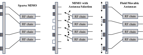
Figure 1: SLAs and their variants, including but not limited to MIMO systems with antenna selection [20] and fluid/movable antennas [22, 23].

In this paper, we consider ISAC with SLAs and ask the following question: Can a base station localize more sources than its number of antennas during regular data transmission, without pilots or extra resources? We investigate DL-based algorithms that provide affirmative answers to this question that are accurate, fast, and robust. We further showcase the fundamental value of such “sensing for free” capability for wireless system design, in particular beam management.

I-B Related Works

I-B1 Multi-Source Localization with SLAs

While pilot-free ISAC with sparse arrays is an emerging idea in wireless communications [15], a closely related problem, i.e., sparse array DOA estimation, has been extensively studied in array signal processing. Classical subspace-based multi-source localization algorithms, including MUSIC [10] and Root-MUSIC [24], rely on eigen-decomposition of the sample spatial covariance matrix (SCM) to separate signal and noise subspaces. For SLAs, the key challenge is reconstructing the missing entries of the SCM to exploit the larger virtual aperture, which can be formulated as a constrained optimization problem using the maximum likelihood principle. Optimization techniques, such as semi-definite programming (SDP) [25], nuclear norm [26] and atomic norm [27] minimization, Wasserstein distance minimization [28], etc., have been proposed. Recently, DL methods have also been studied to reconstruct the extended SCM for subsequent subspace methods. Most of them use convolutional neural networks (CNNs) as the backbone. In [29], leveraging the semidefinite property of the SCM, the authors proposed using CNNs to output auxiliary matrices whose Gramians approximate the extended SCM. In [30], the authors proposed estimating the first row to construct Toeplitz-structured SCMs, exploiting the inherent structure of array response matrices. In [31], a subspace representation learning approach was proposed that prioritizes signal subspace preservation over exact SCM reconstruction. These DL-based methods employ various loss functions including Frobenius norm [29, 30], affine invariant distance [29] and subspace distance [31], such as principal angles between subspaces [32].

While these constitute important related works, they represent signal processing approaches that differ fundamentally from the problem addressed in this study. First, these methods are predicated on Gaussian signal assumptions and rely exclusively on second-order statistics, specifically the SCM. Although the SCM provides sufficient statistics for Gaussian processes, modulated data symbols in practical communication systems exhibit non-Gaussian characteristics, leading to suboptimal performance when applying these approaches. Second, computational complexity presents a significant limitation. These methods employ a two-stage pipeline comprising SCM reconstruction followed by classical subspace methods, necessitating eigen-decomposition of the SCM and exhaustive spectrum search to separate signal and noise subspaces. This results in prohibitive computational complexity scaling as $O(N^{3})$, where $N\gg M$ represents the number of elements the virtual array corresponding to the SLA. Alternative approaches that attempt to exploit higher-order statistics, such as MUSIC-like algorithms leveraging fourth-order cumulants, incur an even more prohibitive complexity of $O(N^{6})$ [33, 34]. Third, prior works typically assume the availability of hundreds of signal snapshots for DOA estimation, which is unrealistic given the short coherence times in communication systems. Under practical constraints of limited snapshots, the sample SCM becomes unreliable and as a result leads to performance degradation of subspace methods.

I-B2 Sensing-Assisted Beam Management

Angular reciprocity in massive MIMO systems enables sensing-assisted beam management by leveraging the shared angular sparsity between uplink and downlink channels, which is observed even in frequency division duplex (FDD) systems [35, 36]. In [37], the authors demonstrated directional training frameworks leveraging this reciprocity through measurement results. While they did not study specific algorithms for uplink DOA estimation, the results laid the foundation of sensing-assisted beam training. Recent advances in multimodal ISAC have further explored richer sensing paradigms, integrating vision, radio, and radar data for reducing the overhead and improving the accuracy of beam prediction [38, 39, 40].

While these works have established the fundamentals and benefits of sensing-assisted beam management, they either rely on dedicated pilots for angular parameter estimation or require additional sensing modalities and corresponding infrastructure upgrades. This leaves an opportunity for “sensing for free” approaches that can achieve sensing-assisted beam management without requiring additional resources or system modifications.

I-C Contributions

The contributions of this paper are mainly two-fold, which are summarized from system and algorithmic perspectives.

From a system standpoint, we demonstrate that, by leveraging unknown uplink data symbols already present in each frame, multi-source localization can be achieved at the same time with data transmission, without any dedicated overhead. Because the method leaves frame structures and waveforms untouched, it could be easily embedded into forthcoming wireless systems. Exploiting the enlarged virtual aperture of SLAs, the BS can accurately localize the DOAs for more users than physical antennas. These DOA estimates, in turn, are accurate enough to enable a significant pruning of the downlink beam sweeping candidates, remarkably reducing beam management overhead and enhancing system throughput. The results in our study motivate a rethinking of how uplink data symbols can be better harnessed to facilitate the ISAC functionality.

From an algorithmic perspective, conventional multi-source localization algorithms for SLAs rely on covariance reconstruction followed by subspace methods. They are both computationally expensive and prone to performance loss under the non-Gaussian data symbols and the limited snapshots. We circumvent subspace methods with an attention-only transformer that processes raw signal snapshots of SLAs to efficiently capture higher-order statistics for grid-less end-to-end DOA estimation, avoiding both covariance reconstruction and decomposition. Our algorithm consistently outperforms state-of-the-art benchmarks across a wide signal-to-noise-ratio (SNR) range while offering a significant reduction of over $30\times$ in computational complexity under typical system settings. It also generalizes under various practical mismatches, and scales gracefully to large-scale arrays. Extensive simulation results and ablation studies confirm these advantages, establishing a novel paradigm for pilot-free multi-source localization and ISAC with sparse arrays.

I-D Paper Organization and Notation

The remaining parts of this article are organized as follows. In Section II, we discuss the preliminaries of the system model and define the problem. In Section III, we introduce the prior arts of multi-source localization with sparse arrays and their limitations. In Section IV, we propose the Snap-TF algorithm and discuss its properties and insights. In Section V, extensive simulation results are presented to demonstrate the advantages of the proposed algorithm from various aspects. In Section VI, we discuss the further application of the proposed algorithm to sensing-assisted beam management of multi-user MIMO (MU-MIMO) systems. Lastly, we conclude the paper in Section VII.

Notation: Throughout this work, we denote scalars by italic lowercase letters, column vectors with boldface lowercase letters, while matrices by boldface uppercase letters, respectively. For any vector $\mathbf{a}$, $[\mathbf{a}]_{1:i}$ denotes its first $i$ elements. For any matrix $\mathbf{A}$, $\mathbf{A}^{*}$, $\mathbf{A}^{T}$, $\mathbf{A}^{H}$, $[\mathbf{A}]_{:,1:i}$, and $[\mathbf{A}]_{i,j}$ are its conjugate, transpose, conjugate transpose, the first $i$ columns, and the $(i,j)$-th element, respectively. The Euclidean and Frobenius norms are written as $\lVert\mathbf{a}\rVert_{2}$ and $\lVert\mathbf{A}\rVert_{F}$, respectively, and $|\cdot|$ is the cardinality of a set. The operators $\operatorname{diag}(\cdot)$, $\Re({\cdot})$, and $\Im({\cdot})$ generate a diagonal matrix and extract the real and imaginary parts, respectively. The imaginary unit is $j$. The natural logarithm is denoted by $\ln(\cdot)$.

II Preliminaries

II-A System Model with Sparse MIMO Arrays

Assuming that there are $K$ narrowband and far-field sources $\{s_{k}\}_{k=1}^{K}$ with a carrier wavelength $\lambda$ impinging upon a BS with a linear array from DOAs $\bm{\theta}=\{\theta_{1},\theta_{2},\ldots,\theta_{k}\}$. We assume the DOAs are independent and identically distributed (i.i.d.) and are drawn randomly from a uniform distribution $\mathcal{U}(\theta_{\min},\theta_{\max})$, where $0\leq\theta_{\min}\leq\theta_{\max}\leq\pi$ are the minimum and maximum values of the angle range, respectively. The minimum angle separation of DOAs is defined as $\Delta_{\bm{\theta},\text{min}}\triangleq\min_{i\neq j}|\theta_{i}-\theta_{j}|$. The array is equipped with $M$ antennas with an array aperture of $(N-1)d$ where $N\geq M$. It can be either uniform or sparse, where the antenna positions are chosen from the integer multiples of half the wavelength $d=\frac{\lambda}{2}$. We use $\bm{\Omega}=\{\Omega_{1},\Omega_{2},\ldots,\Omega_{M}\}$ to denote the indices of antennas, where $\Omega_{m}$ is an integer representing that the position of the $m$-th antenna is $\Omega_{m}d$. In general, we configure that $1=\Omega_{1}<\Omega_{2}<\ldots<\Omega_{M}=N$. For the special case of ULAs, we have $M=N$ and $\bm{\Omega}=\{1,2,\ldots,N\}$. Fig. 2 shows a comparison of uniform and sparse arrays.

The signals are transmitted from the sources to the array for $T$ snapshots. For each snapshot $t\in\{1,2,\ldots,T\}$, the received signal at the array, i.e., $\mathbf{y}_{\bm{\Omega}}(t)\in\mathbb{C}^{M\times 1}$, is given by

$$\mathbf{y}_{\bm{\Omega}}(t) =\sum_{k=1}^{K}p_{k}\mathbf{a}_{\bm{\Omega}}(\theta_{k})s_{k}(t)+\mathbf{n}_{\bm{\Omega}}(t)$$ (1)

$$=\mathbf{A}_{\bm{\Omega}}(\bm{\theta})\mathbf{P}\mathbf{\mathbf{s}}(t)+\mathbf{n}_{\bm{\Omega}}(t)$$

$$=\mathbf{H}_{\bm{\Omega}}\mathbf{\mathbf{s}}(t)+\mathbf{n}_{\bm{\Omega}}(t),$$

where $p_{k}\in\mathbb{C}$, $s_{k}(t)\in\mathbb{C}$, and $\mathbf{a}_{\bm{\Omega}}(\theta_{k})\in\mathbb{C}^{M\times 1}$ are the path loss, the source signal, and the array response vector of the $k$-th source, respectively. In addition, $\mathbf{A}_{\bm{\Omega}}(\bm{\theta})=[\mathbf{a}_{\bm{\Omega}}(\theta_{1}),\mathbf{a}_{\bm{\Omega}}(\theta_{2}),\ldots,\mathbf{a}_{\bm{\Omega}}(\theta_{K})]\text{$\in\mathbb{C}^{M\times K}$}$ is the array response matrix, $\mathbf{P}=\operatorname{diag}(p_{1},p_{2},\ldots,p_{K})\in\mathbb{C}^{K\times K}$ is the matrix form of the path loss, and $\mathbf{s}(t)=[s_{1}(t),s_{2}(t),\ldots,s_{K}(t)]^{T}\in\mathbb{C}^{K\times 1}$ is the collection of source signals. The multi-user MIMO channel of the SLA is denoted by $\mathbf{H}_{\bm{\Omega}}=\mathbf{A}_{\bm{\Omega}}(\bm{\theta})\mathbf{P}\in\mathbb{C}^{M\times K}$. The noise is given by $\mathbf{n}_{\bm{\Omega}}(t)\in\mathbb{C}^{M\times 1}$. The source signals $\mathbf{s}(t)$ and the noise $\mathbf{n}_{\bm{\Omega}}(t)$ are independent of each other, and they are both temporally uncorrelated across different snapshots. The array response vector $\mathbf{\mathbf{a}}_{\bm{\Omega}}(\theta_{k})$ is

$$\mathbf{\mathbf{a}}_{\bm{\Omega}}(\theta_{k})=\left[e^{j\pi(\Omega_{1}-1)\sin(\theta_{k})},\ldots,e^{j\pi(\Omega_{M}-1)\sin(\theta_{k})}\right]^{T}.$$ (2)

The elements of the SLA array response vector $\mathbf{\mathbf{a}}_{\bm{\Omega}}(\theta_{k})$ are selected from those of the ULA array response vector $\mathbf{\mathbf{a}}(\theta_{k})$ with $\mathbf{\mathbf{a}}_{\bm{\Omega}}(\theta_{k})=\bm{\Gamma}_{\bm{\Omega}}\mathbf{\mathbf{a}}(\theta_{k})$, where $\mathbf{\mathbf{a}}(\theta_{k})=[1,e^{j\pi\sin(\theta_{k})},\ldots,e^{j\pi(N-1)\sin(\theta_{k})}]$ and $\bm{\Gamma}_{\bm{\Omega}}\in\mathbb{R}^{M\times N}$ is a row selection matrix whose elements are ones at the $\Omega_{m}$-th position of the $m$-th column and zeros elsewhere. Similarly, we have $\mathbf{A}_{\bm{\Omega}}(\bm{\theta})=\bm{\Gamma}_{\bm{\Omega}}\mathbf{A}(\bm{\theta})$, with $\mathbf{A}(\bm{\theta})=[\mathbf{a}(\theta_{1}),\mathbf{a}(\theta_{2}),\ldots,\mathbf{a}(\theta_{K})]\text{$\in\mathbb{C}^{N\times K}$}$ being the ULA array response matrix, and $\mathbf{y}_{\bm{\Omega}}(t)=\bm{\Gamma}_{\bm{\Omega}}\mathbf{y}(t)$, where $\mathbf{y}(t)\in\mathbb{C}^{N\times 1}$ denotes the received signals by the ULA. We make the following assumptions on the source signals and the noise:

• Source signals ${s_{k}(t)}$ are all zero-mean random processes. We consider both Gaussian and non-Gaussian signals, and assume that each $s_{k}(t)$ is independent identically distributed (i.i.d.) across snapshots. The signal $s_{k}(t)$ can either be circular complex Gaussian or practical non-Gaussian modulated symbols, such as QPSK (quadrature phase shift keying) and 16QAM (quadrature modulation), etc. We assume that the source signals are mutually independent and also uncorrelated with the noise. We consider the case where the source signals $s_{k}(t)$ are unknown during the estimation process, corresponding to unknown uplink data symbols. Hence, our multi-source DOA estimation happens simultaneously with uplink data transmission, and requires no additional overhead and no modifications to the frame structures or waveforms.

• Noise $\mathbf{n}_{\bm{\Omega}}(t)$ is assumed zero-mean Gaussian distributed and independent across snapshots, following $\mathcal{CN}(\mathbf{0},\eta\mathbf{I})$, where $\eta$ is the noise power.

  

  (a)

  

  (b)

  Figure 2: An comparison of 5-element uniform and sparse MIMO arrays. The top array is a ULA with $M=N=5$, and the bottom one is a special SLA, called minimum redundancy array (MRA) [13], with $M=5$ and $N=10$. The black circles denote the positions where the antennas are placed.

After $T$ snapshots, we stack the received signal snapshots into the matrix form. For the full $N$-element ULA, we have $\mathbf{Y}=[\mathbf{y}_{\bm{}}(1),\mathbf{y}_{\bm{}}(2),\ldots,\mathbf{y}_{\bm{}}(T)]\in\mathbb{C}^{N\times T}$, while for the $M$-element SLA, we obtain $\mathbf{Y}_{\bm{\Omega}}=[\mathbf{y}_{\bm{\Omega}}(1),\mathbf{y}_{\bm{\Omega}}(2),\ldots,\mathbf{y}_{\bm{\Omega}}(T)]\in\mathbb{C}^{M\times T},$ where $\mathbf{Y}_{\bm{\Omega}}=\bm{\Gamma}_{\bm{\Omega}}\mathbf{Y}$ through the row selection matrix $\bm{\Gamma}_{\bm{\Omega}}\in\mathbb{R}^{M\times N}$. We next define the noiseless spatial covariance matrices (SCMs). The full $N$-element ULA has noiseless SCM $\mathbf{R}=\mathbf{A}(\bm{\theta})\mathbf{P}\mathbf{A}^{H}(\bm{\theta})\in\mathbb{C}^{N\times N}$. The corresponding noiseless SCM for the $M$-element SLA is $\mathbf{R}_{\bm{\Omega}}=\bm{\Gamma}_{\bm{\Omega}}\mathbf{R}\bm{\Gamma}_{\bm{\Omega}}^{T}\in\mathbb{C}^{M\times M}$, obtained by applying the same row selection matrix $\bm{\Gamma}_{\bm{\Omega}}$. In practice, the sample SCMs of SLA and ULA are obtained based on the noisy received signal snapshots, which are respectively given by $\tilde{\mathbf{R}}_{\bm{\Omega}}\triangleq\frac{1}{T}\mathbf{Y}_{\bm{\Omega}}\mathbf{Y}_{\bm{\Omega}}^{H}$ and $\tilde{\mathbf{R}}\triangleq\frac{1}{T}\mathbf{Y}\mathbf{Y}^{H}$.

II-B Problem Statement

Based on $T$ snapshots of received signals at the $M$-element SLA, i.e., $\mathbf{Y}_{\bm{\Omega}}$, the target is to estimate the DOAs of $K$ sources, i.e., $\bm{\theta}$, in which $K$ could be larger than $M$. We note that the sources $\mathbf{s}(t)$ are unknown uplink data symbols, in contrast to pilot symbols that are perfectly known [41]. The multi-source localization is carried out at the same time during data transmission and thus requires no additional time or frequency resources. As the true and estimated DOAs are two sets, to remove the permutation ambiguity when comparing their distance, we define the mean square error (MSE) of the estimated angles $\hat{\bm{\theta}}$ and the ground-truth $\bm{\theta}$ as

$$\operatorname{MSE}(\hat{\boldsymbol{\theta}},\boldsymbol{\theta})=\frac{1}{K}\min_{\boldsymbol{\Pi}_{K}\in\mathcal{P}_{K}}\left\|\boldsymbol{\Pi}_{K}\hat{\boldsymbol{\theta}}-\boldsymbol{\theta}\right\|_{2}^{2},$$ (3)

where $\boldsymbol{\Pi}_{K}$ represents a specific $K\times K$ permutation matrix while $\mathcal{P}_{K}$ denotes the set of all possible $K\times K$ permutation matrices. The minimum can be easily obtained by sorting both $\hat{\boldsymbol{\theta}}$ and ${\boldsymbol{\theta}}$ according to the rearrangement inequality [42], which is widely used to evaluate the DOA estimation performance.

The value of the problem is that, once this is achieved, we can localize more sources than the number of physical antennas by using unknown data symbols, at the same time of data transmission, without using any additional pilots or radio resources. In this sense, sensing is achieved “for free”.

III Prior Art

While there are no previous works for ISAC with sparse arrays using unknown data symbols, we summarize the state-of-the-art DL-based algorithms for sparse array DOA estimation using Gaussian signals, which will serve as important benchmarks later. The dataset is defined as $\{\mathbf{Y}_{\bm{\Omega}}^{(i)},K^{(i)},\bm{\theta}^{(i)}\}_{i=1}^{I}$, where $I$ is the number of samples in the dataset and the superscript $(\cdot)^{(i)}$ denotes the $i$-th sample. For the $i$-th data sample, the DOA estimation algorithm takes both the received signal snapshots at the SLA, i.e., $\mathbf{Y}_{\bm{\Omega}}^{(i)}\in\mathbb{C}^{M\times T}$, and the number of sources, i.e., $K^{(i)}$ as inputs, while the outputs are the estimated DOAs whose ground-truth labels are $\bm{\theta}^{(i)}\in\mathbb{R}^{K\times 1}$.

Most previous methods follow a two-stage pipeline. First, they learn to reconstruct the noiseless SCM of the corresponding virtual ULA, i.e., ${\mathbf{R}}^{(i)}$, from the sample SCM of the ULA, i.e., $\tilde{\mathbf{R}}_{\bm{\Omega}}^{(i)}$, both of which can be obtained based on the dataset as described earlier. Second, they apply subspace methods, e.g., MUSIC or Root-MUSIC, for DOA estimation [29, 30, 31]. These approaches employ convolutional neural networks (CNNs) as backbones, denoted by $f_{\mathcal{W}}(\cdot)$ with $\mathcal{W}$ being the network parameters, and assume that the transmitted signals $\mathbf{s}(t)$ are Gaussian distributed. The main differences of existing DL-based subspace methods lies in the model output and loss function, as listed in Table I.

In the following, we begin by summarizing the two key steps of the existing algorithms, i.e., covariance reconstruction and subspace methods, before discussing their limitations for multi-source localization with unknown uplink symbols.

TABLE I: Existing learning methods for sparse array DOA estimation

Method	Model output	Loss function
DCR-G-Fro [29]	$\hat{\mathbf{R}}=f_{\mathcal{W}}(\tilde{\mathbf{R}}_{\bm{\Omega}})f_{\mathcal{W}}^{H}(\tilde{\mathbf{R}}_{\bm{\Omega}})$	$\|\hat{\mathbf{R}}-\mathbf{R}\|_{F}$
DCR-G-Aff [29]	$\hat{\mathbf{R}}=f_{\mathcal{W}}(\tilde{\mathbf{R}}_{\bm{\Omega}})f_{\mathcal{W}}^{H}(\tilde{\mathbf{R}}_{\bm{\Omega}})$	$\bigl{\|}\ln\bigl{(}\mathbf{R}^{-\tfrac{1}{2}}\,\hat{\mathbf{R}}\,\mathbf{R}^{-\tfrac{1}{2}}\bigr{)}\bigr{\|}_{F}$
DCR-T [30]	$\hat{\mathbf{v}}=f_{\mathcal{W}}(\tilde{\mathbf{R}}_{\bm{\Omega}}),\hat{\mathbf{R}}=\operatorname{Toep}(\hat{\mathbf{v}})$	$\bigl{\|}\hat{\mathbf{v}}-[\mathbf{A}(\bm{\theta})\mathbf{A}^{H}(\bm{\theta})]_{1,:}^{T}\bigr{\|}_{2}$
SRL [31]	$\hat{\mathbf{R}}=f_{\mathcal{W}}(\tilde{\mathbf{R}}_{\bm{\Omega}})f_{\mathcal{W}}^{H}(\tilde{\mathbf{R}}_{\bm{\Omega}})$	$\mathrm{dist}_{\mathrm{sub}}\bigl{(}\hat{\mathbf{R}},\mathbf{R}\bigr{)}$

III-A Covariance Reconstruction

Building upon the intuition that the noiseless SCM of the ULA should be both Hermitian and positive semi-definite, the authors of [29] trained a CNN to estimate an auxiliary matrix $f_{\mathcal{W}}(\tilde{\mathbf{R}}_{\bm{\Omega}})\in\mathbb{C}^{N\times N}$, whose Gramian $\hat{\mathbf{R}}=f_{\mathcal{W}}(\tilde{\mathbf{R}}_{\bm{\Omega}})f_{\mathcal{W}}^{H}(\tilde{\mathbf{R}}_{\bm{\Omega}})$ is an estimate of $\mathbf{R}$, which will be used in subspace methods. To measure the performance of deep covariance reconstruction (DCR), the authors have proposed two loss functions, i.e., the Frobenius norm and the affine invariant distance, called DCR-G-Fro and DCR-G-Aff, respectively.

Noticing that the SCM of ULA is a Toeplitz matrix characterized by its first row, the authors of [30] proposed to estimate it using a CNN $f_{\mathcal{W}}(\cdot)$ whose output is $\hat{\mathbf{\mathbf{v}}}=f_{\mathcal{W}}(\tilde{\mathbf{R}}_{\bm{\Omega}})\in\mathbb{C}^{N\times 1}$. The loss function is chosen as the Euclidean norm between $\hat{\mathbf{\mathbf{v}}}$ and $[\mathbf{A}(\bm{\theta})\mathbf{A}^{H}(\bm{\theta})]_{1,:}^{T}$. The estimated SCM is then constructed as a Toeplitz matrix according to the estimated first row, i.e., $\hat{\mathbf{R}}=\operatorname{Toep}(\hat{\mathbf{v}})$, which will be used in subspace methods. This algorithm is shortened as DCR-T.

The authors of [31] observed that subspace methods require only that the reconstructed SCM $\hat{\mathbf{R}}=f_{\mathcal{W}}(\tilde{\mathbf{R}}_{\bm{\Omega}})f_{\mathcal{W}}^{H}(\tilde{\mathbf{R}}_{\bm{\Omega}})$ can share the same signal subspace as the noiseless ULA SCM $\mathbf{R}$. Exact recovery of $\mathbf{R}$ is a harder problem that is not necessary. Based on this, they defined various metrics that instead measure the distances between the signal subspaces of $\hat{\mathbf{R}}$ and $\mathbf{R}$, denoted by $\operatorname{dist_{sub}}(\hat{\mathbf{R}},\mathbf{R})$. We denote the eigen-decomposition of $\hat{\mathbf{R}}$ as

$$\hat{\mathbf{R}}=\begin{bmatrix}\hat{\mathbf{U}}&\hat{\mathbf{V}}\end{bmatrix}\begin{bmatrix}\hat{\bm{\Lambda}}_{K}\\ &\hat{\bm{\Lambda}}_{N-K}\end{bmatrix}\begin{bmatrix}\hat{\mathbf{U}}^{H}\\[3.00003pt] \hat{\mathbf{V}}^{H}\end{bmatrix},$$ (4)

where $\hat{\bm{\Lambda}}_{K}$ and $\hat{\bm{\Lambda}}_{N-K}$ are both diagonal matrices consisting of the $K$ largest and the $(N-K)$ smallest eigen-values. The columns of $\hat{\mathbf{U}}\in\mathbb{C}^{N\times K}$ and $\hat{\mathbf{V}}\in\mathbb{C}^{N\times(N-K)}$ consist of the eigen-vectors that correspond to the signal and the noise subspaces, respectively. A similar decomposition can be performed for the noiseless ULA SCM $\mathbf{R}$, which will yield $\mathbf{U}$ and $\mathbf{V}$. The signal subspaces for the ground-truth and the estimated ULA SCMs are the range spaces of $\mathbf{U}$ and $\hat{\mathbf{U}}$, respectively. The authors used principle angles as a measure of the distance between signal subspaces [32], given by

$$\operatorname{dist_{sub}(\hat{\mathbf{R}},\mathbf{R})}=\bigl{\lVert}\cos^{-1}\bigl{(}\sigma\bigl{(}\mathbf{U}^{H}\hat{\mathbf{U}}\bigr{)}\bigr{)}\bigr{\rVert}_{2},$$ (5)

where $\sigma(\cdot)$ returns the singular value vector of the input matrix in descending order, and $\cos^{-1}(\cdot)$ is the element-wise inverse cosine function. This algorithm is shortened as SRL, standing for subspace representation learning.

III-B Subspace Methods

The reconstructed SCM of the ULA, i.e., $\hat{\mathbf{R}}$, is then fed into subspace methods, such as MUSIC [10] and root-MUSIC [24], to perform DOA estimation. The initial step for subspace methods is an eigen-decomposition of the reconstructed SCM $\hat{\mathbf{R}}\in\mathbb{C}^{N\times N}$ as shown in (4). This yields the signal subspace $\hat{\mathbf{U}}\in\mathbb{C}^{N\times K}$ and the noise subspace $\hat{\mathbf{V}}\in\mathbb{C}^{N\times(N-K)}$, which should be orthogonal. Because the signal subspace is spanned by the columns of the array response matrix $\mathbf{A}(\bm{\theta})$, the corresponding array response vectors are therefore orthogonal to the noise subspace, which implies that

$$\mathbf{a}^{H}(\theta_{k})\hat{\mathbf{V}}\hat{\mathbf{V}}^{H}\mathbf{a}(\theta_{k})=\lVert\hat{\mathbf{V}}^{H}\mathbf{a}(\theta_{k})\rVert_{2}^{2}=0,$$ (6)

for $k\in\{1,2,\ldots,K\}$. This is the basis of subspace methods. MUSIC tackles (6) via spectrum peak search [10], while Root-MUSIC instead resorts to solving a polynomial equation [24].

III-B1 MUSIC

For each candidate angle $\theta_{k}$, the corresponding array response vector $\mathbf{a}({\theta}_{k})$ is projected onto the noise subspace, and the resulting MUSIC spectrum is defined as

$$P_{\text{MUSIC}}(\theta_{k})=\frac{1}{\lVert\hat{\mathbf{V}}^{H}\mathbf{a}(\theta_{k})\rVert_{2}^{2}},$$ (7)

which is evaluated on a dense grid of $G$ points. A peak search of the spectrum identifies $K$ estimated angles $\hat{\bm{\theta}}$. The dominant computational cost is the eigen-decomposition with $O(N^{3})$. In addition, evaluating the MUSIC spectrum on the $G$ grid points costs a complexity of $O(N^{2}G)$, in which $G$ can be quite large. For an SLA with $M$ antennas, its corresponding virtual ULA contains $N$ elements much larger than $M$ [14], i.e., $N\gg M$. For example, for a minimum redundancy SLA [13] with $M=28$ antennas, the corresponding $N=244$ [43].

III-B2 Root-MUSIC

As an alternative, Root-MUSIC algorithm seeks to find the roots of (6), which are related to DOAs. The left hand side of (6) is a conjugate reciprocal polynomial of $z=e^{j\pi\sin(\theta)}$, given by

$$P(z)=\sum_{m=-(N-1)}^{N-1}c_{m}z^{-m},$$ (8)

in which $c_{m}=c_{-m}^{*}=\sum_{i-j=m}[\hat{\mathbf{V}}\hat{\mathbf{V}}^{H}]_{i,j}$, with $m=-(N-1),\ldots,N-1$ [24]. The polynomial $P(z)$ has $N-1$ reciprocal pairs of zeros. The $K$ roots lying inside and being the closest to the unit circle are related to the estimated DOAs. The $k$-th estimated DOA is obtained by $\hat{\theta}_{k}=\sin^{-1}(\frac{\arg(z_{k})}{\pi})$. Similar to MUSIC, the dominant complexity is $O(N^{3})$ of the eigen-decomposition step. In addition, the root finding process using companion matrix also costs $O(N^{3})$ complexity.

III-C Limitations of Prior Art

Existing DL-enhanced subspace methods, such as MUSIC [10] and Root-MUSIC [24], face significant computational challenges in sparse MIMO systems. First, reconstructing the $N\times N$ virtual ULA SCM from the $M\times M$ SLA SCM requires a large-scale neural network model. In addition, after covariance reconstruction, these algorithms require eigen-decomposition of the $N\times N$ reconstructed covariance matrix $\hat{\mathbf{R}}$ followed by exhaustive search over candidate angles, with each step incurring $O(N^{3})$ complexity. Since the extended array aperture $N$ can substantially exceed the number of physical antennas $M$ in sparse arrays, this $O(N^{3})$ complexity becomes prohibitive for practical implementation.

To address the non-Gaussian nature of communication signals (e.g., QPSK or 16QAM), which exhibit non-zero higher-order cumulants, several approaches have extended MUSIC-type algorithms to exploit higher-order statistics [33, 34]. However, these methods construct and decompose an $N^{2}\times N^{2}$ fourth-order cumulant matrix, escalating the computational complexity to an even more prohibitive $O(N^{6})$. Furthermore, both second-order and higher-order approaches suffer from performance degradation when operating with limited snapshots, as the sample statistics become unreliable.

Motivated by these limitations, this work proposes a grid-less end-to-end DOA estimation framework that directly maps raw signal snapshots $\mathbf{Y}_{\bm{\Omega}}\in\mathbb{C}^{M\times T}$ to estimated DOAs. This approach completely bypasses explicit covariance reconstruction and subspace decomposition steps and maintains computational efficiency for large-scale sparse MIMO arrays. Additionally, the proposed neural architecture is designed to efficiently learn higher-order signal statistics and adapt to varying numbers of snapshots, enhancing the generalization performance of existing DL-enhanced methods.

IV Our Proposed Snap-TF Algorithm

In view of the limitations of existing approaches discussed above, this work proposes pilot-free multi-source DOA estimation algorithms designed for SLA systems based on modulated data symbols. The primary objective is to develop an end-to-end DL-based solution that can effectively capture higher-order statistics while circumventing the computational burden of covariance reconstruction and decomposition as well as exhaustive spectrum search inherent in existing DL-augmented subspace methods.

In the following, we first discuss the key requirements of neural architecture to realize these goals, and then propose our transformer on snapshots (Snap-TF) algorithm carefully designed to satisfy these requirements.

Algorithm 1 Proposed Snap-TF: Permutation Invariant Transformer on Snapshots

1: Input: Received signal snapshots $\mathbf{Y}_{\bm{\Omega}}\in\!\mathbb{R}^{M\times T}$, number of sources $K$, number of transformer layers $L$, width of attention activation $d_{\text{attn}}$

2: Output: Estimated DOAs $\hat{\bm{\theta}}\in\mathbb{R}^{K\times 1}$

3: Trainable Parameters: Weights $\mathbf{W}_{1},\mathbf{W}_{2},\mathbf{W}_{3},\mathbf{W}_{4},\mathbf{W}_{Q}^{(\ell)},\mathbf{W}_{K}^{(\ell)},\mathbf{W}_{V}^{(\ell)}$, and biases $\mathbf{b}_{1}$, $\mathbf{b}_{2}$, $\mathbf{b}_{3}$, $\mathbf{b}_{4}$

4: Initialize: Initial feature set $\mathbf{S}^{(0)}\leftarrow[\Re(\mathbf{Y}_{\bm{\Omega}}^{T}),\Im(\mathbf{Y}_{\bm{\Omega}}^{T})]^{T}\in\!\mathbb{R}^{2M\times T}$

5: for $\ell=1$ to $L$ do

6:  Self-Attention Block:

7:   $\displaystyle\mathbf{Z}^{(\ell)}\leftarrow\mathrm{LayerNorm}\mkern 1.0mu\Bigl{(}\mathbf{S}^{(\ell-1)}+{\smash{\overbrace{(\mathbf{W}_{V}^{(\ell)}\mathbf{S}^{(\ell-1)})}^{\scriptstyle\mathbf{V}^{(\ell)}\in\,\mathbb{R}^{d_{\text{attn}}\times T}}}\cdot\mathrm{Softmax}\mkern 1.0mu\Bigl{(}\frac{\smash{\overbrace{(\mathbf{W}_{K}^{(\ell)}\mathbf{S}^{(\ell-1)})^{T}}^{\scriptstyle(\mathbf{K}^{(\ell)})^{T}\in\,\mathbb{R}^{T\times d_{\text{attn}}}}}\cdot\smash{\overbrace{(\mathbf{W}_{Q}^{(\ell)}\mathbf{S}^{(\ell-1)})}^{\scriptstyle\mathbf{Q}^{(\ell)}\in\,\mathbb{R}^{d_{\text{attn}}\times T}}}}{\sqrt{d_{\text{attn}}}}}\Bigr{)}$

8:  Feed-Forward Block:

9:   $\mathbf{S}^{(\ell)}\leftarrow\mathrm{LayerNorm}\mkern 1.0mu\bigl{(}\mathbf{Z}^{(\ell)}+\mathbf{W}_{2}^{(\ell)}\,\mathrm{ReLU}\mkern 1.0mu\bigl{(}\mathbf{W}_{1}^{(\ell)}\mathbf{Z}^{(\ell)}+\mathbf{b}_{1}^{(\ell)}\mathbf{1}^{T}\bigr{)}+\mathbf{b}_{2}^{(\ell)}\mathbf{1}^{T}\bigr{)}$

10: end for

11: Global Mean Pooling:

12:  $\mathbf{q}\leftarrow\tfrac{1}{T}\sum_{t=1}^{T}\mathbf{s}_{t}^{(L)}\quad(\text{where}\,\,\mathbf{S}^{(L)}\triangleq[\mathbf{s}_{1}^{(L)},\mathbf{s}_{2}^{(L)},\ldots,\mathbf{s}_{T}^{(L)}])$

13: Output Block:

14:  $\hat{\bm{\theta}}\leftarrow\bigl{[}\mathbf{W}_{4}\,\mathrm{ReLU}\mkern 1.0mu\bigl{(}\mathbf{W}_{3}\mathbf{q}+\mathbf{b}_{3}\bigr{)}+\mathbf{b}_{4}\bigr{]}_{1:K}$

15: Return: $\hat{\bm{\theta}}$

IV-A Key Requirements on Neural Architecture

In general, the proposed Snap-TF must generalize across both the different numbers of snapshots $T$ and the different orders of snapshots, while being able to capture the higher-order statistics for accurate DOA estimation. We introduce the key requirements that should be taken into account as follows.

IV-A1 Permutation Invariance

The algorithm should be permutation invariant to the order of the snapshots. This is because the received signals $\mathbf{y}_{\bm{\Omega}}(t)\in\mathbb{C}^{M\times 1}$ are drawn i.i.d. across different snapshot $t$, as the DOAs are static during estimation and the symbols and noise vectors are both i.i.d. across different snapshots. This means that the order of the snapshots should not affect the estimated DOAs. Denote the proposed Snap-TF DOA estimation network as $g_{\mathbb{\mathcal{W}}}(\mathbf{\mathbf{Y}_{\bm{\Omega}}})$, where $\mathcal{W}$ is the set of trainable parameters. By permutation invariance, we refer to the property that the permutating the columns of $\mathbf{Y}_{\bm{\Omega}}$, i.e., the order of snapshots, will not change the output DOA estimates of the neural network, i.e., $g_{\mathbb{\mathcal{W}}}(\mathbf{Y}_{\bm{\Omega}})=g_{\mathbb{\mathcal{W}}}(\mathbf{Y}_{\bm{\Omega}}\bm{\Pi}_{T}),\forall\bm{\Pi}_{T}\in\mathcal{P}_{T}$, where $\mathcal{P}_{T}$ here denotes the set of all $T\times T$ permutation matrices. Otherwise, the network will learn misleading information regarding the order of the snapshots, and have poor generalization performance.

Existing DL-augmented subspace methods introduced in the last section inherently satisfy this requirement since their input is the sample SCM $\tilde{\mathbf{R}}_{\bm{\Omega}}\in\mathbb{C}^{M\times M}$ whose dimension remains constant regardless of snapshot count $T$, and whose value is invariant with respect to the order of snapshots $\mathbf{y}_{\bm{\Omega}}(t)$. However, designing end-to-end neural networks that can process raw signal snapshots to capture higher-order statistics while maintaining similar generalization capabilities is much more challenging, and requires careful architectural considerations. Popular feed-forward and recurrent neural networks (RNNs) are sensitive to the input order and hence not suitable.

IV-A2 Generalization Across Varying Snapshot Counts

In real deployments the snapshot count $T$ is rarely fixed. It shrinks when coherence times are short or processing budgets are tight, and it grows when the coherence times are longer. A robust DOA estimator should therefore generalize across arbitrary $T$, returning accurate estimates whether it sees fewer or more snapshots than in training. The natural way to meet this requirement is to treat the received signal snapshots $\mathbf{Y}_{\bm{\Omega}}\in\mathbb{C}^{M\times T}$ as an unordered set, with each column $\mathbf{y}_{\bm{\Omega}}(t)\in\mathbb{C}^{M\times 1}$ being an element of the set whose order is exchangeable with other set elements. Consequently, the network must be permutation invariant and able to process the input of different snapshot counts without retraining.

IV-A3 Higher-Order Interactions

The higher-order statistics is helpful in expanding the number of sources that an array can localize. For the second-order statistics, consider an $M=5$ element MRA with $\bm{\Omega}=\{1,2,5,8,10\}$ and array response vector $\mathbf{a}_{\bm{\Omega}}(\theta)$. The phase term reads $e^{j\pi(\Omega_{i}-1)\sin(\theta)}$, the entries of the sample SCM $\tilde{\mathbf{R}}_{\bm{\Omega}}$ depends on $e^{j\pi(\Omega_{i}-\Omega_{j})\sin(\theta)},\forall i,j$, or the difference $|\Omega_{i}-\Omega_{j}|\in\{0,1,2,\ldots,9\}$ with 10 elements. Hence, the difference co-array acts like a virtual ULA with $N=10$ antennas, more than the number of physical antennas $M=5$. By contrast, for the fourth-order statistics, the array response vector $\mathbf{a}_{\bm{\Omega}}(\theta)$ is replaced by the Kronecker product $\mathbf{a}_{\bm{\Omega}}(\theta)\otimes\mathbf{a}_{\bm{\Omega}}(\theta)$. The phase term now reads $e^{j\pi(\Omega_{i}+\Omega_{j}-2)\sin(\theta)}$, so every unordered pair $(i,j)$ behaves like a virtual antenna at $(\Omega_{i}+\Omega_{j}-2),\forall i,j$ [44]. The resulting virtual array contains 14 distinct elements. This example illustrates how higher-order statistics expand array localization capability. Since modulated data symbols often exhibit non-zero fourth-order statistics, leveraging this property enables localization of even more sources than conventional covariance-based methods.

Despite these benefits, utilizing higher-order statistics in existing subspace methods incurs prohibitive computational complexity as discussed previously. The neural architecture we propose should therefore efficiently capture higher-order statistics while avoiding these computational bottlenecks. The received signal snapshots $\mathbf{Y}_{\bm{\Omega}}\in\mathbb{C}^{M\times T}$ can be treated as an unordered set of $\mathbf{y}_{\bm{\Omega}}(t)\in\mathbb{C}^{M\times 1}$, where temporal ordering is irrelevant. The higher-order statistics are determined by higher-order interactions among these set elements. Our neural architecture should effectively capture these interactions at low computational cost, specifically avoiding the matrix decomposition costs of $O(N^{3})$ of covariance-based subspace methods and $O(N^{6})$ of fourth-order approaches.

IV-B Architecture of the Proposed Snap-TF

Next, we introduce the proposed Snap-TF architecture for multi-source DOA estimation, whose pseudo-codes are shown in Algorithm 1. We discuss the details as follows.

IV-B1 Signals as Tokens

We initialize by treating each raw snapshot as an input token to the transformer network. Specifically, for an $M$-element SLA, each snapshot $\mathbf{y}_{\bm{\Omega}}(t)\in\mathbb{C}^{M\times 1}$ is split into its real and imaginary parts and concatenated into a real-valued $2M$-dimensional vector. Stacking $T$ such vectors forms the initial feature set $\mathbf{S}^{(0)}\in\mathbb{R}^{2M\times T}$, whose $t$-th column corresponds to the $t$-th snapshot. We bypass the tokenization procedures in vanilla transformers [45] to let the network directly process higher-order interactions between raw signal snapshots to learn the higher-order statistics that are important for DOA estimation under non-Gaussian modulated symbols. Also, we deliberately drop the positional encoding and masking commonly employed in vanilla transformers [45] to preserve the permutation invariance of the architecture with respect to the ordering of signal snapshots $\mathbf{y_{\bm{\Omega}}}(t)$. Since the order of snapshots should not affect the output, we treat $\mathbf{S}^{(0)}$ as the initial feature set whose columns are the set elements.

IV-B2 Self-Attention Blocks for Higher-Order Interactions

Snap-TF employs a stack of transformer-inspired single-head self-attention blocks to capture the higher-order interactions among the raw signal snapshots. We denote the feature set after the $\ell$-th layer as $\mathbf{S}^{(\ell)}\triangleq[\mathbf{s}_{1}^{(\ell)},\mathbf{s}_{2}^{(\ell)},\ldots,\mathbf{s}_{T}^{(\ell)}]$, which is also an unordered set. The self-attention block, $\mathbb{R}^{2M\times T}\to\mathbb{R}^{2M\times T}$, takes the feature set $\mathbf{S}^{(\ell)}\in\mathbb{R}^{2M\times T}$ as input and is defined in line 7 of Algorithm 1, where $\mathbf{W}_{Q}^{(\ell)},\mathbf{W}_{Q}^{(\ell)},\mathbf{W}_{Q}^{(\ell)}\in\mathbb{R}^{d_{\text{attn}}\times 2M}$ are the trainable parameter matrices for $\ell=1,2,\ldots,L$ with $d_{\text{attn}}$ being the width of attention activation. In the $\ell$-th layer, the query, key, and value are respectively denoted by $\mathbf{Q}^{(\ell)},\mathbf{K}^{(\ell)},\mathbf{V}^{(\ell)}\in\mathbb{R}^{d_{\text{attn}}\times T}$. In the self-attention block, each element of the feature set, i.e., $\mathbf{s}_{t}^{(\ell)},\forall t\in\{1,2,\ldots T\}$, attends to all other elements in $\mathbf{S}^{(\ell)}$, generating attention weights $\mathrm{Softmax}(\frac{(\mathbf{K}^{(\ell)})^{T}\mathbf{Q}^{(\ell)}}{\sqrt{d_{\text{attn}}}})$ that encode the pairwise statistical relationships of the set elements of $\mathbf{S}^{(\ell)}$. In addition, we also adopt layer normalization [46], i.e., $\mathrm{LayerNorm}(\cdot)$, and residual connection [47]. It is also followed by a feed-forward block in line 9, which are fully-connected layers to to enhance the representation capability, with $\mathrm{ReLU(\cdot)=\max(0,\cdot)}$ being the rectified linear unit activation function.

The self-attention block effectively constructs pairwise cross terms of the feature set elements in $\mathbf{S}^{(\ell)}$. Through the stacking of $L$ self-attention layers, Snap-TF progressively constructs higher-order interactions. The first layer output encodes pairwise interactions, which, when processed by subsequent layers, enables the formation of terms involving up to four elements, and so forth. As a result, $L$ stacked attention layers can capture interactions of order up to $2^{L}$, while $L=\lceil\log_{2}(k+1)\rceil$ layers are enough to capture $k$-th order interactions. As a result, $L=3$ layers can provide sufficient representational capacity for DOA estimation under non-Gaussian modulated symbols used in communications, which usually have no higher than eighth-order statistics [44]. This will be verified by the ablation studies in Section V-F, suggesting that very few layers of Snap-TF can already offer competitive performance.

Another important property of the self-attention and feed-forward blocks in line 5-10 is the inherent permutation equivariance. Permutations of the columns in feature set $\mathbf{S}^{(\ell)}$ produce correspondingly permuted outputs with unchanged individual values. This property arises because self-attention relies exclusively on inner products between columns of the query $\mathbf{Q}^{(\ell)}$ and the key $\mathbf{K}^{(\ell)}$ matrices, disregarding temporal ordering and treating the $T$ snapshots as an unordered set. Consequently, applying global pooling to the feature set elements yields a permutation-invariant mapping from raw signal snapshots to estimated DOAs, as will be introduced below.

IV-B3 Global Mean Pooling and Output Block

After $L$ layers, we obtain the final feature set of $T$ elements $\mathbf{S}^{(L)}=[\mathbf{s}_{1}^{(L)},\mathbf{s}_{2}^{(L)},\ldots,\mathbf{s}_{T}^{(L)}]$. To produce DOA estimates, we aggregate these $T$ features into a fixed-size vector using global mean pooling, i.e., computing the mean across all columns of $\mathbf{S}^{(L)}$. This pooled feature vector $\mathbf{q}$ is then fed into a small fully-connected network for final DOA estimation. Global mean pooling ensures that the Snap-TF DOA estimator $g_{\mathcal{W}}(\cdot)$ satisfies permutation invariance. The mean pooling is column-symmetric, so the order of the columns of $\mathbf{S}^{(L)}$ does not change the result of pooling. Together with the permutation equivariance property of self-attention blocks, overall, Snap-TF’s output is invariant to permutations of the snapshots, formally guaranteeing $g_{\mathbb{\mathcal{W}}}(\mathbf{Y}_{\bm{\Omega}})=g_{\mathbb{\mathcal{W}}}(\mathbf{Y}_{\bm{\Omega}}\bm{\Pi}_{T}),\forall\bm{\Pi}_{T}\in\mathcal{P}_{T}$, where $\mathcal{P}_{T}$ here denotes the set of all $T\times T$ permutation matrices. Global mean pooling also enables generalization to different snapshot counts $T$. The network can be trained on one range of $T$ values and applied to scenarios with different $T$ without retraining, since pooling can naturally aggregate different numbers of snapshots.

After global mean pooling, we apply fully-connected layers to the feature vector $\mathbf{q}$ to estimate the DOAs. To handle the varying number of sources in practical systems, we set the output dimension to the maximum allowed number of sources $K_{\max}$. The model outputs $K_{\max}$ angle estimates, and we select the first $K$ elements corresponding to the actual number of sources $K$, which enables the model to accommodate varying numbers of sources without requiring architectural changes.

IV-C Computational Complexity

If $k$-th order statistics are considered, conventional subspace methods generally need to construct an $N^{\frac{k}{2}}\times N^{\frac{k}{2}}$ cumulant matrix to exploit the extended virtual array, e.g., $N\times N$ for covariance ($k=2$) and $N^{2}\times N^{2}$ for fourth-order cumulants ($k=4$), assuming $k$ is an even number [44]. The MUSIC-like algorithms first need to reconstruct such a cumulant matrix based on the received signal snapshots of the SLA, which often requires a very large-scale CNN. Then, they perform eigen-decomposition of the $N^{\frac{k}{2}}\times N^{\frac{k}{2}}$ cumulant matrix and apply spectrum search to separate the signal and noise subspaces, which incur a prohibitive complexity of $O(N^{\frac{3k}{2}})$ where $N\gg M$. The computational complexity is prohibitive especially for large arrays and non-Gaussian modulated symbols that call for higher-order statistics. For example, MRAs with $M=28$ physical antennas have $N=244$ virtual elements [43].

Unlike subspace methods, the proposed Snap-TF algorithm completely eliminates not only the computationally expensive covariance (or cumulant matrix) reconstruction step, but also the prohibitive eigen-decomposition and exhaustive spectrum search steps. It only needs to process the raw received signal snapshots of SLAs with dimension $M$. This complexity reduction is particularly significant for large-scale SLAs. By contrast, computational bottleneck of the proposed Snap-TF algorithm lies in computing attention matrices $\mathbf{K}^{(\ell)T}\mathbf{Q}^{(\ell)}$ with complexity $O(T^{2}d_{\text{attn}})$, where $d_{\text{attn}}$ is a hyper-parameter often set slightly larger than $N$. The complexity of Snap-TF algorithm is roughly linear with respect to $N$. Also, the number of snapshots $T$ in practical communication systems is usually small due to the short coherence interval. In addition, techniques to accelerate the attention step is extensively studied in the literature, e.g., linear attention [48], which scales linearly with $T$ and can further reduce the complexity. More importantly, Snap-TF enables the algorithm to capture the $k$-th order statistics using only $L=\text{$\lceil\log_{2}(k+1)\rceil$}$ layers.Hence, the overall complexity is roughly $O(\lceil\log_{2}(k+1)\rceil T^{2}d_{\text{attn}})$, which is significantly smaller compared to existing DL-based subspace methods. The advantage is particularly large for large-scale arrays and when higher-order statistics are utilized.

In Section V-E, we will compare the complexity in terms of both the trainable parameters and the runtime between the proposed and benchmark methods to show Snap-TF’s substantial computational advantages in both aspects.

V Simulation Results

In this section, we conduct simulations to compare the proposed Snap-TF algorithm with the state-of-the-art DL-based benchmarks introduced in Section III. We will first introduce simulation settings and then discuss the results.

V-A Settings

V-A1 System Settings

We consider the uplink of a cellular wireless system where a multi-antenna BS attempts to localize multiple sources based on the unknown uplink data symbols, where sensing happens at the same time with data transmission. Specifically, we first consider a multi-user MIMO system where the BS employs an SLA with $M=5$ physical antennas and index set $\bm{\Omega}=\{1,2,5,8,10\}$, which is a 5-element MRA [13] with an aperture of $N=10$ half-wavelength units. Its difference co-array will lead to a 10-element virtual ULA that can localize $K_{\max}=N-1=9$ sources using subspace methods. In addition, to illustrate the scalability of the proposed Snap-TF algorithm, we also perform simulations for a large-scale sparse MIMO array which is configured as a 15-element MRA with $M=15$, $N=79$, and index set $\bm{\Omega}=\{1,2,3,6,11,16,27,38,49,60,66,72,78,79\}$, corresponding to a 79-element virtual ULA [43]. The number of signal snapshots is set as $T=50$, and the number of radio frequency (RF) chains is $N_{\text{RF}}=M$, if not otherwise specified. We will also study the generalization performance to both a smaller and a larger number of snapshots later. We consider the general case of random received signal power. The path losses $p_{k}$ are generated randomly and satisfy $\frac{\max_{k}|p_{k}|}{\min_{k}|p_{k}|}\leq 10$. The average received signal-to-noise-ratio (SNR) is $\text{SNR}\triangleq 10\log_{10}(\frac{\frac{1}{K}\sum_{k=1}^{K}|p_{k}|}{\eta})$ dB. During the training stage, we generate a mixture of received signals of different SNR levels that are sampled uniformly from a range of $-20$ to $20$ dB. For the Gaussian signal case, the signals are generated with $s_{k}(t)\sim\mathcal{CN}(0,1)$, while for the non-Gaussian data symbols, we mainly consider 16QAM symbols, which are drawn randomly from alphabet sets $\mathcal{S}_{\text{16QAM}}=\{a+jb\mid a,b\in\{\pm\frac{1}{\sqrt{10}},\pm\frac{3}{\sqrt{10}}\}\}$. For any value of $K$, each source DOA is sampled using $\theta_{k}\sim\mathcal{U}(\theta_{\min},\theta_{\max}),\,\forall k\in\{1,2,\ldots,K\}$, where we set $\theta_{\min}=\frac{\pi}{6}$, $\theta_{\max}=\frac{5\pi}{6}$, and the minimum angle separation as $\Delta_{\bm{\theta},\text{min}}=\frac{\pi}{60}$, respectively, if not otherwise specified. This relatively small minimum angle separation corresponds to a practical and challenging scenario. The wavelength is set as $\lambda=0.02$ meter, corresponding to 15 GHz carrier frequency.

V-A2 Neural Network Settings

For the benchmark algorithms (DCR-T [30], DCR-G-Fro [29], DCR-G-Aff [29], and SRL-GD [31]), we employ the same wide residual network (WRN) as introduced in [31] with 16 layers and a widening factor of 8, i.e., the WRN-16-8 model, implemented by the authors’ open-source toolbox. All benchmarks adopt the same backbone architecture. Their differences mainly lie in the loss function and the output layer, which is an affine mapping with its output dimension customized to each approach, as introduced in Section III. The input to the network is the real-valued representation of the sample SCM of the SLA $\tilde{\mathbf{R}}_{\bm{\Omega}}\in\mathbb{C}^{M\times M}$, obtained by concatenating the real and imaginary parts, with a shape of $\mathbb{R}^{2\times M\times M}$. The output of the neural network is the real-valued representation of the reconstructed SCM of the virtual ULA $\hat{\mathbf{R}}\in\mathbb{C}^{N\times N}$, with a shape of $\mathbb{R}^{2\times N\times N}$. Same as [31], the reconstructed SCM is then fed into the Root-MUSIC algorithm to obtain the estimated DOAs.

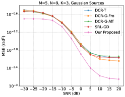
(a)

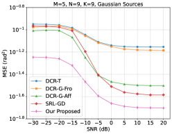
(b)

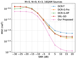
(c)

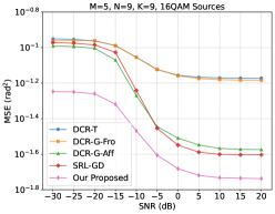
(d)

Figure 3: MSE as a function of SNR under both Gaussian and non-Gaussian signals with $M=5$ and $N=9$. The number of sources and signal types are listed in the title of each subfigure.

For the proposed Snap-TF, we set the attention activation dimension as $d_{\text{attn}}=96$, and adopt $L=2$ transformer layers for the Gaussian signals and $L=3$ layers in the case of non-Gaussian modulated symbols. After the transformer layers, we apply an affine mapping with a hidden dimension of 200 to transform the features to the estimated DOAs.

V-A3 Training Settings

We train the neural networks by using stochastic gradient descent (SGD) with a batch size of 4096. The models are trained for 100 epochs with the one-cycle scheduler of learning rates. For the benchmarks, we use the same learning rates as suggested in [31] (0.05 for DCR-T, 0.01 for DCR-G-Fro, 0.005 for DCR-G-Aff, and 0.1 for SRL-GD). For the proposed Snap-TF algorithm, we utilize a learning rate of 0.001. We generate $2\times 10^{6}$ training, $6\times 10^{4}$ validation, and $1\times 10^{4}$ testing samples, respectively. We use PyTorch to train and test all the models on one Nvidia A40 GPU.

V-B Performance

In Fig. 3, we plot the MSE of DOA estimation versus SNR for $M=5$ and $N=9$ under both Gaussian (the top panel) and non-Gaussian modulated sources (the bottom panel) with the number of sources $K=3,9$ arranged from left to right. These respectively represent cases where the number of sources is smaller and larger than the number of antennas. The model is trained over a mixture of SNR levels drawn uniformly from $[-20,20]$ dB, while tested in an SNR range of $[-30,20]$ dB.

First, the MSE of all methods decreases almost monotonically as the SNR increases. Our proposed Snap-TF algorithm always achieves the lowest error across the entire SNR range. Moreover, the performance gain is larger in the low-SNR regime. Second, comparing Gaussian versus non-Gaussian modulated (16QAM) signals, i.e., top vs. bottom in each column, the gap between Snap-TF and the benchmarks is larger for modulated sources. Snap-TF can leverage higher-order statistics of modulated symbols to localize better than covariance-based methods. These results show that the proposed Snap-TF algorithm can localize the uplink DOAs solely based on the unknown uplink data symbols, which is performed at the same time with data transmission, without additional overhead.

Third, increasing the number of sources from $K=3$ to $K=9$ raises the MSE for all methods, since $K=3$ (smaller than $M-1$) falls within the physical array’s degree of freedom while $K=9$ (larger than $M-1$) require exploiting the virtual array to resolve the sources. In both cases, Snap-TF consistently delivers better DOA estimation accuracy than all the benchmark methods. The extended localization capability is particularly useful for dense 6G networks with an ever-increasing number of sources that can greatly exceed the number of physical antennas, such as low-altitude UAV swarms which have immediate commercial values and are mentioned in discussions for 3GPP release 20 [6].

V-C Generalization Capability

In Fig. 4, we show the generalization capability of the proposed Snap-TF algorithms to practical mismatches, including the number of snapshots $T$ and the minimum angle separation $\Delta_{\bm{\theta},\min}$. All the methods shown in the figure are trained under $T=50$ and $\Delta_{\bm{\theta},\min}=\frac{\pi}{60}$, and directly tested in different cases. During testing, the received SNR is 10 dB, and the sources transmit 16QAM signals. As shown in the figure, the Snap-TF algorithm remains remarkably robust and consistently outperforms the benchmarks in terms of generalization performance.

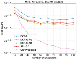
(a)

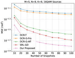
(b)

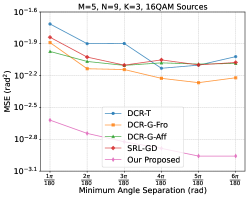
(c)

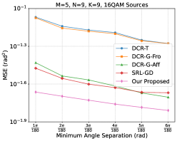
(d)

Figure 4: Generalization performance to different numbers of snapshots $T$ and minimum angle separations $\Delta_{\bm{\theta},\min}$. The model is trained under $T=50$ and $\Delta_{\bm{\theta},\min}=\frac{\pi}{60}$, and directly tested in all the different settings.

In the top panel, we evaluate the generalization performance across different snapshot counts $T$ ranging from 10 to 100, maintaining a fixed minimum angle separation of $\Delta_{\bm{\theta},\min}=\frac{\pi}{60}$. Our Snap-TF algorithm demonstrates exceptional robustness across this range. Despite training at $T=50$, Snap-TF exhibits remarkable generalization when operating with fewer snapshots ($T<50$) and continues to achieve superior performance gains as snapshot count increases ($T>50$), consistently outperforming all benchmark methods across the entire range. This outstanding generalization capability highlights a key strength of Snap-TF architecture, i.e., their inherent ability to adapt to varying snapshot counts while maintaining robust performance.

In the bottom panel, we evaluate generalization performance across varying minimum angle separations, testing $\Delta_{\bm{\theta},\min}$ values from $\frac{\pi}{180}$ (challenging closely spaced sources) to $\frac{6\pi}{180}$ (separated sources) at a fixed $T=50$. As expected, the DOA estimation task becomes increasingly difficult as $\Delta_{\bm{\theta},\min}$ decreases, presenting a natural challenge for all methods. Our Snap-TF algorithm excels across the entire range of $\Delta_{\bm{\theta},\min}$, consistently delivering the lowest MSE, including the challenging closely spaced scenarios.

V-D Scalability

In Fig. 5, we plot MSE-SNR curves to show that the proposed Snap-TF algorithm is scalable for large-scale MIMO systems. In this set of experiments, we adopt a 15-element MRA with $M=15$, which corresponds to a virtual ULA of $N=79$ elements, as introduced in Section V-A1. We consider the cases where the numbers of sources are $K=5$ and $K=20$, respectively. Other system settings are the same as described in Section V-A1. In this case, the benchmark methods will suffer from computational issues. The Root-MUSIC algorithm in the inference process requires the eigen-decomposition of an $N\times N$ complex-valued matrix, which is challenging to compute. In addition, the training process of the benchmarks DCR-G-Aff and SRL-GD both requires matrix inversion or decomposition to compute the loss function, which also undermines the scalability of their training process. In view of the complexity issue, we only compare with the most competitive benchmark, i.e., the SRL-GD algorithm, in the simulations.

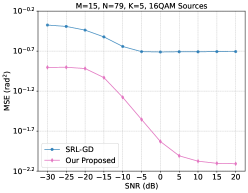
(a)

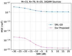
(b)

Figure 5: Scalability of the proposed Snap-TF algorithm in large-scale systems.

As shown, the proposed Snap-TF algorithm significantly outperforms the benchmark both when the number of sources $K$ is below the number of physical antennas ($K=5$) and when it exceeds it ($K=20$). The performance margin is even larger compared to that in the small-scale system. The results verify the scalability of the proposed algorithm in large-scale systems, and demonstrate its capability to localize more sources than antennas with unknown data symbols. The proposed algorithm also has significant advantages in complexity in large-scale systems, as will be detailed later.

V-E Complexity

In Fig. 6, we compare the complexity of different algorithms under various system scales including both runtime and number of trainable parameters. The runtime and number of parameters of the benchmarks are almost the same since they all use the same WRN network as backbone followed by the Root-MUSIC algorithm. We use SRL-GD as an indicator. The comparison is performed under 16QAM symbols, in which case we adopt 3 layers for the proposed Snap-TF algorithm.

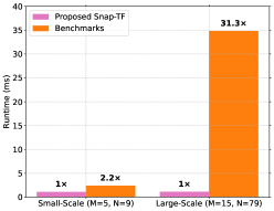
(a)

(b)

Figure 6: Comparison of complexity, including (a) runtime and (b) number of trainable parameters, under different system scales.

As seen in Fig. 6(a), the proposed Snap-TF algorithm consistently achieves sub-millisecond level runtime under both system configurations, approximately 1.103 ms for the small-scale case ($M=5$, $N=9$) and 1.112 ms for the large-scale case ($M=15$, $N=79$). By contrast, the benchmark DL-based subspace methods, which rely on matrix decompositions, exhibit a $2.2\times$ slowdown over Snap-TF in the small-scale case but suffer a dramatic $31.3\times$ increase in runtime when scaled up. This disparity underscores the heavy cost of the benchmarks, including $O(N^{3})$ operations such as matrix decomposition and inversion, making them computationally prohibitive in large-scale MIMO systems. By contrast, Snap-TF circumvents this bottleneck by eliminating the need for explicit matrix decomposition. It maintains a moderate runtime even in large-scale setups, and is suitable for real-time applications.

In Fig. 6(b), we compare the number of trainable parameters. The number for the benchmark is around 11 million and 17 million in the small-scale and large-scale setups, respectively, while that of the proposed Snap-TF algorithm (with 3 layers) is around 0.356 million in both setups. The proposed algorithm is $31.1\times$ and $49.7\times$ more efficient in parameters, respectively, which is lightweight for practical deployment.

V-F Ablation Studies

We conduct ablation studies to demonstrate Snap-TF’s capability to effectively learn and exploit higher-order statistical for DOA estimation. In the case of Gaussian signals, $k=2$ (second) order statistics are the sufficient statistics. As discussed in Section IV, only $L=\text{$\lceil\log_{2}(k+1)\rceil$}=2$ single-head transformer layers are sufficient. This is verified by the simulation results in Fig. 7(a), where we observe the performance starts to saturate when the model uses more than two layers. The saturation behavior provides evidence that Snap-TF has successfully captured all the relevant statistical information available in the Gaussian case, with additional layers offering diminishing returns. Similarly, in the non-Gaussian case, 16QAM symbols have non-zero $k=4$ (fourth) order cumulants [33], and hence $L=\text{$\lceil\log_{2}(k+1)\rceil$}=3$ layers are required. The results in Fig. 7(b) verify our hypothesis, which show that the performance keeps improving in the first three layers, and saturates thereafter. The performance pattern matches our prediction, and confirms that Snap-TF effectively captures the higher-order statistics required for non-Gaussian DOA estimation. This also suggests a lightweight 3-layer model is sufficient for pilot-free ISAC in cellular systems based on unknown uplink data symbols. We also label the number of parameters in the unit of million in the legends.

(a)

(b)

Figure 7: Ablation studies for the required layers of Snap-TF model.

VI Further Application: Sensing-Assisted MU-MIMO Beam Management

Beam sweeping is an important step of beam management to establish initial alignment. In the downlink, the BS will transmit synchronization signal blocks sequentially across various spatial directions, effectively “sweeping” its coverage range. The users then feedback the index of the strongest beams they receive to the BS to facilitate beam alignment. In the beam sweeping stage, the BS needs to sweep its whole coverage range based on a pre-defined codebook, for which a widely used choice is the discrete Fourier transform (DFT) codebook. Advanced codebook design has also been extensively studied to reduce the beam sweeping overhead and improve the performance.

However, it is less explored how to prune the beam sweeping range from the whole coverage area to a much smaller region during regular data transmission. This is what we hope to achieve through the sensing-assisted beam training. Thanks to the angular reciprocity, the uplink DOAs and the downlink DOAs are very close even in frequency division duplex (FDD) MU-MIMO systems [49, 37]. In the last section, we have shown that the proposed Snap-TF algorithm can accurately localize the DOAs of multiple sources based on the unknown uplink data symbols. These DOAs can help significantly narrow down the beam sweeping candidates without additional overhead. Importantly, while we will employ naive sweeping in the following experiments for illustrative purposes, sensing-assisted beam sweeping is fully compatible with any advanced beam sweeping codebook or algorithm in the literature. The sensed DOAs help greatly reduce the search space and provides a better initialization, making it a complementary enhancement for existing techniques.

VI-A Procedures

To show the capability of our sensing-assisted beam training to both reduce the beam sweeping overhead and improve the system throughput, we perform simulations in MU-MIMO systems. The number of snapshots for DOA estimation is set as $T=100$. We consider two cases where the SNR is set as -5 dB and 5 dB in the DOA estimation stage using unknown uplink data symbols. In the downlink transmission stage, we set the SNR as 10 dB. The $Q$ sweeping beams are chosen from a codebook $\mathcal{W}=\{\mathbf{w}_{q}=\mathbf{a}_{\bm{\Omega}}(\vartheta_{q})\}_{q=1}^{Q}$, in which $\vartheta_{q}=\sin^{-1}(\frac{2q}{Q}-1)$ with $q\in\{1,2,\ldots,Q\}$, according to Type I codebook [50]. We set the number of beam candidates as $Q=M$. Upon receiving the sweeping beams, each user will feedback its strongest beam index to the BS. The coherence interval, beam training overhead, and the feedback overhead are denoted by $T_{\text{c}}$, $T_{\text{train}}$, and $T_{\text{fb}}$ symbols, respectively.We evaluate the performance under $M=N=64$ with index set $\bm{\Omega}=\{1,2,3,\ldots,64\}$ and consider $K=10$ sources. The other parameters are the same as Section V-A. We compare the following methods to show the advantages of sensing-assisted beam management.

• Codebook only (full sweeping): The BS transmits over each of the $M$ codebook beams in sequence. All $K$ users measure these $M$ pilot transmissions, record the strongest beam index, and feed back to the BS. The beam sweeping overhead is $T_{\text{train}}=M$ symbols, and the feedback overhead is $T_{\text{fb}}=K$ symbols.

• Codebook + sensing (pruned sweeping): For the $k$-th user, only those candidate beams in the codebook $\mathbf{w}_{m}$ whose steering angles satisfy $|\vartheta_{m}-\hat{\theta}_{k}|<\delta,\forall m$ are sounded, where $\hat{\theta}_{k}$ denotes the estimated uplink DOA of the $k$-th user. Here, $\delta$ is the width of the search window that can be freely configured. We set $\delta$ as twice of the root MSE of the uplink DOA estimation. In this process, many beam candidates can be pruned away. Denote $\mathcal{W}_{k}\subseteq\mathcal{W}$ as the set of beams for the $k$-th user after pruning. The beam sweeping overhead is $T_{\text{train}}=|\bigcup_{k=1}^{K}\mathcal{W}_{k}|\leq M$ symbols, where $\bigcup$ denotes the union of sets, and the feedback overhead is $T_{\text{fb}}=K$ symbols.

• Sensing only (no sweeping): The BS directly reuses the estimated uplink DOA $\hat{\theta}_{k}$ as the beam direction for the $k$-th user without beam sweeping and feedback. The overheads are $T_{\text{train}}=T_{\text{fb}}=0$ symbols.

  

  Figure 8: Schematic diagram of three beam training schemes, i.e., codebook only (full sweeping), codebook + sensing (pruned sweeping), and sensing only (no sweeping). The dashed lines in the figure denote the estimated uplink DOAs, while the black triangles denote the BSs.

In Fig. 8, we draw diagrams of these schemes. After beam sweeping, the BS sends a small number pilots along the selected beam directions to estimate the channel gains by the least squares (LS) algorithm. Then, zero-forcing (ZF) precoding is adopted for downlink transmission. Similar to [37], we compare the system throughput, denoted by $R=\Bigl{(}1-\frac{T_{\mathrm{train}}+T_{\mathrm{fb}}}{T_{c}}\Bigr{)}\sum_{k=1}^{K}\log_{2}\bigl{(}1+\mathrm{SINR}_{k}\bigr{)}$, where $\text{SINR}_{k}$ is the signal-to-interference-plus-noise ratio of the $k$-th user.

VI-B Performance

Fig. 9 illustrates the system throughput as a function of the channel coherence time $T_{\text{c}}$ for three beam sweeping strategies. In Fig. 9 (a) and (b), DOA estimation from unknown uplink data symbols is performed at SNRs of -5 dB and 5 dB, respectively. Each data point in the plot is averaged over 10,000 Monte Carlo trials. The proposed codebook + sensing (pruned sweeping) approach consistently outperforms the conventional codebook-only method across all coherence time lengths, with the most pronounced advantage in the short coherence regime. This gain is attributed to the significant reduction of beam sweeping candidates enabled by the sensed uplink DOAs, which effectively lowers training overhead. The beam sweeping overhead for full sweeping is $T_{\text{train}}=64$, while the overhead of sensing pruned sweeping is significantly smaller, only leading to an average sweeping overhead of $T_{\text{train}}=5.0$ in (a) and $T_{\text{train}}=2.9$ in (b), which are respectively $12.8\times$ and $22.1\times$ times fewer compared to full sweeping. As the coherence interval $T_{\text{c}}$ increases, the performance of the full sweeping baseline gradually converges toward that of the proposed sensing-aided pruned sweeping scheme.

Comparing the sensing-only (no sweeping) method in both subfigures, we observe that in the low-SNR case, i.e., Fig. 9(a), the larger DOA estimation error renders direct reuse of the uplink DOAs for downlink transmission infeasible, whereas in the mid-SNR case, i.e., Fig. 9(b), the reduced estimation error yields better performance for downlink transmission. Although the sensing-only scheme eliminates beam sweeping overhead, its performance is highly sensitive to the DOA estimation accuracy. By contrast, the codebook + sensing (pruned sweeping) scheme is much more robust, delivering consistently competitive performance in both the low-SNR (a) and mid-SNR (b) cases. This demonstrates that even under low SNR, the DOA estimates are accurate enough to prune away a large number of beam candidates for downlink beam sweeping and achieve much higher system throughput. This demonstrates the value of the “sensing for free” paradigm and the effectiveness of the proposed algorithms for improving the communications performance.

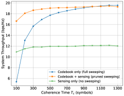
(a)

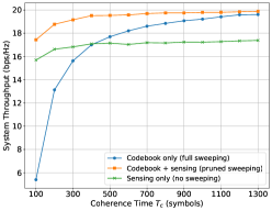
(b)

Figure 9: System throughput as a function of the coherence time $T_{\text{c}}$ for different beam sweeping schemes.

Importantly, the proposed sensing-assisted beam sweeping approach works seamlessly with existing 3GPP 5G NR standards and can be easily integrated into future 6G systems without requiring additional signaling overhead or changes to frame structures and waveforms. The pilot-free sensing leverages existing uplink data symbols that are part of the standard transmission protocol, making deployment straightforward within current and future cellular networks.

VII Conclusion

This paper demonstrates the novel paradigm of “sensing for free”—enabling multi-source localization at the BS based on unknown uplink data symbols, without dedicated pilots or additional overhead. Sparse arrays prove particularly promising for this paradigm, as they have the potential to localize more sources than antennas by exploiting their enlarged virtual array. Our attention-only transformer directly processes raw signal snapshots to exploit higher-order statistics for grid-less end-to-end multi-source DOA estimation, circumventing the computational bottlenecks and performance degradation inherent in existing DL-based subspace methods. These accurate DOA estimates can enable significant pruning of downlink beam sweeping candidates, and hence substantially reduce beam training overhead and enhance system throughput at no extra cost. By leaving frame structures and waveforms untouched, the paradigm integrates seamlessly into existing wireless systems and provides inspiration for next-generation 3GPP standardization efforts. Overall, this work reveals how uplink data symbols can be harnessed for free to unlock the substantial sensing capabilities, motivating future research into the untapped potential of regular data symbols for ISAC.

References

- [1] F. Liu, Y. Cui, C. Masouros, J. Xu, T. X. Han, Y. C. Eldar, and S. Buzzi, “Integrated sensing and communications: Toward dual-functional wireless networks for 6G and beyond,” IEEE J. Sel. Areas Commun., vol. 40, no. 6, pp. 1728–1767, Jun. 2022.
- [2] “Framework and overall objectives of the future development of imt for 2030 and beyond,” International Telecommunication Union Radiocommunication Sector (ITU-R), Tech. Rep. Recommendation ITU-R M.2160, November 2023, accessed: 2025-06-04. [Online]. Available: https://www.itu.int/rec/R-REC-M.2160-0-202311-I/en
- [3] 5G Americas, “ITU’s IMT-2030 vision: Navigating towards 6G in the Americas,” https://www.5gamericas.org/wp-content/uploads/2024/08/ITUs-IMT-2030-Vision_Id.pdf, 2024, accessed: 2025-06-04.
- [4] 3rd Generation Partnership Project (3GPP), “Study on Integrated Sensing and Communication,” 3GPP, Technical Report TR 22.837 V19.4.0, June 2024, release 19. [Online]. Available: https://www.3gpp.org/dynareport/22837.htm
- [5] W. Chen, X. Lin, J. Lee, A. Toskala, S. Sun, C. F. Chiasserini, and L. Liu, “5G-advanced toward 6G: Past, present, and future,” IEEE J. Sel. Areas Commun., vol. 41, no. 6, pp. 1592–1619, Jun. 2023.
- [6] X. Lin, “A tale of two mobile generations: 5G-advanced and 6G in 3GPP release 20,” arXiv preprint arXiv:2506.11828, Jun. 2025.
- [7] D. C. Nguyen, M. Ding, P. N. Pathirana, A. Seneviratne, J. Li, D. Niyato, O. Dobre, and H. V. Poor, “6G internet of things: A comprehensive survey,” IEEE Internet Things J., vol. 9, no. 1, pp. 359–383, Jan. 2022.
- [8] Y. Zeng, R. Zhang, and T. J. Lim, “Wireless communications with unmanned aerial vehicles: opportunities and challenges,” IEEE Comm. Mag., vol. 54, no. 5, pp. 36–42, May 2016.
- [9] Y. Jiang, X. Li, G. Zhu, H. Li, J. Deng, K. Han, C. Shen, Q. Shi, and R. Zhang, “Integrated sensing and communication for low altitude economy: Opportunities and challenges,” IEEE Commun. Mag., pp. 1–7, early access, 2025.
- [10] R. Schmidt, “Multiple emitter location and signal parameter estimation,” IEEE Trans. Antennas Propag., vol. 34, no. 3, pp. 276–280, Mar. 1986.
- [11] P. Pal and P. P. Vaidyanathan, “Nested arrays: A novel approach to array processing with enhanced degrees of freedom,” IEEE Trans. Signal Process., vol. 58, no. 8, pp. 4167–4181, Aug. 2010.
- [12] P. P. Vaidyanathan and P. Pal, “Sparse sensing with co-prime samplers and arrays,” IEEE Trans. Signal Process., vol. 59, no. 2, pp. 573–586, Feb. 2011.
- [13] A. Moffet, “Minimum-redundancy linear arrays,” IEEE Trans. Antennas Propag., vol. 16, no. 2, pp. 172–175, Mar. 1968.
- [14] X. Li, M. Jin, X.-T. Meng, B.-X. Cao, F.-G. Yan, M. S. Greco, and F. Gini, “Sparse linear arrays for direction-of-arrival estimation: A tutorial overview,” IEEE Aerosp. Electron. Syst. Mag., pp. 1–25, early access, 2025.
- [15] X. Li, H. Min, Y. Zeng, S. Jin, L. Dai, Y. Yuan, and R. Zhang, “Sparse MIMO for ISAC: New opportunities and challenges,” IEEE Wireless Commun., pp. 1–9, early access, 2025.
- [16] H. Min, X. Li, R. Li, and Y. Zeng, “Integrated localization and communication with sparse MIMO: Will virtual array technology also benefit wireless communication?” arXiv preprint arXiv:2502.18241, Feb. 2025.
- [17] H. Wang and Y. Zeng, “Can sparse arrays outperform collocated arrays for future wireless communications?” in Proc. IEEE Glob. Commun. Conf. Wkshps, Kuala Lumpur, Malaysia, Dec. 2023, pp. 667–672.
- [18] C. Zhou, C. You, H. Zhang, L. Chen, and S. Shi, “Sparse array enabled near-field communications: Beam pattern analysis and hybrid beamforming design,” arXiv preprint arXiv:2401.05690, Jan. 2024.
- [19] K. Chen, C. Qi, G. Y. Li, and O. A. Dobre, “Near-field multiuser communications based on sparse arrays,” IEEE J. Sel. Topics Signal Process., vol. 18, no. 4, pp. 619–632, May 2024.
- [20] A. Molisch and M. Win, “MIMO systems with antenna selection,” IEEE Microwave Mag., vol. 5, no. 1, pp. 46–56, Mar. 2004.
- [21] J. Zhang, X. Yu, and K. B. Letaief, “Hybrid beamforming for 5G and beyond millimeter-wave systems: A holistic view,” IEEE Open J. Commun. Soc., vol. 1, pp. 77–91, Jan. 2020.
- [22] K.-K. Wong, A. Shojaeifard, K.-F. Tong, and Y. Zhang, “Fluid antenna systems,” IEEE Trans. Wireless Commun., vol. 20, no. 3, pp. 1950–1962, Mar. 2021.
- [23] L. Zhu, W. Ma, and R. Zhang, “Modeling and performance analysis for movable antenna enabled wireless communications,” IEEE Trans. Wireless Commun., vol. 23, no. 6, pp. 6234–6250, Jun. 2024.
- [24] A. Barabell, “Improving the resolution performance of eigenstructure-based direction-finding algorithms,” in Proc. IEEE Int. Conf. Acoust. Speech Signal Process., vol. 8, Apr. 1983.
- [25] Z. Yang, L. Xie, and C. Zhang, “A discretization-free sparse and parametric approach for linear array signal processing,” IEEE Trans Signal Process., vol. 62, no. 19, pp. 4959–4973, Oct. 2014.
- [26] Y. Li and Y. Chi, “Off-the-grid line spectrum denoising and estimation with multiple measurement vectors,” IEEE Trans. Signal Process., vol. 64, no. 5, pp. 1257–1269, Mar. 2016.
- [27] G. Tang, B. N. Bhaskar, and B. Recht, “Near minimax line spectral estimation,” IEEE Trans. Inf. Theory, vol. 61, no. 1, pp. 499–512, Jan. 2015.
- [28] M. Wang, Z. Zhang, and A. Nehorai, “Grid-less DOA estimation using sparse linear arrays based on wasserstein distance,” IEEE Signal Process. Lett., vol. 26, no. 6, pp. 838–842, Jun. 2019.
- [29] A. Barthelme and W. Utschick, “DoA estimation using neural network-based covariance matrix reconstruction,” IEEE Signal Process. Lett., vol. 28, pp. 783–787, Apr. 2021.
- [30] X. Wu, X. Yang, X. Jia, and F. Tian, “A gridless DOA estimation method based on convolutional neural network with Toeplitz prior,” IEEE Signal Process. Lett., vol. 29, pp. 1247–1251, May 2022.
- [31] K.-L. Chen and B. D. Rao, “Subspace representation learning for sparse linear arrays to localize more sources than sensors: A deep learning methodology,” IEEE Trans. Signal Process., vol. 73, pp. 1293–1308, Feb. 2025.
- [32] A. Bjorck and G. H. Golub, “Numerical methods for computing angles between linear subspaces,” Math. Comp., vol. 27, no. 123, pp. 579–594, Jul. 1973.
- [33] N. Yuen and B. Friedlander, “DOA estimation in multipath: an approach using fourth-order cumulants,” IEEE Trans. Signal Process., vol. 45, no. 5, pp. 1253–1263, May 1997.
- [34] W. Peng, P. Li, X. Wu, K. Luo, G. Zheng, and D. Li, “Under-determined DOA estimation: A method based on higher-order statistics and non-uniform arrays,” IEEE Trans. Wireless Commun., vol. 23, no. 11, pp. 15 903–15 914, Nov. 2024.
- [35] K. Hugl, K. Kalliola, and J. Laurila, “Spatial reciprocity of uplink and downlink radio channels in FDD systems,” in Proc. COST, vol. 273, no. 2, Espoo, Finland, May 2002.
- [36] S. Imtiaz, G. S. Dahman, F. Rusek, and F. Tufvesson, “On the directional reciprocity of uplink and downlink channels in frequency division duplex systems,” in Proc. IEEE Int. Symp. Pers. Indoor and Mob. Radio Commun., Washington, DC, USA, Sept. 2014, pp. 172–176.
- [37] X. Zhang, L. Zhong, and A. Sabharwal, “Directional training for FDD massive MIMO,” IEEE Trans. Wireless Commun., vol. 17, no. 8, pp. 5183–5197, Aug. 2018.
- [38] M. Alrabeiah, A. Hredzak, and A. Alkhateeb, “Millimeter wave base stations with cameras: Vision-aided beam and blockage prediction,” in Prof. IEEE Veh. Technol. Conf., Antwerp, Belgium, May 2020, pp. 1–5.
- [39] G. Charan, T. Osman, A. Hredzak, N. Thawdar, and A. Alkhateeb, “Vision-position multi-modal beam prediction using real millimeter wave datasets,” in Proc. IEEE Wireless Commun. Netw. Conf., Austin, TX, USA, Apr. 2022, pp. 2727–2731.
- [40] K. Zhang, W. Yu, H. He, S. Song, J. Zhang, and K. B. Letaief, “Multimodal deep learning-empowered beam prediction in future THz ISAC systems,” in Proc. IEEE Int. Symp. Pers. Indoor and Mob. Radio Commun., Istanbul, Turkey, Sept. 2025.
- [41] W. Yu, Y. Shen, H. He, X. Yu, S. Song, J. Zhang, and K. B. Letaief, “An adaptive and robust deep learning framework for THz ultra-massive MIMO channel estimation,” IEEE J. Sel. Topics Signal Process., vol. 17, no. 4, pp. 761–776, Jul. 2023.
- [42] G. H. Hardy, J. E. Littlewood, and G. Pólya, Inequalities. Cambridge university press, 1934.
- [43] F. Schwartau, Y. Schröder, L. Wolf, and J. Schoebel, “Large minimum redundancy linear arrays: Systematic search of perfect and optimal rulers exploiting parallel processing,” IEEE Open J. Antennas Propagat., vol. 2, pp. 79–85, Jan. 2021.
- [44] P. Chevalier, L. Albera, A. Ferréol, and P. Comon, “On the virtual array concept for higher order array processing,” IEEE Trans. Signal Process., vol. 53, no. 4, pp. 1254–1271, Apr. 2005.
- [45] A. Vaswani, N. Shazeer, N. Parmar, J. Uszkoreit, L. Jones, A. N. Gomez, Ł. Kaiser, and I. Polosukhin, “Attention is all you need,” Adv. Neural Inf. Process. Syst., vol. 30, Dec. 2017.
- [46] J. L. Ba, J. R. Kiros, and G. E. Hinton, “Layer normalization,” arXiv preprint arXiv:1607.06450, Jul. 2016.
- [47] K. He, X. Zhang, S. Ren, and J. Sun, “Deep residual learning for image recognition,” in Proc. IEEE Conf. Comput. Vis. Pattern Recognit., Las Vegas, NV, USA 2016, pp. 770–778.
- [48] S. Wang, B. Z. Li, M. Khabsa, H. Fang, and H. Ma, “Linformer: Self-attention with linear complexity,” arXiv preprint arXiv:2006.04768, Jun. 2020.
- [49] H. Xie, F. Gao, S. Jin, J. Fang, and Y.-C. Liang, “Channel estimation for TDD/FDD massive MIMO systems with channel covariance computing,” IEEE Trans. Wireless Commun., vol. 17, no. 6, pp. 4206–4218, Jun. 2018.
- [50] E. Dahlman, S. Parkvall, and J. Skold, 5G NR: The next generation wireless access technology. Academic Press, 2020.