Neural Langevin Machine: a local asymmetric learning rule can be creative

Abstract

Fixed points of recurrent neural networks can be leveraged to store and generate information. These fixed points can be captured by the Boltzmann-Gibbs measure, which leads to neural Langevin dynamics that can be used for sampling and learning a real dataset. We call this type of generative model neural Langevin machine, which is interpretable thanks to its analytic form of distribution and is simple to train. Moreover, the learning process is derived as a local asymmetric plasticity rule, bearing biological relevance. Therefore, one can realize a continuous sampling of creative dynamics in a neural network, mimicking an imagination process in brain circuits. This neural Langevin machine may be another promising generative model, at least in its strength in circuit-based sampling and biologically plausible learning rule.

I Introduction

Generative models play an important role in modern machine learning, because of their wide applications in generating data samples after a complex non-analytic distribution is learned [1, 2, 3, 4]. These data samples cover a diverse range of high-dimensional vectors such as natural images, language texts, and even neural activities in the brain. Earlier representative energy-based generative models include restricted Boltzmann machine [1, 5], and recent neural-networks-based developments include variational auto-encoder [2], generative adversarial network [4], and a currently-dominant generative diffusion models [3, 6, 7]. In generative diffusion models, the forward stochastic dynamics and the backward score-driven stochastic dynamics are implemented [7]. The score is actually the gradient of the log-data-likelihood in the data space, approximated by a complex neural network that must be trained using the forward trajectories.

To mimic perception and imagination in brain dynamics, these artificial neural-network-based generative models are criticized to be lack of biological plausibility and are even complex in training with a bag of tricks. First, biological neural networks bear a recurrent structure that implements asymmetric learning rules [8, 9, 10]. Currently, popular generative models miss this biological setting. Second, the neural dynamics are used as a sampling machine, such as a probabilistic computation via neural response variability [11], and fixed points or chaotic attractors can be leveraged to store and generate examples [12]. Third, the learning is always local without a global artificial error signal in a biological circuit. Recent works have started to consider the role of chaotic activity in generating data samples [12]. However, the learning rule is still symmetric Hebbian type, despite a random asymmetric baseline considered. Moreover, there does not exist a potential landscape underlying the generative process. Another recent work proposed a Langevin dynamics with an Ising-type potential [13], but only the reverse trajectories are used to drive learning, which violates the above three biological relevance and thus does not pave a way towards understanding perception and imagination in the brain [14, 15].

In this work, we propose a neural Langevin machine (NLM) that satisfies the above three criteria. In particular, the generating process yields transitions among different types of data samples, resembling continuous brain dynamics driven by background stochastic noise. Hence, our work provides a promising avenue for neural-dynamics-based generative model that allows for a dynamic exploration of the creative activity space of imagination. In addition, the learning is simple and interpretable, derived from the kinetic energy landscape of recurrent neural dynamics (see a theoretical basis in our previous works [16, 17, 18, 19]).

II Neural Langevin machine as a generative model

The framework of quasi-potential dynamics offers an alternative perspective for constructing generative models. This approach involves minimizing the Kullback-Leibler (KL) divergence between the model’s equilibrium distribution and a target data distribution, thereby establishing a methodology analogous to the learning algorithms for Boltzmann machines [20].

Our previous work modified the chaotic recurrent neural network dynamics by introducing an Onsager feedback term to freeze the chaos [19]. This term is due to the minimization of the original kinetic energy (defined below) [16]. As we know, when the kinetic energy reaches zero, we get the set of fixed points of the original recurrent dynamics [21, 22], despite the fact that these fixed points are always unstable in the chaos phase. The Onsager feedback term is able to freeze chaos, which makes our following generative process theoretically-grounded. Inspired by these recent works, we can write an alternative neural dynamics:

$$\frac{d\mathbf{x}}{dt}=-\nabla_{\mathbf{x}}E(\mathbf{x})+\sqrt{2T}\bm{\epsilon}(t),$$ (1)

where $\mathbf{x}\in\mathbb{R}^{N}$ is the state vector. The potential (kinetic) energy function $E(\mathbf{x})$ is defined as:

$$E(\mathbf{x})=\frac{1}{2}\sum_{i=1}^{N}\left(-x_{i}+\sum_{j=1}^{N}J_{ij}\phi(x_{j})\right)^{2}.$$ (2)

In this paper, we set $\phi(x)=\tanh(x)$. Here $T$ represents a temperature parameter, and $\bm{\epsilon}(t)$ is an $N$-dimensional Gaussian white noise vector, characterized by zero mean $\langle\epsilon_{i}(t)\rangle=0$ and temporal correlation $\langle\epsilon_{i}(t)\epsilon_{j}(t^{\prime})\rangle=\delta_{ij}\delta(t-t^{\prime})$. $J_{ij}$ denotes the neural coupling from neuron $j$ to $i$. They are always asymmetric, thereby allowing for no potential function for the original chaotic neural dynamics (in the absence of the Onsager feedback term, see below).

The $i$-th component of the gradient force $-\nabla_{\mathbf{x}}E(\mathbf{x})$, denoted as $F_{i}$, is given by:

$$F_{i}\equiv-\frac{\partial E(\mathbf{x})}{\partial x_{i}}=-x_{i}+h_{i}-\phi^{\prime}(x_{i})\sum_{j=1}^{N}J_{ji}(h_{j}-x_{j}),$$ (3)

where we introduce the auxiliary variable as integrated synaptic current $h_{i}\equiv\sum_{j=1}^{N}J_{ij}\phi(x_{j})$, and $\phi^{\prime}(x_{i})$ denotes the derivative of $\phi(x_{i})$ with respect to $x_{i}$. The last term in the right-hand-side of Eq. (3) is the very Onsager feedback term, which plays an important role in stabilizing the chaotic fluctuations [19].

The system described by Eq. (1) converges to an equilibrium (stationary in the sense of Fokker-Planck equation) distribution, $P(\mathbf{x})$, which takes the form of a Boltzmann-Gibbs distribution [23]:

$$P(\mathbf{x})=\frac{1}{Z}\exp(-\beta E(\mathbf{x})),$$ (4)

where $\beta=1/T$ is the inverse temperature, and $Z=\int\exp(-\beta E(\mathbf{x}))d\mathbf{x}$ is the partition function, ensuring normalization. A statistical mechanics analysis of this partition function in a random recurrent neural network with or without learning has been done in recent works [16, 18].

Our objective is then to optimize the coupling parameters $\{J_{kl}\}$ such that the model distribution $P(\mathbf{x})$ closely approximates a given data distribution $P_{data}(\mathbf{x})$. The discrepancy between these two distributions is quantified by the Kullback-Leibler (KL) divergence:

$$\mathcal{L}_{KL}(P_{data}||P) =\int P_{data}(\mathbf{x})\ln\frac{P_{data}(\mathbf{x})}{P(\mathbf{x})}d\mathbf{x}$$ (5)

$$=\int P_{data}(\mathbf{x})\ln P_{data}(\mathbf{x})d\mathbf{x}-\int P_{data}(\mathbf{x})\ln P(\mathbf{x})d\mathbf{x}$$

$$=\int P_{data}(\mathbf{x})\ln P_{data}(\mathbf{x})d\mathbf{x}-\int P_{data}(\mathbf{x})\ln\left(\frac{1}{Z}\exp(-\beta E(\mathbf{x}))\right)d\mathbf{x}$$

$$=\int P_{data}(\mathbf{x})\ln P_{data}(\mathbf{x})d\mathbf{x}-\int P_{data}(\mathbf{x})(-\ln Z-\beta E(\mathbf{x}))d\mathbf{x}$$

$$=\langle\ln P_{data}(\mathbf{x})\rangle_{data}+\ln Z+\beta\langle E(\mathbf{x})\rangle_{data}.$$

Here, $\langle\cdot\rangle_{data}$ denotes an expectation taken with respect to $P_{data}(\mathbf{x})$. Since the term $\langle\ln P_{data}(\mathbf{x})\rangle_{data}$ is independent of the model parameters, minimizing $\mathcal{L}_{KL}$ is equivalent to minimizing the objective function $\mathcal{L}(\mathbf{J})=\ln Z+\beta\langle E(\mathbf{x})\rangle_{data}$. If we define $\ln Z$ as a negative free energy, this objective function bears the physical meaning of entropy in physics.

To perform gradient-based optimization, we compute the partial derivative of $\mathcal{L}_{KL}$ [or effectively $\mathcal{L}(\mathbf{J})$] with respect to a specific parameter $J_{kl}$:

$$\frac{\partial\mathcal{L}_{KL}}{\partial J_{kl}} =\frac{\partial}{\partial J_{kl}}\left(\ln Z+\beta\langle E(\mathbf{x})\rangle_{data}\right)$$ (6)

$$=\frac{1}{Z}\frac{\partial Z}{\partial J_{kl}}+\beta\left\langle\frac{\partial E(\mathbf{x})}{\partial J_{kl}}\right\rangle_{data}.$$

The derivative of the partition function is given by

$$\frac{\partial Z}{\partial J_{kl}} =\frac{\partial}{\partial J_{kl}}\int\exp(-\beta E(\mathbf{x}))d\mathbf{x}$$ (7)

$$=\int-\beta\frac{\partial E(\mathbf{x})}{\partial J_{kl}}\exp(-\beta E(\mathbf{x}))d\mathbf{x}.$$

Thus, the first term in Eq. (6) becomes:

$$\frac{1}{Z}\frac{\partial Z}{\partial J_{kl}}=-\beta\int\frac{\partial E(\mathbf{x})}{\partial J_{kl}}\frac{\exp(-\beta E(\mathbf{x}))}{Z}d\mathbf{x}=-\beta\left\langle\frac{\partial E(\mathbf{x})}{\partial J_{kl}}\right\rangle_{model},$$ (8)

where $\langle\cdot\rangle_{model}$ denotes an expectation taken with respect to the model distribution $P(\mathbf{x})$. Substituting this back into Eq. (6), we get:

$$\frac{\partial\mathcal{L}_{KL}}{\partial J_{kl}}=-\beta\left\langle\frac{\partial E(\mathbf{x})}{\partial J_{kl}}\right\rangle_{model}+\beta\left\langle\frac{\partial E(\mathbf{x})}{\partial J_{kl}}\right\rangle_{data}.$$ (9)

Equation (9) implies that when the two gradients of the Hamiltonian match with each other, the learning terminates.

Next, we need the derivative of the energy function $E(\mathbf{x})$ [from Eq. (2)] with respect to $J_{kl}$:

$$\frac{\partial E(\mathbf{x})}{\partial J_{kl}} =\frac{\partial}{\partial J_{kl}}\left[\frac{1}{2}\sum_{i=1}^{N}\left(-x_{i}+\sum_{m=1}^{N}J_{im}\phi(x_{m})\right)^{2}\right]$$ (10)

$$=\left(-x_{k}+\sum_{m=1}^{N}J_{km}\phi(x_{m})\right)\cdot\frac{\partial}{\partial J_{kl}}\left(\sum_{m=1}^{N}J_{km}\phi(x_{m})\right)$$

$$=\left(-x_{k}+\sum_{m=1}^{N}J_{km}\phi(x_{m})\right)\phi(x_{l})$$

$$=(-x_{k}+h_{k})\phi(x_{l}),$$

where $h_{k}=\sum_{m=1}^{N}J_{km}\phi(x_{m})$ is defined before.

Substituting Eq. (10) into Eq. (9), we obtain:

$$\frac{\partial\mathcal{L}_{KL}}{\partial J_{kl}} =-\beta\left\langle(-x_{k}+h_{k})\phi(x_{l})\right\rangle_{model}+\beta\left\langle(-x_{k}+h_{k})\phi(x_{l})\right\rangle_{data}$$ (11)

$$=\beta\left[\left\langle(x_{k}-h_{k})\phi(x_{l})\right\rangle_{model}-\left\langle(x_{k}-h_{k})\phi(x_{l})\right\rangle_{data}\right]$$

$$=\beta\left[\left\langle x_{k}\phi(x_{l})-h_{k}\phi(x_{l})\right\rangle_{model}-\left\langle x_{k}\phi(x_{l})-h_{k}\phi(x_{l})\right\rangle_{data}\right].$$

This is the final expression for the gradient of the KL divergence with respect to the parameter $J_{kl}$. Clearly, this is not of Hebbian type but of asymmetric one, which is a salient distinction from recent works [12].

To minimize the KL divergence, network parameters are updated iteratively using gradient descent:

$$(J_{kl})_{n+1} =(J_{kl})_{n}-\eta\frac{\partial\mathcal{L}_{KL}}{\partial J_{kl}}$$ (12)

$$=(J_{kl})_{n}-\eta\beta\left[\left\langle x_{k}\phi(x_{l})-h_{k}\phi(x_{l})\right\rangle_{model}-\left\langle x_{k}\phi(x_{l})-h_{k}\phi(x_{l})\right\rangle_{data}\right]$$

$$=(J_{kl})_{n}-\eta\beta\left\langle x_{k}\phi(x_{l})-h_{k}\phi(x_{l})\right\rangle_{model}+\eta\beta\left\langle x_{k}\phi(x_{l})-h_{k}\phi(x_{l})\right\rangle_{data},$$

where $\eta>0$ is the learning rate, and $(J_{kl})_{n}$ denotes the value of the parameter at iteration $n$. This update rule adjusts $J_{kl}$ to reduce the discrepancy between statistics computed from the model-generated samples (the model phase) and those computed from the training data (the data phase). The model phase can be estimated by running the Langevin dynamics and collected intermediate states as samples based on the current estimates of $\{J_{kl}\}$.

III Training protocol

The primary goal of the training process is to adjust the coupling parameters $\mathbf{J}$ of the quasi-potential model such that its equilibrium distribution $P(\mathbf{x})$ [Eq. (4)] closely approximates the target data distribution $P_{data}(\mathbf{x})$. This is achieved by minimizing the Kullback-Leibler (KL) divergence $\mathcal{L}_{KL}(P_{data}||P)$ [Eq. (5)] with respect to $\mathbf{J}$. The optimization is performed using stochastic gradient descent, where the gradient of the KL divergence with respect to a parameter $J_{kl}$ is given by Eq. (11):

$$\frac{\partial\mathcal{L}_{KL}}{\partial J_{kl}}=\beta\left[\left\langle(x_{k}-h_{k})\phi(x_{l})\right\rangle_{model}-\left\langle(x_{k}-h_{k})\phi(x_{l})\right\rangle_{data}\right],$$ (13)

where $h_{k}=\sum_{l=1}^{N}J_{kl}\phi(x_{l})$ and $\beta=1/T$. The evaluation of this gradient involves two expectation terms: one with respect to the model distribution $P(\mathbf{x})$ and the other with respect to the data distribution $P_{data}(\mathbf{x})$.

In the data phase, the expectation $\left\langle(x_{k}-h_{k})\phi(x_{l})\right\rangle_{data}$ is estimated empirically using a mini-batch of $m$ samples $\{\mathbf{x}^{(s)}\}_{s=1}^{m}$ drawn from the training dataset $\mathbf{X}_{data}$. For each sample $\mathbf{x}^{(s)}$ in the batch, we compute $h_{k}^{(s)}=\sum_{l}J_{kl}\phi(x_{l}^{(s)})$. The data-dependent term $A_{kl}$ in Alg. 1 (see Appendix) is estimated as

$$A_{kl}=\beta\cdot\frac{1}{m}\sum_{s=1}^{m}\left(x_{k}^{(s)}-\left(\mathbf{J}\tanh(\mathbf{x}^{(s)})\right)_{k}\right)\tanh(x_{l}^{(s)}),$$ (14)

where the notation $(\mathbf{v})_{k}$ denotes the $k$-th component of vector $\mathbf{v}$, i.e., $h_{k}^{(s)}$.

In the model phase, the expectation $\left\langle(x_{k}-h_{k})\phi(x_{l})\right\rangle_{model}$ is more challenging to compute as it requires sampling from the model’s Boltzmann-Gibbs distribution $P(\mathbf{x})$. This is achieved by simulating the Langevin dynamics described in Eq. (1). For practical implementation, the stochastic differential equation is discretized using an Euler-Maruyama scheme with a time step $dt$:

$$\mathbf{x}_{t+dt}=\mathbf{x}_{t}+dt\cdot{\bf{F}}(\mathbf{x}_{t})+\sqrt{2Tdt}\bm{\epsilon}_{t},$$ (15)

where $\mathbf{F}(\mathbf{x}_{t})=-\nabla_{\mathbf{x}}E(\mathbf{x}_{t})$ is the deterministic force vector with components $F_{i}$ given by Eq. (3), and $\bm{\epsilon}_{t}$ is a vector of independent standard Gaussian random variables. In matrix form for a set of states $\mathbf{X}_{t}$, the dynamics can thus be written as follows (used in Alg. 1):

$$\mathbf{X}_{t+dt}=(1-dt)\mathbf{X}_{t}+dt\cdot\mathbf{J}\tanh(\mathbf{X}_{t})-dt\cdot(\phi^{\prime}(\mathbf{X}_{t})\odot(\mathbf{J}^{\top}(\mathbf{J}\tanh(\mathbf{X}_{t})-\mathbf{X}_{t})))+\sqrt{2T\,dt}\,\bm{\mathcal{E}}_{t},$$ (16)

where $\odot$ denotes Hadamard product, $\phi^{\prime}(x)=1-\tanh^{2}(x)$, and $\bm{\mathcal{E}}_{t}$ is a matrix of i.i.d. Gaussian noise.

To improve the sampling efficiency and quality, $M$ persistent chains (model states $\mathbf{X}_{model}$) are created. These chains are initialized once (e.g., from a Gaussian distribution) and then updated by running the Langevin dynamics for $n_{t}$ steps. The final states of these chains after $n_{t}$ steps are used to estimate the model expectation. The term $B_{kl}$ in Alg. 1 represents this expectation, scaled by $\beta$:

$$B_{kl}=\beta\cdot\frac{1}{M}\sum_{s=1}^{M}\left(x_{k}^{(s)}-\left(\mathbf{J}\tanh(\mathbf{x}^{(s)})\right)_{k}\right)\tanh(x_{l}^{(s)}),$$ (17)

where $\{\mathbf{x}^{(s)}\}_{s=1}^{M}$ are the samples from all the persistent chains. This term approximates $\beta\left\langle(x_{k}-h_{k})\phi(x_{l})\right\rangle_{model}$. After each gradient calculation (learning), the final states of the chains serve as initial states for the next iteration.

With the data-dependent term $A_{kl}$ and model-dependent term $B_{kl}$ computed, the gradient of the KL divergence with respect to $J_{kl}$ is approximated by $(B_{kl}-A_{kl})$. The coupling parameters are then updated using gradient descent:

$$(J_{kl})_{new}=(J_{kl})_{old}-\eta(B_{kl}-A_{kl}),$$ (18)

where $\eta$ (see Alg. 1) is the learning rate. Additionally, a weight decay term with coefficient $\lambda_{1}$ is typically included in the optimization step to regularize the model and prevent overfitting. This corresponds to adding $\lambda_{1}J_{kl}$ to the above gradient term. The overall training procedure is sketched in Alg. 1. The process continues for a predefined number of epochs $n$, or until a convergence criterion is met.

IV Generation process

The generation process aims to draw samples from the learned model distribution $P(\mathbf{x})$. This is achieved by simulating the $N$-dimensional stochastic differential equation under the quasi-potential [Eq. (1)], using the final trained parameters $\mathbf{J}_{\text{final}}$ and the same temperature:

$$\frac{d\mathbf{x}}{dt}=-\nabla_{\mathbf{x}}E(\mathbf{x}|\mathbf{J}_{\text{final}})+\sqrt{2T}\bm{\epsilon}(t),$$ (19)

where $E(\mathbf{x}|\mathbf{J}_{\text{final}})$ explicitly denotes the energy function parameterized by the trained $\mathbf{J}_{\text{final}}$. The goal is to obtain samples $\mathbf{x}$ that are distributed according to $P(\mathbf{x})=\frac{1}{Z}\exp(-\beta E(\mathbf{x}|\mathbf{J}_{\text{final}}))$.

The simulation starts from a batch of initial states $\mathbf{X}_{0}\in\mathbb{R}^{N\times N_{gen}}$, each column of which is drawn independently from an isotropic Gaussian distribution $\mathcal{N}(\mathbf{0},\mathds{1}_{N})$. $N_{gen}$ denotes the total number of generated images. The Langevin dynamics are simulated numerically using the same Euler-Maruyama discretization scheme as employed during the model phase of training [derived from Eq. (15)]:

$$\mathbf{X}_{t+dt}=\mathbf{X}_{t}+dt\cdot{\bf{F}}(\mathbf{X}_{t}|\mathbf{J}_{\text{final}})+\sqrt{2Tdt}\bm{\mathcal{E}}_{t},$$ (20)

where ${\bf{F}}(\mathbf{X}_{t}|\mathbf{J}_{\text{final}})=-\nabla_{\mathbf{X}}E(\mathbf{X}_{t}|\mathbf{J}_{\text{final}})$ is the deterministic force vector evaluated with the trained parameters. The component-wise expression for the force $F_{i}$ is given by Eq. (3). When $\mathbf{X}_{t}$ is a matrix representing a batch of states (e.g., $\mathbf{X}_{t}\in\mathbb{R}^{N\times N_{gen}}$), the update rule can be written in matrix form as:

$$\mathbf{X}_{t+dt}=(1-dt)\mathbf{X}_{t}+dt\cdot\mathbf{J}_{\text{final}}\tanh(\mathbf{X}_{t})-dt\cdot(\phi^{\prime}(\mathbf{X}_{t})\odot(\mathbf{J}_{\text{final}}^{\top}(\mathbf{J}_{\text{final}}\tanh(\mathbf{X}_{t})-\mathbf{X}_{t})))+\sqrt{2T\,dt}\,\bm{\mathcal{E}}_{t},$$ (21)

where $\phi^{\prime}(x)=1-\tanh^{2}(x)$ is the derivative of $\phi(x)=\tanh(x)$, $\odot$ denotes the Hadamard (element-wise) product, and $\bm{\mathcal{E}}_{t}$ is a matrix of i.i.d. standard Gaussian random variables of the same dimension as $\mathbf{X}_{t}$. This simulation is run for a specified number of steps, $n_{t}$, which should be sufficiently large to allow the system to converge to (or draw representative samples from) its equilibrium distribution $P(\mathbf{x})$. After $n_{t}$ steps of simulation, the final state matrix $\mathbf{X}_{\text{final}}$ contains the generated samples, which is outlined in Alg.  2 (see Appendix).

As a proof of concept, we applied the learning scheme to the benchmark dataset of MNIST handwritten digits [24]. We plot a low-dimensional visualization of training and generated digits in Fig. 1, which shows how the generated images change as the neural dynamics are going on the kinetic energy landscape. The landscape acts as an attractive manifold, being the source of the creative ability of NLM. Evidences were found in the brain about how low-dimensional attractors are created during perception, memory and decision making [25]. The generative state transition is driven here by the stochastic noise (see Fig. 2). More generated examples of training images are shown in Fig. 3. Although this neural Langevin machine is simple to train, bearing biological relevance, and is also easy to understand, it is still necessary to improve the quality of generated samples, perhaps by virtue of considering hidden activity, plasticity modulation, etc. We leave this to a future work.

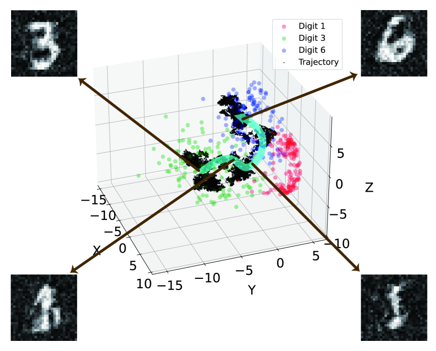
Figure 1: Principal Component Analysis (PCA) of learning results. Four hundred data points from the training set are considered, which consists of digits 1, 3, and 6, projected onto three-dimensional space. These principal components were then used as a basis to plot the trajectory of the sampling process. The visualization demonstrates transitions among generated images from digit 3, to digit 1, and finally to digit 6. In the training set, digits 1, 3, and 6 are indicated by red, green, and blue colors, respectively. The sampling trajectory, running from the $100$th second to the $250$th second, is marked by small black dots.

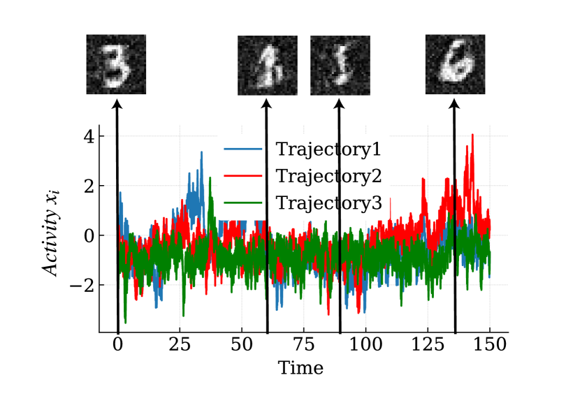
Figure 2: Trajectory of Langevin dynamics during digit generation corresponding to Fig. 1. Typical neural activity trajectories of three neurons are shown.

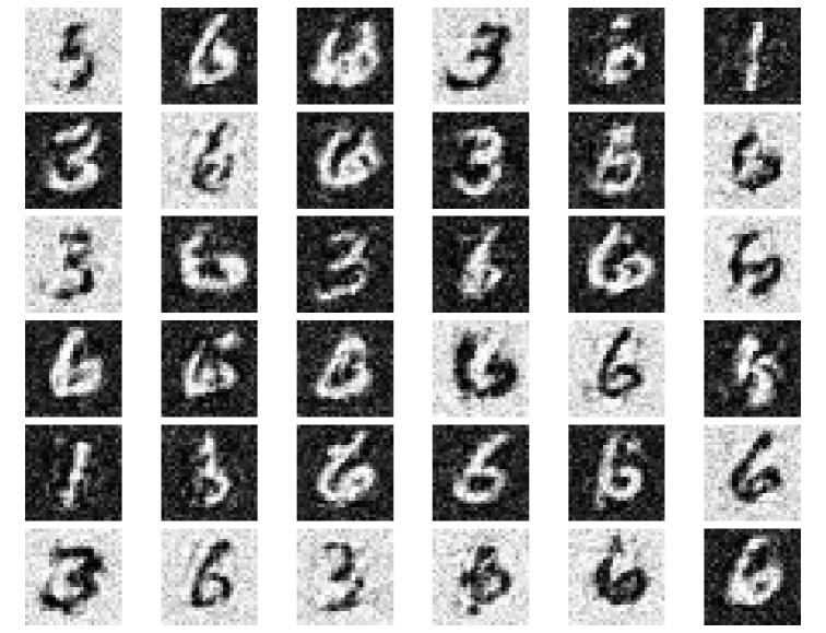
Figure 3: Training NLM with digits 1, 3, and 6. The generated images are shown for some examples. Each examples are drawn from the final state of independent dynamics trajectory.

V Conclusion and future remarks

In this work, we propose a neural Langevin machine that use stationary neural dynamics to store and generate data samples, establishing a strong link between theory of out-of-equilibrium fixed points [16, 19] and brain dynamics as a generative machine. Using NLM, we realize asymmetric local learning rules (beyond simple Hebbian-like plasticity rule) and state transition among metal novel images. We show a proof of this principle in the current work. Future exciting directions include an improvement of data quality in generated samples. To achieve this, several factors may be important. First, different time scales in both neural and synaptic dynamics must be considered. Second, layered recurrent structure may also be a key factor. Third, multiple forms of synaptic plasticity may be also necessary to enhance the quality of imagination, which can be inspired by the theory of hierarchically coupled dynamics [18, 26, 27]. We thus anticipate that this NLM will inspire further developments in the field of generative models, thereby guiding us to understand how we subjectively perceive and imagine the objective outside world.

Appendix A Algorithmic details of NLM

The pseudocode of the training process is given in Alg. 1. The pseudocode of the generation process is given in Alg. 2. Hyperparameters used in figures are specified in Table 1. Note that $M=m$ in our implementation of training the recurrent networks. Codes are available in our GitHub [28].

Algorithm 1 Training protocol of NLM

1:Hyperparameters: $N$: network size, $g$: initial coupling strength; $T$: temperature; $dt$: time increment; $n$: the number of epochs; $n_{t}$: the number of dynamic steps per coupling update; $\eta$: learning rate; $\lambda_{1}$: weight decay parameter; $m$: mini-batch size; $M$: the number of persistent chains; $N_{image}$: the number of training images.

2:Initialization:

3:Load MNIST dataset, preprocess it by applying a linear transformation to ${\bf{X}}_{data}\in\mathbb{R}^{N\times N_{image}}$ (values in $[-1,1]$).

4:Initialize $\mathbf{J}\in\mathbb{R}^{N\times N}$ (sampled from $\mathcal{N}(0,g^{2}/N)$, $J_{ii}=0$).

5:Initialize persistent model states $\mathbf{X}_{model}\in\mathbb{R}^{N\times M}$, where each entry $[\mathbf{X}_{model}]_{ij}\overset{\text{i.i.d.}}{\sim}\mathcal{N}(0,1)$.

6:Training Loop:

7:for epoch $=1$ to $n$ do

8:  for each batch ${\bf{X}}_{batch}$ from DataLoader(${\bf{X}}_{data}$) do

9:   Data average: Calculate

$$A=\frac{1}{T\cdot m}\left({\bf{X}}_{batch}-\mathbf{J}\tanh({\bf{X}}_{batch})\right)\tanh({\bf{X}}_{batch})^{\top}$$

10:   Model Sampling:

11:   Initial states ${\bf{X}}_{0}\leftarrow{\bf{X}}_{{model}}$

12:   Run quasi-potential dynamics for $n_{t}$ steps with step size $dt$:

13:   $\triangleright$ Dynamics: ${\bf{X}}_{t+dt}=(1-dt){\bf{X}}_{t}+dt\cdot\mathbf{h}_{t}-dt\cdot(\phi^{\prime}({\bf{X}}_{t})\odot\bm{\delta J}_{t})+\sqrt{2T\,dt}\,{\boldsymbol{\varepsilon}_{t}}$

14:   $\triangleright$ where $\mathbf{h}_{t}=\mathbf{J}\tanh({\bf{X}}_{t})$, $\bm{\delta J}_{t}=\mathbf{J}^{\top}(\mathbf{h}_{t}-{\bf{X}}_{t})$, $\phi^{\prime}(x)=1-\tanh^{2}(x)$, ${\boldsymbol{\varepsilon}_{t}}\sim{\cal N}(0,\mathds{1}_{N})$

15:   Update persistent states $\mathbf{X}_{model}\leftarrow$ final state of dynamics.

16:   Model average: Calculate

$$B=\frac{1}{T\cdot M}\left(\mathbf{X}_{\text{model}}-\mathbf{J}\tanh(\mathbf{X}_{\text{model}})\right)\tanh(\mathbf{X}_{\text{model}})^{\top}$$

17:   Update: Update $\mathbf{J}$ using gradient $(B-A)$ and weight decay $\lambda_{1}$.

18:  end for

19:end for

20:Store the final trained matrix $\mathbf{J}_{\text{final}}$.

Algorithm 2 Generation process

1:Hyperparameters: $N$: network size; $T$: temperature; $dt$: time increment; $n_{t}$: the number of steps; $N_{gen}$ : the number of generated samples.

2:Initialization: Load the previously stored $\mathbf{J}_{\text{final}}$. Initialize one or more states ${{\bf{X}}_{0}}\in\mathbb{R}^{N\times N_{gen}}$; for instance, each column is drawn from ${\cal N}(\mathbf{0},\mathds{1}_{N})$.

3:Generation process:

4:Set $\mathbf{J}\leftarrow\mathbf{J}_{\text{final}}$.

5:Run quasi-potential dynamics for $n_{t}$ steps with step size $dt$, starting from ${\bf{X}}_{0}$:

6:for $s=0$ to $n_{t}$ do

7:  $\mathbf{h}_{t}=\mathbf{J}\tanh({\bf{X}}_{t})$

8:  $\bm{\delta J}_{t}=\mathbf{J}^{\top}(\mathbf{h}_{t}-{\bf{X}}_{t})$

9:  $\phi^{\prime}(\mathbf{X}_{t})=1-\tanh^{2}(\mathbf{X}_{t})$ (element-wise)

10:  Generate $\bm{\mathcal{E}}_{t}\sim\mathcal{N}(\mathbf{0},\mathds{1}_{N})$ with the same dimension as $\mathbf{X}_{t}$.

11:  ${\bf{X}}_{t+dt}=(1-dt){\bf{X}}_{t}+dt\cdot\mathbf{h}_{t}-dt\cdot(\phi^{\prime}({\bf{X}}_{t})\odot\bm{\delta J}_{t})+\sqrt{2T\,dt}\,\bm{\mathcal{E}_{t}}$

12:end for

13:Let ${\bf{X}}_{\text{final}}\leftarrow$ finite state of the trajecory.

14:Store the final mapped states $\phi({{\bf{X}}_{\text{final}}})$ used to be transformed into generated images.

Table 1: Hyperparameters for figures in the main text

Figure	$g$	$N$	$dt$	$n_{t}$	$n$	$\eta$	$\lambda_{1}$	$T$	$m$	$N_{image}$
1	2	784	0.01	10	3000	0.0005	0.000002	1	1000	18000
2	2	784	0.01	10	3000	0.0005	0.000002	1	1000	18000
3	2	784	0.01	10	3000	0.0005	0.000002	1	1000	18000

References

- [1] Geoffrey E Hinton. Training products of experts by minimizing contrastive divergence. Neural computation, 14(8):1771–1800, 2002.
- [2] Diederik P. Kingma and Max Welling. An introduction to variational autoencoders. Foundations and Trends® in Machine Learning, 12(4):307–392, 2019.
- [3] Jascha Sohl-Dickstein, Eric Weiss, Niru Maheswaranathan, and Surya Ganguli. Deep unsupervised learning using nonequilibrium thermodynamics. In International conference on machine learning, pages 2256–2265. PMLR, 2015.
- [4] Ian J Goodfellow, Jean Pouget-Abadie, Mehdi Mirza, Bing Xu, David Warde-Farley, Sherjil Ozair, Aaron Courville, and Yoshua Bengio. Generative adversarial nets. Advances in neural information processing systems, pages 2672–2680, 2014.
- [5] Haiping Huang. Variational mean-field theory for training restricted boltzmann machines with binary synapses. Phys. Rev. E, 102:030301, Sep 2020.
- [6] Yang Song, Jascha Sohl-Dickstein, Diederik P Kingma, Abhishek Kumar, Stefano Ermon, and Ben Poole. Score-based generative modeling through stochastic differential equations. In International Conference on Learning Representations, 2021.
- [7] Zhendong Yu and Haiping Huang. Nonequilbrium physics of generative diffusion models. Phys. Rev. E, 111:014111, 2025.
- [8] Dean V. Buonomano and Wolfgang Maass. State-dependent computations: spatiotemporal processing in cortical networks. Nature Reviews Neuroscience, 10(2):113–125, 2009.
- [9] Wulfram Gerstner, Werner M. Kistler, Richard Naud, and Liam Paninski. Neuronal Dynamics: From Single Neurons to Networks and Models of Cognition. Cambridge University Press, United Kingdom, 2014.
- [10] Jeffrey C. Magee and Christine Grienberger. Synaptic plasticity forms and functions. Annual Review of Neuroscience, 43(Volume 43, 2020):95–117, 2020.
- [11] Patrik O. Hoyer and Aapo Hyvärinen. Interpreting neural response variability as monte carlo sampling of the posterior. In Proceedings of the 16th International Conference on Neural Information Processing Systems, NIPS’02, page 293–300, Cambridge, MA, USA, 2002. MIT Press.
- [12] Samantha J Fournier and Pierfrancesco Urbani. Generative modeling through internal high-dimensional chaotic activity. Physical Review E, 111(4):045304, 2025.
- [13] Stephen Whitelam. Generative thermodynamic computing. arXiv:2506.15121, 2025.
- [14] Mikhail I. Rabinovich, Pablo Varona, Allen I. Selverston, and Henry D. I. Abarbanel. Dynamical principles in neuroscience. Rev. Mod. Phys., 78:1213–1265, 2006.
- [15] Haiping Huang. Eight challenges in developing theory of intelligence. Front. Comput. Neurosci, 18:1388166, 2024.
- [16] Junbin Qiu and Haiping Huang. An optimization-based equilibrium measure describing fixed points of non-equilibrium dynamics: application to the edge of chaos. Communications in Theoretical Physics, 77(3):035601, 2025.
- [17] Shishe Wang and Haiping Huang. How high dimensional neural dynamics are confined in phase space. arXiv:2410.19348, 2024.
- [18] Wenkang Du and Haiping Huang. Synaptic plasticity alters the nature of chaos transition in neural networks. arXiv:2412.15592, 2024.
- [19] Weizhong Huang and Haiping Huang. Freezing chaos without synaptic plasticity. arXiv:2503.08069, 2025.
- [20] Haiping Huang. Statistical Mechanics of Neural Networks. Springer, Singapore, 2022.
- [21] H. Sompolinsky, A. Crisanti, and H. J. Sommers. Chaos in random neural networks. Phys. Rev. Lett., 61:259–262, 1988.
- [22] Wenxuan Zou and Haiping Huang. Introduction to dynamical mean-field theory of randomly connected neural networks with bidirectionally correlated couplings. SciPost Phys. Lect. Notes, page 79, 2024.
- [23] Hannes Risken. The Fokker-Planck Equation: Methods of Solution and Applications. Springer-Verlag Berlin, Berlin, 1996.
- [24] Y. LeCun, The MNIST database of handwritten digits, retrieved from http://yann.lecun.com/exdb/mnist.
- [25] Mikail Khona and Ila R. Fiete. Attractor and integrator networks in the brain. Nature Reviews Neuroscience, 23(12):744–766, 2022.
- [26] R W Penney, A C C Coolen, and D Sherrington. Coupled dynamics of fast spins and slow interactions in neural networks and spin systems. Journal of Physics A: Mathematical and General, 26(15):3681, 1993.
- [27] Samantha J Fournier and Pierfrancesco Urbani. Statistical physics of learning in high-dimensional chaotic systems. Journal of Statistical Mechanics: Theory and Experiment, 2023(11):113301, 2023.
- [28] Zhendong Yu and Weizhong Huang. https://github.com/yuzd610/Neural-Langevin-Machine, 2025.