RadioLAM: A Large AI Model for Fine-Grained 3D Radio Map Estimation

Abstract

A radio map captures the spatial distribution of wireless channel parameters, such as the strength of the signal received, across a geographic area. The problem of fine-grained three-dimensional (3D) radio map estimation involves inferring a high-resolution radio map for the two-dimensional (2D) area at an arbitrary target height within a 3D region of interest, using radio samples collected by sensors sparsely distributed in that 3D region. Solutions to the problem are crucial for efficient spectrum management in 3D spaces, particularly for drones in the rapidly developing low-altitude economy. However, this problem is challenging due to ultra-sparse sampling, where the number of collected radio samples is far fewer than the desired resolution of the radio map to be estimated. In this paper, we design a Large Artificial Intelligence Model (LAM) called RadioLAM for the problem. RadioLAM employs the creative power and the strong generalization capability of LAM to address the ultra-sparse sampling challenge. It consists of three key blocks: 1) an augmentation block, using the radio propagation model to project the radio samples collected at different heights to the 2D area at the target height; 2) a generation block, leveraging an LAM under an Mixture of Experts (MoE) architecture to generate a candidate set of fine-grained radio maps for the target 2D area; and 3) an election block, utilizing the radio propagation model as a guide to find the best map from the candidate set. Extensive simulations show that RadioLAM is able to solve the fine-grained 3D radio map estimation problem efficiently from an ultra-low sampling rate of $0.1\%$, and significantly outperforms the state-of-the-art.

I Introduction

I-A Background

A radio map presents parameters of interest in wireless communication channels, such as the received signal strength (RSS), at each point of a certain geographical area [1]. A fine-grained radio map is a high-resolution radio map for a large-scale geographical area. It can enhance the performance of many wireless applications by enabling dynamic spectrum access [2], efficient spectrum sharing [3], and intelligent interference management [4]. Of particular importance are the fine-grained radio map for a three-dimensional (3D) area, which can significantly improve the spectrum utilization of growing number of low-flying aircrafts in the 3D airspace, and is critical for supporting emerging low-altitude economy applications, e.g., aerial surveillance [5], search & rescue (SAR) [6], and drone-assisted infrastructure inspection [7].

Radio map estimation problems can generally be categorized into two classes: the sampling-free problem and the sampling-based problem. The sampling-free problem uses the information from the transmitters (base stations) to estimate radio maps [8, 9, 10, 11]. It assumes knowledge of the characteristics (e.g., number, locations, and transmitting powers) of transmitters (base stations), which is strong and may not hold in practice, especially for low-altitude economy applications that operate in unlicensed spectra like WiFi, where there often exist many transmitters unknown to users. In contrast, the sampling-based problem uses certain prior information, e.g., terrain features, obstacle layouts, and limited radio samples collected by sensors sparsely distributed in the geographical region of interest, to predict radio maps. In this paper, we focus on the sampling-based radio map estimation problem.

I-B Related Work

2D Radio Map Estimation There are many existing works in the literature that estimate the radio map for a 2D geographical region from radio samples collected by sensors distributed in that 2D region. Their approaches can generally be classified into two categories: interpolation-based approaches and deep learning-based approaches. Interpolation-based approaches, e.g., radial basis functions (RBF) [12], spline [13], and ordinary kriging [14], employ mathematical methodologies to estimate radio maps. Although theoretically sound, they often fail to produce high-quality maps for dynamic and complex real-world environments. This is because they rely on mathematical calculations and are unaware of certain critical prior information, such as terrain features and obstacle layouts, which can significantly impact the propagation of radio signals.

Recent advances in radio map estimation have demonstrated superior performance of deep learning techniques over conventional interpolation-based methods. For example, Levie et al. [15] proposed a UNet-based scheme, Teganya et al. [16] designed an autoencoder-based method, He et al. [17] designed a ResNet-based approach, and Liu et al. [18] developed a diffusion model-based framework. Other deep learning-based approaches include Feedforward Neural Networks [19], Generative Adversarial Networks (GANs) [20], and Graph Attention Networks [21].

3D Radio Map Estimation The problem of 3D radio map estimation is to estimate a 2D radio map at any desired altitude (target height) within a 3D region of interest, using radio samples collected by sensors distributed at different heights throughout that 3D region. In contrast to 2D radio map estimation, there are only a few existing works that study 3D radio map estimation in the literature. Hu et al. [22] developed a GAN-based 3D estimation framework, but required complete transmitter information (number, locations, and transmitting powers) in addition to radio samples. Zhao et al. [23] proposed a diffusion model approach, but assumed the presence of only a single base station within the 3D region and required prior knowledge of the base station’s location in addition to radio samples. Different from [22, 23] which required the knowledge of transmitters’ (base stations’) characteristics for 3D radio map estimation, Krijestorac et al. [24] leveraged UNet to estimate maps only from radio samples, and Chen et al. [25] employed the convolutional autoencoder to estimate maps only from radio samples. Notably, Zhang et al. [26] introduced a large 3D radio map dataset SpectrumNet which facilitates the training and evaluation of 3D radio map estimation models.

I-C Our Contribution

In this paper, we study the fine-grained 3D radio map estimation problem with an objective of estimating high-resolution 2D radio maps at arbitrary altitudes (heights) within a 3D region of interest, using radio samples collected at different heights throughout that 3D region. This problem is uniquely challenging due to ultra-sparse sampling, where the high-resolution requirement of radio maps to be estimated conflicts with the ultra-small number of radio samples collected. Nowadays, although more and more low-flying aircrafts like drones can carry sensors and collect radio samples within a 3D space, the cost of sensors is very high. For example, even a low-end sensor like the Ettus USRP B200mini can cost over $1,000$ USD. To generate radio maps with a resolution of $128\times 128$ at three possible heights (as in [26]), a $1\%$ sampling rate would require over 490 sensors, totaling more than $490,000$ USD which is unacceptable. Therefore, practical fine-grained 3D radio map estimation approaches must be able to accurately estimate radio maps from ultra-sparse sampling (e.g., $\leq 0.1\%$ sampling rates). However, existing 3D radio map estimation approaches, such as those proposed by [22, 23, 24, 25], do not take into account the ultra-sparse sampling challenge and typically require a sampling rate of at least $3\%$ to predict high-quality radio maps. Their performance under ultra-small sampling rates remains an open question.

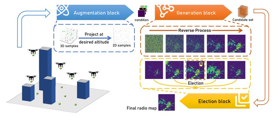
Figure 1: RadioLAM–a large AI model for fine-grained 3D radio map estimation.

In order to deal with the ultra-sparse sampling challenge, we leverage the advanced Artificial Intelligence (AI) technique of Large AI Model (LAM) and propose RadioLAM for 3D radio map estimation:

• Creative power: Unlike traditional discriminative AI, LAM employs generative AI techniques and exhibits “out-of-the-box thinking” abilities to produce diverse outputs from limited inputs. For the problem of 3D radio map estimation, we exploit this property to generate a candidate set of diverse fine-grained radio maps for the target 2D area, from ultra-sparse sampling. Although most of the maps in the candidate set may be inaccurate, we expect that the best map in the set is accurate, enabled by the creative power of LAM.

• Generalization capability: Unlike traditional small-scale AI model, LAM has a strong generalization capability of producing high-quality outputs even when presented with inputs that deviate from the training distribution. For the problem of 3D radio map estimation, we leverage this property to make high-quality radio map estimations for unseen 3D environments not represented in the training dataset, and also to enhance the performance for 3D environments similar to the training dataset.

Specifically, as shown in Fig. 1, RadioLAM consists of three key blocks: an augmentation block, a generation block, and an election block. In the augmentation block, RadioLAM applies the principle of radio propagation to spatially project the radio samples collected at different altitudes (heights) onto the target 2D plane (at the desired altitude), incorporating environmental priors such as terrain features and building layouts to enhance projection accuracy. In the generation block, RadioLAM employs an LAM to generate a candidate set of fine-grained radio maps for the target 2D plane, based on the radio projections which are the outputs of the augmentation block. RadioLAM uses a Mixture of Experts (MoE) architecture for the design of LAM to efficiently enhance the generative performance of LAM across diverse 3D environments. Because of the ultra-small sampling rate, the majority of the maps in the candidate may be inaccurate, with only a minority being accurate. Then in the election block, RadioLAM selects the best map from the candidate set, by using the radio propagation principle as a guide to identify the map demonstrating the closest adherence to the principle. Besides, in the election block, RadioLAM also leverages a Test-Time Adaptive (TTA) scheme to dynamically adjust the generative noise level of LAM during inference, to maintain an effective balance between output diversity and physical plausibility of LAM.

The main contributions of this paper are summarized as follows:

• We study the fine-grained 3D radio map estimation problem which aims to construct high-resolution radio maps for target 2D areas at desired altitudes (target heights) within a 3D space of interest, using radio samples collected at different heights throughout that 3D region. This problem is challenging because the number of collected radio samples is far fewer than the high-resolution requirement of the radio map to be estimated. We develop RadioLAM – a novel LAM which addresses this challenge by the creative power and the strong generalization capability of LAM. To the best of our knowledge, we are the first to take into account the challenge of ultra-sparse sampling when designing algorithms to solve the 3D radio map estimation problem.

• RadioLAM consists of three key blocks: 1) an augmentation block, which leverages the principle of radio propagation to spatially project the multi-altitude radio samples collected by sensors onto the target 2D area at the desired altitude; 2) a generation block, which employs an LAM under the MoE architecture to generate a candidate set of fine-grained radio maps for the target 2D area, based on the radio projections from the augmentation block; 3) an election block, which uses the radio propagation principle as a guide to find the best map from the diverse candidates generated by the generation block, and utilizes a TTA scheme to dynamically adjust the noise level of LAM during inference. With the three blocks, RadioLAM is able to obtain high-quality solutions for the fine-grained 3D radio map estimation problem from ultra-sparse sampling.

• Extensive simulations based on the open-source 3D radio map dataset SpectrumNet show that RadioLAM is effective for constructing fine-grained radio maps across diverse 3D radio propagation environments at different target altitudes. Specifically, simulations show that for different environments, including rural, suburban, ordinary urban, and dense urban, and for different target altitudes, 1) RadioLAM produces high-quality, fine-grained radio maps from an ultra-small sampling rate of $0.1\%$; 2) radio maps generated by RadioLAM are over $50\%$ better than those generated by state-of-the-art (SOTA) under the $0.1\%$ sampling rate; 3) RadioLAM requires at most one fourth of the sampling rate needed by SOTA to construct radio maps with comparable qualities.

The rest of the paper is organized as follows. In Section II, we describe the system model and introduce the 3D radio map estimation problem. In Section III, we present the key ideas of the design of RadioLAM. In Section IV, we offer the design details of RadioLAM. In Section V, we perform extensive simulations to evaluate RadioLAM. In Section VI, we conclude the paper.

II Problem Description

TABLE I: Summary of key notations.

Symbol	Definition
$\mathcal{A}$	3D area of interest
$k$	number of sensors collecting radio samples at different heights within $\mathcal{A}$
$\mathcal{S}$	set of $k$ sensors that collect radio samples at different heights within $\mathcal{A}$
$X$	length of the discrete $\mathcal{A}$
$Y$	width of the discrete $\mathcal{A}$
$H$	height of the discrete $\mathcal{A}$
$\mathbf{S}_{k}$	an $X\times Y\times H$ matrix, where the element at index $(x,y,h)$ is 0 if there is no sensor located at that grid point; otherwise, it is the RSS value of the sample collected by the sensor
$\mathbf{B}$	layout of buildings and an $X\times Y\times H$ matrix, where the element at index $(x,y,h)$ is $1$ if certain building is located at that grid point; otherwise, it is $0$
$\mathbf{T}$	feature of terrain and an $X\times Y$ matrix, where the element at index $(x,y)$ specifies the local ground altitude at the horizontal position $(x,y)$
$h_{t}$	the desired altitude (target height) of the 2D plane where a high-resolution radio map is required to be estimated from $\mathbf{S}_{k}$, $\mathbf{B}$, and $\mathbf{T}$

Let $\mathcal{A}\subset\mathbb{R}^{3}$ represent a 3D area of interest. Within this space, consider a set of sensors $\mathcal{S}=\{1,2,\cdots,k\}$ (the number of sensors is $k$) where each sensor $s\in\mathcal{S}$ is located at a unique 3D coordinate $a_{s}\in\mathcal{A}$. Each sensor $s$ collects a radio sample that measures the RSS $r_{s}(f)$ in a frequency band $f\in\mathcal{F}$ at the location $a_{s}$. These radio samples $r_{s}(f)$ ($s\in\mathcal{S}$ and $f\in\mathcal{F}$) are reported to a fusion center (e.g., a base station or a cloud server). To facilitate analysis, in this paper, we restrict our consideration to a single frequency $f$, considering only spatial samples with RSS $r_{s}$ for each $s\in\{1,2,\cdots,k\}$ at the location $a_{s}\in\mathcal{A}$.

We discretize the continuous spatial area $\mathcal{A}$ into a structured grid of dimension $X\times Y\times H$, where each sensor location $a_{s}$ maps to a unique grid index $(x_{s},y_{s},h_{s})$. Here $x_{s}\in\{0,1,\cdots,X-1\}$ and $y_{s}\in\{0,1,\cdots,Y-1\}$ represent horizontal coordinates, while $h_{s}\in\{0,1,\cdots,H-1\}$ denotes the vertical altitude (height) index. Define $\mathbf{S}_{k}$ as an $X\times Y\times H$ matrix, where its element at index $(x,y,h)$, i.e., $\mathbf{S}_{k}(x,y,h)$, is 0 if there is no sensor located at that grid point; otherwise, it is the RSS value of the sample collected by the sensor located at $(x,y,h)$.

To establish realistic environmental modeling, we take into account environmental obstacles, specifically buildings and terrain characteristics. The layout of buildings is represented by an $X\times Y\times H$ binary matrix $\mathbf{B}$, where its element at index $(x,y,h)$, i.e., $\mathbf{B}(x,y,h)$, is $1$ if certain building is located at that grid point; otherwise, it is $0$. The characteristic of terrain is represented by an $X\times Y$ elevation matrix $\mathbf{T}$, where its element at index $(x,y)$, i.e., $\mathbf{T}(x,y)$, specifies the local ground altitude at the horizontal position $(x,y)$. Both buildings and terrain span the entire 3D area $\mathcal{A}$, potentially occupying multiple adjacent grid points. We consider the occupied grid points to have no RSS; however, they do affect RSS in surrounding areas by reflecting radio waves back into the environment and by blocking or attenuating radio waves passing through them.

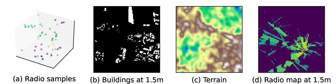
Figure 2: An example of the fine-grained 3D radio map estimation problem, with an objective of using (a), (b), and (c) to produce (d).

Given a desired altitude (target height) $h_{t}\in\{0,1,\cdots,H-1\}$, the problem of fine-grained 3D radio map estimation requires the fusion center to use $\mathbf{S}_{k}$, $\mathbf{B}$, and $\mathbf{T}$ to infer (estimate) the RSS values at grid points $(x,y,h_{t})$ for all $x\in\{0,1,\cdots,X-1\}$ and all $y\in\{0,1,\cdots,Y-1\}$. Fig 2 shows an example of the fine-grained 3D radio map estimation problem. Fig 2a describes radio samples collected within the 3D area $\mathcal{A}$. Fig 2b shows layout of buildings for the target 2D plane at height $1.5$m. Fig 2c illustrates terrain features. Fig 2d gives an estimated fine-grained radio map for the target 2D plane at height $1.5$m. In this example, the problem of 3D radio map estimation requires to use Fig 2a, Fig 2b, and Fig 2c to predict Fig 2d.

III RadioLAM: Basic Ideas

The problem of fine-grained 3D radio map estimation is very challenging due to the extreme sparsity of collected radio samples relative to the high-resolution requirement for the radio map to be estimated. To overcome this challenge and solve the problem, we propose RadioLAM -— an algorithm that leverages the creative power and the strong generalization capability of LAM to estimate radio maps from ultra-sparse sampling for a 3D area of interest.

As shown in Fig. 3, RadioLAM consists of three key blocks: an augmentation block, a generation block, and an election block. In the following, we briefly describe functions of these three blocks, respectively.

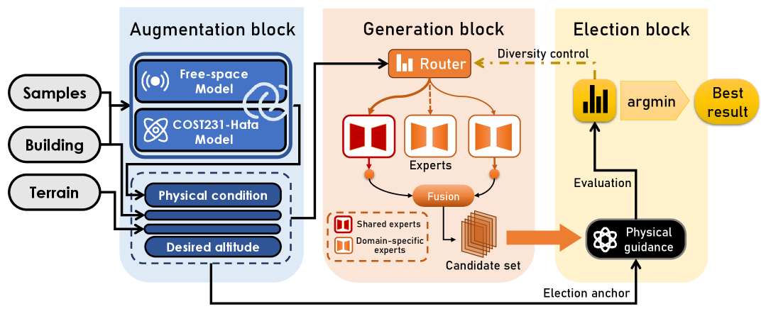
Figure 3: RadioLAM – an architecture overview.

Block 1: Augmentation block The 3D radio map estimation is challenging due to the fact that the number of radio samples, i.e., $k$, is extremely small in practice, resulted from the high costs of sensors capable of collecting radio samples and the large-scale spatial coverage of the 3D area $\mathcal{A}$. Furthermore, the number of radio samples collected at the target height $h_{t}$ can be significantly smaller than $k$ or possibly $0$. Therefore, it is impossible to estimate the radio map for the target 2D plane at height $h_{t}$ only from the coplanar radio samples. To improve the qualities of fine-grained radio maps generated in the subsequent generation block for the target 2D plane, in the augmentation block, we leverage the principle of radio propagation to intelligently project the set of $k$ multi-altitude radio samples onto the target 2D plane at height $h_{t}$. This spatial transformation incorporates environmental parameters, including building layouts and terrain features. The output of this process produces enhanced RSS estimates across the target 2D plane, effectively creating a denser set of virtual RSS measurements than could be obtained through direct sampling at the target height $h_{t}$ alone. These projected RSS values then serve as the inputs for the subsequent generation block.

Block 2: Generation block In this block, we use a diffusion-based LAM to produce a candidate set of diverse fine-grained radio maps for the target 2D plane, from the projected RSS values at different locations in that plane. LAM has an “out-of-the-box thinking” ability, enabling diverse solution generation from sparse inputs. While many candidates may be inaccurate, we expect that the solution space typically contains a few accurate solutions. Moreover, LAM has a strong generalization capability, enabling robust performance even with input distributions that deviate from the training scenarios. For the problem of fine-grained 3D radio map estimation, we use an LAM to generate multiple fine-grained radio maps (64 in simulations) for the target 2D plane from only sparse (less than $0.1\%$ in simulations) radio samples collected at different heights across the 3D area $\mathcal{A}$. Furthermore, we leverage an MoE architecture for the design of the LAM, with each expert in the MoE being a radio map generator specializing in distinct propagation environments (rural, suburban, ordinary urban, and dense urban in simulations). With the MoE architecture, the performance of LAM for generating high-quality radio maps for different kinds of radio propagation environments can be significantly improved.

Block 3: Election block While the generation block demonstrates strong creative capabilities, a large proportion of its generated radio map candidates may be of low quality. It is necessary to design an election block following the generation block to identify the best map in the candidate set. Specifically, in this block, we evaluate and select the most physically plausible solution from the map candidates, by utilizing the radio propagation principle as a guide to identify the map that most closely adheres to the principle in the candidate set. Moreover, in this block, we implement a TTA scheme to dynamically adjust the noise level of LAM during inference. The objective is to maintain an effective balance between the output diversity and the physical plausibility of LAM, enhancing the robustness of RadioLAM to novel input distributions during inference.

With the above three key blocks, RadioLAM is able to efficiently solve the 3D radio map estimation problem when the sampling rate is extremely low. In the following section, we describe the details of the three blocks of RadioLAM.

IV RadioLAM: Design Details

RadioLAM comprises three key blocks: an augmentation block, a generation block, and an election block. In this section, we describe the design details of each block.

IV-A Augmentation Block

The problem of 3D fine-grained radio map estimation aims to construct a high-resolution radio map for a target 2D plane at a desired altitude $h_{t}$, using radio samples collected within the 3D area of interest $\mathcal{A}$. Since radio samples can be collected at altitudes different from $h_{t}$, it is impossible to construct a radio map for the target 2D plane only using samples collected at altitude $h_{t}$. To address this challenge, the augmentation block projects the radio samples collected at altitudes different from $h_{t}$ onto the target 2D plane, i.e., predicts the RSS value located at $(x_{s},y_{s},h_{t})$ from the sample $s$ collected at the location $(x_{s},y_{s},h_{s})$ for each $s\in\mathcal{S}$ with $h_{s}\neq h_{t}$. This projection significantly increases the number of known or estimated RSS values on the target plane compared to using only samples collected at altitude $h_{t}$. The augmented dataset thereby enables the subsequent generation block to construct high-quality radio maps for the target plane.

For each $s\in\mathcal{S}$ with $h_{s}\neq h_{t}$, to predict the RSS value located at $(x_{s},y_{s},h_{t})$ from that located at $(x_{s},y_{s},h_{s})$, we design an algorithm that combines the free-space propagation model [27] and the Hata propagation model [28].

Free-space Propagation Model From Friis’ free-space propagation formula [27], we have

$$P_{r}(d)=P_{t}\frac{G_{t}G_{r}\lambda^{2}}{(4\pi)^{2}d^{n}L},$$ (1)

where $P_{t}$ is the power fed into the transmitting antenna, $P_{r}$ is the power available at the output terminal of the receiving antenna, $G_{r}$ is the effective area of the receiving antenna, $G_{t}$ is the effective area of the transmitting antenna, $d$ is the distance between antennas, $\lambda$ is the wavelength, $L$ is system loss, and $n$ is path loss exponent.

Consider $\mathcal{T}=\{T_{1},T_{2},\cdots,T_{N}\}$ as the set of transmitters, and each transmitter $\tau\in\mathcal{T}$ is located at $(x_{\tau},y_{\tau},h_{\tau})$. From the Frii’s free-space propagation formula, the received power of the point $p$ located at $(x_{p},y_{p},h_{p})$ can be calculated as:

$$P_{\text{free}}(p)= \sum_{\tau\in\mathcal{T}}\biggl[K_{\tau}\cdot\left((x_{p}-x_{\tau})^{2}\right.$$ (2)

$$\left.+(y_{p}-y_{\tau})^{2}+(h_{p}-h_{\tau})^{2}\right)^{-\frac{n}{2}}\biggr].$$

where

$$K_{\tau}=\frac{P_{\tau}G_{\tau}G_{r}\lambda^{2}}{(4\pi)^{2}L}.$$ (3)

To employ the equation (2) to calculate RSS values, we need to know the location of each transmitter $\tau$ and $K_{\tau}$. We note that locations of transmitters are not the input to our problem. In the augmentation, (i) we use the interpolation-based method RBF [12] to estimate locations of transmitters from collected radio samples; and (ii) use the Levenberg-Marquardt algorithm [29] to estimate $K_{\tau}$.

The RSS value located at $(x_{s},y_{s},h_{t})$ can be accurately predicted by the free-space propagation model when an unobstructed line-of-sight (LOS) path exists between $(x_{s},y_{s},h_{t})$ and locations of transmitters. However, in environments with obstructions such as buildings or terrain that block radio wave propagation, the free-space model yields inaccurate predictions. For non-line-of-sight (NLOS) conditions, an alternative propagation model must be employed to predict RSS values.

Hata Propagation Model We leverage the COST231-Hata model for RSS prediction in NLOS setting. Specifically, we can use Hata model to predict the RSS value located at $(x_{s},y_{s},h_{t})$ from the RSS value of the radio sample collected at $(x_{s},y_{s},h_{s})$. According to the Hata model, we have

$$PL=\beta-a(h),$$ (4)

where $PL$ is path loss, and the value of $\beta$ depends on many parameters including the frequency band, information of transmitters, and distance from transmitters. However, the value of $\beta$ remains same for the location $(x_{s},y_{s},h_{t})$ and $(x_{s},y_{s},h_{s})$. We only need to calculate $a(h_{t})$ and $a(h_{s})$ in order to predict the RSS at $(x_{s},y_{s},h_{t})$ from that at $(x_{s},y_{s},h_{s})$:

$$P_{\text{Hata}}(p)=P_{\text{Hata}}(\hat{p})+a(h_{\hat{p}})-a(h_{p}),$$ (5)

where the points $p$ and $\hat{p}$ share the same horizontal position, i.e., $x_{p}=x_{\hat{p}}$ and $y_{p}=y_{\hat{p}}$. $a(\cdot)$ is a correction factor for mobile antenna height. The specific function of $a(\cdot)$ can be found in [28].

When there does not exist a LOS path between the location $(x_{s},y_{s},h_{t})$ and locations of transmitters, the corresponding RSS value predicted by Hata will be much more accurate than that predicted by the free-space propagation model. However, when there exists a LOS path between $(x_{s},y_{s},h_{t})$ and locations of transmitters, the corresponding RSS value predicted by the free-space propagation model will be much more accurate than that predicted by Hata. As a result, ideally, we would like to use the free-space propagation model for RSS predictions of LOS locations and the Hata model for RSS predictions of NLOS locations (Fig. 4 gives an example of LOS locations and NLOS locations). However, figuring out LOS and NLOS locations from building layouts, terrain features, and radio samples (inputs of our problem) is quite challenging. In the augmentation block, instead of trying to find LOS and NLOS locations, we combine the two propagation models and get the following:

$$P_{\text{aug}}(p)=(1-w)\cdot P_{\text{free}}(p)+w\cdot P_{\text{Hata}}(p),$$ (6)

where $w\in(0,1)$ is a weight factor. From Fig. 4, we observe that LOS locations are typically located at high altitudes, while NLOS locations are typically located at low altitudes. Motivated by this observation, we use the following definition for $w$:

$$w=2^{-\frac{h_{p}}{U}},$$ (7)

where $U$ is a positive hyperparameter. For $p$ located at a high altitude, $w$ will be small and hence the free-space propagation model will play a more important role in RSS prediction compared to the Hata model; while for $p$ located at a low altitude, $w$ will be large and hence the Hata model will play a more important role in RSS prediction compared to the free-space propagation model.

Figure 4: An illustration of LOS and NLOS locations.

Moreover, it is intuitive that (6) yields higher prediction accuracy for RSS at $(x_{s},y_{s},h_{t})$, when both $(x_{s},y_{s},h_{t})$ and $(x_{s},y_{s},h_{s})$ share the same propagation condition (either both LOS or both NLOS locations), compared to cases where their propagation conditions differ. For example, in Fig. 4, we prefer predicting $D$ from $G$ rather than from $A$; similarly, we prefer predicting $E$ from $B$ rather than from $H$. To optimize the augmentation process, motivated by the above intuition, we add a filtering strategy: considering that the RSS value which is extremely small is more likely to be located at the NLOS region, given a small predefined threshold $\theta$, we will not use the radio sample $s$ for prediction if its RSS value $r_{s}<\theta$, and even when we use $s$ for prediction and obtain a predicted RSS $\hat{r}_{s}$, we will drop $\hat{r}_{s}$ if $\hat{r}_{s}<\theta$.

IV-B Generation Block

The objective of this block is to generate a diverse set of fine-grained radio map candidates for the target 2D plane at altitude $h_{t}$. We design an LAM under a diffusion-based MoE architecture to achieve this goal.

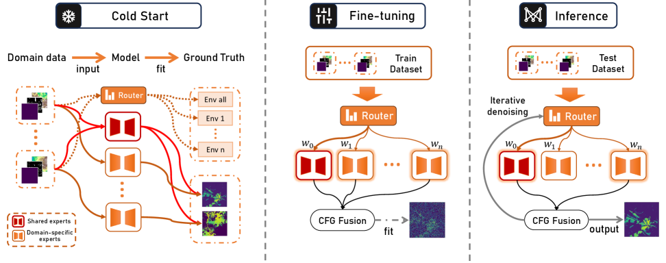
Figure 5: The generation block employs an MoE-based LAM to generate diverse radio map candidates.

We note that in practice, radio propagation characteristics vary significantly across different environments. For example, as shown later in Fig. 6 and Fig. 7 of the evaluation section, urban and rural environments exhibit different radio map patterns. To enhance the generation ability of this block for varying or even unseen propagation characteristics, we use an MoE architecture for the design of LAM. The LAM itself has a strong generalization capability of generating high-quality radio maps for diverse environments. In addition, the MoE architecture incorporates domain-specific experts, each optimized for a particular environmental condition. Compared to using only a monolithic model for generation, the MoE-based model enables better radio map generation for different environments.

Specifically, inspired by the DeepSeekMoE [30] architecture, our diffusion-based LAM consists of a shared expert (generator) handling fundamental propagation patterns, multiple domain-specific experts (generators) specializing in distinct environmental conditions, and a router dynamically selecting appropriate experts by generating different weights for them, as shown in Fig. 5. The training of this LAM employs a two-phase approach: a cold start phase and a fine-tuning phase:

• Cold start of training: The objective of this phase is to utilize available dataset to train the shared expert, domain-specific experts, and router, separately. The shared expert has a UNet structure and will be trained by the complete radio map dataset, complete building layout dataset, and complete terrain feature dataset. Each domain-specific expert also has a UNet structure but will be trained only by the radio map data, building layout data, and terrain feature data corresponding to the specialized domain (environment). For all the experts, we employ the training method of Denoising Diffusion Probabilistic Model (DDPM) [31]. The router has a ResNet18 structure and will be trained by the complete building layout dataset and complete terrain feature dataset, both of which are pre-labeled.

• Fine-tuning of training: The objective of this phase is to update the parameters of the shared expert, domain-specific experts, and router simultaneously by training on the complete dataset. Let all experts and router be activated in this phase. For the complete dataset including radio maps, building layouts, and terrain features, in each instance, the router will first generate different weights for different experts. Then, each expert will generate radio maps based on the radio samples, building layout, and terrain feature. Finally, the generated radio maps from all experts will be fused using the Classifier-Free Guidance (CFG) [32] as the fusion method based on the weights from the router.

During inference, the MoE-based LAM leverages a Denoising Diffusion Implicit Model (DDIM) [33] procedure to generate radio map candidates. DDIM is an iterative procedure. In each iteration, it consists of a forward process (diffusion process) which adds noise to radio maps and a reverse process (inverse diffusion process) which generates radio maps through denoising. In each iteration, the radio samples, building layout, and terrain feature will be the inputs to LAM. For LAM, first, the router will generate different weights for different experts based on the building layout and terrain feature. Then, only the shared expert and the domain-specific expert with the largest weight will be activated to generate radio maps based on all inputs. Next, radio maps generated by the activated experts will be fused using CFG. Compared to DDPM, DDIM significantly reduces the inference time while preserving the high quality of the generated results. Besides, DDIM can be seamlessly applied after DDPM-based model training, allowing for a straightforward conversion of a DDPM model to a DDIM model without the need for retraining. At the end of the iterative DDIM-based inference, LAM will produce a candidate set of diverse fine-grained radio maps.

IV-C Election block

The objective of this block is to identify the best map in the diverse set of fine-grained radio map candidates generated by the generation block. We employ a radio propagation model (consistent with our augmentation block) as a guide to identify the candidate that demonstrates the highest conformance to it and consider such a candidate as the best map. Moreover, we incorporate a TTA-based scheme in this block, to dynamically adjust the noise level of LAM, ensuring both the generation diversity and physical plausibility of LAM.

Considering that the true radio map (ground truth) is unknown during inference, it is impossible to directly find the best map from the candidate set based on a comparison to the true map. Although the RSS value of each location in the target 2D plane at altitude $h_{t}$ (i.e., each location in the trure map) is unknown, at the end of the augmentation block, we know RSS values of several locations in the 2D plane at altitude $h_{t}$. These RSS values either come from radio samples collected at altitude $h_{t}$, or are predicted (projected) by radio samples collected at the same horizontal positions but at different altitudes using the radio propagation model (6). Intuitively, we can compare the radio map candidates with these RSS values to identify the best one.

Specifically, suppose $\bar{r}_{s}$ is the RSS value of the location $(x_{s},y_{s})$ in the generated radio map. Suppose $\hat{r}_{s}$ is the RSS value predicted from the radio sample $s\in\mathcal{S}$ with $h_{s}\neq h_{t}$ in the augmentation block (let $\hat{r}_{s}=r_{s}$ if $h_{s}=h_{t}$, and let $\hat{r}_{s}=\bar{r}_{s}$ if we do not project $s$ onto the target 2D plane). For each map in the candidate set, we calculate the following distance metric:

$$D_{\text{ele}}~=~\sum_{s\in\mathcal{S}}(\bar{r}_{s}-\hat{r}_{s})^{2}.$$ (8)

We consider the radio map that minimizes $D_{\text{ele}}$ among all the maps in the candidate set as the best map.

Note that RadioLAM addresses the ultra-sparse sampling challenge of 3D radio map estimation using the creative power of LAM, by generating a diverse set of radio map candidates from ultra-small number of radio samples. At the end of this election block, we design a control algorithm to maintain appropriate diversity of LAM, by adjusting LAM’s noise level based on the variance of qualities of the radio map candidates.

Considering that for each radio map candidate, we can quantify its quality by calculating the distance metric (8). Then, we quantify the diversity of radio map candidates by calculating the variance of corresponding distance metrics. Let Var be such a variance. We optimize the diversity of LAM by adjusting the zero-mean noise which we inject to the CFG weights during the CFG-based fusion of LAM:

$$\sigma_{t+1}=\left\{\begin{array}[]{ll}\min(\sigma_{t}+\Delta\sigma,\sigma_{m}),&\text{Var}<V\\ \sigma_{t}/2,&\text{Var}\geq V\end{array}\right.$$ (9)

where $\sigma_{t}$ is the variance of the zero-mean noise at the current timestep $t$, $\sigma_{t+1}$ is the variance of the zero-mean noise at the next timestep $t+1$, $\Delta\sigma$ is a hyperparameter of increment step, $V$ is a hyperparameter of variance threshold, and $\sigma_{m}$ is a hyperparameter of noise threshold. With this mechanism, the noise will increase if the current output diversity of LAM is relatively low; otherwise, the noise will reduce. As a result, the output diversity of LAM is expected to remain at an appropriate level.

V Evaluation

In this section, we evaluate RadioLAM. We first use a case study to evaluate its performance and demonstrate its capability of constructing fine-grained radio maps for target 2D planes across a 3D area of interest from ultra-sparse sampling. Then we use extensive simulations to compare it against various baseline algorithms, by estimating radio maps for different 2D planes at varying heights across diverse kinds of 3D environments. Next, we conduct ablation studies to analyze the individual contributions of the augmentation block, the generation block, and the election block to its overall performance. Finally, we evaluate its performance under varying model sizes (i.e., different numbers of model parameters).

V-A Simulation Settings

We use the open-source dataset SpectrumNet [26] for the evaluation. SpectrumNet consists of radio maps in 5 different frequency bands: 150 MHz, 1.5 GHz, 1.7 GHz, 3.5 GHz and 22 GHz. It includes 11 different kinds of geographical environment: dense urban, ordinary urban, suburban, rural, mountainous, forest, desert, grassland, island, ocean, and lake. It takes into account the joint impact of terrain features and building layouts on radio propagation. It uses OpenStreetMap [34] to obtain real-world building layouts and terrain features of $15300$ different areas, each of which has a size of $1.28$km $\times$ $1.28$km in the horizontal plane, with a spacial resolution of $10$m, resulting in radio maps of resolution $128\times 128$ (i.e., $X=Y=128$). There may exist multiple transmitters in each area. It utilizes Matlab to obtain radio maps at $3$ different heights for each area: $1.5$m, $30$m, and $200$m (i.e., $H=3$).

For our evaluation, we focus on the frequency band of 3.5GHz and geographical environment of dense urban, ordinary urban, suburban, and rural. We use 6327 maps for training and 1590 maps for inference (evaluation). We consider the number of samples collected by sensors within one 3D area, i.e., $k$, to be $50$, unless otherwise specified. As a result, we use an extremely small sampling rate of $0.1\%$ for evaluation. For each $128\times 128\times 3$ 3D area, the specific locations of $k$ radio samples are randomly generated.

We implement RadioLAM on two NVIDIA RTX 4090 GPUs. The size (number of parameters) of RadioLAM is $0.6$ billion, unless otherwise specified. The training procedure is sped up by the DeepSpeed ZeRO-2 [35] optimization framework. Deep learning codes are built using PyTorch. We set the number of DDPM inference steps as 1000, and the number of DDIM inference steps as 10. There are 64 radio map candidates generated by the generation block for each target 2D plane in each problem instance.

To evaluate RadioLAM, we compare it with the following two interpolation-based baseline algorithms:

• 3D-RBF [12]: It directly extends the algorithm RBF from 2D radio map estimation to 3D radio map estimation. By creating a network of basis functions around the known data points, it uses a linear combination of these basis functions to approximate the values of unknown points.

• 3D-kriging [14]: It directly extends the algorithm kriging from 2D radio map estimation to 3D radio map estimation. It uses a semi-variogram function to describe the spatial autocorrelation and estimates the values of unknown points by weighted average of the observed data of known points.

In addition, we compare RadioLAM with the following two existing deep learning-based approaches which solve the 3D radio map estimation problem:

• 3D-UNet [24]: It uses a UNet model for 3D radio map estimation. UNet is a convolutional neural network (CNN) featuring a symmetric encoder-decoder structure. The encoder progressively compresses spatial information through downsampling, while the decoder reconstructs high-quality features via upsampling operations.

• 3D-DCRGAN [22]: Adapted from the GAN framework proposed in [22] for 3D radio map estimation, this baseline approach removes the original algorithm’s dependence on transmitters’ information to maintain consistency with our problem formulation (which does not require the prior knowledge of transmitters’ information).

Note that our 3D radio map estimation problem aims to estimate the radio map for a target 2D plane at height $h_{t}$ from radio samples in $\mathcal{S}$. Each radio sample $s\in\mathcal{S}$ gives the RSS value located at $(x_{s},y_{s},h_{s})$ where the height $h_{s}$ can be different from the target height $h_{t}$. For evaluation, we further compare RadioLAM with two existing deep learning-based methods, i.e., Autoencoder [36] and RadioUNet [15], both of which solve the 2D radio map estimation problem from the RSS values at locations $(x_{s},y_{s},h_{t})$ for all $s\in\mathcal{S}$. Considering that $\{(x_{s},y_{s},h_{s}),s\in\mathcal{S}\}$ rather than $\{(x_{s},y_{s},h_{t}),s\in\mathcal{S}\}$ are inputs to our problem, the baseline methods Autoencoder and RadioUNet only represent idealized performance benchmarks rather than practical solutions for our problem. If the practical model RadioLAM outperforms the two idealized baselines, it will be convincing that RadioLAM is effective for 3D radio map estimation.

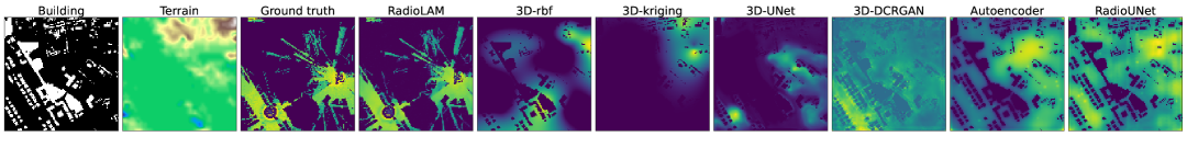
(a)

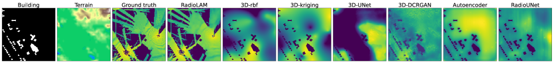
(b)

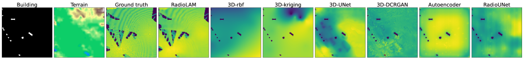
(c)

Figure 6: Fine-grained radio maps constructed by different algorithms in the case study (ordinary urban environment).

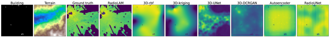
(a)

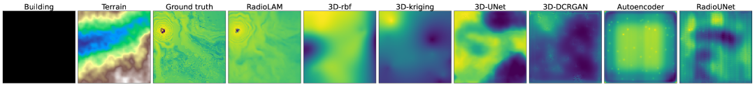
(b)

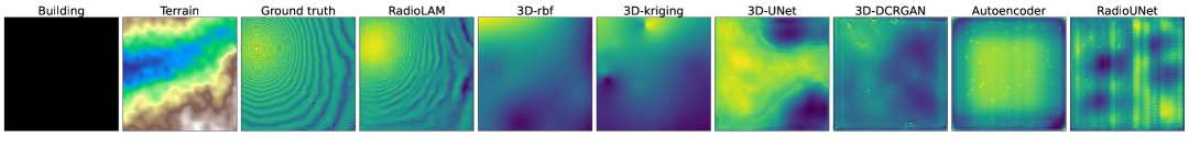
(c)

Figure 7: Fine-grained radio maps constructed by different algorithms in the case study (rural environment).

To quantify the performance of algorithms, Mean Absolute Error (MAE), Mean Square Error (MSE), and Peak Signal to Noise Ratio (PSNR) are used:

• MAE: It measures the average absolute difference between predicted and true values.

  $$\text{MAE}=\frac{1}{X\times Y}\sum^{X-1}_{x=0}\sum^{T-1}_{y=0}|I(x,y)-\hat{I}(x,y)|,$$ (10)

  where $I(x,y)$ is the true RSS value at the location $(x,y,h_{t})$ and $\hat{I}(x,y)$ is the predicted RSS value at that location.

• MSE: It is the average of the squared difference between predicted and true values.

  $$\text{MSE}=\frac{1}{X\times Y}\sum^{X-1}_{x=0}\sum^{T-1}_{y=0}[I(x,y)-\hat{I}(x,y)]^{2},$$ (11)

• PSNR [37]: It estimates the ratio between the maximum RSS and the square root of MSE, and is usually expressed as a logarithmic quantity using the decibel scale.

  $$\text{PSNR}=20\cdot\log_{10}\left(\frac{\text{MAX}_{I}}{\sqrt{\text{MSE}}}\right),$$ (12)

  where $\text{MAX}_{I}$ is the maximum RSS value of a point on the radio map.

A small MAE, a small MSE, or a large PSNR implies that the constructed radio map is of high quality.

V-B Simulation Results

Case Study In the case study, we evaluate the performance of different algorithms across two distinct environments: an ordinary urban instance and a rural instance. Fig. 6 shows the building layouts, terrain features, and fine-grained radio maps estimated by different algorithms for an ordinary urban instance (Fig. LABEL:E8-1.5 shows the radio maps estimated at height $1.5$m, Fig. LABEL:E8-30 shows the radio maps estimated at height $30$m, and Fig. LABEL:E8-200 shows the radio maps estimated at height $200$m). Similarly, Fig. 7 shows the building layouts, terrain features, and fine-grained radio maps estimated by different algorithms for a rural instance (Fig. LABEL:E7-1.5 shows the radio maps estimated at height $1.5$m, Fig. LABEL:E7-30 shows the radio maps estimated at height $30$m, and Fig. LABEL:E7-200 shows the radio maps estimated at height $200$m).

From the two figures, it is clear that the fine-grained radio maps constructed by RadioLAM are quite close to the ground truth (true radio maps), for both environments at all $3$ different altitudes (heights). In sharp contrast, the radio maps constructed by any of the 6 baseline algorithms significantly deviate from the true radio maps and hence are extremely inaccurate.

TABLE II: Simulation results for the ordinary urban environment in the case study.

Performance metric	MAE			MSE			PSNR
Target height $h_{t}$	1.5m	30m	200m	1.5m	30m	200m	1.5m	30m	200m
3D-RBF	0.1301	0.1790	0.1093	0.0398	0.0508	0.0232	13.998	12.938	16.340
3D-kriging	0.1289	0.1757	0.0686	0.0433	0.0476	0.0138	13.625	13.215	18.579
Autoencoder	0.1348	0.1399	0.0871	0.0287	0.0288	0.0111	15.413	15.396	19.513
RadioUNet	0.1381	0.1562	0.1019	0.0265	0.0288	0.0145	15.755	15.393	18.365
3D-UNet	0.1014	0.1572	0.0820	0.0286	0.0465	0.0133	15.423	13.317	18.741
3D-DCRGAN	0.1054	0.2169	0.2964	0.0236	0.0652	0.0960	16.257	11.856	10.172
RadioLAM	0.0169	0.0252	0.0182	0.0025	0.0032	0.0013	25.937	24.849	28.796

Table II presents the MAE, MSE, and PSNR results achieved by different algorithms for the ordinary urban environment. The results indicate that in general, RadioLAM achieves over $70\%$ reduction in MAE, over $85\%$ reduction in MSE, and over $45\%$ improvement in PSNR compared to all baseline algorithms. Interestingly, while these quantitative metrics, e.g., MAE, show that RadioLAM outperforms baseline algorithms by $70\%$, visual analysis in Fig. 6 reveals a more substantial qualitative difference. In Fig. 6, the radio map constructed by RadioLAM is very close to the true map, but those constructed by baseline algorithms significantly deviate from the true map. This suggests potential limitations in using conventional performance metrics MAE, MSE, and PSNR for quality evaluation of radio maps. We leave it as an important future direction to design better performance metrics for quantifying the quality of estimated radio maps.

More Simulations Then we perform more simulations to evaluate RadioLAM. Table III presents the simulation results comparing RadioLAM with $6$ baseline algorithms for radio map estimation of $4$ different kinds of 3D environments at $3$ different target heights. Given one specific kind of 3D environment, we simulate 100 instances and for each instance, we use RadioLAM as well as baseline approaches to construct radio maps for 2D planes at the target heights $h_{t}=1.5$m, $h_{t}=30$m, and $h_{t}=200$m, respectively. The reported metrics (MAE, MSE, and PSNR) in Table III represent the average values obtained from 100 instances.

TABLE III: Simulation results for different kinds of environments where 100 instances are simulated for each environment.

MAE
3D environment	Suburban			Dense urban			Rural			Ordinary urban
Target height $h_{t}$	1.5m	30m	200m	1.5m	30m	200m	1.5m	30m	200m	1.5m	30m	200m
3D-RBF	0.1782	0.1155	0.0364	0.1252	0.1501	0.0538	0.1906	0.1319	0.0416	0.1533	0.1442	0.0602
3D-kriging	0.1706	0.0773	0.0255	0.1055	0.1283	0.0407	0.1788	0.0837	0.0296	0.1432	0.1203	0.0453
Autoencoder	0.1771	0.1564	0.1405	0.1286	0.1451	0.1192	0.1904	0.1716	0.1632	0.1684	0.1628	0.1359
RadioUNet	0.1854	0.1315	0.1067	0.1443	0.1865	0.1629	0.1951	0.1240	0.0936	0.1743	0.1619	0.1089
3D-UNet	0.1916	0.1686	0.0477	0.0925	0.2609	0.0956	0.1797	0.1726	0.0494	0.1352	0.2097	0.0855
3D-DCRGAN	0.2438	0.1982	0.0521	0.1109	0.1760	0.0572	0.2036	0.1509	0.0421	0.1621	0.1739	0.0687
RadioLAM	0.0792	0.0497	0.0165	0.0512	0.0807	0.0249	0.0848	0.0541	0.0190	0.0555	0.0684	0.0311
MSE
3D environment	Suburban			Dense urban			Rural			Ordinary urban
Target height $h_{t}$	1.5m	30m	200m	1.5m	30m	200m	1.5m	30m	200m	1.5m	30m	200m
3D-RBF	0.0557	0.0297	0.0039	0.0379	0.0403	0.0088	0.0619	0.0351	0.0053	0.0497	0.0418	0.0126
3D-kriging	0.0514	0.0188	0.0023	0.0321	0.0346	0.0063	0.0546	0.0208	0.0035	0.0449	0.0340	0.0086
Autoencoder	0.0382	0.0281	0.0221	0.0257	0.0295	0.0172	0.0409	0.0322	0.0286	0.0363	0.0325	0.0222
RadioUNet	0.0427	0.0238	0.0155	0.0258	0.0416	0.0308	0.0514	0.0226	0.0115	0.0397	0.0334	0.0163
3D-UNet	0.0574	0.0484	0.0051	0.0244	0.0953	0.0192	0.0470	0.0505	0.0055	0.0380	0.0701	0.0137
3D-DCRGAN	0.0857	0.0514	0.0045	0.0324	0.0404	0.0071	0.0594	0.0345	0.0038	0.0497	0.0423	0.0096
RadioLAM	0.0224	0.0108	0.0013	0.0153	0.0193	0.0030	0.0249	0.0123	0.0019	0.0165	0.0182	0.0056
PSNR
3D environment	Suburban			Dense urban			Rural			Ordinary urban
Target height $h_{t}$	1.5m	30m	200m	1.5m	30m	200m	1.5m	30m	200m	1.5m	30m	200m
3D-RBF	12.541	15.267	24.119	14.208	13.948	20.559	12.081	14.546	22.741	13.038	13.787	19.000
3D-kriging	12.894	17.259	26.476	14.940	14.615	22.016	12.628	16.826	24.560	13.482	14.683	20.637
Autoencoder	14.178	15.513	16.555	15.903	15.306	17.647	13.887	14.922	15.439	14.400	14.882	16.539
RadioUNet	13.695	16.227	18.103	15.882	13.807	15.108	12.890	16.456	19.408	14.015	14.758	17.875
3D-UNet	12.411	13.153	22.933	16.124	10.209	17.173	13.275	12.964	22.600	14.207	11.543	18.647
3D-DCRGAN	10.672	12.893	23.484	14.899	13.934	21.510	12.262	14.621	24.254	13.038	13.738	20.193
RadioLAM	16.504	19.675	28.994	18.149	17.152	25.237	16.030	19.101	27.243	17.830	17.410	22.546

From the table, we observe that RadioLAM significantly outperforms all baseline algorithms. Specifically,

• As compared to existing 3D radio map estimation algorithms 3D-UNet and 3D-DCRGAN, (1) in the suburban environment, RadioLAM reduces MSE by $60\%$ at height $1.5$m, by $77\%$ at height $30$m, and by $71\%$ at height $200$m; (2) in the dense urban environment, RadioLAM reduces MSE by $37\%$ at height $1.5$m, by $52\%$ at height $30$m, and by $57\%$ at height $200$m; (3) in the rural environment, RadioLAM reduces MSE by $47\%$ at height $1.5$m, by $64\%$ at height $30$m, and by $50\%$ at height $200$m; (4) in the ordinary urban environment, RadioLAM reduces MSE by $56\%$ at height $1.5$m, by $56\%$ at height $30$m, and by $41\%$ at height $200$m.

• As compared to interpolation-based baseline algorithms 3D-RBF and 3D-kriging, (1) in the suburban environment, RadioLAM reduces MSE by $56\%$ at height $1.5$m, by $42\%$ at height $30$m, and by $43\%$ at height $200$m; (2) in the dense urban environment, RadioLAM reduces MSE by $52\%$ at height $1.5$m, by $44\%$ at height $30$m, and by $52\%$ at height $200$m; (3) in the rural environment, RadioLAM reduces MSE by $54\%$ at height $1.5$m, by $40\%$ at height $30$m, and by $31\%$ at height $200$m; (4) in the ordinary urban environment, RadioLAM reduces MSE by $63\%$ at height $1.5$m, by $46\%$ at height $30$m, and by $34\%$ at height $200$m.

• As compared to existing 2D radio map estimation algorithms Autoencoder and RadioUNet, (1) in the suburban environment, RadioLAM reduces MSE by $41\%$ at height $1.5$m, by $54\%$ at height $30$m, and by $91\%$ at height $200$m; (2) in the dense urban environment, RadioLAM reduces MSE by $40\%$ at height $1.5$m, by $34\%$ at height $30$m, and by $82\%$ at height $200$m; (3) in the rural environment, RadioLAM reduces MSE by $39\%$ at height $1.5$m, by $45\%$ at height $30$m, and by $83\%$ at height $200$m; (4) in the ordinary urban environment, RadioLAM reduces MSE by $54\%$ at height $1.5$m, by $44\%$ at height $30$m, and by $65\%$ at height $200$m.

From Table III, we can also observe similar huge reductions in MAE and improvements in PSNR comparing RadioLAM with baseline algorithms.

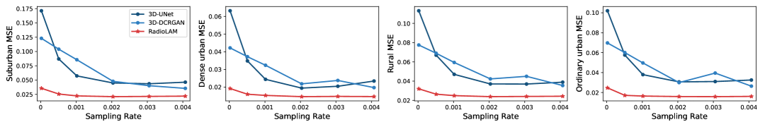
(a)

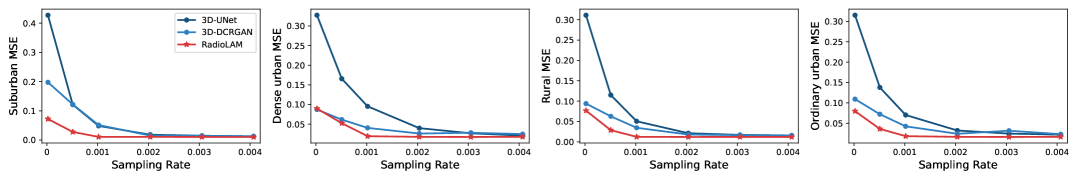
(b)

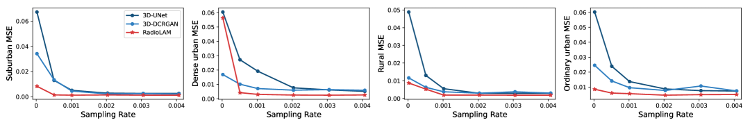
(c)

Figure 8: Simulation results under varying sampling rates.

Fig. 8 presents the MSE results of RadioLAM, 3D-UNet, and 3D-DCRGAN, under varying sampling rates (i.e., $k/(X\cdot Y\cdot H)$). From Fig. 8a (for $h_{t}=1.5$m), we observe that the MSE achieved by RadioLAM is close to $0$ when the sampling rate is only $0.1\%$. However, the MSE achieved by 3D-UNet and 3D-DCRGAN remains much greater than $0$ even when the sampling rate is $0.4\%$. Similar observation can be observed from Fig. 8c for $h_{t}=200$m. From Fig. 8b (for $h_{t}=30$m), the MSE achieved by RadioLAM is close to $0$ when the sampling rate is $0.1\%$, while that achieved by 3D-UNet and 3D-DCRGAN becomes close to $0$ when the sampling rate is $0.2\%$.

Ablation Study RadioLAM consists of three key blocks: an augmentation block, a generation block, and an election block. Now we use ablation studies to evaluate each of them.

TABLE IV: MSE results of simulations that evaluate the augmentation block and election block of RadioLAM.

Suburban
Setting		Target height $h_{t}$
Augmentation block	Election block	1.5m	30m	200m
$\times$	$\times$	0.0322	0.0200	0.0086
$\checkmark$	$\times$	0.0301	0.0140	0.0019
$\times$	$\checkmark$	0.0305	0.0191	0.0079
$\checkmark$	$\checkmark$	0.0224	0.0108	0.0013
Dense urban
Setting		Target height $h_{t}$
Augmentation block	Election block	1.5m	30m	200m
$\times$	$\times$	0.0229	0.0374	0.0153
$\checkmark$	$\times$	0.0207	0.0291	0.0058
$\times$	$\checkmark$	0.0211	0.0366	0.0153
$\checkmark$	$\checkmark$	0.0153	0.0193	0.0030
Rural
Setting		Target height $h_{t}$
Augmentation block	Election block	1.5m	30m	200m
$\times$	$\times$	0.0324	0.0202	0.0077
$\checkmark$	$\times$	0.0305	0.0155	0.0023
$\times$	$\checkmark$	0.0318	0.0173	0.0073
$\checkmark$	$\checkmark$	0.0249	0.0123	0.0019
Ordinary urban
Setting		Target height $h_{t}$
Augmentation block	Election block	1.5m	30m	200m
$\times$	$\times$	0.0245	0.0316	0.0131
$\checkmark$	$\times$	0.0221	0.0288	0.0075
$\times$	$\checkmark$	0.0234	0.0313	0.0114
$\checkmark$	$\checkmark$	0.0165	0.0182	0.0056

TABLE V: MSE results of simulations that evaluate the generation block of RadioLAM.

Suburban
Setting of the	Parameters		Target height $h_{t}$
generation block	Total	Activated	1.5m	30m	200m
Monolithic	$246$M	$246$M	0.0270	0.0139	0.0017
MoE-based	$609$M	$244$M	0.0224	0.0108	0.0013
Dense urban
Setting of the	Parameters		Target height $h_{t}$
generation block	Total	Activated	1.5m	30m	200m
Monolithic	$246$M	$246$M	0.0207	0.0292	0.0056
MoE-based	$609$M	$244$M	0.0153	0.0193	0.0030
Rural
Setting of the	Parameters		Target height $h_{t}$
generation block	Total	Activated	1.5m	30m	200m
Monolithic	$246$M	$246$M	0.0318	0.0155	0.0023
MoE-based	$609$M	$244$M	0.0249	0.0123	0.0019
Ordinary urban
Setting of the	Parameters		Target height $h_{t}$
generation block	Total	Activated	1.5m	30m	200m
Monolithic	$246$M	$246$M	0.0226	0.0277	0.0086
MoE-based	$609$M	$244$M	0.0165	0.0182	0.0056

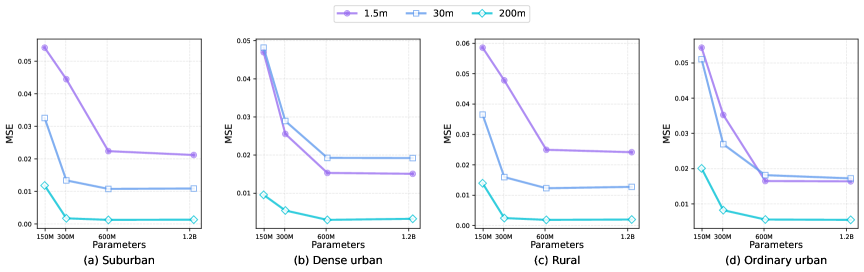
Figure 9: Performance of RadioLAM under varying model sizes (numbers of parameters).

Table IV presents an ablation study evaluating the contribution of the augmentation block and the election block to RadioLAM. Given one specific kind of 3D environment, we simulate 100 instances. This table demonstrates that: (1) removing either the augmentation block or the election block leads to significant performance degradation, confirming both blocks’ critical roles in RadioLAM; (2) the augmentation block exhibits greater impact on the output quality of RadioLAM than the election block, as evidenced by more substantial performance drops when this block is removed.

The generation block is the core of RadioLAM and has a MoE architecture. In this design, each expert in MoE specializes in generating radio maps for a distinct propagation environment. To validate this design, we conduct simulations to compare our MoE-based model with a monolithic baseline using a single diffusion model for all environments. The number of parameters in the monolithic model is $246$ million, consistent with the number of activated parameters in our MoE-based model. Table V shows the simulation results, clearly demonstrating the superior performance of our proposed MoE-based generation over the monolithic generation.

Model Size Analysis Finally, we evaluate the performance of RadioLAM under varying model sizes (numbers of parameters). Fig. 9 demonstrates the MSE results of RadioLAM when the number of parameters is $150$ million, $300$ million, $0.6$ billion, and $1.2$ billion, respectively. From the figure, we observe that when the number of parameters is smaller than $0.6$ billion, the performance improvement of RadioLAM is evident as the number of parameters grows. However, when the number of parameters is greater than $0.6$ billion, the performance improvement of RadioLAM is minor as the number of parameters increases.

VI Conclusion

The problem of fine-grained 3D radio map estimation aims to construct high-resolution radio maps for 2D planes at desired altitudes (target heights) within a 3D area of interest, based on radio samples collected at different locations within that 3D area. This problem is challenging due to the ultra-sparse sampling, i.e., the number of collected samples is significantly smaller than the high resolution of radio maps to be estimated. In this paper, we leverage the creative power and the strong generalization capability of LAM to address the ultra-sparse sampling challenge, and propose RadioLAM for fine-grained 3D radio map estimation. RadioLAM consists of three key blocks: 1) an augmentation block, which leverages the principle of radio propagation to project radio samples collected at varying altitudes onto the target 2D plane at the desired altitude; 2) a generation block, which employs an LAM under an MoE architecture to generate a candidate set of diverse fine-grained radio maps for the target 2D plane, based on projections of radio samples; 3) an election block, which utilizes the radio propagation principle as a guide to find the best map from the candidate set, and uses TTA to dynamically adjust the noise level of LAM during inference.

Extensive simulations based on the open-source 3D radio map dataset SpectrumNet show that for different kinds of radio propagation environments, including rural, suburban, ordinary urban, and dense urban, 1) RadioLAM produces high-quality, fine-grained radio maps from an ultra-small sampling rate of $0.1\%$; 2) fine-grained radio maps generated by RadioLAM are over $50\%$ better than those generated by SOTA under the $0.1\%$ sampling rate; 3) RadioLAM requires at most one fourth of the sampling rate needed by SOTA to construct fine-grained radio maps with comparable qualities. Potential future research includes the design of 3D radio map estimation algorithms with strong theoretical performance guarantees and future radio map prediction from currently collected radio samples.

References

- [1] D. Romero and S.-J. Kim, “Radio map estimation: A data-driven approach to spectrum cartography,” IEEE Signal Processing Magazine, vol. 39, no. 6, pp. 53–72, 2022.
- [2] Y. Peng, Y. Li, Y. Guo, D. Zhang, F. Khan, R. Alturki, and B. Alshawi, “A blockchain-based distributed collaborative sensing and spectrum access approach for consumer electronics,” IEEE Transactions on Consumer Electronics, 2025, early access.
- [3] A. S. Matar and X. Shen, “Joint optimization of user association, power control, and dynamic spectrum sharing for integrated aerial-terrestrial network,” IEEE Journal on Selected Areas in Communications, vol. 43, no. 1, pp. 396–409, 2025.
- [4] J. Huang, L. Lian, D. Wen, Y. Zhou, F. Wang, W. Wang, and Y. Shi, “Dynamic UAV-assisted cooperative edge AI inference,” IEEE Transactions on Wireless Communications, vol. 24, no. 1, pp. 615–628, 2024.
- [5] H. Zhu, U. Demirbaga, G. S. Aujla, L. Shi, and P. Zhang, “Explainable edge AI framework for IoD-assisted aerial surveillance in extreme scenarios,” IEEE Internet of Things Journal, vol. 12, no. 5, pp. 4570–4578, 2025.
- [6] S. Qi, B. Lin, Y. Deng, X. Chen, and Y. Fang, “Minimizing maximum latency of task offloading for multi-UAV-assisted maritime search and rescue,” IEEE Transactions on Vehicular Technology, vol. 73, no. 9, pp. 13 625–13 638, 2024.
- [7] S. Ri, J. Ye, N. Toyama, and N. Ogura, “Drone-based displacement measurement of infrastructures utilizing phase information,” Nature Communications, vol. 15, no. 1, 2024.
- [8] K. Rizk, J.-F. Wagen, and F. Gardiol, “Two-dimensional ray-tracing modeling for propagation prediction in microcellular environments,” IEEE Transactions on Vehicular Technology, vol. 46, no. 2, pp. 508–518, 1997.
- [9] R. Wahl, G. Wölfle, P. Wildbolz, and F. Landstorfer, “Dominant path prediction model for urban scenarios,” in Proc. of IST Mobile and Wireless Communications, Dresden, Germany, June 19-23, 2005.
- [10] J. A. Bazerque and G. B. Giannakis, “Distributed spectrum sensing for cognitive radio networks by exploiting sparsity,” IEEE Transactions on Signal Processing, vol. 58, no. 3, pp. 1847–1862, 2010.
- [11] T. Zugno, M. Drago, M. Giordani, M. Polese, and M. Zorzi, “Toward standardization of millimeter-wave vehicle-to-vehicle networks: Open challenges and performance evaluation,” IEEE Communications Magazine, vol. 58, no. 9, pp. 79–85, 2020.
- [12] C. M. Bishop, Neural Networks for Pattern Recognition. New York, NY, USA: Oxford University Press, Inc., 1995.
- [13] J. A. Bazerque, G. Mateos, and G. B. Giannakis, “Group-lasso on splines for spectrum cartography,” IEEE Transactions on Signal Processing, vol. 59, no. 10, pp. 4648–4663, 2011.
- [14] G. Boccolini, G. Hernández-Peñaloza, and B. Beferull-Lozano, “Wireless sensor network for spectrum cartography based on kriging interpolation,” in Proc. of IEEE PIMRC, Sydney, Australia, September 09-12, 2012.
- [15] R. Levie, Ç. Yapar, G. Kutyniok, and G. Caire, “RadioUNet: Fast radio map estimation with convolutional neural networks,” IEEE Transactions on Wireless Communications, vol. 20, no. 6, pp. 4001–4015, 2021.
- [16] Y. Teganya and D. Romero, “Deep completion autoencoders for radio map estimation,” IEEE Transactions on Wireless Communications, vol. 21, no. 3, pp. 1710–1724, 2022.
- [17] K. He, X. Zhang, S. Ren, and J. Sun, “Deep residual learning for image recognition,” in Proc. of CVPR, Las Vegas, USA, June 27-30, 2016.
- [18] Z. Liu, S. Zhang, Q. Liu, H. Zhang, and L. Song, “WiFi-Diffusion: Achieving fine-grained WiFi radio map estimation with ultra-low sampling rate by diffusion models,” arXiv:2503.12004v2, 2025.
- [19] M. Ayadi, A. Ben Zineb, and S. Tabbane, “A UHF path loss model using learning machine for heterogeneous networks,” IEEE Transactions on Antennas and Propagation, vol. 65, no. 7, pp. 3675–3683, 2017.
- [20] A. Creswell, T. White, V. Dumoulin, K. Arulkumaran, B. Sengupta, and A. A. Bharath, “Generative adversarial networks: An overview,” IEEE Signal Processing Magazine, vol. 35, no. 1, pp. 53–65, 2018.
- [21] X. Li, S. Zhang, H. Li, X. Li, L. Xu, H. Xu, H. Mei, G. Zhu, N. Qi, and M. Xiao, “RadioGAT: A joint model-based and data-driven framework for multi-band radiomap reconstruction via graph attention networks,” IEEE Transactions on Wireless Communications, vol. 23, no. 11, pp. 1–1, 2024.
- [22] T. Hu, Y. Huang, J. Chen, Q. Wu, and Z. Gong, “3D radio map reconstruction based on generative adversarial networks under constrained aircraft trajectories,” IEEE Transactions on Vehicular Technology, vol. 72, no. 6, pp. 8250–8255, 2023.
- [23] L. Zhao, Z. Fei, X. Wang, J. Luo, and Z. Zheng, “3D-RadioDiff: An altitude-conditioned diffusion model for 3D radio map construction,” IEEE Wireless Communications Letters, 2025, early access.
- [24] E. Krijestorac, S. Hanna, and D. Cabric, “Spatial signal strength prediction using 3D maps and deep learning,” in Proc. of IEEE ICC, Virtual Conference, June 14-23, 2021.
- [25] Z. Chen, H. Wang, and D. Guo, “3D radio map estimation based on active measurement trajectory selection,” IEEE Wireless Communications Letters, 2025, early access.
- [26] S. Zhang, S. Jiang, W. Lin, Z. Fang, K. Liu, H. Zhang, and K. Chen, “Generative AI on SpectrumNet: An open benchmark of multiband 3D radio maps,” IEEE Transactions on Cognitive Communications and Networking, vol. 11, no. 2, pp. 886–901, 2025.
- [27] H. Friis, “A note on a simple transmission formula,” Proceedings of the IRE, vol. 34, no. 5, pp. 254–256, 1946.
- [28] P. E. Mogensen, J. Wigard et al., “Cost action 231: Digital mobile radio towards future generation systems, final report,” European Commission, Luxembourg, COST Action 231 EUR 18957, 1999.
- [29] D. W. Marquardt, “An algorithm for least-squares estimation of nonlinear parameters,” Journal of the Society for Industrial and Applied Mathematics, vol. 11, no. 2, pp. 431–441, 1963.
- [30] D. Dai, C. Deng, C. Zhao, R. X. Xu, H. Gao, D. Chen, J. Li, W. Zeng, X. Yu, Y. Wu, Z. Xie, Y. K. Li, P. Huang, F. Luo, C. Ruan, Z. Sui, and W. Liang, “DeepSeekMoE: Towards ultimate expert specialization in mixture-of-experts language models,” 2024. [Online]. Available: https://arxiv.org/abs/2401.06066
- [31] J. Ho, A. Jain, and P. Abbeel, “Denoising diffusion probabilistic models,” in Proc. of NeurIPS, virtual only conference, December 06-12, 2020.
- [32] J. Ho and T. Salimans, “Classifier-free diffusion guidance,” in Proc. of NeurIPS, virtual only conference, December 06-14, 2021.
- [33] J. Song, C. Meng, and S. Ermon, “Denoising diffusion implicit models,” in Proc. of ICLR, virtual only conference, May 03-07, 2021.
- [34] OpenStreetMap Contributor Terms, “OpenStreetMap,” https://www.openstreetmap.org/, 2024.
- [35] S. Rajbhandari, J. Rasley, O. Ruwase, and Y. He, “Zero: memory optimizations toward training trillion parameter models,” in Proceedings of the International Conference for High Performance Computing, Networking, Storage and Analysis, ser. SC ’20. IEEE Press, 2020.
- [36] W. Locke, N. Lokhmachev, Y. Huang, and X. Li, “Radio map estimation with deep dual path autoencoders and skip connection learning,” in Proc. of IEEE PIMRC, Toronto, Canada, September 05-08, 2023.
- [37] A. Horé and D. Ziou, “Image quality metrics: Psnr vs. ssim,” in Proc. of IEEE ICPR, Istanbul, Turkey, August 23-26, 2010.