Randomized Quasi-Monte Carlo with Importance Sampling for Functions under Generalized Growth Conditions and Its Applications in Finance

Abstract

Many problems can be formulated as high-dimensional integrals of discontinuous functions that often exhibit significant growth, challenging the error analysis of randomized quasi-Monte Carlo (RQMC) methods. This paper studies RQMC methods for functions with generalized exponential growth conditions, with a special focus on financial derivative pricing. The main contribution of this work is threefold. First, by combining RQMC and importance sampling (IS) techniques, we derive a new error bound for a class of integrands with the critical growth condition $e^{A\|\boldsymbol{x}\|^{2}}$ where $A=1/2$. This theory extends existing results in the literature, which are limited to the case $A<1/2$, and we demonstrate that by imposing a light-tail condition on the proposal distribution in the IS, the RQMC method can maintain its high-efficiency convergence rate even in this critical growth scenario. Second, we verify that the Gaussian proposals used in Optimal Drift Importance Sampling (ODIS) satisfy the required light-tail condition, providing rigorous theoretical guarantees for RQMC-ODIS in critical growth scenarios. Third, for discontinuous integrands from finance, we combine the preintegration technique with RQMC-IS. We prove that this integrand after preintegration preserves the exponential growth condition. This ensures that the preintegrated discontinuous functions can be seamlessly incorporated into our RQMC-IS convergence framework. Finally, numerical results validate our theory, showing that the proposed method is effective in handling these problems with discontinuous payoffs, successfully achieving the expected convergence rates.

Key words. Importance sampling, Quasi-Monte Carlo, Growth condition, Preintegration

1 Introduction

Computational finance often faces the challenge of high-dimensional numerical integration, especially in areas such as option pricing, risk measurement, and derivative valuation. A common problem involves estimating expectations of the form $\mathbb{E}[f(\boldsymbol{X})]$, where $\boldsymbol{X}=(X_{1},\ldots,X_{d})$ is a $d$-dimensional standard normal random vector, and $f:\mathbb{R}^{d}\to\mathbb{R}$ represents a payoff [9]. In many practical scenarios, $f$ may exhibit discontinuities or require evaluation over unbounded domains. The Monte Carlo (MC) method offers a flexible and widely used approach for such high-dimensional problems, but it suffers from a relatively slow theoretical convergence rate of $O(n^{-1/2})$, which can limit its efficiency when high precision is required.

Quasi-Monte Carlo (QMC) [3, 4, 5, 6, 19, 24], utilizing low-discrepancy point sets $\{\boldsymbol{y}_{j}\}_{j=1}^{n}$ in $[0,1)^{d}$, provide a promising alternative. These sequences are designed to fill the unit cube more uniformly than random points, leading to superior empirical performance and a theoretically faster convergence rate, potentially approaching $O(n^{-1+\epsilon})$ for sufficiently smooth integrands [23]. Randomized Quasi-Monte Carlo (RQMC) methods combine the deterministic sampling of QMC with randomization. RQMC methods combine the accuracy of QMC with the error estimation advantages of MC. Common randomization methods include random shift and scramble [22]. The standard approach transforms the problem into the unit cube

$$\mathbb{E}[h(\boldsymbol{Y})]=\int_{[0,1)^{d}}h(\boldsymbol{y})\mathrm{d}\boldsymbol{y},$$ (1)

and QMC(RQMC) estimator is $\widehat{I}_{n}(h)=\frac{1}{n}\sum_{j=1}^{n}h(\boldsymbol{y}_{j}).$

However, the effectiveness of QMC(RQMC) depends on the smoothness and boundedness of the integrand $f$. Two major challenges arise: (1) the function $f$ arising in finance often contains discontinuities, which violate the smoothness conditions needed for QMC(RQMC); (2) even when $f$ is smooth, the integrand $h$ in 1 is actually $f\circ\Phi^{-1}$, where $\Phi$ denotes the cumulative distribution function of standard normal distribution $\mathcal{N}(0,1)$. The transformation $\Phi^{-1}$ can introduce singularities or rapid growth near the boundary of the unit cube, while functions like $e^{\frac{1}{2}|\boldsymbol{x}|^{2}}$ become unbounded in Euclidean space, complicating theoretical analysis.

To overcome these significant hurdles, researchers have developed sophisticated techniques such as preintegration for smoothing discontinuous functions. For discontinuous integrands, preprocessing techniques like the preintegration [11, 12, 13, 14], which is also called conditional Monte Carlo method[8], offer a path to smoothness. This method involves integrating out one variable (say $x_{j}$) conditioned on the others ($\boldsymbol{x}_{-j}$), defining a smoothed conditional expectation $P_{j}f(\boldsymbol{x}_{-j})=\mathbb{E}[f(\boldsymbol{x})|\boldsymbol{x}_{-j}]$. For $f(\boldsymbol{x})=q(\boldsymbol{x})\mathbb{I}\{\phi(\boldsymbol{x})\geq 0\}$, under suitable monotonicity and smoothness assumptions on the discontinuity boundary $\phi(\boldsymbol{x})=0$ and the continuous part $q(\boldsymbol{x})$, He [15] demonstrated that $P_{j}f$ can inherit significant smoothness from $q$ and $\phi$.

Importance Sampling (IS) [7, 10, 16, 21, 27] is a variance reduction method in MC. IS introduces a proposal density $q(\boldsymbol{x})$ to rewrite the expectation:

$$\mathbb{E}[f(\boldsymbol{X})]=\mathbb{E}_{q}\left[f_{IS}(\boldsymbol{X})\right],$$

where $f_{IS}(\boldsymbol{x})=\frac{\varphi(\boldsymbol{x})f(\boldsymbol{x})}{q(\boldsymbol{x})}$, and QMC(RQMC)-IS estimator is $\widehat{I}_{n}^{IS}(f)=\frac{1}{n}\sum_{j=1}^{n}f_{IS}\circ G^{-1}(\boldsymbol{y}_{j}).$ Here $\varphi$ is the standard normal density, and $G^{-1}$ maps uniform points to follow $q$. A popular choice for proposal in finance, is Optimal Drift Importance Sampling (ODIS), which selects a proposal $q(\boldsymbol{x})=\varphi(\boldsymbol{x}-\boldsymbol{\mu}^{*})$ from the family of shifted normal densities $N(\boldsymbol{\mu},\boldsymbol{I}_{d})$ by optimizing $\boldsymbol{\mu}$ with $\boldsymbol{\mu}^{*}=\arg\max\varphi(\boldsymbol{z})f(\boldsymbol{z})$. While effective in practice for variance reduction, the theoretical application of Randomized QMC (RQMC) with IS has faced limitations. Recent work by Ouyang et al. [20] established convergence rates for RQMC-IS under the condition that $f_{IS}=f\varphi/q$ belongs to a function class $\mathcal{S}^{d}(\mathbb{R}^{d})$ satisfying a growth condition $\sup\limits_{\boldsymbol{u}\subseteq\{1,\cdots,d\}}|\partial^{\boldsymbol{u}}f_{IS}(\boldsymbol{x})|\leq Ce^{A|\boldsymbol{x}|^{k}}$ with $k<2$ and $A<1/2$.

Critically, as highlighted in section 2 of this paper, an example $f_{IS}=1/\varphi\propto e^{\frac{1}{2}|\boldsymbol{x}|^{2}}$ arising in ODIS for constant $f$ violates this key condition, since its derivatives grow too rapidly to be bounded by $e^{(\frac{1}{2}-\epsilon)|\boldsymbol{x}|^{2}}$ (cannot even bounded by $e^{\frac{1}{2}|\boldsymbol{x}|^{2}}$).

This paper bridges this theoretical gap. We first extend the convergence theory for RQMC-IS to a more generalized growth condition of the form $Ce^{A|\boldsymbol{x}|^{2}+B|\boldsymbol{x}|}$, accommodating the critical $A=1/2$ case. Specifically, we show that ODIS satisfies the conditions of our theorem. Building on this, we present and prove a theorem demonstrating that functions after preintegration also satisfy our growth condition. We thus establish that our results are applicable to problems in finance.

More specifically, our first key contribution is a generalized convergence theory for RQMC-IS. We define a broader growth condition of the form $Ce^{A|\boldsymbol{x}|^{2}+B|\boldsymbol{x}|}$ for $f_{IS}$, which enables us to prove convergence rates for the RQMC-IS estimator $\widehat{I}_{n}^{IS}(f)$. For $A<1/2$, we recover the near $O(n^{-2})$ rate under a mild condition (i) on the proposal $q$. Crucially, for the critical case $A=1/2$, we prove a convergence rate under a light-tail condition (ii) on $q$, circumventing the $A<1/2$ barrier of previous work and enabling theoretical analysis of ODIS. Second, we demonstrate the applicability of our theory to ODIS. We formally show that the Gaussian proposals $q(\boldsymbol{x})=\varphi(\boldsymbol{x}-\boldsymbol{\mu})$ used in ODIS satisfy the required light-tail condition (see proposition 7). Finally, we prove that functions after preintegration satisfy our growth condition. We analyze the preintegration operator $P_{j}$ applied to discontinuous functions of the form $f(\boldsymbol{x})=g(\boldsymbol{x})\mathbb{I}_{\{\phi(\boldsymbol{x})\geq 0\}}$. Building on He’s results [15], we show that if the original components $g$ and $\phi$ satisfy exponential growth conditions, the smoothed function $P_{j}f$ also satisfies our generalized exponential growth condition (theorem 11). This enables the application of our RQMC-IS convergence theory to preintegrated functions, providing a complete theoretical framework for handling discontinuous payoffs using a combination of preintegration, IS (like ODIS), and RQMC.

The remainder of this paper is organized as follows. section 2 reviews importance sampling and the limitations of the existing RQMC convergence theory, particularly with regard to ODIS. section 3 presents our main convergence results for RQMC-IS under generalized growth conditions and demonstrates the applicability of these results to ODIS. section 4 details the preintegration technique and proves that it preserves exponential growth rates under suitable assumptions. section 5 applies our theory to option pricing problems and presents our numerical results. section 6 concludes and discusses future research directions and proofs of supporting lemmas are provided in appendix A.

2 Preliminary and Previous Work

2.1 Importance Sampling

Many problems in financial engineering can be reduced to calculating an integral of the form $\mathbb{E}[f(\boldsymbol{X})]$, where $\boldsymbol{X}$ is a standard normal random vector. The problems can be transformed into an integral over the unit cube, i.e.,

$$\mathbb{E}[f(\boldsymbol{X})]=\int_{[0,1)^{d}}f\circ\Phi^{-1}(\boldsymbol{x})\mathrm{d}\boldsymbol{x},$$ (2)

where $\Phi(x)$ is the cumulative distribution function (CDF) of $\mathcal{N}(0,1)$, $\Phi^{-1}(\boldsymbol{y})$ is the inverse of $\Phi$ acting on $\boldsymbol{y}$ component-wise. To estimate it, RQMC quadrature rule of the following form can be used

$$\widehat{I}_{n}(f)=\frac{1}{n}\sum_{j=1}^{n}f\circ\Phi^{-1}(\boldsymbol{y}_{j}),$$ (3)

where $\{\boldsymbol{y}_{j}\}$ is a randomized low discrepancy point set in $[0,1)^{d}$.

Importance sampling methods reduce variance in MC methods by choosing a suitable importance density. Formally, let $\varphi$ be the density of the standard normal distribution and $q$ be another density. Then we can rewrite $\mathbb{E}[f(\boldsymbol{X})]$ as

$$\int f(\boldsymbol{x})\varphi(\boldsymbol{x})\mathrm{d}\boldsymbol{x}=\int\frac{\varphi(\boldsymbol{x})f(\boldsymbol{x})}{q(\boldsymbol{x})}q(\boldsymbol{x})\mathrm{d}\boldsymbol{x}=:\mathbb{E}_{q}[f_{IS}(\boldsymbol{X})],$$ (4)

where $f_{IS}:=\frac{\varphi f}{q}$ and $\boldsymbol{X}$ follows the distribution corresponding to density $q$. Let $q$ be the generator corresponding to $q$, that is, $q^{-1}(\boldsymbol{U})$ follows the distribution corresponding to density $q$ when $\boldsymbol{U}$ follows the uniform distribution on $[0,1)^{d}$. Then the importance sampling estimator is

$$\widehat{I}^{IS}_{n}(f)=\frac{1}{n}\sum_{j=1}^{n}f_{IS}\circ q^{-1}(\boldsymbol{y}_{j}).$$ (5)

How to choose the proposal? Note that the original density is the standard normal distribution $N(0,I_{d})$. Therefore, a method called Optimal Drift Importance Sampling (ODIS) considers choosing the proposal from the normal distribution family $N(\mu,I_{d})$. Formally, denote the support set of $f$ as $D$, then the density of the proposal is given by

$$q(\boldsymbol{z})=(2\pi)^{-d/2}\exp\left[-\frac{1}{2}(\boldsymbol{z}-\boldsymbol{\mu}^{\star})^{T}(\boldsymbol{z}-\boldsymbol{\mu}^{\star})\right],$$ (6)

where

$$\boldsymbol{\mu}^{\star}=\arg\max_{\boldsymbol{z}\in D}\phi(\boldsymbol{z})f(\boldsymbol{z}).$$

2.2 Convergence rate of importance sampling for RQMC methods

For convenience, we specify some derivative notations. Denote $1{:}d=\{1,2,\dots,d\}$ and $\partial_{j}\phi:=\partial\phi/\partial x_{j}$. For $\boldsymbol{u}\subseteq 1{:}d$, $\partial^{\boldsymbol{u}}\phi$ denotes the derivative taken with respect to each $x_{j}$ once for all $j\in\boldsymbol{u}$. For any multi-index $\boldsymbol{\alpha}=(\alpha_{1},\dots,\alpha_{d})$ whose components are nonnegative integers,

$$(\partial^{\boldsymbol{\alpha}}\phi)(\boldsymbol{x}):=\frac{\partial^{\left|\boldsymbol{\alpha}\right|}\phi}{\partial x_{1}^{\alpha_{1}}\dots x_{d}^{\alpha_{d}}}(\boldsymbol{x}),$$

where $\left|\boldsymbol{\alpha}\right|=\sum_{i=1}^{d}\alpha_{i}$. If $\alpha_{i}=1$ for all $i\in\boldsymbol{u}$ and $\alpha_{i}=0$ otherwise, then $\partial^{\boldsymbol{\alpha}}\phi=\partial^{\boldsymbol{u}}\phi$.

Definition 1.

A function $f(\boldsymbol{x})$ defined over $\mathbb{R}^{d}$ is called a smooth function if for any $\boldsymbol{u}\subseteq 1:d$, $\partial^{\boldsymbol{u}}f$ is continuous. Let $S^{d}(\mathbb{R}^{d})$ be the class of such smooth functions.

Recently, Ouyang et al. [20] defined the growth condition for the function in $\mathcal{S}^{d}(\mathbb{R}^{d})$ and demonstrated the following theorem by a projection method for this function class.

Proposition 2.

Let $\{\boldsymbol{y}_{1},\ldots,\boldsymbol{y}_{n}\}$ be a RQMC point set used in the estimator $\widehat{I}_{n}(f)$ given by 3 such that each $\boldsymbol{y}_{j}\sim U[0,1]^{d}$ and

$$D_{n}^{*}(\{\boldsymbol{y}_{1},\ldots,\boldsymbol{y}_{n}\})\leq C\frac{(\log n)^{d-1}}{n}\quad\text{a.s.,}$$

where $C$ is a constant independent of $n$. For any function $f\in\mathcal{S}^{d}(\mathbb{R}^{d})$, if $f$ satisfies that

$$\sup\limits_{\boldsymbol{u}\subseteq 1:d}|\partial^{\boldsymbol{u}}f(\boldsymbol{x})|\leq Ce^{A|\boldsymbol{x}|^{k}},\forall\boldsymbol{x}\in\mathbb{R}^{d}$$ (7)

with $0<k<2,A>0,C>0$, then we have

$$\mathbb{E}\left[\left(\widehat{I}_{n}(f)-\mathbb{E}[f(\boldsymbol{X})]\right)^{2}\right]=O\left(n^{-2}(\log n)^{3d-2}\exp\left\{2A(8d\log n)^{\frac{k}{2}}\right\}\right),$$

where the constant in $O$ depends on $A,C,k$ and $d$.

Proof.

See the proof of Corollary 4.8 in [20]. ∎

Moreover, this projection method can be applied to IS. Suppose that $q$ in 4 has the form

$$q(\boldsymbol{x})=\prod_{j=1}^{d}q_{j}(x_{j})$$ (8)

and let $G_{j}$ be the cumulative distribution function (CDF) of $q_{j}$. Denote $q^{-1}(\boldsymbol{y})=(G_{1}^{-1}(y_{1}),\cdots,G_{d}^{-1}(y_{d}))$. In [20], Ouyang et al. proved following theorem for IS based RQMC method.

Proposition 3.

Assume $A<1/2$. If $\{\boldsymbol{y}_{1},\ldots,\boldsymbol{y}_{n}\}$ satisfies the conditions in proposition 2. For any function $f$ in $\mathcal{S}(\mathbb{R}^{d})$, if the proposal $q$ satisfies that $\mathbb{E}_{q}\left[|\boldsymbol{X}|^{2}\right]<\infty,\frac{f}{q}\in\mathcal{S}^{d}(\mathbb{R}^{d})$ and

$$\sup\limits_{\boldsymbol{u}\subseteq 1:d}|\partial^{\boldsymbol{u}}(\frac{f}{q})(\boldsymbol{x})|\leq Ce^{A|\boldsymbol{x}|^{2}},\forall\boldsymbol{x}\in\mathbb{R}^{d},$$ (9)

then we have

$$\mathbb{E}\left[\left(\widehat{I}_{n}^{\text{IS}}(f)-\mathbb{E}\left[f(\boldsymbol{X})\right]\right)^{2}\right]=O\left(n^{-2}(\log n)^{3d-2}\right),$$ (10)

where the constant in $O$ depends on $A,C,k,d$ and $\mathbb{E}_{q}\left[|\boldsymbol{X}|^{2}\right]$.

Proof.

See the proof of Corollary 5.6 in [20]. ∎

However, this proposition is not applicable to the ODIS. For instance, when applying ODIS with the constant function $f\equiv 1$, the optimal proposal distribution reduces to the original standard normal distribution $q(\boldsymbol{x})=\varphi(\boldsymbol{x})$. In this case, the function subject to the growth condition becomes

$$\frac{f(\boldsymbol{x})}{q(\boldsymbol{x})}=\frac{1}{\varphi(\boldsymbol{x})}\propto e^{\frac{1}{2}|\boldsymbol{x}|^{2}},$$ (11)

which exhibits an exponential growth rate with $A=1/2$ and $k=2$. This violates the condition $A<1/2$ required by proposition 3.

Furthermore, even a theorem that accommodates the $A=1/2$ case would be insufficient if it relies on the same form of growth condition. The condition in 9 must hold for the function and its derivatives. The derivative of $e^{\frac{1}{2}|\boldsymbol{x}|^{2}}$ contains a term $\boldsymbol{x}e^{\frac{1}{2}|\boldsymbol{x}|^{2}}$, which grows faster than $e^{\frac{1}{2}|\boldsymbol{x}|^{2}}$ and cannot be bounded by it. This highlights a fundamental limitation of the existing theoretical framework in handling ODIS.

This limitation persists even when optimizing $\mu$, since the fundamental growth rate remains unchanged. Consequently, the RQMC-IS convergence rate $O(n^{-2}(\log n)^{3d-2})$ cannot be guaranteed under ODIS for this scenario, revealing the method’s inherent sensitivity to the growth parameter $M$ in its theoretical framework.

3 RQMC-IS Convergence under a Generalized Growth Condition

To address the theoretical limitations discussed in the previous section, we now develop a new convergence theory for RQMC-IS. Our framework is built upon a more general growth condition that accommodates the critical case where the integrand exhibits growth proportional to $e^{\frac{1}{2}|\boldsymbol{x}|^{2}}$.

We consider the case where $k=2$ and define a growth condition on the function $f/q$. We assume there exist constants $A,B,C>0$ such that for all $\boldsymbol{x}\in\mathbb{R}^{d}$,

$$\sup_{\boldsymbol{u}\subseteq 1:d}|\partial^{\boldsymbol{u}}(f(\boldsymbol{x})/q(\boldsymbol{x}))|\leq Ce^{A|\boldsymbol{x}|^{2}+B|\boldsymbol{x}|}.$$ (12)

To present our results, we introduce two possible conditions on the proposal density $q$ as follows.

1. The proposal $q$ has a finite second moment, i.e., $\mathbb{E}_{q}[|\boldsymbol{X}|^{2}]<\infty$.

2. Light-Tail Condition: The proposal $q$ has tails that decay sufficiently fast. Specifically, for the case $A=1/2$, there exist constants $\alpha>0,\beta>0,\gamma>1$ and $C_{0}>0$ such that for any $R>1$,

   $$E_{q}\left[|\boldsymbol{X}|^{4}e^{|\boldsymbol{X}|}I_{\{|\boldsymbol{X}|\geq R-1\}}\right]\leq C_{0}R^{\alpha}e^{-\beta R^{\gamma}}.$$

Now we present our main convergence results for the RQMC based IS estimator.

Theorem 4.

Assume $\frac{f}{q}\in\mathcal{S}^{d}(\mathbb{R}^{d})$ satisfies the growth condition 12 and proposal $q$ satisfies one of the above conditions, then the following convergence results hold.

1. When $A<\frac{1}{2}$, if $q$ satisfies the condition item (i), we have

   $$\mathbb{E}\left[(\widehat{I}_{n}^{\text{IS}}(f)-\mathbb{E}\left[f(\boldsymbol{X})\right])^{2}\right]=O\left(n^{-2}r_{1}(n)\right),$$ (13)

   where $r_{1}(n)=(\log n)^{3d-2}$.

2. When $A=\frac{1}{2}$, if $q$ satisfies the condition item (ii), we have

   $$\mathbb{E}\left[(\widehat{I}_{n}^{\text{IS}}(f)-\mathbb{E}\left[f(\boldsymbol{X})\right])^{2}\right]=O\left(n^{-2}r_{2}(n)\right),$$ (14)

   where $r_{2}(n)=(\log n)^{4d/\gamma+2d-2}e^{\sqrt{d}B(2/\beta)^{1/\gamma}(\log n)^{1/\gamma}}$.

Before we present the formal proof of theorem 4, we introduce two key lemmas. The proofs of these lemmas are deferred to the Appendix to maintain the flow of the main argument.

Lemma 5.

If $f/q\in\mathcal{S}^{d}(\mathbb{R}^{d})$ satisfies there exists $B,C>0$ such that

$$\sup_{\boldsymbol{u}\subseteq 1:d}|\partial^{\boldsymbol{u}}\frac{f}{q}(\boldsymbol{x})|\leq Ce^{\frac{1}{2}|\boldsymbol{x}|^{2}+B|\boldsymbol{x}|}\text{ for all }\boldsymbol{x}\in\mathbb{R}^{d},$$

then for any $R>1$, the Hardy-Krause variation [19] of $f_{IS}\circ P_{R}\circ q^{-1}$ is bounded by

$$V_{HK}(f_{IS}\circ P_{R}\circ q^{-1})\leq B(2\sqrt{d}+3)^{d}R^{2d}e^{\sqrt{d}BR}.$$

Lemma 6.

If $f/q\in\mathcal{S}^{d}(\mathbb{R}^{d})$ satisfies there exists $B,C>0$ such that

$$\sup_{\boldsymbol{u}\subseteq 1:d}|\partial^{\boldsymbol{u}}\frac{f}{q}(\boldsymbol{x})|\leq Ce^{\frac{1}{2}|\boldsymbol{x}|^{2}+B|\boldsymbol{x}|}\text{ for all }\boldsymbol{x}\in\mathbb{R}^{d}$$

and $q$ satisfies the condition (ii), then for any $R>1$, we have

$$E_{q}\left|f_{IS}(\boldsymbol{X})-f_{IS}\circ P_{R}(\boldsymbol{X})\right|^{2}\leq C_{1}R^{\alpha}e^{-\beta R^{\gamma}},$$

where constant $C_{1}$ is independent of $R$.

Proof of Theorem 4.

(a) For the case $A<1/2$, We just need to note that we can choose an $\epsilon>0$ small enough such that $A+\epsilon<\frac{1}{2}$ and $Ce^{A|\boldsymbol{x}|^{2}+B|\boldsymbol{x}|}\leq C^{\prime}e^{(A+\epsilon)|\boldsymbol{x}|^{2}}$. Then there exists a constant $C^{\prime}$ for which $Ce^{A|\boldsymbol{x}|^{2}+B|\boldsymbol{x}|}\leq C^{\prime}e^{(A+\epsilon)|\boldsymbol{x}|^{2}}.$ This satisfies the condition of proposition 3 with $k=2$. Given that condition (i) ($\mathbb{E}_{q}[|\boldsymbol{X}|^{2}]<\infty$) holds, the claimed error rate of $O(n^{-2}(\log n)^{3d-2})$ follows directly by proposition 3.

(b) For the case $A=1/2$, we use the projection operator $P_{R}$ in [20]. First, we have,

$$\mathbb{E}\left[\left|\hat{I}_{n}^{IS}(f)-\mathbb{E}[f(\boldsymbol{X})]\right|^{2}\right] \leq 3\left\{\mathbb{E}\left[\left|\hat{I}_{n}^{IS}(f)-\hat{I}_{n}^{IS,R}(f)\right|^{2}\right]+\mathbb{E}\left[\left|\hat{I}_{n}^{IS,R}(f)-\mathbb{E}_{q}\left[f_{IS}\circ P_{R}(\boldsymbol{X})\right]\right|^{2}\right]\right.$$

$$\quad\left.+\left|\mathbb{E}_{q}\left[f_{IS}\circ P_{R}(\boldsymbol{X})\right]-\mathbb{E}_{q}\left[f_{IS}(\boldsymbol{X})\right]\right|^{2}\right\}.$$

By the Cauchy inequality,

$$\mathbb{E}\left[\left|\hat{I}_{n}^{IS}(f)-\hat{I}_{n}^{IS,R}(f)\right|^{2}\right] =\mathbb{E}_{q}\left[\left|\frac{1}{n}\sum_{j=1}^{n}\left[f\left(\boldsymbol{X}_{j}\right)-f\circ P_{R}\left(\boldsymbol{X}_{j}\right)\right]\right|^{2}\right]$$

$$\leq\mathbb{E}_{q}\left[\left|f_{IS}(\boldsymbol{X})-f\circ P_{R}(\boldsymbol{X})\right|^{2}\right].$$

And we have

$$\left|\mathbb{E}_{q}\left[f_{IS}\circ P_{R}(\boldsymbol{X})\right]-\mathbb{E}_{q}\left[f_{IS}(\boldsymbol{X})\right]\right|^{2}\leq\mathbb{E}_{q}\left[\left|f_{IS}(\boldsymbol{X})-f\circ P_{R}(\boldsymbol{X})\right|^{2}\right].$$

By the Koksma-Hlawka inequality,

$$\mathbb{E}\left[\left|\hat{I}_{n}^{IS,R}(f)-\mathbb{E}_{q}\left[f_{IS}\circ P_{R}(\boldsymbol{X})\right]\right|^{2}\right]\leq\left(V_{HK}\left(f_{IS}\circ P_{R}\circ F^{-1}\right)\cdot C\frac{(\log n)^{d-1}}{n}\right)^{2}.$$

Thus we conclude that

$$\mathbb{E}\left[\left|\hat{I}_{n}^{IS}(f)-\mathbb{E}[f(\boldsymbol{X})]\right|^{2}\right]$$

$$\leq 6\mathbb{E}_{q}\left[\left|f_{IS}(\boldsymbol{X})-f\circ P_{R}(\boldsymbol{X})\right|^{2}\right]+3C^{2}\left(V_{HK}\left(f_{IS}\circ P_{R}\circ F^{-1}\right)\cdot\frac{(\log n)^{d-1}}{n}\right)^{2}$$

$$=: T_{1}+T_{2}.$$

Using lemma 5 and lemma 6, we can bound these two terms. For the first term, we have $T_{1}\leq C_{1}R^{\alpha}e^{-\beta R^{\gamma}}$ by lemma 6. For the second term, we obtain that $T_{2}\leq C_{2}\frac{(\log n)^{2d-2}}{n^{2}}R^{4d}e^{2\sqrt{d}BR}$ for some constant $C_{2}$ by lemma 5. Thus we have

$$\mathbb{E}\left[\left|\hat{I}_{n}^{IS}(f)-\hat{I}_{n}^{IS,R}(f)\right|^{2}\right]\leq C_{1}R^{\alpha}e^{-\beta R^{\gamma}}+C_{2}\frac{(\log n)^{2d-2}}{n^{2}}R^{4d}e^{2\sqrt{d}BR}.$$

For different $n$, we set

$$R=\left(\frac{2\log n}{\beta}\right)^{1/\gamma}.$$

With this choice of $R$, the first term $T_{1}$ becomes

$$T_{1}\leq C_{1}\left(\frac{2\log n}{\beta}\right)^{\alpha/\gamma}e^{-2\log n}=C_{1}\left(\frac{2}{\beta}\right)^{\alpha/\gamma}\frac{(\log n)^{\alpha/\gamma}}{n^{2}}.$$

The second term $T_{2}$ becomes

$$T_{2} \leq C_{2}\frac{(\log n)^{2d-2}}{n^{2}}\left(\frac{2\log n}{\beta}\right)^{4d/\gamma}\exp\left(2\sqrt{d}B\left(\frac{2\log n}{\beta}\right)^{1/\gamma}\right)$$

$$=\frac{C_{2}(2/\beta)^{4d/\gamma}}{n^{2}}(\log n)^{2d-2+4d/\gamma}\exp\left(2\sqrt{d}B(2/\beta)^{1/\gamma}(\log n)^{1/\gamma}\right).$$

Since $\gamma>1$, the exponential factor $\exp(C_{4}(\log n)^{1/\gamma})$ grows slower than any polynomial in $n$, but faster than any polylogarithmic term. Therefore, the second term $T_{2}$ dominates the error. The overall error is determined by the asymptotic behavior of $T_{2}$, which gives the rate as stated in the theorem. ∎

Having established our main convergence results, we now demonstrate their applicability to the ODIS method introduced in the previous section.

Proposition 7.

If $q$ has the form

$$q(\boldsymbol{z})=(2\pi)^{-d/2}\exp\left\{-\frac{1}{2}(\boldsymbol{z}-\boldsymbol{\mu})^{T}(\boldsymbol{z}-\boldsymbol{\mu})\right\},$$

where $\mu\in\mathbb{R}^{d}$, then $q$ satisfies the condition (ii).

Proof.

See the proof of Appendix A.3. ∎

4 The Applications in Finance Via Preintegration

In this section, we focus on discontinuous integrands of the following form

$$f(\boldsymbol{x})=g(\boldsymbol{x})\mathbb{I}\{\phi(\boldsymbol{x})\geq 0\},$$ (15)

where $\boldsymbol{x}\in\mathbb{R}^{d}$, $g,\phi$ are smooth functions of all variables.In option pricing, the payoff funtions can usually be written in this form. It is now clear that $f$ is not a smooth function. To apply the results from the previous sections on RQMC and IS, we need to smooth integrand $f$. To achieve this, we introduce the preintegration approach.

Denote $\boldsymbol{x}_{-j}$ as the $d-1$ components of $\boldsymbol{x}$ apart from $x_{j}$. Integrating (15) with respect to $x_{j}$ (i.e., taking $\boldsymbol{x}_{-j}$ as the conditioning variables) gives

$$(P_{j}f)(\boldsymbol{x}_{-j}):=\mathbb{E}[f(\boldsymbol{x})|\boldsymbol{x}_{-j}]=\int_{-\infty}^{\infty}f(x_{j},\boldsymbol{x}_{-j})\rho(x_{j})dx_{j}.$$

where $P_{j}f$ denotes the function obtained by taking the preintegration of $f$, and $\rho(x)$ is a p.d.f..

Next, we study the smoothness and growth rates of $P_{j}f$. To derive the desired results, we rely on the assumptions and conclusions established in [14, 15]. Firstly,we need $\phi(\boldsymbol{x})$ is strictly monotonous with respect to $x_{j}$.

Assumption 8.

Let $j\in 1{:}d$ be fixed. Assume that

$$(\partial_{j}\phi)(\boldsymbol{x})\neq 0\text{ for all }\boldsymbol{x}\in\mathbb{R}^{d}.$$

Under the assumptions above, we can establish the following theorem, which provides conclusions about both the smoothness of $P_{j}f$ and its growth rate near the boundary.

Theorem 9.

Let $r$ be a positive integer. Suppose that $f$ is given by (15) with $g,\phi\in\mathcal{C}^{r}(\mathbb{R}^{d})$ and $\mathbb{E}{\left|f(\boldsymbol{x})\right|}<\infty$, $\rho\in\mathcal{C}^{r-1}(\mathbb{R})$, and Assumption 8 is satisfied. Denote $\boldsymbol{y}=\boldsymbol{x}_{-j}$. Let

$$U_{j} =\{\boldsymbol{y}\in\mathbb{R}^{d-1}|\phi(x_{j},\boldsymbol{y})=0\text{ for some }x_{j}\in\mathbb{R}\},$$

$$U_{j}^{+} =\{\boldsymbol{y}\in\mathbb{R}^{d-1}|\phi(x_{j},\boldsymbol{y})>0\text{ for all }x_{j}\in\mathbb{R}\},$$

$$U_{j}^{-} =\{\boldsymbol{y}\in\mathbb{R}^{d-1}|\phi(x_{j},\boldsymbol{y})<0\text{ for all }x_{j}\in\mathbb{R}\}.$$

Then $U_{j}$ is open, and there exists a unique function $\psi\in\mathcal{C}^{r}(U_{j})$ such that $\phi(\psi(\boldsymbol{y}),\boldsymbol{y})=0$ for all $\boldsymbol{y}\in U_{j}$. Assume that the following two condition is satisfied.

1. For any $\boldsymbol{y}^{*}\in U_{j}$, there exists a ball $B(\boldsymbol{y}^{*},\delta):=\left\{\boldsymbol{y}:\|\boldsymbol{y}-\boldsymbol{y}^{*}\|<\delta\right\}\subseteq U_{j}$ with $\delta>0$ such that $\int_{-\infty}^{\infty}\partial^{\boldsymbol{\alpha}}g(x_{j},\boldsymbol{y})\rho(x_{j})dx_{j}$ converges uniformly on $B(\boldsymbol{y}^{*},\delta)$ for any multi-index $\boldsymbol{\alpha}$ satisfying $\left|\boldsymbol{\alpha}\right|\leq r$ and $\alpha_{j}=0$(see Definition3.3 in [15] ).

2. Every function over $U_{j}$ of the form

   $$h(\boldsymbol{y})=\beta\frac{(\partial^{\boldsymbol{\alpha}^{(0)}}g)(\psi(\boldsymbol{y}),\boldsymbol{y})\prod_{i=1}^{a}(\partial^{\boldsymbol{\alpha}^{(i)}}\phi)(\psi(\boldsymbol{y}),\boldsymbol{y})}{[(\partial_{j}\phi)(\psi(\boldsymbol{y}),\boldsymbol{y})]^{b}}\rho^{(c)}(\psi(\boldsymbol{y})),$$ (16)

   where $\beta$ is a constant, $a,b,c$ are integers, and $\boldsymbol{\alpha}^{(i)}$ are multi-indices with the constraints $1\leq a\leq 2r-1$, $1\leq b\leq 2r-1$, $0\leq c\leq r-1$, $\left|\boldsymbol{\alpha}^{(i)}\right|\leq r$, satisfies

   $$h(\boldsymbol{y})\to 0\text{ as }\boldsymbol{y}\text{ approaches a boundary point of }U_{j}\text{ lying in }U_{j}^{+}\text{ or }U_{j}^{-}.$$ (17)

Then $P_{j}f\in\mathcal{C}^{r}(\mathbb{R}^{d-1})$, and for every multi-index $\boldsymbol{\alpha}$ with $\left|\boldsymbol{\alpha}\right|\leq r$ and $\alpha_{j}=0$,

$$\left|(\partial^{\boldsymbol{\alpha}}P_{j}f)(\boldsymbol{y})\right|\leq\int_{-\infty}^{\infty}\left|(\partial^{\boldsymbol{\alpha}}g)(x_{j},\boldsymbol{y})\right|\rho(x_{j})dx_{j}+\sum_{i=1}^{M_{\left|\boldsymbol{\alpha}\right|}}\left|h_{\boldsymbol{\alpha},i}(\boldsymbol{y})\right|,$$ (18)

where $M_{\left|\boldsymbol{\alpha}\right|}$ is a nonnegative integer depending only on $\left|\boldsymbol{\alpha}\right|$, and for $\boldsymbol{y}\in U_{j}$ and $\left|\boldsymbol{\alpha}\right|>0$, $h_{\boldsymbol{\alpha},i}(\boldsymbol{y})$ has the form (16) with parameters satisfying $1\leq a\leq 2\left|\boldsymbol{\alpha}\right|-1$, $1\leq b\leq 2\left|\boldsymbol{\alpha}\right|-1$, $0\leq c\leq\left|\boldsymbol{\alpha}\right|-1$, $|\boldsymbol{\alpha}^{(i)}|\leq\left|\boldsymbol{\alpha}\right|$, otherwise $h_{\boldsymbol{\alpha},i}(\boldsymbol{y})=0$.

Proof.

See the proof of Theorem 3.2 and 3.4 in [15]. ∎

Assumption 10.

Suppose that the integers $j\in 1{:}d$ and $r\geq d$ are fixed. There exist constants $L,A>0$ such that

$$\max\{\left|(\partial^{\boldsymbol{\alpha}}g)(\boldsymbol{x})\right|,\left|(\partial^{\boldsymbol{\alpha}}\phi)(\boldsymbol{x})\right|,\left|(\partial_{j}\phi)(\boldsymbol{x})\right|^{-b}\}\leq Le^{A\left|\boldsymbol{x}\right|},$$ (19)

hold for $1\leq b\leq 2r-1$ and any multi-index $\boldsymbol{\alpha}$ satisfying $\left|\boldsymbol{\alpha}\right|\leq r$.

Remark 1.

This assumption is quite natural in financial engineering. Under the Black–Scholes model, option payoff functions can typically be written in the form given in equation (15), where terms $g$ and $\varphi$ can be written as a function of $e^{Ax}$, where $A\in\mathbb{R}^{d\times d}$ . As a result, this condition is usually easy to satisfy. Furthermore, the growth condition is relatively simple to verify, especially when compared to Assumption 4.5 in [15], which is often difficult to check in practice.

In this paper, we consider the case where the density function is standard normal, i.e., $\rho=\varphi$. Based on the growth condition assumed above, we can then establish the following theorem, which provides an upper bound on the growth of the function after preintegration with respect to the $j$th component.

Theorem 11.

Suppose that $f$ is given by (15) with $g,\phi\in\mathcal{C}^{r}(\mathbb{R}^{d})$, where $r$ is a positive integer. Suppose that Assumption 8 and 10 are satisfied with $r$ and fixed constants $L,A>0$,  and  $j\in 1{:}d$. Then

$$\left|(\partial^{\boldsymbol{\alpha}}P_{j}f)(\boldsymbol{y})\right|=\int_{-\infty}^{\infty}f(x_{j},\boldsymbol{y})\varphi(x_{j})dx_{j}\leq L^{\prime}e^{A^{\prime}\left|\boldsymbol{y}\right|},$$ (20)

where $\varphi(x)$ is a standard normal density, and $L^{\prime},A^{\prime}>0$ are constants.

Proof.

Firstly, the assumption 10 ensures that $\mathbb{E}{\left|f(\boldsymbol{x})\right|}<\infty$. In what follows, we just need to prove that conditions (A) and (B) in Theorem 9 are satisfied, then we can get the existence and growth condition of$(\partial^{\boldsymbol{\alpha}}P_{j}f)(\boldsymbol{y})$.

Now we verify condition (A). Let $\boldsymbol{y}^{*}$ be an arbitrary point in $\mathbb{R}^{d-1}$. For any $\delta>0$, from (19), we have

$$\sup_{\boldsymbol{y}\in B(\boldsymbol{y}^{*},\delta)}\left|\partial^{\boldsymbol{\alpha}}g(x_{j},\boldsymbol{y})\varphi(x_{j})\right|\leq\sup_{\boldsymbol{y}\in B(\boldsymbol{y}^{*},\delta)}(Le^{A(\left|x_{j}\right|+\left|\boldsymbol{y}\right|)}\varphi(x_{j}))\leq M(\delta)e^{L\left|x_{j}\right|}\varphi(x_{j}),$$

where $M(\delta)$ is a constant depending on $\delta$. Together with

$$\int_{-\infty}^{\infty}e^{L\left|x_{j}\right|}\varphi(x_{j})\,dx_{j}<\infty,$$

Weierstrass test (see Theorem 3.5 in [15]) admits that $\int_{-\infty}^{\infty}\partial^{\alpha}g(x_{j},\boldsymbol{y})\varphi(x_{j})\,dx_{j}$ converges uniformly on $B(\boldsymbol{y},\delta)$. So condition (A) in Theorem 9 is satisfied.

We next verify condition (B). For the function $h$ given by (16), by Assumption 10, we find that

$$|h(\boldsymbol{y})|\leq\kappa(\psi(\boldsymbol{y}))e^{(2r+1)A\left|\boldsymbol{y}\right|},$$ (21)

where

$$\kappa(x):=|\beta|L^{2r+1}e^{(2r+1)A\left|x\right|}\varphi^{(c)}(x).$$

Then $\kappa(x)\to 0$ as $x\to\pm\infty$. To verify condition (B), it suffices to show that $\psi(\boldsymbol{y})$ goes to infinity as $\boldsymbol{y}$ approaches a boundary point of $U_{j}$ lying in $U_{j}^{-}$ and $U_{j}^{+}$. Without loss of generality, we suppose that $(\partial_{j}\phi)(x)>0$ in Assumption 8. This implies that $\phi(x_{j},\boldsymbol{y})$ is an increasing function with respect to $x_{j}$ for given $\boldsymbol{y}$. We then have

$$U_{j}^{-}=\left\{\boldsymbol{y}\in\mathbb{R}^{d-1}\middle|\lim_{x_{j}\to\infty}\phi(x_{j},\boldsymbol{y})\leq 0\right\}.$$

As a result, $\psi(\boldsymbol{y})\to\infty$ as $\boldsymbol{y}$ approaches a boundary point of $U_{j}$ lying in $U_{j}^{-}$. Also,

$$U_{j}^{+}=\left\{\boldsymbol{y}\in\mathbb{R}^{d-1}\middle|\lim_{x_{j}\to-\infty}\phi(x_{j},\boldsymbol{y})\geq 0\right\}.$$

Similarly, $\psi(\boldsymbol{y})\to\infty$ as $\boldsymbol{y}$ approaches a boundary point of $U_{j}$ lying in $U_{j}^{+}$. Applying Theorem 9 gives $P_{j}f\in C^{r}(\mathbb{R}^{d-1})$.

Finally, using the conclusion of Theorem 9, we have

$$\left|(\partial^{\boldsymbol{\alpha}}P_{j}f)(\boldsymbol{y})\right|\leq\int_{-\infty}^{\infty}\left|(\partial^{\boldsymbol{\alpha}}g)(x_{j},\boldsymbol{y})\right|\varphi(x_{j})dx_{j}+\sum_{i=1}^{M_{\left|\boldsymbol{\alpha}\right|}}\left|h_{\boldsymbol{\alpha},i}(\boldsymbol{y})\right|\leq L^{\prime}e^{A^{\prime}\left|\boldsymbol{y}\right|}.$$ (22)

∎

After imposing Assumption 8 and Assumption 10 on the discontinuous functions in finance of the form given in 15, we derive an upper bound for the growth of the preintegrated function. Consequently, we can apply the RQMC-ODIS convergence order obtained in the previous section to arrive at the following Theorem.

Corollary 12.

Under the same assumption in Theorem 11, then

$$\left(\mathbb{E}\left[\left|\hat{I}_{n}((P_{j}f)\varphi/q)-I(f)\right|^{2}\right]\right)^{1/2}=\mathcal{O}(n^{-1+\epsilon})$$ (23)

where $q$ is a p.d.f. of the form 6 and $\varphi$ is a $d-1$ dimension standard normal density.

Proof.

By Leibniz rule, we have

$$\left|\partial^{\boldsymbol{u}}(P_{j}f/q)\right|=\left|\sum_{\boldsymbol{u}_{1}+\boldsymbol{u}_{2}=\boldsymbol{u}}\partial^{\boldsymbol{u}_{1}}P_{j}f~\partial^{\boldsymbol{u}_{2}}(1/q)\right|\leq\sum_{\boldsymbol{u}_{1}+\boldsymbol{u}_{2}=\boldsymbol{u}}\left|\partial^{\boldsymbol{u}_{1}}P_{j}f\right|~\left|\partial^{\boldsymbol{u}_{2}}(1/q)\right|.$$

Then combined with the Theorem 4 and Theorem 11, we can get the result.∎

5 Numerical Experiments

In this section, we perform some numerical examples on pricing financial options whose payoff function has the form (15) under either the Black-Scholes model or the Heston model. In ou rexperiments, the RQMC we use is a linear-scrambled version of Sobol’points proposed by [18]. We use the ODIS proposal in all the following numerical experiments.

5.1 Black-Sholes Model

Let $S(t)$ denote the underlying price dynamics at time $t$ under the risk-neutral measure. Denote $S_{t}=S(t)$. Under the Black-Sholes model, assume that an underlying asset price $S_{t}$ follows a geometric Brownian motion satisfying the stochastic differential equation

$$dS_{t}=rS_{t}dt+\sigma S_{t}dB_{t},$$ (24)

where $r$ is the risk free interest rate, $\sigma$ is the volatility and $B_{t}$ is the standard Brownian motion. Under this framework, the solution of (24) is analytically available

$$S_{t}=S_{0}\exp[(r-\sigma^{2}/2)t+\sigma B_{t}],$$ (25)

where $S_{0}$ is the initial price of the asset. Suppose that the maturity time of the option is T. In practice, we simulate a discrete Brownian motion. Without loss of generality, we assume that the discrete time satisfies $t_{i}=i\Delta t$, where $\Delta t=T/d$. And then denote $S_{i}=S(t_{i})$. Let $\boldsymbol{B}:=(B_{t_{1}},\dots,B_{t_{d}})^{\top}$. We have $\boldsymbol{B}\sim N(\boldsymbol{0},\boldsymbol{\Sigma})$, where $\boldsymbol{\Sigma}$ is a positive definite matrix with entries $\Sigma_{ij}=\Delta t\min(i,j)$.

Let $\boldsymbol{A}$ be a matrix satisfying $\boldsymbol{A}\boldsymbol{A}^{\top}=\boldsymbol{\Sigma}$. Using the transformation $\boldsymbol{B}=\boldsymbol{A}\boldsymbol{x}$, where $\boldsymbol{x}\sim N(\boldsymbol{0},\boldsymbol{I}_{d})$, it follows from (25) that

$$S_{i}=S_{0}\exp\left[(r-\sigma^{2}/2)i\Delta t+\sigma\sum_{j=1}^{d}a_{ij}x_{j}\right].$$ (26)

5.1.1 Single Asset

In the single-asset case, the first step is to choose a generating matrix $A$. There are several methods for selecting $A$, with Cholesky decomposition being the most commonly used. Two alternative approaches principal component analysis (PCA) [2] and gradient PCA (CPCA) [25] are often used in combination with QMC methods to reduce the effective dimension.

We consider the arithmetic Asian option, whose payoff function is given by

$$e^{-rT}(S_{A}-K)^{+}=e^{-rT}\max(S_{A}-K,0),$$ (27)

where $K$ is the strike price, and $S_{A}=(1/d)\sum_{j=1}^{d}S_{j}$. Regardless of the generation method chosen, it can be verified that Assumption 8 is satisfied [15], and obviously,  (27) satisfies Assumption 10. Next, we provide the analytically expression for the preintegration of the payoff function with respect to $x_{1}$. The derivation is presented in [26].

Denote $\omega=r-\sigma^{2}/2$ , $\boldsymbol{z}=(x_{2},\ldots,x_{d})^{\mathrm{T}}$ and $\boldsymbol{C}$ is a $(d-1)\times(d-1)$ matrix satisfying $\boldsymbol{C}\boldsymbol{C}^{T}=\boldsymbol{\Sigma}$ with

$$\boldsymbol{\Sigma}=\begin{pmatrix}t_{2}-t_{1}&t_{2}-t_{1}&\dots&t_{2}-t_{1}\\ t_{2}-t_{1}&t_{3}-t_{1}&\dots&t_{3}-t_{1}\\ \vdots&\vdots&\ddots&\vdots\\ t_{2}-t_{1}&t_{3}-t_{1}&\dots&t_{d}-t_{1}\end{pmatrix}.$$

Then we have

$$\mathbb{E}[e^{-rT}(S_{A}-K)^{+}|\boldsymbol{x}_{-1}]=\mathrm{e}^{r(t_{1}-T)}\widetilde{S}_{A}\left[1-\Phi\left(\psi_{d}-\sigma\sqrt{t_{1}}\right)\right]-\mathrm{e}^{-rT}K\left[1-\Phi\left(\psi_{d}\right)\right],$$ (28)

where

$$\widetilde{S}_{A}=\frac{1}{d}\sum_{j=1}^{d}\widetilde{S}_{j}=\frac{1}{d}\sum_{j=1}^{d}S_{0}\exp(\omega(t_{j}-t_{1})+\sigma\boldsymbol{C}_{j-1}\boldsymbol{z}),\psi_{d}=\frac{\ln K-\ln\widetilde{S}_{A}-\omega t_{1}}{\sigma\sqrt{t_{1}}}$$

$$and~\widetilde{S}_{j}=S_{0}\exp(\omega(t_{j}-t_{1})+\sigma\boldsymbol{C}_{j-1}\boldsymbol{z}).$$

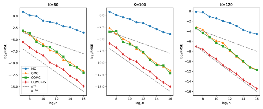
Figure 1: RMSEs for the single asset Asian option with $d=80$. The RMSEs are computed based on $100$ repetitions. The figure has two reference lines proportional to labeled powers of $n$.

In the numerical experiments for the single-asset arithmetic Asian option, we set the parameters as follows: initial asset price $S_{0}=100$, volatility $\sigma=0.4$, maturity $T=1$, dimension $d=80$, risk-free rate $r=0.1$, and strike prices $K\in\{80,100,120\}$. Root mean square errors (RMSE) are estimated based on 100 repetitions. We use the CQMC+IS method with a very large sample size to obtain a high-precision estimate, which is treated as the true value. GPCA is used as the path generation method throughout all the situations. We choose the sample sizes $n=2^{7},\dots,2^{16}$. Figures 1 show the RMSE of plain MC, plain QMC, CQMC, and CQMC+IS methods under different strike prices $K=80,100,120$ for $d=80$, respectively. It can be observed that the convergence rate of the CQMC+IS method closely matches the theoretical rate of $n^{-1}$. CQMC+IS achieves the lowest RMSE across all dimensions, leveraging preintegration and importance sampling to reduce variance. For $d=80$, QMC and CQMC perform better than MC but are outperformed by CQMC+IS, which effectively improves efficiency through conditional smoothing and dimension reduction.

5.1.2 Multi-assets

In this section, we study a multi-assets option, which is called the basket option. A basket option depends on a weighted average of several assets [17]. Suppose that under the risk-neutral measure the $L$ assets $S^{(1)},\ldots,S^{(L)}$ follow the SDE

$$\mathrm{d}S_{t}^{(\ell)}=rS_{t}^{(\ell)}\,\mathrm{d}t+\sigma_{\ell}S_{t}^{(\ell)}\,\mathrm{d}B_{t}^{(\ell)},$$

where $\{B^{(\ell)}\}_{1\leq\ell\leq L}$ are standard Brownian motions with correlation $Cov(B^{(l)}(s),B^{(k)}(t))=\rho\min(s,t)$ for all $t>0$ and $l,k~\in\{\ 1,2\dots L\}$. For some nonnegative weights $w_{1}+\cdots+w_{L}=1$, the payoff function of the Asian basket call option is given by

$$\left(\sum_{\ell=1}^{L}w_{\ell}\bar{S}^{(\ell)}-K\right)_{+},$$

where $\bar{S}^{(\ell)}$ is the arithmetic average of $S_{t}^{(\ell)}$ in the time interval $[0,T]$. Here, we only consider $L=2$ assets. To generate $B^{(1)},B^{(2)}$ with correlation $\rho$, we can generate two independent standard Brownian motions $W^{(1)},W^{(2)}$ and let $B^{(1)}=W^{(1)}$, $B^{(2)}=\rho W^{(1)}+\sqrt{1-\rho^{2}}W^{(2)}$. Following the same discretization as before, we can generate $\boldsymbol{z}\sim\mathcal{N}(0,I_{2d})$. Then for time steps $j=1,\ldots,d$, let

$$S_{j}^{(1)}=S_{0}^{(1)}\exp\left(\left(r-\frac{\sigma_{1}^{2}}{2}\right)j\Delta t+\sigma_{1}\left(\rho\sum_{k=1}^{d}A_{jk}z_{k+d}+\sqrt{1-\rho^{2}}\sum_{k=1}^{d}A_{jk}z_{k}\right)\right),$$ (29)

and

$$S_{j}^{(2)}=S_{0}^{(2)}\exp\left(\left(r-\frac{\sigma_{2}^{2}}{2}\right)j\Delta t+\sigma_{2}\sum_{k=1}^{d}A_{jk}z_{k+d}\right).$$ (30)

Then the payoff function becomes

$$e^{-rT}\left(\bar{S}-K\right)_{+},$$ (31)

where

$$\bar{S}=\frac{w_{1}}{d}\sum_{j=1}^{d}S_{j}^{(1)}+\frac{w_{2}}{d}\sum_{j=1}^{d}S_{j}^{(2)}.$$

Obviously, the payoff funtion of the option satisfies the assumption 10. We choose the cholesky decomposition to generate the matrix $A$. Thus, all coefficients preceding $z_{1}$ are positive, and Assumption 8 is thereby naturally satisfied. Next, we derive the preintegration expression of equation (31) with respect to $z_{1}$,

$$\mathbb{E}[e^{-rT}(\bar{S}-K)^{+}|\boldsymbol{z}_{-1}]=\int_{-\infty}^{+\infty}e^{-rT}(\bar{S}-K)_{+}1\{\bar{S}-K>0\}\varphi(z_{1})dz_{1}$$

$$= \int_{-\infty}^{+\infty}e^{-rT}(\frac{w_{1}}{d}\sum_{j=1}S_{j}^{(1)}+\frac{w_{2}}{d}\sum_{j=1}^{d}S_{j}^{(2)}-K)_{+}1\{z_{1}>\psi_{d}\}\varphi(z_{1})dz_{1}$$

$$= \frac{w_{1}}{d}\sum_{j=1}^{d}\exp\left(-rT+\frac{1}{2}\sigma_{1}^{2}(1-\rho^{2})A_{j1}^{2}+\left(r-\frac{\sigma_{1}^{2}}{2}\right)j\Delta t+\sigma_{1}\left(\rho\sum_{k=1}^{d}A_{jk}z_{k+d}+\sqrt{1-\rho^{2}}\sum_{k=1}^{d}A_{jk}z_{k}\right)\right)$$

$$\cdot (1-\Phi(\psi_{d}-\sigma_{1}\sqrt{1-\rho^{2}}A_{j1}))+e^{-rT}\left(\sum_{j=1}^{d}S_{j}^{(2)}-K\right)(1-\Phi(\psi_{d})).$$

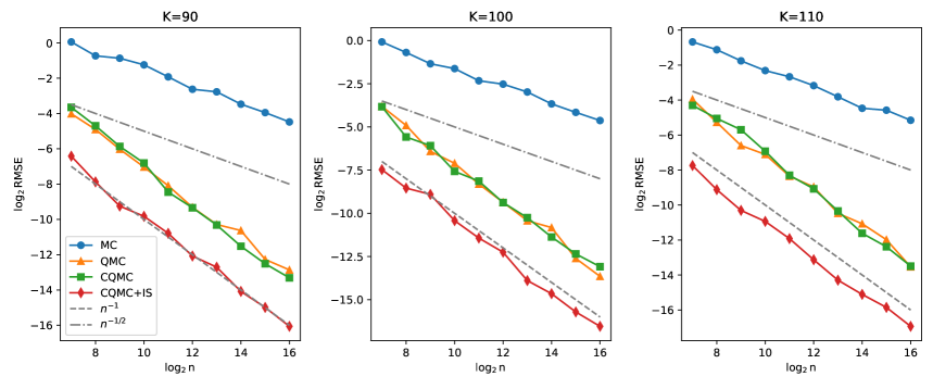
Figure 2: RMSEs for the multi-asset Asian option with $2d=30$. The RMSEs are computed based on $100$ repetitions. The figure has two reference lines proportional to labeled powers of $n$.

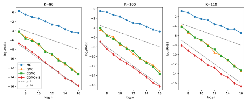
Figure 3: RMSEs for the multi-asset Asian option with $2d=60$. The RMSEs are computed based on $100$ repetitions. The figure has two reference lines proportional to labeled powers of $n$.

For the multi-asset basket option experiments, parameters are set as follows: initial prices of the two assets $S_{0}^{(1)}=S_{0}^{(2)}=100$, volatilities $\sigma_{1}=0.3$, $\sigma_{2}=0.1$, maturity $T=1$, weights $w_{1}=0.7$, $w_{2}=0.3$, dimensions $d=15,30$, risk-free rate $r=0.05$, strike prices $K\in\{90,100,110\}$, and correlation coefficient $\rho=0.5$. The nominal dimensions are $2d=30,60$. The root mean square errors are estimated based on 100 repetitions. We use the CQMC+IS method with a very large sample size to obtain an accurate estimation and treat it as the true value. GPCA is used as the path generation method throughout all the situations. We choose the sample sizes $n=2^{7},\dots,2^{16}$. Figures 2, 3 show the RMSE of plain MC, plain QMC, CQMC, and CQMC+IS methods under different strike prices $K=90,100,110$ for $d=15$ and $d=30$, respectively. It can be observed that the convergence rate of the CQMC+IS method closely matches the theoretical rate of $n^{-1}$. Notably, for out-of-the-money options (e.g., $K=110$), the variance reduction effect of IS is more pronounced: CQMC+IS achieves a significantly lower RMSE compared to other methods. This is because out-of-the-money scenarios involve rarer payoff events, and IS effectively targets these events, enhancing the efficiency of variance reduction. The weighted average structure of the basket option introduces additional complexity, but CQMC+IS still maintains the lowest RMSE. As the dimension increases (from $d=15$ to $d=30$), the performance gap between CQMC+IS and other methods widens: QMC and CQMC outperform MC but are surpassed by CQMC+IS, which handles multi-asset correlation and high-dimensionality through importance sampling and conditional smoothing.

5.2 Heston Model

Under the Heston framework, the risk-neutral dynamics of the asset can be expressed as

$$dS_{t}=rS_{t}dt+\sqrt{V_{t}}S_{t}dB^{(1)}_{t},$$ (32)

$$dV_{t}=(\theta-V_{t})\nu dt+\sigma\sqrt{V_{t}}dB^{(2)}_{t},$$ (33)

where $\nu$ is the mean-reversion parameter of the volatility process $V_{t}$, $\theta$ is the long run average price variance, $\sigma$ is the volatility of the volatility, $B^{(1)}_{t}$ and $B^{(2)}_{t}$ are two standard Brownian motions with an instantaneous correlation $\rho$, i.e., $Cov(B^{(1)}_{s},B^{(2)}_{t})=\rho\min(s,t)$ for any $s,t>0$. One may write that $B^{(1)}_{t}=\hat{\rho}W^{(1)}_{t}+\rho W^{(2)}_{t}$ and $B^{(2)}_{t}=W^{(2)}_{t}$, where $\hat{\rho}=\sqrt{1-\rho^{2}}$ and $W^{(1)}_{t}$ and $W^{(2)}_{t}$ are two independent standard Brownian motions. Let $\boldsymbol{z}=(z_{1},z_{2},\ldots,z_{2d-1},z_{2d})^{\mathrm{T}}\sim N(\boldsymbol{0},\boldsymbol{I}_{2d})$. We use the Euler-Maruyama scheme to discretize the asset paths [1], resulting in

$$S_{i}=S_{0}\exp\left\{ri\Delta t-\Delta t\sum_{j=0}^{i-1}V_{j}/2+\sqrt{\Delta t}\sum_{j=0}^{i-1}\sqrt{V_{j}}\bigl(\hat{\rho}z_{2j+1}+\rho z_{2j+2}\bigr)\right\},$$ (34)

$$V_{i}=V_{0}+\theta\nu i\Delta t-\nu\Delta t\sum_{j=0}^{i-1}V_{j}+\sigma\sqrt{\Delta t}\sum_{j=0}^{i-1}\sqrt{V_{j}}z_{2j+2}.$$ (35)

where $V_{0}$ is the initial value of the volatility process, $S_{i}$ and $V_{i}$ represent the approximations of $S_{i\Delta t}$ and $V_{i\Delta t}$ for $\Delta t=T/m$, respectively. Here we still consider estimating the price of an arithmetic average Asian call option

$$\mathbb{E}\bigl[e^{-rT}(S_{A}-K)^{+}\bigr],$$ (36)

where $S_{A}=(1/m)\sum_{i=1}^{m}S_{i}$.

Next, we provide the analytically expression for the preintegration of the payoff function with respect to $z_{1}$. Assumption 8 is satisfied, because all coefficients preceding $z_{1}$ are positive. The derivation is presented in [27].

$$\mathbb{E}\bigl[(S_{A}-K)^{+}\bigm|\boldsymbol{z}_{-1}\bigr]=\tilde{S}_{A}e^{(1-\rho^{2})V_{0}\Delta t/2}\bigl[1-\Phi\bigl(\psi_{d}(\boldsymbol{z}_{-1})-\hat{\rho}\sqrt{V_{0}\Delta t}\bigr)\bigr]-K\bigl[1-\Phi\bigl(\psi_{d}(\boldsymbol{z}_{-1})\bigr)\bigr],$$ (37)

where

$$\psi_{d}(\boldsymbol{z}_{-1})=\log(K/\tilde{S}_{A})/\sqrt{(1-\rho^{2})V_{0}\Delta t}.$$ (38)

$$\tilde{S}_{A}=(S_{0}/m)\sum_{i=1}^{m}\exp\left\{ri\Delta t-\Delta t\sum_{j=0}^{i-1}V_{j}/2+\rho\sqrt{\Delta tV_{0}}\,z_{2}+\sqrt{\Delta t}\sum_{j=1}^{i-1}\sqrt{V_{j}}\bigl(\hat{\rho}z_{2j+1}+\rho z_{2j+2}\bigr)\right\}.$$ (39)

Remark 2.

If the growth condition in Assumption 10 is modified to be controlled by $Le^{A\left|\boldsymbol{x}\right|^{r}}$, where $1\leq r<2$, then following the proof framework of Theorem 11 , it can be deduced that the preintegrated function is bounded by such an exponential function. In this case, the convergence order specified in Corollary 12 remains valid. Within the Heston model, the payoff function satisfies the aforementioned modified Assumption 10. Consequently, the convergence order can still be attained.

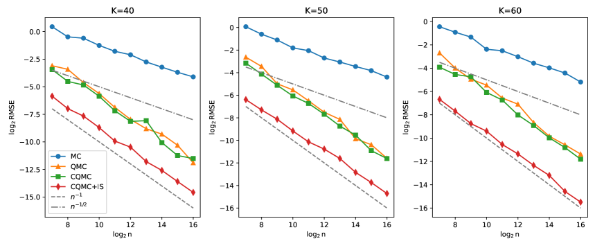
Figure 4: RMSEs for the Heston model with 2d=10. The RMSEs are computed based on 100 repetitions.The figure has two reference lines proportional to labeled powers of n.

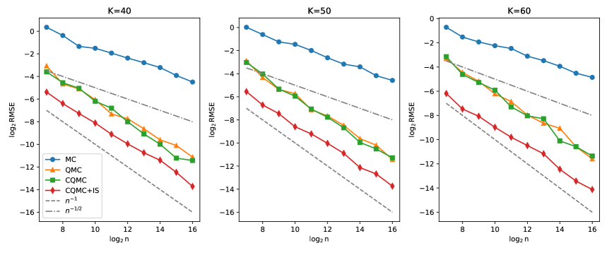
Figure 5: RMSEs for the Heston model with $2d=30$. The RMSEs are computed based on $100$ repetitions.The figure has two reference lines proportional to labeled powers of $n$.

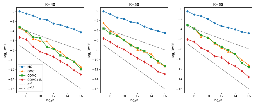
Figure 6: RMSEs for the Heston model with $2d=60$. The RMSEs are computed based on $100$ repetitions.The figure has two reference lines proportional to labeled powers of $n$.

In the numerical experiments, we choose $S_{0}=50$, $V_{0}=\theta=\sigma=0.2$, $T=1$, $\nu=1$, $d=5,15,30$, $r=0.05$, $K\in\{40,50,60\}$, and $\rho=0.5$. The nominal dimension is $2d=10,30,60$. The root mean square errors are estimated based on 100 repetitions. We use the CQMC+IS method with a very large sample size to obtain an accurate estimation and treat it as the true value. GPCA is used as the path generation method throughout all the situations. We choose the sample sizes $n=2^{7},\dots,2^{16}$. Figures 4, 5, 6 show the RMSE of plain MC, plain QMC, CQMC, and CQMC+IS methods under different strike prices $K=40,50,60$ for $d=5,d=15$ and $d=30$, respectively. It can be observed that the convergence rate of the CQMC+IS method closely matches the theoretical rate of $n^{-1}$. Stochastic volatility in the Heston model increases path complexity, but CQMC+IS still achieves the lowest RMSE across all dimensions, leveraging preintegration and importance sampling to handle volatility randomness. For $d=5,15,30$ (nominal dimension $2d=10,30,60$), QMC and CQMC perform better than MC but are outperformed by CQMC+IS, which effectively reduces variance through conditional smoothing and importance sampling.

6 Conclusion

In this paper, we addressed a significant gap in the convergence theory of Randomized Quasi-Monte Carlo with Importance Sampling (RQMC-IS), particularly for problems involving integrands with critical exponential growth. Standard theories require the growth rate exponent $A$ in $e^{A|\boldsymbol{x}|^{2}}$ to be strictly less than $1/2$, a condition that is often violated by practical and effective variance reduction techniques like Optimal Drift Importance Sampling (ODIS).

Our primary contribution is the development of a new, more general convergence theorem for RQMC-IS. This theorem extends the analysis to the critical case where $A=1/2$, establishing a near-$n^{-1}$ convergence rate under a verifiable light-tail condition on the proposal distribution. We then formally proved that the Gaussian proposals used in ODIS satisfy this condition, thus providing the first rigorous convergence guarantees for the widely used RQMC-ODIS method in these challenging scenarios.

Furthermore, we created a complete end-to-end framework for pricing complex financial derivatives. By integrating our new convergence theory with the preintegration technique, we demonstrated that even discontinuous payoff functions, once smoothed, can be efficiently estimated within our framework. We showed that if the components of the original payoff function have linear exponential growth, the smoothed function preserves this property, allowing it to be seamlessly combined with an IS proposal that introduces the critical quadratic exponential growth.

Numerical experiments on a variety of option pricing problems, including single-asset Asian, multi-asset basket, and stochastic volatility (Heston) models, empirically validated our theoretical findings. The results consistently demonstrated that our combined CQMC+IS method not only achieves the predicted convergence rate but also significantly outperforms standard MC, QMC, and CQMC methods in terms of accuracy and efficiency.

Future work could extend this work in several directions. One promising avenue is to investigate other families of proposal distributions beyond the Gaussian one, such as those with heavier tails, and analyze their compatibility with our theoretical framework. Another direction is to explore more practical applications of this methodology to other high-dimensional integration problems outside of finance, for example, in Bayesian statistics or computational physics.

Appendix A Appendix

This appendix provides detailed proofs for the key technical lemmas presented in the main text. We will prove lemma 6 by the mean value theorem, and calculate the $V_{HK}$ as in [20] to prove the lemma 5. They both need the following lemma about $\partial^{\boldsymbol{u}}(f_{IS})$. Thus, we begin by establishing a bound on the derivatives of the importance sampling integrand $f_{IS}$.

Lemma 13.

If $f/q$ as a function in $\mathcal{S}^{d}(\mathbb{R}^{d})$ satisfies the growth condition 12 and $\boldsymbol{u}\subseteq 1:d$, then

$$|\partial^{\boldsymbol{u}}f_{IS}(\boldsymbol{x})|\leq C(1+|\boldsymbol{x}|)^{|\boldsymbol{u}|}\exp\left(-\left(\frac{1}{2}-A\right)|\boldsymbol{x}|^{2}+B|\boldsymbol{x}|\right).$$

Proof.

By Leibniz rule, we have

$$\left|\partial^{\boldsymbol{u}}f_{IS}\right| =\left|\sum_{\boldsymbol{u}_{1}+\boldsymbol{u}_{2}=\boldsymbol{u}}\partial^{\boldsymbol{u}_{1}}\varphi\partial^{\boldsymbol{u}_{2}}\frac{f}{q}\right|$$

$$=\left|e^{-\frac{|\boldsymbol{x}|^{2}}{2}}\sum_{\boldsymbol{u}_{1}+\boldsymbol{u}_{2}=\boldsymbol{u}}\partial^{\boldsymbol{u}_{2}}\frac{f}{q}\prod_{j\in\boldsymbol{u}_{1}}(-x_{j})\right|$$

$$\leq e^{-\frac{|\boldsymbol{x}|^{2}}{2}}\sum_{\boldsymbol{u}_{1}+\boldsymbol{u}_{2}=\boldsymbol{u}}\left|\partial^{\boldsymbol{u}_{2}}\frac{f}{q}\right||\boldsymbol{x}|^{|\boldsymbol{u}_{1}|}$$

$$\leq e^{-\frac{|\boldsymbol{x}|^{2}}{2}}Ce^{A|\boldsymbol{x}|^{2}+B|\boldsymbol{x}|}\sum_{|\boldsymbol{u}_{1}|}|\boldsymbol{x}|^{|\boldsymbol{u}_{1}|}$$

$$=C(1+|\boldsymbol{x}|)^{|\boldsymbol{u}|}\exp\left\{-\left(\frac{1}{2}-A\right)|\boldsymbol{x}|^{2}+B|\boldsymbol{x}|\right\}.$$

∎

A.1 Proof of lemma 5

Proof.

By definition,

$$V_{HK}(f_{IS}\circ P_{R}\circ q^{-1})=\sum_{\varnothing\neq\boldsymbol{u}\subseteq 1:d}\int_{[0,1]^{d}}\left|\partial^{\boldsymbol{u}}(f_{IS}\circ P_{R}\circ q^{-1}(\boldsymbol{y}_{\boldsymbol{u}}:1_{-\boldsymbol{u}}))\right|\mathrm{d}\boldsymbol{y}.$$

By lemma 13, we have

$$\left|\partial^{\boldsymbol{u}}f\circ P_{R}\circ\Phi^{-1}(\boldsymbol{y}_{\boldsymbol{u}}:1_{-\boldsymbol{u}})\right|$$

$$= \left|\partial^{\boldsymbol{u}}f\left(P_{R}(\boldsymbol{x}_{\boldsymbol{u}}):P_{R}\circ\Phi^{-1}(1_{-\boldsymbol{u}})\right)\right|\cdot\left|\prod_{j\in\boldsymbol{u}}\frac{dP_{R}(\Phi^{-1}(y_{j}))}{d\Phi^{-1}(y_{j})}\frac{d\Phi^{-1}(y_{j})}{dy_{j}}\right|$$

$$\leq C(1+\sqrt{d}R)^{|\boldsymbol{u}|}e^{\sqrt{d}BR}\prod_{j\in\boldsymbol{u}}I_{\{|x_{j}|\leq R\}}\frac{1}{q(x_{j})}\mathrm{d}\boldsymbol{y},$$

where $x_{j}=q^{-1}(y_{j})$. Integrating both side and summing over all $\boldsymbol{u}$, we obtain that for $R>1$,

$$V_{HK}(f_{IS}\circ P_{R}\circ q^{-1}) \leq\sum_{\boldsymbol{u}\subseteq 1:d}C(1+\sqrt{d}R)^{|\boldsymbol{u}|}e^{\sqrt{d}BR}(2R)^{|\boldsymbol{u}|}$$

$$=Ce^{\sqrt{d}BR}\left(1+2R(1+\sqrt{d}R)\right)^{d}$$

$$\leq C(2\sqrt{d}+3)^{d}R^{2d}e^{\sqrt{d}BR}.$$ (40)

∎

A.2 Proof of lemma 6

Proof.

Let $H=[-(R-1),R-1]^{d}$ denote the hypercube in $\mathbb{R}^{d}$ with side length $2(R-1)$ centered at the origin. Then

$$E_{q}\left|f_{IS}(\boldsymbol{X})-f_{IS}\circ P_{R}(\boldsymbol{X})\right|^{2}=\int_{\mathbb{R}^{d}\setminus H}\left|f_{IS}(\boldsymbol{x})-f_{IS}\circ P_{R}(\boldsymbol{x})\right|^{2}q(\boldsymbol{x})\mathrm{d}\boldsymbol{x}.$$

Using the mean value theorem, we have

$$\left|f_{IS}(\boldsymbol{x})-f_{IS}\circ P_{R}(\boldsymbol{x})\right|\leq\left|\nabla f_{IS}(\boldsymbol{\xi}_{\boldsymbol{x}})\right|\cdot\left|\boldsymbol{x}-P_{R}(\boldsymbol{x})\right|,$$

where $\boldsymbol{\xi}_{\boldsymbol{x}}$ lies between $P_{R}(\boldsymbol{x})$ and $\boldsymbol{x}$. By lemma 13, we have

$$\left|\nabla f_{IS}(\boldsymbol{\xi}_{\boldsymbol{x}})\right|\leq\sqrt{d}C(1+|\boldsymbol{\xi}_{\boldsymbol{x}}|)\exp\left(B|\boldsymbol{\xi}_{\boldsymbol{x}}|\right).$$

Combing $|\boldsymbol{\xi}_{\boldsymbol{x}}|=|\lambda P_{R}(\boldsymbol{x})+(1-\lambda)\boldsymbol{x}|\leq|\boldsymbol{x}|$, we have

$$\left|f_{IS}(\boldsymbol{x})-f_{IS}\circ P_{R}(\boldsymbol{x})\right|^{2}\leq 4dC^{2}(1+|\boldsymbol{x}|)^{2}|\boldsymbol{x}|^{2}\exp\left(2A|\boldsymbol{x}|\right).$$

Integrating over $\mathbb{R}^{d}\setminus H$, we obtain

$$E_{q}\left|f_{IS}(\boldsymbol{X})-f_{IS}\circ P_{R}(\boldsymbol{X})\right|^{2} \leq 4dC^{2}\int_{\mathbb{R}^{d}\setminus H}(1+|\boldsymbol{x}|)^{2}|\boldsymbol{x}|^{2}\exp\left(2A|\boldsymbol{x}|\right)q(\boldsymbol{x})\mathrm{d}\boldsymbol{x}$$

$$=4dC^{2}E_{q}\left[(1+|\boldsymbol{X}|)^{2}|\boldsymbol{X}|^{2}e^{2A|\boldsymbol{X}|}I_{\mathbb{R}^{d}\setminus H}\right]$$

$$\leq 4dC^{2}E_{q}\left[(1+|\boldsymbol{X}|)^{2}|\boldsymbol{X}|^{2}e^{2A|\boldsymbol{X}|}I_{\{|\boldsymbol{X}|\geq R-1\}}\right]$$

$$\leq 16dC^{2}E_{q}\left[|\boldsymbol{X}|^{4}e^{2A|\boldsymbol{X}|}I_{\{|\boldsymbol{X}|\geq R-1\}}\right]$$

$$\leq 16dC^{2}C_{0}R^{\alpha}e^{-\beta R^{\gamma}}$$

for $R>2$, under the condition, we obtain the desired bound. For $1\leq R\leq 2$, we note that $R^{-\alpha}e^{\beta R^{\gamma}}E_{q}\left[(1+|\boldsymbol{X}|)^{2}|\boldsymbol{X}|^{2}e^{2A|\boldsymbol{X}|}I_{\{|\boldsymbol{X}|\geq R-1\}}\right]$ as a function of $R$ is continuous on $R\in[1,2]$, thus we can find a constant $C(\alpha,\beta,\gamma)$ such that

$$E_{q}\left[(1+|\boldsymbol{X}|)^{2}|\boldsymbol{X}|^{2}e^{2A|\boldsymbol{X}|}I_{\{|\boldsymbol{X}|\geq R-1\}}\right]\leq C(\alpha,\beta,\gamma)R^{\alpha}e^{\beta R^{\gamma}},$$

implying that

$$E_{q}\left|f_{IS}(\boldsymbol{X})-f_{IS}\circ P_{R}(\boldsymbol{X})\right|^{2}\leq 4dC^{2}C(\alpha,\beta,\gamma)R^{\alpha}e^{\beta R^{\gamma}}.$$

Therefore, for any $R>1$, we can find a constant $C_{1}$ such that

$$E_{q}\left|f_{IS}(\boldsymbol{X})-f_{IS}\circ P_{R}(\boldsymbol{X})\right|^{2}\leq C_{1}R^{\alpha}e^{\beta R^{\gamma}},$$

where $C_{1}$ is a constant depending on $\alpha$, $\beta$, and $\gamma$. This completes the proof. ∎

A.3 Proof of proposition 7

Proof.

Consider the integral

$$\int_{\mathbb{R}^{d}\setminus H}|\boldsymbol{x}|^{4}\exp\{2B|\boldsymbol{x}|\}q(\boldsymbol{x})\mathrm{d}\boldsymbol{x}.$$

For $R>4(|\mu|+2B)+1$, we have

$$|\boldsymbol{x}|\geq R-1\implies|\boldsymbol{x}-\boldsymbol{\mu}|\geq R-1-|\boldsymbol{\mu}|.$$

Thus,

$$\exp\left(-\frac{1}{2}|\boldsymbol{x}-\boldsymbol{\mu}|^{2}\right)\leq\exp\left(-\frac{1}{2}(R-1-|\boldsymbol{\mu}|)^{2}\right).$$

Therefore,

$$\int_{\mathbb{R}^{d}\setminus H}|\boldsymbol{x}|^{4}\exp\{2A|\boldsymbol{x}|\}q(\boldsymbol{x})\mathrm{d}\boldsymbol{x}\leq(2\pi)^{-d/2}\exp\left(-\frac{1}{2}|\boldsymbol{\mu}|^{2}\right)\int_{\mathbb{R}^{d}\setminus B(0,R-1)}|\boldsymbol{x}|^{4}\exp\left(-\frac{1}{4}|\boldsymbol{x}|^{2}\right)\mathrm{d}\boldsymbol{x}.$$

Evaluating the integral in spherical coordinates, we obtain

$$\int_{\mathbb{R}^{d}\setminus B(0,R-1)}|\boldsymbol{x}|^{4}\exp\left(-\frac{1}{4}|\boldsymbol{x}|^{2}\right)\mathrm{d}\boldsymbol{x}\leq\frac{(4+2)!!}{4\sqrt{\pi}}R^{3}e^{-\frac{R^{2}}{4}}.$$

Thus,

$$\int_{\mathbb{R}^{d}\setminus H}|\boldsymbol{x}|^{4}\exp\{2A|\boldsymbol{x}|\}q(\boldsymbol{x})\mathrm{d}\boldsymbol{x}\leq C\exp\left(-\frac{R^{2}}{4}\right),$$

which satisfies the condition for sufficiently large $R$. ∎

References

• [1] Nico Achtsis, Ronald Cools, and Dirk Nuyens. Conditional sampling for barrier option pricing under the Heston model. In Monte Carlo and Quasi-Monte Carlo Methods 2012, pages 253โ€“269. Springer, 2013.
• [2] Peterย A Acworth, Mark Broadie, and Paul Glasserman. A comparison of some Monte Carlo and quasi Monte Carlo techniques for option pricing. In Monte Carlo and Quasi-Monte Carlo Methods 1996: Proceedings of a conference at the University of Salzburg, Austria, July 9โ€“12, 1996, pages 1โ€“18. Springer, 2011.
• [3] Bย Owen Art. Monte Carlo theory, methods and examples, 2013.
• [4] Russelย E. Caflisch. Monte carlo and quasi-Monte Carlo methods. Acta Numerica, 7:1โ€“49, 1998.
• [5] Russelย E Caflisch, William Morokoff, and Art Owen. Valuation of mortgage-backed securities using brownian bridges to reduce effective dimension. Journal of Computational Finance, 1997.
• [6] Josef Dick and Friedrich Pillichshammer. Digital nets and sequences: discrepancy theory and quasi-Monte Carlo integration. Cambridge University Press, 2010.
• [7] Josef Dick, Daniel Rudolf, and Houying Zhu. A weighted discrepancy bound of quasi-Monte Carlo importance sampling. Statistics & Probability Letters, 149:100โ€“106, 2019.
• [8] Michael Fu and Jian-Qiang Hu. Conditional Monte Carlo gradient estimation, pages 73โ€“131. Springer US, 1997.
• [9] Paul Glasserman. Monte Carlo Methods in Financial Engineering, volumeย 53. Springer, 2004.
• [10] Paul Glasserman, Philip Heidelberger, and Perwez Shahabuddin. Asymptotically optimal importance sampling and stratification for pricing path-dependent options. Mathematical finance, 9(2):117โ€“152, 1999.
• [11] Michael Griebel, Frances Kuo, and Ian Sloan. The smoothing effect of integration in temp and the ANOVA decomposition. Mathematics of Computation, 82(281):383โ€“400, 2013.
• [12] Michael Griebel, Frances Kuo, and Ian Sloan. Note on โ€œthe smoothing effect of integration in temp and the ANOVA decompositionโ€. Mathematics of Computation, 86(306):1847โ€“1854, 2017.
• [13] Michael Griebel, Francesย Y. Kuo, and Ianย H. Sloan. The smoothing effect of the ANOVA decomposition. Journal of Complexity, 26(5):523โ€“551, 2010.
• [14] Andreas Griewank, Francesย Y. Kuo, Hernan Leรถvey, and Ianย H. Sloan. High dimensional integration of kinks and jumpsโ€”smoothing by preintegration. Journal of Computational and Applied Mathematics, 344:259โ€“274, 2018.
• [15] Zhijian He. On the error rate of conditional quasi-Monte Carlo for discontinuous functions. SIAM Journal on Numerical Analysis, 57(2):854โ€“874, 2019.
• [16] Anthonyย YC Kuk. Laplace importance sampling for generalized linear mixed models. 1999.
• [17] Sifan Liu and Artย B. Owen. Preintegration via active subspace. SIAM Journal on Numerical Analysis, 61(2):495โ€“514, 2023.
• [18] Jiล™รญ Matouลกek. On the $L^{2}$-discrepancy for anchored boxes. Journal of Complexity, 14(4):527โ€“556, 1998.
• [19] Harald Niederreiter. Random number generation and quasi-Monte Carlo methods. SIAM, 1992.
• [20] Duย Ouyang, Xiaoqun Wang, and Zhijian He. Achieving high convergence rates by quasi-Monte Carlo and importance sampling for unbounded integrands. SIAM Journal on Numerical Analysis, 62(5):2393โ€“2414, 2024.
• [21] Art Owen and Yiย Zhou. Safe and effective importance sampling. Journal of the American Statistical Association, 95(449):135โ€“143, 2000.
• [22] Artย B Owen. Randomly permuted (t, m, s)-nets and (t, s)-sequences. In Monte Carlo and Quasi-Monte Carlo Methods in Scientific Computing: Proceedings of a conference at the University of Nevada, Las Vegas, Nevada, USA, June 23โ€“25, 1994, pages 299โ€“317. Springer, 1995.
• [23] Artย B. Owen. Halton sequences avoid the origin. SIAM Review, 48(3):487โ€“503, 2006.
• [24] Artย B. Owen. Practical Quasi-Monte Carlo Integration. https://artowen.su.domains/mc/practicalqmc.pdf, 2023.
• [25] Yeย Xiao and Xiaoqun Wang. Enhancing quasi-Monte Carlo simulation by minimizing effective dimension for derivative pricing. Computational Economics, 54(1, SI):343โ€“366, 2019.
• [26] Chaojun Zhang and Xiaoqun Wang. Quasi-Monte Carlo-based conditional pathwise method for option greeks. Quantitative Finance, 20(1):49โ€“67, 2020.
• [27] Chaojun Zhang, Xiaoqun Wang, and Zhijian He. Efficient importance sampling in quasi-Monte Carlo methods for computational finance. SIAM Journal on Scientific Computing, 43(1):B1โ€“B29, 2021.