Bifurcations of viscous boundary layers in the half space

D. Bian, E. Grenier¹, G. Iooss

Abstract

It is well-established that shear flows are linearly unstable provided the viscosity is small enough, when the horizontal Fourier wave number lies in some interval, between the so-called lower and upper marginally stable curves. In this article, we prove that, under a natural spectral assumption, shear flows undergo a Hopf bifurcation near their upper marginally stable curve. In particular, close to this curve, there exists space periodic traveling waves solutions of the full incompressible Navier-Stokes equations. For the linearized operator, the occurrence of an essential spectrum containing the entire negative real axis causes certain difficulties which are overcome. Moreover, if this Hopf bifurcation is super-critical, these time and space periodic solutions are linearly and nonlinearly asymptotically stable.

1 Introduction

In this paper, we consider the incompressible Navier-Stokes equations in the half space $\Omega=\mathbb{R}\times\mathbb{R}_{+}$

$$\partial_{t}u^{\nu}+(u^{\nu}\cdot\nabla)u^{\nu}-\nu\Delta u^{\nu}+\nabla p^{\nu}=f^{\nu},$$ (1)

$$\nabla\cdot u^{\nu}=0,$$ (2)

together with the Dirichlet boundary condition

$$u^{\nu}=0\quad\hbox{when}\quad y=0$$ (3)

and address the classical question of the linear and nonlinear stability of shear flows for these equations.

A shear flow is a stationary solution of (1,2,3) of the form

$$U(y)=(U_{s}(y),0),\qquad f^{\nu}=(-\nu\Delta U_{s},0),$$

where $U_{s}(y)$ is a smooth function, vanishing at $y=0$ and converging exponentially fast at infinity to some constant $U_{+}$.

The question of the linear stability of such shear flows is one of the most classical questions in Fluid Mechanics, which has been intensively studied since the pioneering work of Lord Rayleigh at the end of the $19^{th}$ century. The situation has been progressively understood in the $20^{th}$ century thanks to the works of L. Prandtl, Orr, Sommerfeld, Schlichting and C.C. Lin to only quote a few names. We in particular refer to [8, 15, 16] for a detailed presentation of the approach in physics.

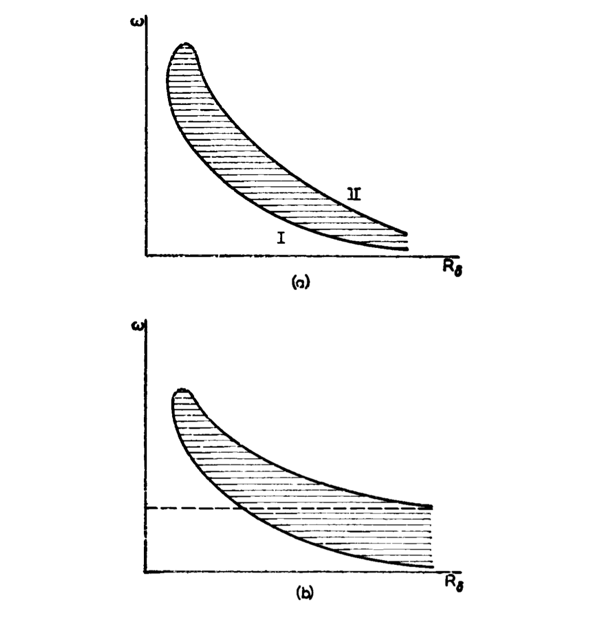
Figure 1: Stability of shear flows: horizontally, the Reynolds number (inverse of $\nu$), vertically the horizontal wave length $\alpha$ of the perturbation. In grey, the unstable area. Top sub-figure: Euler-stable profile. Bottom sub-figure: Euler-unstable profile. From [14].

Roughly speaking, shear flows can be classified into two categories:

• Some are spectrally unstable for the Euler equations, namely in the case $\nu=0$ (see the bottom sub-figure of Figure 1). According to Rayleigh criterium, such shear flows have inflection points.

• Other are spectrally stable for the Euler equations, which is the case if they have no inflection points, for instance if they are convex or concave (see the top sub-figure of Figure 1).

In both cases, provided the Reynolds number is large enough, namely provided the viscosity $\nu$ is small enough, the shear layer is linearly unstable with respect to perturbations whose horizontal wavenumber $\alpha$ lies in some interval $[\alpha_{-}(\nu),\alpha_{+}(\nu)]$ for some increasing functions $\alpha_{\pm}(\nu)$. The function $\alpha_{-}(\nu)$ (respectively $\alpha_{+}(\nu)$) is called the lower (respectively upper) marginal stability curve.

Let us fix $\nu=\nu_{0}$ small enough, which corresponds to a large enough Reynolds number. Then if $\alpha>\alpha_{+}(\nu_{0})$, we note that the harmonics of $\alpha$, namely all the positive multiple of $\alpha$, remain larger than the basic harmonic $\alpha_{+}(\nu_{0})$ and thus are all stable. As a consequence, we expect that the shear layer $U$ is linearly and nonlinear stable with respect to perturbations which are $2\pi/\alpha$ periodic.

However, if $\alpha<\alpha_{+}(\nu_{0})$ and close to $\alpha_{+}(\nu_{0})$, a linear instability appears and, following [16] (section $5.3$), we expect a bifurcation: small perturbations will grow exponentially till the nonlinear term saturates them, leading to a bifurcated solution, which is a traveling wave of small amplitude.

The aim of this article is to investigate mathematically this physical scenario. We first formalize the spectral situation depicted on Figure 1, which leads to the following set of assumptions and then study the bifurcation arising at $\alpha_{+}(\nu)$.

We take the Fourier transform in the $x$ variable, with dual Fourier variable $\alpha$. We denote by $Sp_{\alpha,\nu}$ the spectrum of the linearized Navier-Stokes equations after this Fourier transform, and by $\lambda(\alpha,\nu)\in Sp_{\alpha,\nu}$ the eigenvalue (if it exists and is unique) with the largest real part.

In this article, we assume that, when the viscosity $\nu$ is small enough, there exist two smooth and increasing functions $\alpha_{\pm}(\nu)$, defined for $\nu$ small enough, with $\alpha_{-}(\nu)<\alpha_{+}(\nu)$, such that

• for $\alpha_{-}(\nu)<|\alpha|<\alpha_{+}(\nu)$, $\lambda(\alpha,\nu)$ exists, is unique, and satisfies

  $$\Re\lambda(\alpha,\lambda)>0.$$

  Moreover, $\lambda$ is simple, with corresponding eigenvector $\zeta(x,y)$ of the form

  $$\zeta(x,y)=\nabla^{\perp}\Bigl[e^{i\alpha x}\psi_{\alpha,\nu}(y)\Bigr],$$

  for some smooth stream function $\psi_{\alpha,\nu}(y)$ which is exponentially decreasing at infinity,

• for $|\alpha|>\alpha_{+}(\nu)$, close to $\alpha_{+}(\nu)$, $\lambda(\alpha,\nu)$ exists, is unique and satisfies

  $$\Re\lambda(\alpha,\nu)<0,$$

• for $|\alpha|=\alpha_{+}(\nu)$, $\lambda(\alpha,\nu)$ is well defined and purely imaginary. Moreover, defining $\nu_{0}(\alpha)$ by $\alpha=\alpha_{+}(\nu_{0})$

  $$(\partial_{\nu}\Re\lambda)(\alpha,\nu)|_{\nu=\nu_{0}(\alpha)}>0.$$

The mathematical proof of the existence of an unstable mode for some values of $\alpha$ has been initiated in [9], where it is established that any shear flow is spectrally unstable for the incompressible Navier-Stokes equations provided the viscosity is small enough, a first result later improved by [6] and [2]. In this last paper, we proved that strictly convex or concave flows satisfy the set of assumptions (A1), (A2) and (A3) under the additional assumptions $U_{s}^{\prime}(0)\neq 0$ and $U_{+}\neq 0$.

When we cross the upper marginally stable curve $\alpha=\alpha_{+}(\nu)$, two eigenvalues cross the imaginary axis (corresponding to $\pm\alpha$): we are exactly in the situation of an Hopf bifurcation. This paper focuses on the study of this bifurcation.

Let us now state our main result in an informal way. We refer to Theorems 18, 22 and 27 for detailed statements, including precise definitions of the function spaces.

Theorem 1.

Let us assume (A1), (A2) and (A3). Let $\nu_{0}>0$ and let $\alpha=\alpha_{+}(\nu_{0})$, let us consider perturbations which are $2\pi/\alpha$ periodic in $x$. Then, at $\nu=\nu_{0}$, the system undergoes a Hopf bifurcation:

• for $\nu<\nu_{0}$, the shear flow $U$ is linearly and nonlinearly stable,

• if the Hopf bifurcation is subcritical, there exists a time and space periodic solution of (1,2,3) for $\nu<\nu_{0}$ sufficiently close to $\nu_{0}$, and this time and space periodic solution is linearly unstable,

• if the Hopf bifurcation is supercritical, there exists a time and space periodic solution of (1,2,3) for $\nu>\nu_{0}$, sufficiently close to $\nu_{0}$, and this time and space periodic solution is linearly and nonlinearly stable.

There exist many works dealing with Hopf bifurcations on Navier-Stokes equations (see [11] for detailed references), however, all these works consider bounded domains or periodic domains (for Couette-Taylor flow [7] or Bénard-Rayleigh convection for example). Recently, some works deal with parallel flows, like for example Poiseuille flow in [5] at section $6.4$, where a sub-critical Hopf bifurcation of a traveling wave is completely treated (see also [1] for the Hopf bifurcation of a shear flow between two plates).

None of these works deal with an half plane domain ($x\in\mathbb{R},y\in\mathbb{R}^{+}$), assuming periodicity only in the $x$ direction, the $y$ direction being unbounded, which is a problem of serious physical interest. As the domain is unbounded in the $y$ direction, the essential spectrum of the linearized operator goes up to zero and there is no spectral gap. The classical tools of bifurcation theory cannot be applied and we have to design a new approach. Moreover, in cases where the shear flow $U$ is stable, perturbation do not decay exponentially fast, but only like polynomially fast, as $t^{-1}$.

The super-criticality or sub-criticality of the Hopf bifurcation depends on the sign of a coefficient which unfortunately can only be numerically studied. In the case of exponential profiles $U_{s}(y)=1-e^{-y}$, numerical evidence [3] indicates that the Hopf bifurcation is supercritical.

The paper is organized as follows: in section $2$, we introduce the various function spaces, the various linear operators and investigate their spectra and their related semi-groups. In section $3$ we prove the nonlinear stability of the shear flow $U$ above the upper marginal stability curve. In section $4$ we investigate the bifurcation and prove the existence of a traveling wave, time periodic solution to the Navier Stokes equations. In section $5$, we focus on the linear and non linear stability of this periodic solution. The proofs of the various lemmas are detailed in the Appendix.

Notations

In all this paper, $\eta$ will be a sufficiently small positive number. We define the one-dimensional periodic torus of period $2\pi/\alpha$ to be $\mathbb{T}=\mathbb{R}/(2\pi/\alpha)\mathbb{Z}$. We define the Banach space $C^{0}_{\eta}(\mathbb{R}^{+})$ by its norm

$$\|u\|_{C_{\eta}^{0}}=\underset{y\in\mathbb{R}^{+}}{\sup}|u(y)e^{\eta y}|.$$

The components of a two dimensional vector field $v$ will be denoted by $v=(v^{x},v^{y})$. We denote by $D$ the derivative with respect to $y$. We denote by $u_{n}(y)$ the $n^{th}$ Fourier component of a function $u(x,y)$.

By a slight abuse of language, we will also denote the vector $(U_{+},0)$ by $U_{+}$.

2 Preliminaries

2.1 Function spaces

We first observe that if $v=(v^{x},v^{y})$ is a two dimensional divergence free vector field which is independent on $x$ and vanishes at $y=0$, then, using the incompressibility condition, $v^{y}=0$.

Let us define the Banach space

$$\mathcal{X}_{\eta}=\mathring{L}_{\eta}^{2}\oplus\mathring{L}^{\infty},$$

so that $v\in\mathcal{X}_{\eta}$ can be written as

$$v = \widetilde{v}+v_{0},\text{ }\widetilde{v}\in\mathring{L}_{\eta}^{2},$$

$$v_{0} = (v_{0}^{x},0),\text{ }v_{0}^{x}\in L^{\infty}(\mathbb{R}^{+}),$$

where we define

$$\mathring{L}_{\eta}^{2}=\Bigl\{\widetilde{v}\in L_{\eta}^{2};\,\nabla\cdot\widetilde{v}=0,\,\widetilde{v}^{y}|_{y=0}=0\Bigr\},$$

with

$$L_{\eta}^{2}=\Bigl\{\widetilde{u}\in[L^{2}[\mathbb{T},C_{\eta}^{0}(\mathbb{R}^{+})]]^{2};\,\int_{0}^{2\pi/\alpha}\widetilde{u}(x,y)\,dx=0,\text{ }\|\widetilde{u}\|_{L_{\eta}^{2}}<\infty\Bigr\},$$

$$\mathring{L}^{\infty}=\Bigl\{(v_{0}^{x},0);\,v_{0}^{x}\in L^{\infty}(\mathbb{R}^{+})\Bigr\},$$

$$\|\widetilde{u}\|_{L_{\eta}^{2}}^{2} = \sum_{|n|\geq 1}\|u_{n}\|_{C_{\eta}^{0}}^{2},$$

$$\|v_{0}\|_{\mathring{L}^{\infty}} = \|v_{0}^{x}\|_{L^{\infty}}.$$

Note that we do not assume any decay in $y$ on the 0-Fourier mode $v_{0}$. By analogy, we define the Banach spaces $H_{\eta}^{2},$ $\mathring{H}_{\eta}^{2}$ and

$$\mathcal{Z}_{\eta}=\mathring{H}_{\eta}^{2}\oplus\mathring{W}^{2,\infty},$$

where

$$\mathring{H}_{\eta}^{2}=\Bigl\{\widetilde{v}\in H_{\eta}^{2};\,\nabla\cdot\widetilde{v}=0,\,\widetilde{v}|_{y=0}=0,\,\|\widetilde{v}\|_{\mathring{H}_{\eta}^{2}}<\infty\Bigr\},$$

$$H_{\eta}^{2} = \Bigl\{\widetilde{u}\in[H^{2}[\mathbb{T},C_{\eta}^{2}(\mathbb{R}^{+})]]^{2};\,\int_{0}^{2\pi/\alpha}\widetilde{u}(x,y)\,dx=0,\,\|\widetilde{u}\|_{H_{\eta}^{2}}<\infty\Bigl\},$$

$$\mathring{W}^{2,\infty}=\Bigl\{(v_{0}^{x},0);\,v_{0}^{x}|_{y=0}=0,\,v_{0}^{x}\in W^{2,\infty}(\mathbb{R}^{+})\Bigr\},$$

with the corresponding norms

$$\|\widetilde{v}\|_{H_{\eta}^{2}}^{2}=\sum_{|n|\geq 1}\|D^{2}v_{n}\|_{C_{\eta}^{0}}^{2}+n^{2}\|Dv_{n}\|_{C_{\eta}^{0}}^{2}+n^{4}\|v_{n}\|_{C_{\eta}^{0}}^{2}$$

and

$$\|v_{0}\|_{\mathring{W}^{2,\infty}}=\|v_{0}^{x}\|_{W^{2,\infty}},$$

so that $\mathcal{Z}_{\eta}\mathcal{\hookrightarrow X}_{\eta}$ densely.

We also define the intermediary Banach space

$$\mathcal{Y}_{\eta}=\mathring{H}_{\eta}^{1}\oplus\mathring{W}^{1,\infty}\hookrightarrow\mathcal{X}_{\eta},$$

with

$$\mathring{H}_{\eta}^{1} = \Bigl\{\widetilde{v}\in[H^{1}[\mathbb{T},C_{\eta}^{1}(\mathbb{R}^{+})]]^{2};$$

$$\quad\int_{0}^{2\pi/\alpha}\widetilde{v}(x,y)\,dx=0,\text{ }\nabla\cdot\widetilde{v}=0,\widetilde{v}^{y}|_{y=0}=0,\text{ }\|\widetilde{v}\|_{\mathring{H}_{\eta}^{1}}<\infty\Bigr\},$$

$$\mathring{W}^{1,\infty}=\Bigl\{(v_{0}^{x},0);\,v_{0}^{x}\in W^{1,\infty}(\mathbb{R}^{+})\Bigr\}$$

and the norm

$$\|\widetilde{v}\|_{\mathring{H}_{\eta}^{1}}^{2}=\sum_{|n|\geq 1}n^{2}\|v_{n}\|_{C_{\eta}^{0}}^{2}+\|Dv_{n}\|_{C_{\eta}^{0}}^{2}.$$

2.2 The Helmholtz decomposition in $\mathcal{X}_{\eta}$

Let $u\in L_{\eta}^{2}\oplus(L^{\infty})^{2}$. Then $u$ can be decomposed in $u=\widetilde{u}+u_{0}$ with $\widetilde{u}\in L_{\eta}^{2}$ and $u_{0}\in[L^{\infty}(\mathbb{R}^{+})]^{2}$. We further decompose $\widetilde{u}$ in

$$\widetilde{u}=\widetilde{v}+\nabla\widetilde{\phi}$$

with $\widetilde{v}\in\mathring{L}_{\eta}^{2}$ and

$$\Delta\widetilde{\phi}=\nabla\cdot\widetilde{u},\quad\frac{\partial\widetilde{\phi}}{\partial y}|_{y=0}=\widetilde{u}^{y}|_{y=0}\in L^{2}(\mathbb{T}),$$

where $\nabla\cdot\widetilde{u}$ is understood in the distribution sense. The component $u_{0}$ can be decomposed as

$$u_{0} = \binom{v_{0}^{x}}{0}+\binom{0}{D\phi_{0}},\text{ }\binom{v_{0}^{x}}{0}\in\mathring{L}^{\infty},$$

with $D\phi_{0}=u_{0}^{y}\in L^{\infty}(\mathbb{R}^{+})$, so that $\widetilde{v}+v_{0}\in\mathcal{X}_{\eta}$. We note that $v_{0}$ and $\phi_{0}$ are independent of $x$. We now define the projection $\Pi$ on divergence free vector fields by

Lemma 2.

Let $\eta<\alpha/2$. Let $u\in L_{\eta}^{2}\oplus(L^{\infty})^{2}$, which may be decomposed in

$$u=\widetilde{u}+u_{0},\text{ }\widetilde{u}\in L_{\eta}^{2},\text{ }u_{0}\in(L^{\infty}(\mathbb{R}^{+}))^{2}.$$

We can further decompose $\widetilde{u}$ in $\widetilde{u}=\widetilde{v}+\widetilde{\nabla\phi}$ where $\widetilde{v}\in\mathring{L}_{\eta}^{2}$. We define the projection $\Pi u$ by

$$\Pi u=\Pi\widetilde{u}+(\Pi u)_{0}$$

where $\Pi\widetilde{u}=\widetilde{v}$ and $(\Pi u)_{0}=(v_{0}^{x},0)$. The projection $\Pi$ is bounded from $L_{\eta}^{2}$ to $\mathring{L}_{\eta}^{2}$ and from $(L^{\infty})^{2}$ to $\mathring{L}^{\infty}$

The projector $\Pi$ is highly classical, however our function spaces are not the usual ones. We thus detail the proof of this Lemma in Appendix 6.1.

2.3 Linear operators

We define the linear operators $\bm{L}_{(\nu)},\bm{L}^{(0)}_{(\nu)},\bm{L}^{(1)}$ by

$$\bm{L}_{(\nu)} =\bm{L}_{(\nu)}^{(0)}+\bm{L}^{(1)},$$

$$\bm{L}_{(\nu)}^{(0)}v =\nu\Pi\Delta v,\quad\bm{L}^{(1)}v=-\Pi\Bigl[(U\cdot\nabla)v+(v\cdot\nabla)U\Bigr],$$

and further decompose $\bm{L}_{(\nu)}^{(0)}$ in

$$\bm{L}_{(\nu)}^{(0)}=\bm{L}^{(0)}+(\nu-\nu_{0})\bm{L}^{\prime}$$

with

$$\bm{L}^{(0)}v =\nu_{0}\Pi\Delta v,\text{ }\bm{L}^{\prime}v=\Pi\Delta v.$$

Note that $\bm{L}^{\prime}$ and $\bm{L}^{(0)}_{(\nu)}$ are Stokes operators. We easily obtain the following Lemma.

Lemma 3.

Assume that $U\in C^{1}(\mathbb{R}^{+})$ with

$$|U(y)|+|DU(y)|\leq M<\infty,\text{ \ }y\in\mathbb{R}^{+},$$

then the linear operator $\bm{L}^{(1)}$ cancels on $\mathring{W}^{1,\infty}$. For $\eta<\alpha/2$ and $v=\widetilde{v}+v_{0}\in\mathcal{Z}_{\eta}$ with $\widetilde{v}\in\mathring{H}_{\eta}^{2},$ $v_{0}\in\mathring{W}^{2,\infty},$ then

$$\bm{L}^{(1)}v=\bm{L}^{(1)}\widetilde{v}\in\mathring{H}_{\eta}^{1}.$$

Moreover for $u\in\widetilde{u}+u_{0}\in\mathcal{Y}_{\eta}$ with $\widetilde{u}\in\mathring{H}_{\eta}^{1},$ $u_{0}\in\mathring{W}^{1,\infty},$ then

$$\bm{L}^{(1)}u=\bm{L}^{(1)}\widetilde{u}\in\mathring{L}_{\eta}^{2}.$$

There exists $C>0$ such that we have the estimates

$$\|\bm{L}^{(1)}v\|_{\mathring{H}_{\eta}^{1}}\leq C\|\widetilde{v}\|_{\mathring{H}_{\eta}^{2}},$$

$$\|\bm{L}^{(1)}u\|_{\mathring{L}_{\eta}^{2}}\leq C\|\widetilde{u}\|_{\mathring{H}_{\eta}^{1}}.$$

The main observation is that

$$(U\cdot\nabla)v+(v\cdot\nabla)U=U_{s}\partial_{x}v+\binom{v^{y}DU_{s}}{0},$$

cancels when $v$ is independent of $x$ and $v^{y}=0,$ which is the case in $\mathring{W}^{1,\infty}.$

2.4 Study of $\bm{L}_{(\nu)}^{(0)}$ and $\bm{L}_{(\nu)}$

We now turn to the study of the spectrum and of the resolvent of the operator $\bm{L}^{(0)}_{(\nu)}$. This operator is the classical Stokes operator, however our spaces are not the usual ones, thus we have to restart its study from the beginning.

Lemma 4.

The spectrum of $\bm{L}_{(\nu)}^{(0)}=\Pi\nu\Delta$ acting in $\mathring{L}^{\infty}$ is only formed by an essential spectrum which equals

$$Sp|_{\mathring{L}^{\infty}}\,\bm{L}_{(\nu)}^{(0)}=(-\infty,0]=\mathbb{R}^{-},$$

and we have the estimates

$$\Bigl\|(\bm{L}_{(\nu)}^{(0)}-\lambda\mathbb{I)}^{-1}\Bigr\|_{\mathcal{L}(\mathring{L}^{\infty})}\leq\left\{\begin{array}[]{ll}\sqrt{2}|\lambda|^{-1}&\text{when }\Re\lambda\geq 0,\\ (|\lambda|\cos\theta/2)^{-1}&\text{when }\lambda=|\lambda|e^{i\theta}\text{ with }\Re\lambda<0.\end{array}\right.$$

For $\lambda\in(-\infty,0],$ the range of the operator $\bm{L}_{(\nu)}^{(0)}-\lambda\mathbb{I}$ is not closed in $\mathring{L}^{\infty}$.

Now consider the linear operator $\bm{L}_{(\nu)}^{(0)}=\Pi\nu\Delta$ acting in $\mathring{L}_{\eta}^{2}$ . For any $\delta>0$ such that $0<\delta<\pi/6,$ and $\lambda\in\mathbb{C}$ such that

$$0 \leq |\arg(\lambda+\nu\alpha^{2})|\leq\frac{2\pi}{3}-\delta,$$

$$0 < \varepsilon_{0}\leq|\lambda+\nu\alpha^{2}|,$$

there exists $C>0$ such that, for $\eta>0$ small enough,

$$\Bigl\|(\bm{L}_{(\nu)}^{(0)}-\lambda\mathbb{I)}^{-1}\Bigr\|_{\mathcal{L}(\mathring{L}_{\eta}^{2})}\leq\frac{C}{|\lambda+\nu\alpha^{2}|}.$$ (4)

The spectrum of $\bm{L}_{(\nu)}^{(0)}$ on ${\mathring{L}_{\eta}^{2}}$ is thus contained in an angular sector of $\mathbb{C}$ defined by

$$\frac{2\pi}{3}\leq|\arg(\lambda+\nu\alpha^{2})|\leq\pi.$$

The proof of this Lemma is detailed in Appendix 6.2.

Remark 5.

If we chose to include the exponential decay $e^{-\eta y}$ for the $0$-Fourier mode, this would imply that

$$Sp|_{\mathring{L}_{\eta}^{\infty}}\,\bm{L}_{(\nu)}^{(0)}\subset\Bigl\{\lambda\in\mathbb{C};\,|\Im\lambda|\leq 4\nu\eta^{2}(\nu\eta^{2}-\Re\lambda)\Bigr\}$$

which is a parabolic region centered on, and containing, the negative real axis, bounded on the right side by $\Re\lambda=\nu\eta^{2}.$

Moreover, we have the following corollaries.

Lemma 6.

The linear operator $\bm{L}_{(\nu)}^{(0)}=\Pi\nu\Delta$ acting in $\mathring{L}_{\eta}^{2}$ has a bounded inverse in $\mathcal{L}(\mathring{L}_{\eta}^{2},\mathring{H}_{\eta}^{2}).$ In $\mathring{H}_{\eta}^{2}$, the norms $\|\cdot\|_{\mathring{H}_{\eta}^{2}}$ and $\|\bm{L}_{(\nu)}^{(0)}\cdot\|_{\mathring{L}_{\eta}^{2}}$ are equivalent.

This Lemma is a direct consequence of Lemma 4 since

$$\|\widetilde{v}\|_{\mathring{H}_{\eta}^{2}}\leq M\|\bm{L}^{(0)}_{(\nu)}\widetilde{v}\|_{\mathring{L}_{\eta}^{2}}\leq Mc\|\Delta\widetilde{v}\|_{\mathring{L}_{\eta}^{2}}\leq Mc\|\widetilde{v}\|_{\mathring{H}_{\eta}^{2}}.$$

Lemma 7.

There exists $M>0$ such that the spectrum of $\bm{L}_{(\nu)}$ is included in

$$\Bigl\{|\lambda+\nu\alpha^{2}|\leq M\Bigr\}\cup\Bigl\{\frac{2\pi}{3}\leq|\arg(\lambda+\nu\alpha^{2})|\leq\pi\Bigr\}\cup(-\infty,0].$$

Let $\delta>0$ be arbitrarily small. In the domain, $|\lambda+\nu\alpha^{2}|>M$ and $0\leq|\arg(\lambda+\nu\alpha^{2})|\leq 2\pi/3$, we have

$$\Bigl\|(\bm{L}_{(\nu)}-\lambda\mathbb{I)}^{-1}\Bigr\|_{\mathcal{L}(\mathring{L}_{\eta}^{2})}\leq\frac{C}{|\lambda|}.$$ (5)

We detail the proof of this lemma in Appendix 6.3.

We now decompose $L^{(1)}$ in

$$L^{(1)}=L^{(1,0)}+L^{(1,c)},$$

where

$$L^{(1,0)}v=-\Pi\Bigl[(U_{+}\cdot\nabla)v\Bigr],\qquad L^{(1,c)}v=-\Pi\Bigl[\Bigl((U-U_{+})\cdot\nabla\Bigr)v+(v\cdot\nabla)U\Bigr].$$

Lemma 8.

Assume that $U\in C^{2}(\mathbb{R}^{+})$ satisfies

$$|U(y)-U_{+}|+|DU(y)|+|D^{2}U(y)|\leq ce^{-\gamma y},\text{ }y\in\mathbb{R}^{+},$$

then the linear operator $\bm{L}^{(1,c)}$ is relatively compact with respect to $\bm{L}_{(\nu)}^{(0)}$ acting in $\mathcal{X}_{\eta}.$

This Lemma is proved in Appendix 6.4 (see [13] for the definition of relative compactness of an operator with respect to another operator).

Lemma 9.

The essential spectrum of $L_{(\nu)}$ is the essential spectrum of $L_{(\nu)}^{(0)}+L^{(1,0)}$. It is the half line $(-\infty,0]$ if restricted to $\mathring{L}^{\infty}.$ The rest of the essential spectrum, for the operator restricted to $\mathring{L}_{\eta}^{2},$ is included in the region $\Sigma_{U_{+}}$ defined by

$$\Re\lambda<-\nu(\alpha^{2}-\eta^{2}),$$

and either

$$\Re\lambda<-{\nu(\Im\lambda)^{2}\over U_{+}^{2}+4\nu^{2}\eta^{2}}+\nu\eta^{2}$$

or

$$2\pi/3\leq|\arg(\lambda+\nu\alpha^{2})|\leq\pi.$$

The rest of the spectrum of $L_{(\nu)}=L_{(\nu)}^{(0)}+L^{(1)}$ is uniquely formed by isolated eigenvalues with finite multiplicities at finite distances of $0$. See Figure 2.

Proof.

The localization of the essential spectrum of $L_{(\nu)}^{(0)}+L^{(1,0)}$ is proved in Appendix 6.5. The result on the spectrum of $\bm{L}_{(\nu)}$ comes from the fact that it is the addition to $\bm{L}^{(0)}_{(\nu)}+L^{(1,0)}$ of the linear operator $\bm{L}^{(1,c)}$ which is a relatively compact perturbation, using the fact that $U(y)-U_{+}$ tends to 0 exponentially as $y\rightarrow\infty$. We then apply theorem 5.35 in [13]. ∎

A corollary of the previous Lemmas is the following estimate for $\lambda$ on the imaginary axis, far enough from the origin. This estimate will be useful in the study of bifurcating periodic solutions.

Lemma 10.

Assume $\omega>0$ and $\eta>0$ small enough, then there exists $C>0$ and $N>0$ such that for $|n|>N$

$$\Bigl\|(in\omega-\bm{L}_{(\nu)})^{-1}\Bigr\|_{\mathcal{L}(\mathcal{X}_{\eta})}\leq\frac{C}{|n|}.$$

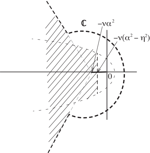
Figure 2: a) Location of the spectrum of $\bm{L}_{(\nu)}$ inside the region bounded by dashed line b) Location of the essential spectrum in the hatched region $\Sigma_{U_{+}}$ and on half left real line.

2.5 Semi-groups

For the study of the linear and nonlinear stabilities of the basic flow $U,$ we need to understand the behavior of the semi-group $e^{\bm{L}_{(\nu)}t}$ for $t>0.$ We start with estimates on the Stokes flow.

Lemma 11.

Let $\eta>0$ be small enough. Assume $0<\delta<\pi/6.$ The linear operator $\bm{L}_{(\nu)}^{(0)}$ is the infinitesimal generator of a bounded semi-group $e^{\bm{L}_{(\nu)}^{(0)}t}$ in $\mathcal{L}(\mathcal{X}_{\eta})$ which is holomorphic for $t\in\mathbb{C}$ in a sector of angle $\pi/3-2\delta$ centered on $\mathbb{R}^{+}.$ Moreover there exists $C>0$ such that for any $t\geq 0$,

$$\|e^{\bm{L}_{(\nu)}^{(0)}t}\|_{\mathcal{L}(\mathring{L}_{\eta}^{2})} \leq Ce^{-\nu\alpha^{2}t},$$

$$\|e^{\bm{L}_{(\nu)}^{(0)}t}\|_{\mathcal{L}(\mathring{L}^{\infty})} \leq C.$$ (6)

Proof.

This Lemma follows from the estimate (5) and from classical results on holomorphic semi-groups (see [13]). ∎

Now the operator $\bm{L}_{(\nu)}$ is a perturbation of $\bm{L}_{(\nu)}^{(0)}$ with the same essential spectrum as $\bm{L}_{(\nu)}^{(0)}+\bm{L}^{(0,1)}$, and with possible eigenvalues in a region bounded by the dashed curve in Figure 2. By assumptions (A1), (A2) and (A3), the spectrum of eigenvalues stays on the left half complex plane for $\alpha$ fixed and $\nu<\nu_{0}(\alpha)$. Moreover, for $\nu=\nu_{0}$, we have two simple isolated eigenvalues $\pm i\omega_{0}$ with no other eigenvalue of $\bm{L}_{(\nu_{0})}=\bm{L}^{(0)}+\bm{L}^{(1)}$ as well on the imaginary axis as on the right side of the complex plane. It results from the bound of the spectrum found in previous section, and from the fact that eigenvalues are isolated, that there is a vertical line in the left complex plane bounding all other eigenvalues, at a finite distance from the imaginary axis, hence staying on the left side of the complex plane for $\nu$ close to $\nu_{0}.$

As soon as we are able to justify the definition and obtain a good estimate of the semi-group generated by $\bm{L}_{(\nu)},$ it will result that the linear stability of the basic solution is determined by the sign of the real part of the eigenvalues perturbing the above two eigenvalues, meaning in this case that spectral stability implies linear stability.

Remark 12.

If we introduced the decay in $e^{-\eta y}$ in the $0$- Fourier mode of the function spaces, we could not obtain an estimate such as (6), since we would have an exponential growing in $e^{\nu\eta^{2}t}$ for the bound.

For the study of the nonlinear stability of the basic flow $U$, we need to estimate $e^{\bm{L}_{(\nu)}t}$ in $\mathcal{L(Y}_{\eta},\mathcal{Z}_{\eta})$ so that we can apply the semi-group to $B(u,u)\in\mathcal{Y}_{\eta}.$ This is detailed in the next Lemmas.

Since the part of the operator $\bm{L}_{(\nu)}$ acting in $\mathring{L}_{\eta}^{2}$ is uncoupled from the $\mathring{L}^{\infty}$ part, we shall split the study in the two corresponding parts.

2.5.1 Study of $e^{\bm{L}_{(\nu)}t}$ in $\mathring{L}^{\infty}$ and in $\mathring{L}_{\eta}^{\infty}$

Lemma 13.

Assume that the eigenvalues $\lambda$ of $\bm{L}_{(\nu)}$ are such that $\Re\lambda<\gamma<0$. Then, for any $v_{0}\in\mathring{W}_{\eta}^{2,\infty},$ where

$$\|v_{0}\|_{\mathring{W}_{\eta}^{2,\infty}}=\|v_{0}\|_{\mathring{L}_{\eta}^{\infty}}+\|Dv_{0}\|_{\mathring{L}_{\eta}^{\infty}}+\|D^{2}v_{0}\|_{\mathring{L}_{\eta}^{\infty}},\quad\|v_{0}e^{\eta\cdot}\|_{\mathring{L}^{\infty}}=\|v_{0}\|_{\mathring{L}_{\eta}^{\infty}},$$

we have the estimate

$$\Bigl\|e^{\bm{L}_{(\nu)}t}v_{0}\Bigr\|_{\mathring{W}^{2,\infty}}\leq\frac{M}{1+t}\|v_{0}\|_{\mathring{W}_{\eta}^{2,\infty}},\text{ }t\in[0,\infty).$$ (7)

Moreover, for $f_{0}\in\mathring{W}_{\eta}^{1,\infty}$, we have

$$\Bigl\|e^{\bm{L}_{(\nu)}t}f_{0}\Bigr\|_{\mathring{W}^{2,\infty}}\leq\frac{M}{\sqrt{t}(1+\sqrt{t})}\|f_{0}\|_{\mathring{W}_{\eta}^{1,\infty}},\text{ }t>0.$$ (8)

Note that we have $\bm{L}_{(\nu)}^{(0)}+\bm{L}^{(1)}=\bm{L}_{(\nu)}^{(0)}$ on $\mathring{L}^{\infty}$ (since $\bm{L}^{(1)}$ cancels). Note also that we can choose $\gamma>0$ with $0<\gamma<\nu\alpha^{2}/2$ such that all the eigenvalues of the linearized operator $\bm{L}_{(\nu)}$ acting in $\mathring{L}_{\eta}^{2}$ are such that $\Re\lambda<-2\gamma$.

The proof, which relies on the study of Dunford’s formula on the contour $\Gamma$ described in Figure 3, is detailed in Appendix 6.6.

We observe on (7) that despite that the spectrum contains the full negative real axis, we have a decay at infinity in $t$ as soon as the semi-group operates on functions decaying to 0 exponentially as $y$ goes to $\infty$, which is better than (6) in $\mathcal{L}(\mathring{L}^{\infty}).$ However we loose the decay in $y$ for $e^{\bm{L}_{(\nu)}t}v_{0}.$

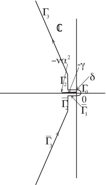
Figure 3: Contour $\Gamma$ for the estimate of the semi-group used in Lemma 13.

2.5.2 Study of the semi-group $e^{\bm{L}_{(\nu)}t}$ in $\mathring{L}_{\eta}^{2}$

The following Lemma, which can be found in [12] chap VII, uses the holomorphy of the semi-group $e^{\bm{L}_{(\nu)}t}:$

Lemma 14.

If there exists $M>0$ such that the following estimate holds

$$\Bigl\|(\mathbb{I}-\varepsilon\bm{L}_{(\nu)}^{(0)})^{-1}\Bigr\|_{\mathcal{L}(\mathring{H}_{\eta}^{1},\mathring{H}_{\eta}^{2})}\leq M\varepsilon^{-1/2},\text{ }\varepsilon\in(0,\delta_{0})\text{, }\delta_{0}>0,$$ (9)

then there exists $C>0$ such that

$$\Bigl\|e^{\bm{L}_{(\nu)}^{(0)}t}\Bigr\|_{\mathcal{L}(\mathring{H}_{\eta}^{1},\mathring{H}_{\eta}^{2})}\leq\frac{C}{t^{1/2}},\text{ }t\in(0,1].$$ (10)

In the Appendix 6.7, we will prove the following Lemma.

Lemma 15.

There exists $M>0$ such that the estimate (9) holds in $\mathcal{L}(\mathring{H}_{\eta}^{1};\mathring{H}_{\eta}^{2})$.

Let us now consider the linear operator $\bm{L}_{(\nu)}=\bm{L}_{(\nu)}^{(0)}+\bm{L}^{(1)}$ acting in $\mathring{L}_{\eta}^{2}$. We have

$$\mathbb{I}-\varepsilon\bm{L}_{(\nu)}=(\mathbb{I}-\varepsilon\bm{L}_{(\nu)}^{(0)})\Bigl(\mathbb{I}-\varepsilon(\mathbb{I}-\varepsilon\bm{L}_{(\nu)}^{(0)})^{-1}\bm{L}^{(1)}\Bigr),$$

and we note that

$$\Bigl\|\varepsilon(\mathbb{I}-\varepsilon\bm{L}_{(\nu)}^{(0)})^{-1}\bm{L}^{(1)}\Bigr\|_{\mathcal{L}(\mathring{H}_{\eta}^{2})}\leq\Bigl\|\varepsilon(\mathbb{I}-\varepsilon\bm{L}_{(\nu)}^{(0)})^{-1}\Bigr\|_{\mathcal{L}(\mathring{H}_{\eta}^{1},\mathring{H}_{\eta}^{2})}\|\bm{L}^{(1)}\|_{\mathcal{L}(\mathring{H}_{\eta}^{2},\mathring{H}_{\eta}^{1})}\leq M\varepsilon^{1/2},$$

hence, for $\varepsilon$ small enough, $M\varepsilon^{1/2}<1/2$ and the operator $\mathbb{I}-\varepsilon(\mathbb{I}-\varepsilon\bm{L}_{(\nu)}^{(0)})^{-1}\bm{L}^{(1)}$ has a bounded (by $2$) inverse in $\mathcal{L}(\mathring{H}_{\eta}^{2}).$ Therefore,

$$\Bigl\|(\mathbb{I}-\varepsilon\bm{L}_{(\nu)})^{-1}\Bigr\|_{\mathcal{L}(\mathring{H}_{\eta}^{1},\mathring{H}_{\eta}^{2})}\leq 2\Bigl\|(\mathbb{I}-\varepsilon\bm{L}_{(\nu)}^{(0)})^{-1}\Bigr\|_{\mathcal{L}(\mathring{H}_{\eta}^{1},\mathring{H}_{\eta}^{2})}\leq\frac{2M}{\varepsilon^{1/2}}.$$

Applying Lemma 14 to $\bm{L}_{(\nu)},$ we have the following Lemma

Lemma 16.

Assume that the eigenvalues $\lambda$ of $\bm{L}_{(\nu)}$ are such that $\Re\lambda<\gamma<0,$ then, for $\widetilde{u}\in\mathring{H}_{\eta}^{2},$ we have

$$\Bigl\|e^{\bm{L}_{(\nu)}t}\widetilde{u}\Bigr\|_{\mathring{H}_{\eta}^{2}}\leq Me^{-\gamma t}\,\|\widetilde{u}\|_{\mathring{H}_{\eta}^{2}},\text{ }t\geq 0.$$

Moreover, we have the estimate

$$\Bigl\|e^{\bm{L}_{(\nu)}t}\widetilde{u}\Bigr\|_{\mathcal{L}(\mathring{H}_{\eta}^{1},\mathring{H}_{\eta}^{2})}\leq M\Bigl(1+\frac{1}{t^{1/2}}\Bigr)e^{-\gamma t}\text{ for }t>0.$$

Proof.

This results from the fact that the set of (isolated) eigenvalues of $\bm{L}_{(\nu)}$ is located as indicated in Lemma 7, Moreover, we have $\Re\lambda<\gamma$ for $\nu>\nu_{0}$, by definition of $\nu_{0}(\alpha)$. The estimate (10), which is valid on $(0,1)$, can then be extended to $(0,\infty)$ using the $\mathring{H}_{\eta}^{2}$ estimate. ∎

2.6 Study of the quadratic term

Let us define the projections $\widetilde{P}$ and $P_{0}$, which separate the 0-Fourier mode from the oscillating part, by: for any $u\in\mathcal{X}_{\eta}$

$$u = \widetilde{P}u+P_{0}u,$$

$$\widetilde{P}u = \widetilde{u}\in\mathring{L}_{\eta}^{2},\text{ }P_{0}u=u_{0}\in\mathring{L}^{\infty}.$$

The above projections naturally work in $\mathcal{Z}_{\eta}$ or $\mathcal{Y}_{\eta}.$ The aim of this section is to show that the quadratic operator

$$\bm{B}(u,v)=-\frac{1}{2}\Pi\Bigl[(u\cdot\nabla)v+(v\cdot\nabla)u\Bigr]$$

is well defined in $\mathcal{Y}_{\eta}$ for $u$ and $v$ in $\mathcal{Z}_{\eta}$.

Lemma 17.

The quadratic operator $\bm{B}$ is bounded from $\mathcal{Z}_{\eta}$ to $\mathcal{Y}_{\eta}:$ there exists $C>0$ such that

$$\|\bm{B}(u,v)\|_{\mathcal{Y}_{\eta}}\leq C\|u\|_{\mathcal{Z}_{\eta}}\|v\|_{\mathcal{Z}_{\eta}}.$$ (11)

Proof.

Let us decompose $u,$ $v$ in $\mathcal{Z}_{\eta}$

$$u=\widetilde{u}+u_{0},\text{ }v=\widetilde{v}+v_{0}$$

then

$$\widetilde{P}B(u,v) = \widetilde{P}B(\widetilde{u},\widetilde{v})+B(\widetilde{u},v_{0})+B(\widetilde{v},u_{0}),$$

$$P_{0}B(u,v) = P_{0}B(\widetilde{u},\widetilde{v}).$$ (12)

Indeed,

$$(u_{0}\cdot\nabla)v_{0}=u_{0}^{y}Dv_{0}=0\text{ }$$

since $u_{0}^{y}=0$ for $u_{0}\in\mathring{L}^{\infty}.$ This implies that $P_{0}B(u_{0},v_{0})=0.$

Now, we observe that $(\widetilde{u}\cdot\nabla)v_{0}$ and $(u_{0}\cdot\nabla)\widetilde{v}$ satisfy

$$\Bigl\|(\widetilde{u}\cdot\nabla)v_{0}\Bigr\|_{L_{\eta}^{2}}^{2}=\sum_{|n|\geq 1}\|\widetilde{u}_{n}^{y}Dv_{0}^{x}\|_{C_{\eta}^{0}}^{2}\leq\|v_{0}\|_{W^{1,\infty}}^{2}\|\widetilde{u}\|_{L_{\eta}^{2}}^{2},$$

$$\Bigl\|(\widetilde{u}\cdot\nabla)v_{0}\Bigr\|_{H_{\eta}^{1}}^{2} = \sum_{|n|\geq 1}n^{2}\|\widetilde{u}_{n}^{y}Dv_{0}^{x}\|_{C_{\eta}^{0}}^{2}+\|D(\widetilde{u}_{n}^{y}Dv_{0}^{x})\|_{C_{\eta}^{0}}^{2}$$

$$\leq \|v_{0}\|_{W^{1,\infty}}^{2}\|\widetilde{u}\|_{H_{\eta}^{1}}^{2}+\|v_{0}\|_{W^{2,\infty}}^{2}\|\widetilde{u}\|_{L_{\eta}^{2}}^{2},$$

and analogously for $(u_{0}\cdot\nabla)\widetilde{v}.$ Hence, as $\Pi$ is bounded from $H_{\eta}^{1}$ to $\mathring{H}_{\eta}^{1},$ we obtain easily

$$\Bigl\|B(\widetilde{u},v_{0})+B(\widetilde{v},u_{0})\Bigr\|_{\mathring{H}_{\eta}^{1}} \leq C\Bigl(\|\widetilde{u}\|_{H_{\eta}^{1}}\|v_{0}\|_{W^{2,\infty}}+\|\widetilde{v}\|_{H_{\eta}^{1}}\|u_{0}\|_{W^{2,\infty}}\Bigr)$$

$$\leq C\|u\|_{\mathcal{Z}_{\eta}}\|v\|_{\mathcal{Z}_{\eta}}.$$

Now, before considering $(\widetilde{u}\cdot\nabla)\widetilde{v}$, let us first consider the product of a scalar function $f$ in $H_{\eta}^{1}$ with a scalar $g$ function in $L_{\eta}^{2},$ both with 0-average. We show that the product $fg$ is in $L_{\eta}^{2}.$ Indeed, the Fourier coefficients satisfy

$$(fg)_{n}=\sum_{p,q=n-p}f_{p}g_{q}$$

and

$$\|(fg)_{n}\|_{C_{\eta}^{0}}\leq\sum_{p\neq 0,q=n-p\neq 0}\frac{1}{p}\|pf_{p}\|_{C_{\eta}^{0}}\|g_{q}\|_{C_{\eta}^{0}},$$

so that

$$\|(fg)_{n}\|_{C_{\eta}^{0}}^{2}\leq\left(\sum_{p^{\prime}\neq 0}\frac{1}{p^{\prime 2}}\right)\sum_{p,q=n-p}\|pf_{p}\|_{C_{\eta}^{0}}^{2}\|g_{q}\|_{C_{\eta}^{0}}^{2}.$$

Hence

$$\|fg\|_{L_{\eta}^{2}}^{2}\leq C\sum_{n,p,q=n-p}\|pf_{p}\|_{C_{\eta}^{0}}^{2}\|g_{q}\|_{C_{\eta}^{0}}^{2}\leq C\|f\|_{H_{\eta}^{1}}^{2}\|g\|_{L_{\eta}^{2}}^{2}.$$

Coming back to $(\widetilde{u}\cdot\nabla)\widetilde{v}$ , with $\widetilde{u}$ and $\widetilde{v}$ in $H_{\eta}^{2},$ we deduce immediately that $\widetilde{P}(\widetilde{u}\cdot\nabla)\widetilde{v}\in H_{\eta}^{1},$ and the bound (11) for $\widetilde{P}B(\widetilde{u},\widetilde{v})$ holds immediately in $\mathring{H}_{\eta}^{1}.$

For the 0-Fourier mode, we have also

$$\|(fg)_{0}\|_{L_{\eta}^{\infty}}^{2}\leq\left(\sum_{p^{\prime}\neq 0}\frac{1}{p^{\prime 2}}\right)\sum_{p}\|pf_{p}\|_{C_{\eta}^{0}}^{2}\|g_{-p}\|_{C_{\eta}^{0}}^{2}\leq C\|f\|_{H_{\eta}^{1}}^{2}\|g\|_{L_{\eta}^{2}}^{2},$$

so that $P_{0}(\widetilde{u}\cdot\nabla)\widetilde{v}$ satisfies easily

$$\|P_{0}(\widetilde{u}\cdot\nabla)\widetilde{v}\|_{W_{\eta}^{1,\infty}}\leq C\|\widetilde{u}\|_{H_{\eta}^{2}}\|\widetilde{v}\|_{H_{\eta}^{2}},$$

and estimate (11) holds. ∎

3 Nonlinear stability of $U$

In this section, we consider the nonlinear evolution problem with an initial data close to the basic flow $U,$ assuming that the spectrum of the linearized operator $\bm{L}_{(\nu)}$ is situated on the left side of the imaginary axis, except the essential spectrum which contains the full negative real line. We prove the nonlinear stability of $U.$

Assume $\xi>0$ and let us define the Banach space $\mathcal{Z}_{\eta,\xi}$ by

$$\mathcal{Z}_{\eta,\xi}=\Bigl\{v=\widetilde{v}+v_{0};\,\widetilde{v}\in C^{0}(\mathbb{R}^{+},\mathring{H}_{\eta}^{2}),\,v_{0}\in C^{0}(\mathbb{R}^{+},\mathring{W}^{2,\infty}),$$

$$|||v|||_{\eta,\xi}=\underset{t\geq 0}{\sup}\Bigl(\|\widetilde{v}(t)e^{\xi t}\|_{\mathring{H}_{\eta}^{2}}+\|(1+t)v_{0}(t)\|_{\mathring{W}^{2,\infty}}\Bigr)<\infty\Bigr\}.$$

Note the exponential weight in time for the non zero Fourier component and the $(1+t)$ weight in time for the zero Fourier component. We now detail the stability part of the Theorem 1 of the introduction.

Theorem 18.

Let us assume $\eta>0$ and assume that the set of eigenvalues $\lambda$ of operator $\bm{L}_{(\nu)}$ satisfies

$$\Re\lambda<-\xi<0,$$

then there exists $\varepsilon>0$ such that for

$$\|\widetilde{P}v(0)\|_{\mathring{H}_{\eta}^{2}}+\|P_{0}v(0)\|_{\mathring{W}_{\eta}^{2}}\leq\varepsilon,$$

there exists a unique solution $v\in\mathcal{Z}_{\eta,\xi}$ of the following differential equation in $\mathcal{X}_{\eta}$

$$\frac{dv}{dt}=\bm{L}_{(\nu)}v+B(v,v),$$ (13)

with $v_{t=0}=v(0)=\widetilde{P}v(0)+P_{0}v(0).$ Moreover there exists $M>0$ such that

$$|||\widetilde{P}v|||_{\eta,\xi} \leq M\|\widetilde{P}v(0)\|_{\mathring{H}_{\eta}^{2}},$$

$$|||P_{0}v|||_{\eta,\xi} \leq M\Bigl(\|P_{0}v(0)\|_{\mathring{W}_{\eta}^{2}}+\|\widetilde{P}v(0)\|_{\mathring{H}_{\eta}^{2}}^{2}\Bigr).$$

Remark 19.

Note that this Theorem implies that

$$\|\widetilde{P}v(t)\|_{\mathring{H}_{\eta}^{2}} \leq Me^{-\xi t}\|\widetilde{P}v(0)\|_{\mathring{H}_{\eta}^{2}},\text{ }t\geq 0,$$

$$\|P_{0}v(t)\|_{\mathring{W}^{2,\infty}} \leq \frac{M}{1+t}\Bigl(\|P_{0}v(0)\|_{\mathring{W}_{\eta}^{2}}+\|\widetilde{P}v(0)\|_{\mathring{H}_{\eta}^{2}}^{2}\Bigr),\text{ }t\geq 0.$$

The slow decrease of the $0$-mode as $t\rightarrow\infty$ is due to the influence of the essential spectrum of $\bm{L}_{(\nu)}$ which contains the full negative real line. Moreover, we may notice that the decay in $y$ at $\infty$ is lost for the $0$-mode for $t>0.$

Proof.

Using (12) and (11) shows that there exists $C>0$ such that we have the estimates

$$\Bigl\|\widetilde{P}B(\widetilde{v},\widetilde{v})+2B(\widetilde{v},v_{0})\Bigr\|_{\mathring{H}_{\eta}^{1}} \leq C\Bigl(\|\widetilde{v}\|_{\mathring{H}_{\eta}^{2}}^{2}+\|\widetilde{v}\|_{\mathring{H}_{\eta}^{2}}\|v_{0}\|_{\mathring{W}^{2,\infty}}\Bigr),$$

$$\|P_{0}B(\widetilde{v},\widetilde{v})\|_{\mathring{W}_{\eta}^{1,\infty}} \leq C\|\widetilde{v}\|_{\mathring{H}_{\eta}^{2}}^{2}.$$

Now (13) becomes

$$\frac{d\widetilde{v}}{dt} = \bm{L}_{(\nu)}\widetilde{v}+\widetilde{P}B(\widetilde{v},\widetilde{v})+2B(\widetilde{v},v_{0}),$$

$$\frac{dv_{0}}{dt} = \bm{L}_{(\nu)}v_{0}+P_{0}B(\widetilde{v},\widetilde{v}),$$

which leads to the following integral formulation for $t\geq 0$

$$\widetilde{v}(t) = e^{\bm{L}_{(\nu)}t}\widetilde{P}v(0)+\int_{0}^{t}e^{\bm{L}_{(\nu)}(t-s)}\Bigl[\widetilde{P}B(\widetilde{v},\widetilde{v})+2B(\widetilde{v},v_{0})\Bigr](s)ds,$$ (14)

$$v_{0}(t) = e^{\bm{L}_{(\nu)}t}P_{0}v(0)+\int_{0}^{t}e^{\bm{L}_{(\nu)}(t-s)}P_{0}B(\widetilde{v},\widetilde{v})(s)ds,$$ (15)

where we look for $\widetilde{v}+v_{0}\in\mathcal{Z}_{\eta,\xi}.$ We can solve the system above by the implicit function theorem with respect to $(\widetilde{v},v_{0})$ in the neighborhood of $0$ for $v(0)=\widetilde{P}v(0)+P_{0}v(0)$ provided

$$\widetilde{P}v(0)\text{ sufficiently small in }\mathring{H}_{\eta}^{2},$$

$$P_{0}v(0)\text{ sufficiently small in }\mathring{W}_{\eta}^{2}.$$

Using the bound of the imaginary parts of eigenvalues which are isolated in the left half complex plane, there exist $\xi_{m}>0$ such that all the eigenvalues $\lambda$ of $\bm{L}_{(\nu)}$ satisfy

$$\sup\Re\lambda=-\xi_{m}<-\xi<0.$$

We choose $\xi_{1}$ such that $-\xi_{m}<-\xi_{1}<-\xi$. Then we have the estimates

$$\|e^{\bm{L}_{(\nu)}t}\|_{\mathcal{L}(\mathring{H}_{\eta}^{2})} \leq Ce^{-\xi_{1}t},\text{ }t\geq 0,$$

$$\|e^{\bm{L}_{(\nu)}t}\|_{\mathcal{L}(\mathring{W}_{\eta}^{2,\infty},\mathring{W}^{2,\infty})} \leq \frac{C}{1+t},\text{ }t\geq 0,$$

$$\|e^{\bm{L}_{(\nu)}(t-s)}\|_{\mathcal{L}(\mathring{H}_{\eta}^{1},\mathring{H}_{\eta}^{2})} \leq C\Bigl[1+\frac{1}{\sqrt{t-s}}\Bigr]e^{-\xi_{1}(t-s)},\text{ }t>s,$$

$$\|e^{\bm{L}_{(\nu)}(t-s)}\|_{\mathcal{L}(\mathring{W}_{\eta}^{1,\infty},\mathring{W}^{2,\infty})} \leq \frac{C}{\sqrt{t-s}(1+\sqrt{t-s})},\text{ }t>s.$$

We note that

$$\|e^{\xi t}e^{\bm{L}_{(\nu)}t}\widetilde{P}v(0)\|_{\mathring{H}_{\eta}^{2}} \leq C\|\widetilde{P}v(0)\|_{\mathring{H}_{\eta}^{2}},$$

$$\|e^{\bm{L}_{(\nu)}t}P_{0}v(0)\|_{\mathring{W}^{2,\infty}} \leq \frac{C}{1+t}\|P_{0}v(0)\|_{\mathring{W}_{\eta}^{2}},$$

that

$$\Bigl\|e^{\xi t}e^{\bm{L}_{(\nu)}(t-s)}\Bigl[\widetilde{P}B(\widetilde{v},\widetilde{v})+2B(\widetilde{v},v_{0})\Bigr](s)\Bigr\|_{\mathring{H}_{\eta}^{2}}$$

$$\leq MC\Bigl(1+\frac{1}{\sqrt{t-s}}\Bigr)e^{-(\xi_{1}-\xi)(t-s)}|||\widetilde{v}|||_{\eta,\xi}|||\widetilde{v}+v_{0}|||_{\eta,\xi},$$

and that

$$\Bigl\|e^{\bm{L}_{(\nu)}(t-s)}P_{0}B(\widetilde{v},\widetilde{v})(s)\Bigr\|_{\mathring{W}^{2,\infty}}\leq\frac{MC}{\sqrt{t-s}(1+\sqrt{t-s})}e^{-2\xi s}|||\widetilde{v}|||_{\eta,\xi}^{2}.$$

Hence the right hand side of (14), and (15) is quadratic and $C^{1}$ in $(\widetilde{v},v_{0})\in\mathcal{Z}_{\eta,\xi}.$ It results by the implicit function theorem, that, provided $(\widetilde{P}v(0),P_{0}v(0))$ small enough in $\mathring{H}_{\eta}^{2}\oplus\mathring{W}_{\eta}^{2},$ there exists a unique solution $(\widetilde{v},v_{0})\in\mathcal{Z}_{\eta,\xi}$ in a neighborhood of $0.$ Moreover, directly from the system (14), (15), we have the estimate

$$\|e^{\xi t}\widetilde{v}(t)\|_{\mathring{H}_{\eta}^{2}}\leq C\|\widetilde{P}v(0)\|_{\mathring{H}_{\eta}^{2}}+MC\int_{0}^{t} (1+\frac{1}{(t-s)^{1/2}})$$

$$\times e^{-(\xi_{1}-\xi)(t-s)}|||\widetilde{v}|||_{\eta,\xi}|||\widetilde{v}+v_{0}|||_{\eta,\xi}ds,$$

hence

$$|||\widetilde{v}|||_{\eta,\xi}\leq C\|\widetilde{P}v(0)\|_{\mathring{H}_{\eta}^{2}}+K|||\widetilde{v}|||_{\eta,\xi}|||\widetilde{v}+v_{0}|||_{\eta,\xi},$$

using

$$\int_{0}^{t}\Bigl[1+\frac{1}{(t-s)^{1/2}}\Bigr]e^{-\delta(t-s)}ds\leq C_{1}(\delta)\text{ for }\delta>0.$$

In the same way, we obtain

$$|||v_{0}|||_{\eta,\xi}\leq C\|P_{0}v(0)\|_{\mathring{W}_{\eta}^{2,\infty}}+K|||\widetilde{v}|||_{\eta,\xi}^{2},$$

using

$$\int_{0}^{t}\frac{1}{\sqrt{t-s})(1+\sqrt{t-s})}e^{-\delta s}ds\leq\frac{C_{2}(\delta)}{1+t},\text{ for }\delta>0.$$

Hence,

$$|||\widetilde{v}|||_{\eta,\xi}\leq C\|\widetilde{P}v(0)\|_{\mathring{H}_{\eta}^{2}}+CK\|P_{0}v(0)\|_{\mathring{W}_{\eta}^{2,\infty}}|||\widetilde{v}|||_{\eta,\xi}+K|||\widetilde{v}|||_{\eta,\xi}^{2}+K^{2}|||\widetilde{v}|||_{\eta,\xi}^{3},$$

so that for $v(0)$ such that

$$CK\|P_{0}v(0)\|_{\mathring{W}_{\eta}^{2,\infty}}+2CK\|\widetilde{P}v(0)\|_{\mathring{H}_{\eta}^{2}}+4C^{2}K^{2}\|\widetilde{P}v(0)\|_{\mathring{H}_{\eta}^{2}}^{2}<\frac{1}{2},$$

we obtain

$$|||\widetilde{v}|||_{\eta,\xi} \leq 2C\|\widetilde{P}v(0)\|_{\mathring{H}_{\eta}^{2}},$$

$$|||v_{0}|||_{\eta,\xi} \leq C\|P_{0}v(0)\|_{\mathring{W}_{\eta}^{2,\infty}}+4C^{2}K\|\widetilde{P}v(0)\|_{\mathring{H}_{\eta}^{2}}^{2}$$

which ends the proof of the nonlinear asymptotic stability. ∎

4 Study of the bifurcation

4.1 Setup

Let us define

$$s=\omega_{0}t$$

such that the time-periodic solution which we are looking for is now $2\pi$ periodic in $s$. The wave number $\omega_{0}$ is an unknown of the bifurcation, which must be determined.

Let us define the bifurcation parameter $\mu$ as

$$\mu=\nu-\nu_{0}$$

By assumption, ${\bf L}:={\bf L}_{(\nu_{0})}$ has two purely imaginary simple eigenvalues $\pm i\omega_{0}$, associated to eigenvectors of the form

$$\zeta=e^{i\alpha x}\hat{v}(y),\quad\overline{\zeta}=e^{-i\alpha x}\overline{\hat{v}(y)}$$ (16)

and no other eigenvalues of non negative real part.

In what follows, we need to invert the linear system

$$\omega_{0}{dv\over ds}-{\bf L}\,v=f$$

in a space of vector functions which are $2\pi$ periodic in $s$ and $2\pi/\alpha$ periodic in $x$. We expand $f$ and $v$ in Fourier series in time and space, $k$ being the Fourier wave number in time and $n$ the Fourier wave number in space. This leads to the sequence of equations

$$ik\omega_{0}v_{k,n}-{\bf L}_{n}v_{k,n}=f_{k,n}$$

where $(k,n)\in\mathbb{Z}^{2}$, and where the linear operator ${\bf L}_{n}$ is defined in a space of vector functions of $y$ by

$${\bf L}_{n}v_{n} =\nu_{0}(D^{2}-n^{2}\alpha^{2})v_{n}+\Bigl(\begin{array}[]{c}i\alpha n\cr D\cr\end{array}\Bigr)q_{n}-in\alpha Uv_{n}-\Bigl(\begin{array}[]{c}v_{n}^{y}U^{\prime}\cr 0\cr\end{array}\Bigr),$$

$$0 =in\alpha v_{n}^{x}+Dv_{n}^{y},$$

where $q_{n}$ is the related component of the pressure. We know by assumption that

• ${\bf L}_{n}-ik\omega_{0}$ is invertible for $n\neq 0$ and $k\neq\pm 1$,

• for $n=1$, ${\bf L}_{n}-i\omega_{0}$ has a 1-dim kernel spanned by $\zeta$,

• for $n=-1$, ${\bf L}_{n}+i\omega_{0}$ has a 1-dim kernel spanned by $\bar{\zeta}$,

• for $n\neq\pm 1$, ${\bf L}_{n}\mp i\omega_{0}$ is invertible,

• for $k\neq 0$, ${\bf L}_{0}-ik\omega_{0}$ is invertible.

It remains to study the invertibility of ${\bf L}_{0}$.

4.2 Study of the inverse of ${\bf L}_{0}$

Lemma 20.

If $f_{0,0}\in L^{\infty}_{\eta}$, then the equation

$${\bf L}_{0}v_{0,0}=\Bigl(\begin{array}[]{c}f_{0,0}\cr 0\cr\end{array}\Bigr)$$ (17)

has a unique solution such that $v_{0,0}^{x}$ is bounded. Moreover,

$$\|v_{0,0}\|_{W^{2,\infty}}\leq C_{\eta}\|f_{0,0}\|_{L^{\infty}_{\eta}}$$

for some positive constant $C_{\eta}$.

Proof.

The equation (17) leads to

$$\nu_{0}D^{2}v_{0,0}=f_{0,0}.$$

Taking care of the boundary condition $v_{0,0}^{x}=0$ at $y=0$ and its boundedness at infinity, we find

$$Dv_{0,0}^{x} ={1\over\nu_{0}}\Bigl[-\int_{y}^{\infty}f_{0,0}(s)\,ds+A\Bigr],$$

$$v_{0,0}^{x} ={1\over\nu_{0}}\int_{0}^{y}d\tau\Bigl[-\int_{\tau}^{\infty}f_{0,0}(s)\,ds+A\Bigr]$$

for some constant $A$ to be determined so that $v_{0,0}^{x}$ is bounded and $Dv_{0,0}^{x}$ tends exponentially to $0$ at infinity. This leads to $A=0$ and to

$$v_{0,0}^{x}(y)=-{1\over\nu_{0}}\int_{0}^{y}d\tau\int_{\tau}^{\infty}f_{0,0}(s)\,ds,$$

and, by Fubini’s theorem,

$$v_{0,0}^{x}(y)=-{1\over\nu_{0}}\Bigl[\int_{0}^{y}sf_{0,0}(s)\,ds+y\int_{y}^{\infty}f_{0,0}(s)\,ds\Bigr],$$

which ends the proof of the Lemma. ∎

We note that

$$\lim_{y\to+\infty}v_{0,0}^{x}(y)=-{1\over\nu_{0}}\int_{0}^{+\infty}sf_{0,0}(s)\,ds,$$

which in general does not vanish. Thus, in general, $v_{0,0}^{x}$ does not go to $0$ at infinity, but $Dv_{0,0}^{x}$ and $D^{2}v_{0,0}^{x}$ decay exponentially fast at infinity. However $v_{0,0}$ only appears in the operator $(v\cdot\nabla)v$, and thus only in terms of the form $(v_{0,0}\cdot\nabla)v$ and $(v\cdot\nabla)v_{0,0}$ where $v$ will be exponentially decaying.

4.3 The eigenvectors $\zeta$ and $\zeta^{\star}$

We look for $\zeta=e^{i\alpha x}\hat{v}(y)\in\mathcal{Z}_{\eta}$ where $\alpha\neq 0$ and $\hat{v}=(\hat{v}^{x},\hat{v}^{y})\in C^{2}_{\eta}$ satisfy

$$i\omega_{0}\hat{v} =\nu_{0}(D^{2}-\alpha^{2})\hat{v}+\Bigl(\begin{array}[]{c}i\alpha\cr D\cr\end{array}\Bigr)\hat{q}-i\alpha U\hat{v}-\Bigl(\begin{array}[]{c}\hat{v}^{y}U^{\prime}\cr 0\cr\end{array}\Bigr),$$

$$0 =i\alpha\hat{v}^{x}+D\hat{v}^{y}$$

with $\hat{v}^{x}=\hat{v}^{y}=0$ for $y=0$. This leads to $\hat{v}^{y}\in C^{4}_{\eta}$ and

$$\Bigl[i\omega_{0}-\nu_{0}(D^{2}-\alpha^{2})-i\alpha U\Bigr](D^{2}-\alpha^{2})\hat{v}^{y}+i\alpha U^{\prime\prime}\hat{v}^{y}=0$$ (18)

with $\hat{v}^{y}=D\hat{v}^{y}=0$ for $y=0$, which is the Orr-Sommerfeld equation.

By assumption, (18) has a non trivial smooth solution $\hat{v}^{y}(y)$, satisfying the boundary conditions, unique up to a multiplicative constant. Moreover, there exist $c_{1}>0$ and $\eta>0$ such that

$$|\hat{v}^{y}(y)|+|D\hat{v}^{y}(y)|\leq c_{1}e^{-\eta y}$$

for $0\leq y<+\infty$. It results that there exists $c>0$ and $\eta>0$ such that

$$|\hat{v}(y)|+|D\hat{v}(y)|\leq ce^{-\eta y}$$

for $0\leq y<+\infty$ (see [9]).

4.4 Pseudo-inverse of $\omega_{0}d/ds-{\bf L}$

The aim of this section is to construct a pseudo inverse to the linear operator

$$\mathcal{L}=\omega_{0}{d\over ds}-{\bf L}$$

in a space of $2\pi$ periodic vector functions (periodic in time and space).

Let us define $\zeta^{*}$, the eigenvector of ${\bf L}^{\star}$ for the eigenvalue $-i\omega_{0}$, such that $\langle\zeta,\zeta^{\star}\rangle=1$ (see [13]). Let $\mathbb{T}_{1}=\mathbb{R}/2\pi\mathbb{Z}$. Let $\mathcal{H}$ be a subspace of $L^{2}(\mathbb{T}_{1},\mathcal{X}_{\eta})$ such that, for every $v\in\mathcal{H}$,

$$\langle v,e^{is}\zeta^{\star}\rangle_{\mathcal{H}}=\langle v,e^{-is}\overline{\zeta}^{\star}\rangle_{\mathcal{H}}=0$$

and such that $v_{00}=0$. Let us define

$$H^{\sharp}=H^{1}(\mathbb{T}_{1},\mathcal{X}_{\eta})\cap L^{2}(\mathbb{T}_{1},\mathcal{Z}_{\eta}),$$

together with its norm

$$\|v\|_{H^{\sharp}}^{2}=\|\partial_{s}v\|_{L^{2}(\mathbb{T}_{1},\mathcal{X}_{\eta})}^{2}+\|v\|_{L^{2}(\mathbb{T}_{1},\mathcal{Z}_{\eta})}^{2}.$$

Lemma 21.

For $f\in\mathcal{H}$, there exists a unique $v\in H^{\sharp}\cap\mathcal{H}$ such that

$$\Bigl(\omega_{0}{d\over ds}-{\bf L}\Bigr)v=f.$$

This defines a pseudo-inverse $\mathcal{L}^{-1}$ to ${\cal L}$ which satisfies

$$\|v\|_{H^{\sharp}}\leq\|f\|_{\mathcal{H}}.$$

Proof.

As $f\in\mathcal{H}$, $f$ is of the form

$$f(x,y,s)=\sum_{(n,k)\in\mathbb{Z}^{2}}f_{k,n}(y)e^{i(ks+n\alpha x)}$$

with

$$\Bigl\langle f_{1,1}e^{i\alpha x},\zeta^{\star}\Bigr\rangle=\Bigl\langle f_{-1,-1}e^{-i\alpha x},\overline{\zeta^{\star}}\Bigr\rangle=0,\quad f_{0,0}=0.$$

Similarly, we look for $v\in\mathcal{H}$, namely for a function $v$ of the form

$$v(x,y,s)=\sum_{(n,k)\in\mathbb{Z}^{2}}v_{k,n}(y)e^{i(ks+n\alpha x)}$$

with

$$\Big\langle v_{1,1}e^{i\alpha x},\zeta^{\star}\Big\rangle=\Big\langle v_{-1,-1}e^{-i\alpha x},\overline{\zeta^{\star}}\Big\rangle=0,\quad v_{00}=0.$$

This leads to

$$\Bigl(ik\omega_{0}-{\bf L}_{n}\Bigr)v_{k,n}=f_{k,n}$$ (19)

for $(k,n)\neq\pm(1,1)$ and $(k,n)\neq(0,0)$.

Using Lemma 10, we know that there exist $k_{0}$ and $c$ such that if $|k|>k_{0}$ is large enough, the equation (19) has a unique solution such that

$$\|D^{2}v_{k,n}\|_{C^{0}_{\eta}}+|n|\,\|Dv_{k,n}\|_{C^{0}_{\eta}}+(1+n^{2})\|v_{k,n}\|_{C^{0}_{\eta}}\leq\|f_{k,n}\|_{C^{0}_{\eta}},$$ (20)

and

$$\|v_{k,n}\|_{C^{0}_{\eta}}\leq{c\over|k|}\|f_{k,n}\|_{C^{0}_{\eta}}$$

provided $(k,n)\neq\pm(1,1),(0,0)$.

For $n\neq\pm 1$, $n\neq 0$ and $|k|\leq k_{0}$, ${\bf L}_{n}$ is invertible by assumption in section $2.1$, thus (20) is still valid (up to the change of the factor $c>0$). For $n=\pm 1$, (20) is also valid since $f_{k,n}$ is orthogonal to $\zeta^{\star}$ and $\overline{\zeta^{\star}}$, and thus in the range of $ik\omega_{0}-{\bf L}_{n}$. For $n=0$, as $f_{0,0}=0$, $v_{0,0}=0$, and we just have to consider the case $k\neq 0$, where $ik\omega_{0}-{\bf L}_{0}$ is invertible by Lemma 10, thus (20) is still valid.

Combining all these estimates, we get that the pseudo inverse of $\mathcal{L}$ is bounded from ${\cal H}$ to $H^{\sharp}$. ∎

4.5 Bifurcation of a time periodic solution

We are looking for a solution $v$, which is $2\pi$ periodic in $s$, $2\pi/\alpha$ periodic in $x$, of the non linear equation

$$\Bigl[\omega{d\over ds}-{\bf L}\Bigr]v=\mu{\bf L}^{\prime}v+B(v,v)$$ (21)

where

$${\bf L}^{\prime}v=\Pi\Delta v,$$

$$B(v,v)=-\Pi(v\cdot\nabla)v.$$

Let

$$H^{\sharp\sharp}=H^{2}(\mathbb{T}_{1},\mathcal{X}_{\eta})\cap H^{1}(\mathbb{T}_{1},\mathcal{Z}_{\eta}).$$

We decompose $v\in H^{\sharp\sharp}$ as

$$v=\underline{v}+w,$$

$$\underline{v}=Ae^{is}\zeta+\overline{A}e^{-is}\bar{\zeta}+v_{0,0},$$

$$\langle w_{1,1}e^{i\alpha x},\zeta^{\star}\rangle=\langle w_{-1,-1}e^{-i\alpha x},\overline{\zeta^{\star}}\rangle=0,$$

$$w_{0,0}=0,$$

and define the projection $\mathfrak{P}_{0}$ by

$$w=\mathfrak{P}_{0}v.$$

The projection $\mathfrak{P}_{0}$ is bounded in $H^{1}(\mathbb{T}_{1},{\cal X}_{\eta})$ and in $H^{\sharp\sharp}$ and commutes with the linear operator $(\omega\partial_{s}-{\bf L})$. Later we will use the fact that our system is invariant under two different $SO(2)$ symmetries, an hence commutes with the operator $T_{a}$ representing the translation in time $s\to s+a$, and the operator $\tau_{\beta}$ representing the translation in space $x\to x+\beta$.

Let

$$\xi=x+{s\over\alpha}.$$

We now prove the following bifurcation theorem, which precises Theorem 1 and gives an expansion of the bifurcation parameter $\mu$, of the time frequency $\omega$ and of the time and space periodic solution near the bifurcation point in terms of the amplitude $\varepsilon$.

Theorem 22.

For $\mu$ in a right or left neighborhood of $0$, there exists a bifurcated time-periodic solution of (21) which is a traveling wave function $\widehat{V}_{\varepsilon}(\xi,y)$, of the form

$$\widehat{V}_{\varepsilon}=\varepsilon V_{1}+\varepsilon^{2}V_{2}+\mathcal{O}(\varepsilon^{3})\in\mathcal{Z}_{\eta},$$

with

$$V_{1} = (e^{i\alpha\xi}\widehat{\zeta}+e^{-i\alpha\xi}\overline{\widehat{\zeta}})\text{ }\in\mathring{H}_{\eta}^{2},$$

$$V_{2} = \widehat{w}_{2,2}e^{2i\alpha\xi}+\overline{\widehat{w}_{2,2}}e^{-2i\alpha\xi}+v_{2,0},$$

$$\mu(\varepsilon) = \varepsilon^{2}\mu_{2}+\mathcal{O}(\varepsilon^{4}),$$

$$\omega(\varepsilon) = \omega_{0}+\varepsilon^{2}\omega_{2}+\mathcal{O}(\varepsilon^{4}),$$

Moreover, we have

$$\mu_{2}\Bigl\langle(D^{2}-\alpha^{2})\widehat{\zeta},\widehat{\zeta}^{\ast}\Bigr\rangle-i\omega_{2} = c-b,\text{ }\Re\Bigl\langle(D^{2}-\alpha^{2})\widehat{\zeta},\widehat{\zeta}^{\ast}\Bigr\rangle>0,$$

$$\widehat{w}_{2,2}e^{2i\alpha\xi} = (2i\omega_{0}-\bm{L}^{(0)})^{-1}B(e^{i\alpha\xi}\widehat{\zeta},e^{i\alpha\xi}\widehat{\zeta})\in\mathring{H}_{\eta}^{2},$$

$$v_{2,0} = -2L_{0}^{-1}B(e^{i\alpha\xi}\widehat{\zeta},e^{-i\alpha\xi}\overline{\widehat{\zeta}})\in\mathring{W}^{2,\infty},$$

$$c = -\Bigl\langle 2B(e^{i\alpha\xi}\widehat{\zeta},v_{2,0}),e^{i\alpha\xi}\widehat{\zeta}^{\ast}\Bigr\rangle,$$

$$b = \Bigl\langle 2B(e^{-i\alpha\xi}\overline{\widehat{\zeta}},e^{2i\alpha\xi}\widehat{w}_{2,2}),e^{i\alpha\xi}\widehat{\zeta}^{\ast}\Bigr\rangle,$$

We note that the bifurcation is supercritical if $\mu_{2}>0$, i.e. $\Re(c-b)>0$, where

$$c-b=\Bigl\langle 4B\Bigl(\zeta,{\bf L}_{0}^{-1}B(\zeta,\overline{\zeta})-2B(\bar{\zeta},(2i\omega_{0}-L)^{-1}B(\zeta,\zeta)\Bigr),\zeta^{\star}\Bigr\rangle.$$

Proof.

We use an adapted Lyapunov-Schmidt method (variant of the implicit function theorem). Using the decomposition $v=\underline{v}+w$, the system becomes

$$\Bigl(\omega_{0}{d\over ds}-{\bf L}\Bigr)w-{\bf L}_{0}v_{0,0}=\mu{\bf L}^{\prime}v-(\omega-\omega_{0}){dv\over ds}+B(v,v),$$

where we look for $v$ such that $w\in\mathfrak{P}_{0}H^{\sharp\sharp}$, $A\in\mathbb{C}$, $v_{0,0}\in W^{2,\infty}$ when $(\mu,\omega-\omega_{0})$ is close to $0$ in $\mathbb{R}^{2}$. After decomposition, this becomes

$$\Bigl(\omega_{0}{d\over ds}-{\bf L}\Bigr)w =\mu\mathfrak{P}_{0}{\bf L}^{\prime}(\underline{v}+w)-(\omega-\omega_{0}){dw\over ds}+\mathfrak{P}_{0}B(\underline{v}+w,\underline{v}+w),$$ (22)

$$\Big\langle\mu{\bf L}^{\prime}(\underline{v}+w)-(\omega-\omega_{0}){d\underline{v}\over ds}+B(\underline{v}+w,\underline{v}+w),\zeta^{\star}e^{is}\Big\rangle=0,$$ (23)

$${\bf L}_{0}v_{0,0}+\mu{\bf L}^{\prime}v_{0,0}+\Big[B(\underline{v}+w,\underline{v}+w)\Bigr]_{0,0}=0,$$ (24)

where we look for solutions $(w,A,v_{0,0})$ in a neighborhood of $0$ in

$$\mathfrak{P}_{0}H^{\sharp\sharp}\times\mathbb{C}\times W^{2,\infty}.$$

We first solve (22) with respect to $w\in\mathfrak{P}_{0}H^{\sharp\sharp}$ in function of $\underline{v}$, $\omega-\omega_{0}$, $v_{0,0}$ and $\mu$ in a neighborhood of $0$. Moreover, the choice of our spaces (see (20)) implies that

$${dw\over ds},\mathfrak{P}_{0}B(v,v)\in H^{1}(\mathbb{T}_{1},{\cal X}_{\eta}),$$

which allows to apply the implicit function theorem with respect to $w$. The principal part which is independent of $w$ in the right hand side of (22), is

$$\mu{\bf L}^{\prime}\underline{v}+\mathfrak{P}_{0}B(\underline{v},\underline{v})$$

so we find

$$w=W(A,\overline{A},\omega-\omega_{0},\mu,v_{0,0})\in\mathfrak{P}_{0}H^{\sharp\sharp},$$

with

$$W(A,\overline{A},\omega-\omega_{0},\mu,v_{0,0}) =\Bigl(\omega_{0}{d\over ds}-{\bf L}\Bigr)^{-1}\Bigl[\mu\mathfrak{P}_{0}{\bf L}^{\prime}\underline{v}+\mathfrak{P}_{0}B(\underline{v},\underline{v})\Bigr]$$

$$\quad+O\Bigl(\|\underline{v}\|^{3}+\Bigl[|\mu|+|\omega-\omega_{0}|\Bigr]\|\underline{v}\|^{2}+|\mu|\,|\omega-\omega_{0}|\,\|\underline{v}\|\Bigr).$$

We note that for $A=0$, id est for $\underline{v}=v_{0,0}$, we have

$$W(0,0,\omega-\omega_{0},\mu,v_{0,0})=0.$$

Using now $T_{a}$, we have

$$T_{a}(A\zeta e^{is})=Ae^{ia}\zeta e^{is},\qquad T_{a}\underline{v}(s)=\underline{v}(s+a),$$

hence, the commuting property leads to

$$T_{a}W(A,\overline{A},\omega-\omega_{0},\mu,v_{0,0})=W(e^{ia}A,e^{-ia}\overline{A},\omega-\omega_{0},\mu,v_{0,0}).$$

Moreover, we note that, using $\tau_{-a/\alpha}$

$$T_{a}\tau_{-a/\alpha}=Id,\text{ for any }a\in\mathbb{R}$$ (25)

on the $\underline{v}$ part.

Replacing $w$ by $W$ in equations (23) and (24), we obtain an infinite dimensional system

$$F(A,\overline{A},\omega-\omega_{0},\mu,v_{0,0}) =0,$$

$${\bf L}_{0}v_{0,0}+\mu{\bf L}^{\prime}v_{0,0}+[B(\underline{v}+W,\underline{v}+W)]_{0,0} =0.$$

We note that, applying $T_{a}$ for any $a\in\mathbb{R}$,

$$F(e^{ia}A,e^{-ia}\overline{A},\omega-\omega_{0},\mu,v_{0,0})=e^{ia}F(A,\overline{A},\omega-\omega_{0},\mu,v_{0,0}),$$

so that $A$ is in factor in $F$, which only depends on $|A|^{2}$. Moreover

$$\Big\langle\mu{\bf L}^{\prime}(\underline{v}+W),\zeta^{\star}e^{is}\Big\rangle=A\mu\langle\Delta\zeta,\zeta^{\star}\rangle+O(|\mu|\,\|W\|),$$

$$\Big\langle(\omega-\omega_{0}){d\underline{v}\over ds},\zeta^{\star}e^{is}\Big\rangle=iA(\omega-\omega_{0}),$$

$$\Big\langle B(\underline{v},\underline{v}),\zeta^{\star}e^{is}\Big\rangle=2A\Big\langle B(\zeta,v_{0,0}),\zeta^{\star}\Big\rangle,$$

hence, it is clear that $F$ is of the form

$$0 =A\mu\langle\Delta\zeta,\zeta^{\star}\rangle-iA(\omega-\omega_{0})+bA|A|^{2}+2A\langle B(\zeta,v_{0,0}),\zeta^{\star}\rangle$$ (26)

$$\quad+O\Bigl(|A|\,|\mu|^{2}+|\mu|\,|A|^{2}+|\mu|\,|A|\,|v_{0,0}|+|A|\,|v_{0,0}|^{2}+|A|^{4}\Bigr)$$ (27)

where

$$b=2\Big\langle B\Big(\overline{\zeta},(2i\omega_{0}-L)^{-1}B(\zeta,\zeta)\Big),\zeta^{\star}\Big\rangle.$$ (28)

Finally, looking for $A\neq 0$ leads to

$$0 =\mu\langle\Delta\zeta,\zeta^{\star}\rangle-i(\omega-\omega_{0})+b|A|^{2}+2\langle B(\zeta,v_{0,0}),\zeta^{\star}\rangle$$ (29)

$$\quad+O\Bigl(|\mu|^{2}+(|\mu|+|\omega-\omega_{0}|)|A|^{2}+|A|^{4}\Bigr).$$ (30)

Let us notice that

$$\langle{\bf L}^{\prime}\zeta,\zeta^{\star}\rangle=\langle\Delta\zeta,\zeta^{\star}\rangle=\partial_{\nu}\lambda(\alpha,\nu_{0}(\alpha)).$$

The $(0,0)$ mode equation (24) has a very specific form. Indeed, let $P_{0}$ be the projection giving the 0-Fourier mode. We observe that

$$B(P_{0}v,P_{0}v)=0,\text{ for any }v\in W^{2,\infty},$$

hence the term $B(\underline{v}+W,\underline{v}+W)$ decays like $e^{-\eta y}$. It results that $[B(\underline{v}+W,\underline{v}+W)]_{0,0}\in L_{\eta}^{\infty}$. Moreover we observe that

$${\bf L}_{0,0}+\mu{\bf L}^{\prime}=(1+\frac{\mu}{\nu_{0}}){\bf L}_{0,0},$$

hence, using Lemma 20, (24) may be written in $W^{2,\infty}$ as

$$(1+\frac{\mu}{\nu_{0}})v_{0,0}+{\bf L}_{0,0}^{-1}[B(\underline{v}+W,\underline{v}+W)]_{0,0}=0,$$

which can be solved in $v_{0,0}\in W^{2,\infty}$ by the implicit function theorem, noticing that $A$ only occurs through $|A|^{2}$. The principal part which is independent of $v_{0,0}$ in (24) is

$$\Bigl[B\Bigl(Ae^{is}\zeta+\bar{A}e^{-is}\bar{\zeta},Ae^{is}\zeta+\bar{A}e^{-is}\bar{\zeta}\Bigr)\Bigr]_{0,0}=2|A|^{2}B(\zeta,\bar{\zeta})\in C^{0}_{\eta}.$$

This leads to

$$v_{0,0}=-2|A|^{2}{\bf L}_{0,0}^{-1}B(\zeta,\overline{\zeta})+O\Bigl(|\mu|\,|A|^{2}+|A|^{4}\Bigr).$$

Replacing $v_{0,0}$ by its expression in (29) leads to a two dimensional real system, which can be solved by the implicit function theorem, with respect to $\mu$ and $\omega-\omega_{0}$. The equivariance of the system under the groups $T_{a}$ and $\tau_{\beta}$ implies that (25) also holds on $W$. Thus we obtain a traveling wave, with a function depending on $(s,x)$ through $x+s/\alpha$. Defining

$$c=4\Big\langle B(\zeta,L_{0,0}^{-1}B(\zeta,\overline{\zeta})),\zeta^{\star}\Big\rangle,$$

we finally obtain the bifurcating solution, parametrized by $A$ (defined up to a phase shift)

$$\mu ={\Re(c-b)\over\Re\langle\Delta\zeta,\zeta^{\star}\rangle}|A|^{2}+O(|A|^{4})$$

$$\omega-\omega_{0} =\Bigl(\Im(b-c)+{\Re(c-b)\Im\langle\Delta\zeta,\zeta^{\star}\rangle\over\Re\langle\Delta\zeta,\zeta^{\star}\rangle}\Bigr)|A|^{2}+O(|A|^{4}),$$

$$v_{0,0} =-2|A|^{2}L_{0,0}^{-1}B(\zeta,\overline{\zeta})+O(|A|^{4})\in W^{2,\infty},$$

$$w =A^{2}e^{2is}(2i\omega_{0}-L)^{-1}B(\zeta,\zeta)+c.c.+O(|A|^{3})\in\mathfrak{P}_{0}H^{\sharp\sharp},$$

$$v =Ae^{is}\zeta+\overline{A}e^{-is}\overline{\zeta}+v_{0,0}+w.$$

The theorem is proved as soon as we replace $|A|$ by $\varepsilon$. ∎

We note that the phase of $A$ is arbitrary, which corresponds to an arbitrary shift parallel to the $x$ axis , or to a shift in time. Moreover, by assumption,

$$\Re\langle\Delta\zeta,\zeta^{\star}\rangle>0.$$

Then, the supercriticality or subcriticality of the bifurcation depends on the sign of $\Re(c-b)$ which needs to be computed.

5 Nonlinear stability of the bifurcating traveling wave

In all what follows the bracket $\langle\cdot,\cdot\rangle$ is understood as the duality product between $\mathcal{X}_{\eta}=\mathring{L}_{\eta}^{2}\oplus\mathring{L}^{\infty}$ and $\mathcal{X}_{\eta}^{\ast}=(\mathring{L}_{\eta}^{2})^{\ast}\oplus\mathring{L}^{1}$.

5.1 Study of the linearized operator

We proved that the bifurcating periodic solution is in fact a travelling wave, function of $(\alpha x+\omega t,y).$ It is then natural to change coordinates and to replace $x$ by

$$\xi=x+\frac{\omega t}{\alpha}.$$

With these coordinates, we define

$$\widehat{v}(\xi,y,t)=v(x,y,t),$$

so that the Navier-Stokes system becomes

$$\frac{d\widehat{v}}{dt}=\bm{L}_{\nu,\omega}\widehat{v}+B(\widehat{v},\widehat{v}),\quad\nabla\cdot\widehat{v}=0,$$ (31)

with

$$\bm{L}_{\nu,\omega}\widehat{v}=\bm{L}_{(\nu)}\widehat{v}-\frac{\omega}{\alpha}\frac{\partial\widehat{v}}{\partial\xi}=\bm{L}^{(0)}\widehat{v}+\mu\bm{L}^{\prime}\widehat{v}-\frac{\omega}{\alpha}\frac{\partial\widehat{v}}{\partial\xi},$$

where

$$\bm{L}^{(0)}=\bm{L}_{(\nu_{0})}^{(0)}+\bm{L}^{(1)}.$$

The linear operator $\bm{L}_{\nu,\omega}$ is acting in $\mathcal{X}_{\eta}$, with domain $\mathcal{Z}_{\eta}.$ In the following we need to localize the essential spectrum of the linear operator

$$\bm{L}_{(\nu)}^{(0)}+\bm{L}^{(0,1)}-\frac{\omega}{\alpha}\frac{\partial}{\partial\xi}=\nu\Pi\Delta-\frac{\omega+\alpha U_{+}}{\alpha}\frac{\partial}{\partial\xi}$$

in $\bm{\mathring{L}}_{\eta}^{2}.$ This is described in the following Lemma.

Lemma 23.

There exists $\eta>0$ small enough, such that for any $\lambda$ in the spectrum of

$$\nu\Pi\Delta-\frac{\omega+\alpha U_{+}}{\alpha}\frac{\partial}{\partial\xi}$$

acting in $\bm{\mathring{L}}_{\eta}^{2}$, we have $\lambda\in\Sigma_{U_{+},\omega}$ where (see Figure 4)

$$\Sigma_{U_{+},\omega}= \Bigl\{\Re\lambda\leq-\nu(\alpha^{2}-\eta^{2})\Bigr\}$$

$$\cap \Bigl\{\,\Bigl\{2\pi/3\leq\arg|(\lambda_{0}+\nu\alpha^{2})|\leq\pi\Bigr\}\cup\Bigl\{\Re\lambda\leq-\frac{\nu\alpha^{2}}{(\omega+\alpha U_{+})^{2}+4\nu^{2}\alpha^{2}\eta^{2}}(\Im\lambda)^{2}+\eta^{2}\nu\Bigr\}\,\Bigr\}.$$

For $\lambda$ outside of this region $\Sigma_{U+,\omega}$, where

$$0\leq|\arg(\lambda_{0}+\nu\alpha^{2})|\leq\frac{2\pi}{3}-\delta$$

with $0<\delta<\pi/6$, and where we add some small $\delta_{1}$ to $U_{+}$, there exists $C>0$ such that

$$\Bigl\|\Bigl(\nu\Pi\Delta-\frac{\omega+\alpha U_{+}}{\alpha}\frac{\partial}{\partial\xi}-\lambda\mathbb{I}\Bigr)^{-1}\Bigr\|_{\mathcal{L}(\bm{\mathring{L}}_{\eta}^{2})}\leq\frac{C}{|\lambda+\nu\alpha^{2}|}.$$

The proof of this Lemma is identical to the proof of Lemma 9 for the essential spectrum, up to the change of $U_{+}$ in $U_{+}+\omega/\alpha$. This enlarges the parabolic region.

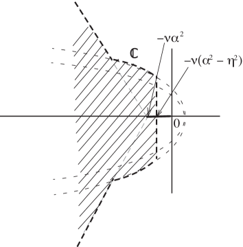
Figure 4: Hatched region $\Sigma_{U_{+},\omega}$ and negative real line containing the spectrum of $\nu\Pi\Delta-(U_{+}+\frac{\omega}{\alpha})\frac{\partial}{\partial\xi}$ and the essential spectrum of $\bm{L}_{\nu,\omega}$.

We know that there is a bifurcating steady solution of (31) which is

$$\widehat{V}_{\varepsilon}(\xi,y)\overset{def}{=}V_{\varepsilon}(x,y,t),\text{ }\omega=\omega(\varepsilon),\mu=\mu(\varepsilon),$$

as described in Theorem 22.

Now we introduce $\phi_{0}^{\ast},\phi_{1}^{\ast}\in(\mathring{L}_{\eta}^{2})^{\ast}$ defined by

$$\phi_{0}^{\ast} = \frac{i}{2}(e^{i\alpha\xi}\widehat{\zeta^{\ast}}-e^{-i\alpha\xi}\overline{\widehat{\zeta^{\ast}}}),$$

$$\phi_{1}^{\ast} = \frac{1}{2}(e^{i\alpha\xi}\widehat{\zeta^{\ast}}+e^{-i\alpha\xi}\overline{\widehat{\zeta^{\ast}}}),$$

and we prove the following Lemma:

Lemma 24.

For $\eta>0$ small enough, there exists $M$ such that the spectrum of $\bm{L}_{\nu,\omega}$ is for one part composed of an essential spectrum included in the region $\Sigma_{\omega}$ and in the half negative real line. The rest of the spectrum is a set of isolated eigenvalues $\lambda$ with finite multiplicities, such that

$$\lambda=\lambda_{n}^{(0)}-in\omega,\text{ }$$

where $\lambda_{n}^{(0)}$ is an eigenvalue of $\bm{L}_{(\nu)}$ associated with the eigenvector $\zeta_{n}=e^{in\alpha}\widehat{v}_{n}\in\mathring{H}_{\eta}^{2}.$

Defining the linear operator

$$\mathcal{A}_{\varepsilon}=\bm{L}_{\nu,\omega}+2B(\widehat{V}_{\varepsilon},\cdot),$$

then, the essential spectrum of $\mathcal{A}_{\varepsilon}$ is made of the half negative real line and of a perturbation of order $\varepsilon^{2}$ of the region $\Sigma_{\varepsilon}$ of figure 4.

For $\varepsilon=0,$ the operator

$$\mathcal{A}_{0}=\bm{L}_{\nu,\omega}|_{\varepsilon=0}=\bm{L}_{(\nu_{0})}-\frac{\omega_{0}}{\alpha}\frac{\partial}{\partial\xi}$$

has a double $0$ eigenvalue. For $\varepsilon\neq 0,$ $0$ is a simple eigenvalue of $\mathcal{A}_{\varepsilon}$ with corresponding eigenvector

$$v_{\varepsilon} = \frac{1}{\alpha\varepsilon}\frac{\partial\widehat{V}_{\varepsilon}}{\partial\xi}=i(e^{i\alpha\xi}\widehat{\zeta}-e^{-i\alpha\xi}\overline{\widehat{\zeta}})+\mathcal{O}(\varepsilon)\text{ }\in\mathring{H}_{\eta}^{2}$$

$$\langle v_{\varepsilon},\phi_{0}^{\ast}\rangle = 1,\text{ }\langle v_{\varepsilon},\phi_{1}^{\ast}\rangle=0,$$

and there is another simple eigenvalue $\sigma_{\varepsilon}=2\Re(b-c)\varepsilon^{2}+\mathcal{O}(\varepsilon^{3})$ in the neighborhood of $0.$ All other eigenvalues $\lambda$ of $\mathcal{A}_{\varepsilon}$ are such that there exists $\gamma$ independent of $\varepsilon,$ with

$$\Re\lambda<-\gamma<0$$

for $\varepsilon$ close to $0$. Moreover the eigenvector $u_{\varepsilon}$ corresponding to $\sigma_{\varepsilon}$ has an order $1$ part in $\mathring{H}_{\eta}^{2},$ and an order $\varepsilon$ part in $\mathring{W}^{2,\infty},$ and $u_{\varepsilon}$ satisfies

$$\langle u_{\varepsilon},\phi_{0}^{\ast}\rangle=0,\text{ }\langle u_{\varepsilon},\phi_{1}^{\ast}\rangle=1.$$

Proof.

The perturbation $-\frac{\omega}{\alpha}\frac{\partial}{\partial\xi}$ is in $\mathcal{L}(\mathcal{Z}_{\eta},\mathring{H}_{\eta}^{1})$ and is relatively bounded with respect to $\bm{L}^{(0)}.$ The proof of for Lemma 7 may be applied to the perturbated operator $\bm{L}^{(1)}-\frac{\omega}{\alpha}\frac{\partial}{\partial\xi}$ and implies that the spectrum of $\bm{L}_{\nu,\omega}$ is included in the region $\Sigma$ defined by

$$|\lambda+\nu\alpha^{2}|<M,$$

$$\text{or }2\pi/3\leq|\arg(\lambda+\nu\alpha^{2})|\leq\pi,\text{ or }\lambda\in(-\infty,0],$$

which is a right bounded region, centered on the negative axis. This result is valid for the whole spectrum, including the essential spectrum and the isolated eigenvalues.

Since the perturbation operator $\bm{L}^{(0,1)}$ is relatively compact with respect to $\bm{L}^{(0)}$ and to $\nu\Pi\Delta-\frac{\omega+\alpha U_{+}}{\alpha}\frac{\partial}{\partial\xi},$ we can assert that the essential spectrum of $\bm{L}_{\nu,\omega}$ is formed by $(-\infty,0]$, corresponding to its action on $\mathring{W}^{2,\infty},$ and a part in $\Sigma_{U_{+},\omega}$ corresponding to its action on $\mathring{H}_{\eta}^{2}$ (see Figure 4). The rest of the spectrum is composed of isolated eigenvalues with finite multiplicities, deduced from those of $\bm{L}_{(\nu)}$ in the following simple way. First we notice that there is no change in the subspace $\mathring{L}^{\infty}$ (0-Fourier mode), where the eigenvalues are the same for both operators. All other eigenvalues correspond to eigenvectors in $\mathring{H}_{\eta}^{2}$ of the form

$$e^{ni\alpha\xi}\widehat{\zeta}(y),\text{ }n\neq 0,$$

so that an eigenvalue $\lambda$ of $\bm{L}_{(\nu)}$ corresponds to an eigenvalue $\lambda-in\omega$ of $\bm{L}_{\nu,\omega},$ which does not change the real part of the eigenvalue.

Now about the linear operator ${\cal A}_{\varepsilon}$, we observe that the perturbation $2B(\hat{V}_{\varepsilon},\cdot)$ is not relatively compact because of the $0$ Fourier component of $\hat{V}_{\varepsilon}$, which does not decay as $y$ goes to infinity. However, the part $2B(P_{0}\hat{V}_{\varepsilon},\cdot)$, which is of order $\varepsilon^{2}$, only acts on non zero Fourier components. Hence it perturbs the spectrum (including the essential spectrum) at order $\varepsilon^{2}$ (see [13]). The rest of the perturbation $2B(\tilde{P}\hat{V}_{\varepsilon},\cdot)$ is relatively compact, hence does not perturb the essential spectrum.

Now, we observe that $0$ is a double eigenvalue of $\bm{L}_{\nu,\omega}|_{\varepsilon=0}=\bm{L}_{(\nu_{0})}-\frac{\omega_{0}}{\alpha}\frac{\partial}{\partial\xi}$ with corresponding $2$-dimensional (on $\mathbb{R}$) eigenspace

$$ae^{i\alpha\xi}\widehat{\zeta}+\overline{a}e^{-i\alpha\xi}\overline{\widehat{\zeta}}.$$ (32)

Then differentiating

$${\bf L}_{\nu,\omega}\widehat{V}_{\varepsilon}+B(\widehat{V}_{\varepsilon},\widehat{V}_{\varepsilon})=0$$

with respect to $\xi$ leads to

$$\bm{L}_{\nu,\omega}v_{\varepsilon}+2B(\widehat{V}_{\varepsilon},v_{\varepsilon})=0,$$

which shows that $v_{\varepsilon}\in\mathring{H}_{\eta}^{2}$ (defined in Lemma 24) belongs to the kernel of the linearized operator ${\cal A}_{\varepsilon}$, in particular for $\varepsilon=0,$ which corresponds to $a=i$ in (32). Let us look for eigenvalues close to $0$ for $\varepsilon$ close to $0.$ Here the problem is not standard since $0$ is double, not isolated and lies in the essential spectrum of $\bm{L}_{\nu_{0},\omega_{0}}.$ However we can justify the following computations, which are identical to the computations used in the standard case. As soon as we can obtain the principal part of a potential eigenvector and of the potential eigenvalue, the rest of the expansion in powers of $\varepsilon$ relies on the implicit function theorem, as in the computation of the bifurcating periodic solution. Now we check that

$$\langle v_{\varepsilon},\phi_{0}^{\ast}\rangle=1,\text{ }\langle v_{\varepsilon},\phi_{1}^{\ast}\rangle=0,$$

due to the fact that higher order terms in $v_{\varepsilon}$ occur with harmonics $e^{ni\xi},$ with $|n|>1.$ We note that, for any $u\in\mathring{H}_{\eta}^{2}$, we have in $\mathring{L}_{\eta}^{2},$

$$\Bigl\langle(\bm{L}_{(\nu_{0})}-\frac{\omega_{0}}{\alpha}\frac{\partial}{\partial\xi})u,\phi_{j}^{\ast}\Bigr\rangle=0,\text{ }j=0,1.$$ (33)

Indeed, by definition of the duality product $\langle\mathring{L}_{\eta}^{2},(\mathring{L}_{\eta}^{2})^{\ast}\rangle$, we have

$$\Bigl\langle\frac{\partial}{\partial\xi}u,\phi_{j}^{\ast}\Bigr\rangle+\Bigl\langle u,\frac{\partial}{\partial\xi}\phi_{j}^{\ast}\Bigr\rangle=0,$$

hence

$$\Bigl\langle(\bm{L}_{(\nu_{0})}-\frac{\omega_{0}}{\alpha}\frac{\partial}{\partial\xi})u,\phi_{j}^{\ast}\Bigr\rangle=\Bigl\langle u,(\bm{L}_{(\nu_{0})}^{\ast}+\frac{\omega_{0}}{\alpha}\frac{\partial}{\partial\xi})\phi_{j}^{\ast}\Bigr\rangle=0$$

since

$$\Bigl(\bm{L}_{(\nu_{0})}^{\ast}+\frac{\omega_{0}}{\alpha}\frac{\partial}{\partial\xi}\Bigr)\widehat{\zeta^{\ast}}=0.$$

We may interpret (33) in saying that $\phi_{j}^{\ast}$ for $j=1,2$ are in the kernel of $(\bm{L}_{(\nu_{0})}^{\ast}+\frac{\omega_{0}}{\alpha}\frac{\partial}{\partial\xi})$. It is known (see [13] p.185) that non isolated eigenvalues might not exist for the adjoint operator. Here we are saved by the fact that this occurs in $\mathring{H}_{\eta}^{2}$ where $0$ is not in the essential spectrum of the reduced operator.

Now, since we perturb a double eigenvalue, we need to find another eigenvalue (necessarily real) close to $0.$ For this search, we make the Ansatz

$$\sigma = \varepsilon\sigma_{1}+\varepsilon^{2}\sigma_{2}+...$$

$$u = u_{0}+\varepsilon u_{1}+\varepsilon^{2}u_{2}+...\in\mathcal{Z}_{\eta}$$

and identify powers of $\varepsilon$ in the identity

$$\Bigl[\bm{L}_{(\nu_{0})}+\mu\bm{L}^{\prime}-\frac{\omega}{\alpha}\frac{\partial}{\partial\xi}+2B(\widehat{V}_{\varepsilon},\cdot)\Bigr]u=\sigma u.$$

Order $\varepsilon^{0}$ terms lead to

$$\bm{L}_{(\nu_{0})}u_{0}-\frac{\omega_{0}}{\alpha}\frac{\partial u_{0}}{\partial\xi}=0,$$

which gives

$$u_{0}=ae^{i\alpha\xi}\widehat{\zeta}+\overline{a}e^{-i\alpha\xi}\overline{\widehat{\zeta}},\text{ }a\in\mathbb{C},$$

where we notice that $a=i$ corresponds to the already known solution $v_{\varepsilon}.$ At order $\varepsilon,$ we obtain

$$\sigma_{1}u_{0}=\bm{L}_{(\nu_{0})}u_{1}-\frac{\omega_{0}}{\alpha}\frac{\partial u_{1}}{\partial\xi}+2B(V_{1},u_{0}).$$

Taking the duality product with $e^{i\alpha\xi}\widehat{\zeta^{\ast}}$ leads to

$$a\sigma_{1}=\Bigl\langle 2B(V_{1},u_{0}),e^{i\alpha\xi}\widehat{\zeta^{\ast}}\Bigr\rangle$$

which vanishes because of the periodicity in $\xi$ and of factors like $e^{ni\alpha\xi},$ with $n$ odd in the duality product. Hence $\sigma_{1}=0$ and

$$u_{1} = -\widetilde{\Bigl(\bm{L}_{(\nu_{0})}-\frac{\omega_{0}}{\alpha}\frac{\partial}{\partial\xi}\Bigr)}^{-1}2B(V_{1},u_{0})$$

$$= 2a\widehat{w}_{2,2}e^{2i\alpha\xi}+2\overline{a}\overline{\widehat{w}_{2,2}}e^{-2i\alpha\xi}+(a+\overline{a})v_{2,0}.$$

At order $\varepsilon^{2}$ we obtain

$$\sigma_{2}u_{0}=\Bigl(\bm{L}_{(\nu_{0})}-\frac{\omega_{0}}{\alpha}\frac{\partial}{\partial\xi}\Bigr)u_{2}+\mu_{2}\bm{L}^{\prime}u_{0}-\frac{\omega_{2}}{\alpha}\frac{\partial u_{0}}{\partial\xi}+2B(V_{1},u_{1})+2B(V_{2},u_{0}).$$

Taking the duality product with $e^{i\alpha\xi}\widehat{\zeta^{\ast}}$ leads to

$$a\sigma_{2}=a\mu_{2}\Bigl\langle(D^{2}-\alpha^{2})\widehat{\zeta},\widehat{\zeta^{\ast}}\Bigr\rangle-ia\omega_{2}-(a+\overline{a})c+2ab+\overline{a}b-ac.$$

The identity

$$\mu_{2}\Bigl\langle(D^{2}-\alpha^{2})\widehat{\zeta},\widehat{\zeta}^{\ast}\Bigr\rangle-i\omega_{2}=c-b$$

reduces the above identity to

$$a\sigma_{2}=(a+\overline{a})(b-c).$$

We know that $(a+\overline{a})=0$ is a solution at any order, which gives the eigenvalue $0$ and the eigenvector $v_{\varepsilon}$. We deduce the other solution (which is defined up to a real factor) by choosing

$$\arg a=\theta,\text{ }a=\frac{e^{i\theta}}{\cos\theta}$$

and

$$\sigma_{2}=2\Re(b-c).$$

Now

$$\langle u_{0},\phi_{0}^{\ast}\rangle=0,\text{ }\langle u_{0},\phi_{1}^{\ast}\rangle=1.$$

We can go on the computation of $\sigma_{n}$ using the Fredholm alternative as in the simple case, so that finally

$$\langle u_{\varepsilon},\phi_{0}^{\ast}\rangle=0,\text{ }\langle u_{\varepsilon},\phi_{1}^{\ast}\rangle=1,$$

because of periodicity in $\xi$ and factors as $e^{in\xi}$ with $|n|\neq 1$ for $u_{\varepsilon}-u_{0}.$ This ends the proof of Lemma 24. ∎

5.2 Elimination of the Goldstone mode. Operator $\bm{A}_{\varepsilon}.$

The Goldstone mode is the eigenvector $\frac{\partial V_{\varepsilon}}{\partial\xi}=\alpha\varepsilon v_{\varepsilon}.$ Using the invariance of the system (31) under translations in $\xi,$ we can eliminate the $0$ eigenvalue and obtain a system in the codimension 1 subspace

$$\langle u,\phi_{0}^{\ast}\rangle=0.$$

Indeed, let us set

$$\widehat{v}=\tau_{b}(\widehat{V}_{\varepsilon}+\varepsilon u),\text{ }\langle u,\phi_{0}^{\ast}\rangle=0,$$ (34)

where $\tau_{b}$ represents the shift $\xi\rightarrow\xi+b,$ keeping in mind that $\langle v_{\varepsilon},\phi_{0}^{\ast}\rangle=1$. Then

$$\frac{d\widehat{v}}{dt}=\tau_{b}\frac{\varepsilon du}{dt}+\varepsilon\frac{db}{dt}\tau_{b}\Bigl(\alpha v_{\varepsilon}+\frac{\partial u}{\partial\xi}\Bigr)$$

and (31) becomes, after factoring out $\varepsilon\tau_{b}$

$$\frac{du}{dt}+\frac{db}{dt}\Bigl(\alpha v_{\varepsilon}+\frac{\partial u}{\partial\xi}\Bigr)=\bm{L}_{\nu,\omega}u+2B(\widehat{V}_{\varepsilon},u)+\varepsilon B(u,u).$$ (35)

Taking the duality product with $\phi_{0}^{\ast}$ leads to

$$\frac{db}{dt}\Bigl(\alpha+\Bigl\langle\frac{\partial u}{\partial\xi},\phi_{0}^{\ast}\Bigr\rangle\Bigr)=\langle\bm{L}_{\nu,\omega}u,\phi_{0}^{\ast}\rangle+\Bigl\langle 2B(\widehat{V}_{\varepsilon},u)+\varepsilon B(u,u),\phi_{0}^{\ast}\Bigr\rangle,$$ (36)

which may be written as

$$\frac{db}{dt}=g_{\varepsilon}(u).$$ (37)

Taking into account

$$\Bigl\langle\frac{\partial u}{\partial\xi},\phi_{0}^{\ast}\Bigr\rangle=-\Bigl\langle u,\frac{\partial}{\partial\xi}\phi_{0}^{\ast}\Bigr\rangle=\alpha\langle u,\phi_{1}^{\ast}\rangle,$$

$$\langle\bm{L}_{\nu,\omega}u,\phi_{0}^{\ast}\rangle=\langle\mu\bm{L}^{\prime}u,\phi_{0}^{\ast}\rangle+\frac{\omega-\omega_{0}}{\alpha}\langle u,\phi_{1}^{\ast}\rangle=\mathcal{O}(\varepsilon^{2}\|\widetilde{u}\|_{\mathring{L}_{\eta}^{2}}),$$

we observe that, for $\|u\|_{\mathcal{Z}_{\eta}}$ small enough,

$$g_{\varepsilon}(u)=\frac{\varepsilon}{\alpha}\Bigl\langle 2B(V_{1},u),\phi_{0}^{\ast}\Bigr\rangle+\mathcal{O}\Bigl(\varepsilon^{2}\|u\|_{\mathcal{Z}_{\eta}}+\varepsilon\|u\|_{\mathcal{Z}_{\eta}}^{2}\Bigr).$$

Now we define the projection $Q_{\varepsilon}$ for any $v\in\mathcal{X}_{\eta}$ by

$$Q_{\varepsilon}v=v-\langle v,\phi_{0}^{\ast}\rangle v_{\varepsilon},$$

and observe that, since $v_{\varepsilon}\in\mathring{H}_{\eta}^{2},$

$$P_{0}(Q_{\varepsilon}v)=P_{0}v,\text{ }Q_{\varepsilon}u_{\varepsilon}=u_{\varepsilon}.$$

The rest of (35), which is now independent of $b,$ becomes

$$\frac{du}{dt}=\bm{A}_{\varepsilon}u+\varepsilon Q_{\varepsilon}B(u,u)-g_{\varepsilon}(u)Q_{\varepsilon}\frac{\partial u}{\partial\xi},$$ (38)

where the linear operator $\bm{A}_{\varepsilon}$ is defined by

$$\bm{A}_{\varepsilon}=Q_{\varepsilon}(\bm{L}_{\nu,\omega}+2B(\widehat{V}_{\varepsilon},\cdot))=Q_{\varepsilon}\mathcal{A}_{\varepsilon}.$$

We know that the eigenvector $u_{\varepsilon}$ satisfies

$$\langle u_{\varepsilon},\phi_{0}^{\ast}\rangle=0,$$

and

$$\Bigl(\bm{L}_{\nu,\omega}+2B(\widehat{V}_{\varepsilon},\cdot)\Bigr)u_{\varepsilon}=\sigma_{\varepsilon}u_{\varepsilon},$$

so that we have

$$\bm{A}_{\varepsilon}u_{\varepsilon}=Q_{\varepsilon}\Bigl(\bm{L}_{\nu,\omega}+2B(\widehat{V}_{\varepsilon},\cdot)\Bigr)u_{\varepsilon}=\sigma_{\varepsilon}u_{\varepsilon}.$$

Remark 25.

We note that $u_{\varepsilon}$ is not in $\mathring{H}^{2}$ since it contains a $0-$Fourier mode. In fact we have

$$u_{\varepsilon}=\widetilde{P}u_{\varepsilon}+P_{0}u_{\varepsilon},\text{ }\langle u_{\varepsilon},\phi_{1}^{\ast}\rangle=1,\text{ }P_{0}u_{\varepsilon}=2v_{2,0}\varepsilon+\mathcal{O}(\varepsilon^{2}).$$

The rest of the spectrum of $\bm{A}_{\varepsilon}$ is the same as the spectrum of $\mathcal{A}_{\varepsilon}$ except the eigenvalues $\sigma_{\varepsilon}$ and $0.$ The estimates obtained for the spectrum are similar to those for $\bm{L}_{\nu,\omega}$. Due to the perturbation of order $\varepsilon,$ we can assert that all eigenvalues other than $\sigma_{\varepsilon}$, outside of the region where the essential spectrum is located, are in the region indicated on Figure 4, have finite multiplicities, are isolated and located on the left of the line $\Re\lambda<-k<0.$ Observe that now the subspace with $0$ average and the subspace with only the $0$ Fourier mode are coupled by the term $B(\widehat{V}_{\varepsilon},u)$:

$$\widetilde{P}B(\widehat{V}_{\varepsilon},u) = \widetilde{P}B(\widetilde{P}\widehat{V}_{\varepsilon},\widetilde{u})+B(\widetilde{P}\widehat{V}_{\varepsilon},P_{0}u)+B(P_{0}\widehat{V}_{\varepsilon},\widetilde{u})$$

$$P_{0}B(\widehat{V}_{\varepsilon},u) = P_{0}B(\widetilde{P}\widehat{V}_{\varepsilon},\widetilde{u}),$$

so that the estimates on the semi group are more complicated if we wish to split the subspaces.

5.3 Nonlinear stability

In the subspace $P_{\varepsilon}\mathcal{X}_{\eta}$ we need to solve the initial value problem

$$\frac{du}{dt}=\bm{A}_{\varepsilon}u+B_{\varepsilon}(u),\text{ }u(0)\in\mathcal{Z}_{\eta}$$ (39)

where $u(0)$ is small enough in norm, and where $B_{\varepsilon}$ is analytic from $\mathcal{Z}_{\eta}$ to $\mathcal{Y}_{\eta}$ with

$$B_{\varepsilon}(u)=\varepsilon Q_{\varepsilon}B(u,u)-g_{\varepsilon}(u)Q_{\varepsilon}\frac{\partial u}{\partial\xi}.$$

Using that $Q_{\varepsilon}\widetilde{P}=\widetilde{P}Q_{\varepsilon},$ $P_{0}Q_{\varepsilon}=P_{0}$ and $B(P_{0}u,P_{0}v)\equiv 0$, we have

$$\widetilde{P}B_{\varepsilon}(\widetilde{u}+P_{0}u) = \varepsilon Q_{\varepsilon}\widetilde{P}B(\widetilde{u},\widetilde{u})+2\varepsilon Q_{\varepsilon}B(\widetilde{u},P_{0}u)-g_{\varepsilon}(\widetilde{u}+P_{0}u)Q_{\varepsilon}\frac{\partial\widetilde{u}}{\partial\xi},$$

$$P_{0}B_{\varepsilon}(\widetilde{u}+P_{0}u) = \varepsilon P_{0}B(\widetilde{u},\widetilde{u}),$$

hence, there exists $\delta>0$ such that for $\|u\|_{\mathcal{Z}_{\eta}}\leq\delta$

$$\|B_{\varepsilon}(u)\|_{\mathcal{Y}_{\eta,\eta}}\leq c\varepsilon\|u\|_{\mathcal{Z}_{\eta}}^{2},$$ (40)

$$|g_{\varepsilon}(u)|\leq c\varepsilon\|u\|_{\mathcal{Z}_{\eta}},$$

where

$$\mathcal{Y}_{\eta,\eta}=\Bigl\{f\in\mathcal{Y}_{\eta};\,P_{0}f\in\mathring{W}_{\eta}^{1,\infty}\Bigr\}.$$

Using the properties of the operator $\bm{A}_{\varepsilon}$ we can prove that the spectrum of $e^{\bm{A}_{\varepsilon}t}$ is the union of an essential spectrum and of a bounded set of isolated eigenvalues of finite multiplicities. More precisely the essential spectrum is included in the union of the real interval $[0,1]$ with a set included in $\{\lambda\in\mathbb{C};\lambda=e^{\sigma t},\sigma\in\Sigma_{U_{+},\omega}\}$ where $\Sigma_{U_{+},\omega}$ is described in Figure 4. It results that in the case when the eigenvalue $\sigma_{\varepsilon}<-\kappa\varepsilon^{2},$ the spectral radius of $e^{\bm{A}_{\varepsilon}t}$ equals $1$. Hence, we have

$$\|e^{\bm{A}_{\varepsilon}t}\|_{\mathcal{L}(\mathcal{Z}_{\eta})}\leq C,\text{ for }t\geq 0.$$

However, this estimate is not sufficient to avoid secular terms in the solution of the initial value problem (39).

Let us proceed in adapting the proof of Theorem 18. We obtain the following Lemma

Lemma 26.

Let us assume that $\sigma_{\varepsilon}<-\kappa\varepsilon^{2},$ then there exists $C(\varepsilon)>0$ such that

$$\|e^{\bm{A}_{\varepsilon}t}\|_{\mathcal{L}(\mathcal{Z}_{\eta,\eta},\mathcal{Z}_{\eta})}\leq\frac{C(\varepsilon)}{1+t},\text{ }t\geq 0$$ (41)

$$\|\widetilde{P}e^{\bm{A}_{\varepsilon}t}f\|_{\mathcal{L}(\mathring{H}_{\eta}^{2})}\leq\frac{C(\varepsilon)}{\sqrt{t}(1+\sqrt{t})}\|\widetilde{P}f\|_{\mathring{H}_{\eta}^{1}}+\frac{C(\varepsilon)}{1+t}\|P_{0}f\|_{\mathring{W}_{\eta}^{1,\infty}},\text{ }t>0$$ (42)

$$\|P_{0}e^{\bm{A}_{\varepsilon}t}f\|_{\mathcal{L}(\mathring{W}^{2,\infty})}\leq\frac{C(\varepsilon)}{1+t}\|\widetilde{P}f\|_{\mathring{H}_{\eta}^{1}}+\frac{C(\varepsilon)}{\sqrt{t}(1+\sqrt{t})}\|P_{0}f\|_{\mathring{W}_{\eta}^{1,\infty}},\text{ }t>0.$$

The proof is done in Appendix 6.9. The estimate (42), valid for all $t>0$, shows the loss of regularity as $t\rightarrow 0.$ We are now ready to prove the following

Theorem 27.

Let us assume that $\sigma_{\varepsilon}<0$ (i.e. that the bifurcation is supercritical) and let us choose $\eta>0$ and $\varepsilon$ small enough. Then there exists $\delta>0$ such that, for $\|u(0)\|_{\mathcal{Z}_{\eta,\eta}}\leq\delta$, there is a unique solution $u$ of

$$\frac{du}{dt}=\bm{A}_{\varepsilon}u+B_{\varepsilon}(u),u(0)\in\mathcal{Z}_{\eta,\eta},\text{ }t\geq 0.$$ (43)

Moreover, we have

$$\|u(t)\|_{\mathcal{Z}_{\eta}}\leq\frac{2C(\varepsilon)}{1+t}\|u(0)\|_{\mathcal{Z}_{\eta,\eta}},\text{ }t\geq 0.$$

Moreover, the shift $b(t)$, solution of (37), satisfies

$$|b(t)|\leq|b(0)|+\ln(1+t)C^{\prime\prime}(\varepsilon)\|u(0)\|_{\mathcal{Z}_{\eta,\eta}},\text{ }t\geq 0.$$

Proof.

The integral formulation of (43) is

$$u(t)=e^{\bm{A}_{\varepsilon}t}u(0)+\int_{0}^{t}e^{\bm{A}_{\varepsilon}(t-s)}B_{\varepsilon}\Bigl(u(s)\Bigr)\,ds.$$ (44)

Using the estimates (40), (41), (42), we obtain

$$\|u(t)\|_{\mathcal{Z}_{\eta}}\leq\frac{C(\varepsilon)}{1+t}\|u(0)\|_{\mathcal{Z}_{\eta},_{\eta}}+\int_{0}^{t}\frac{c\varepsilon C(\varepsilon)}{\sqrt{t-s}(1+\sqrt{t-s})}\|u(s)\|_{\mathcal{Z}_{\eta}}^{2}\,ds.$$ (45)

Let us define

$$|||u|||_{t}=\underset{s\in[0,t]}{\sup}\Bigl\|(1+s)u(s)\Bigr\|_{\mathcal{Z}_{\eta}},$$

then

$$\|(1+t)u(t)\|_{\mathcal{Z}_{\eta}}\leq C(\varepsilon)\|u(0)\|_{\mathcal{Z}_{\eta},_{\eta}}+K(\varepsilon)|||u|||_{t}^{2},$$ (46)

where

$$\int_{0}^{t}\frac{c\varepsilon C(\varepsilon)(1+t)}{\sqrt{t-s}(1+\sqrt{t-s})(1+s^{2})}ds\leq K(\varepsilon),$$ (47)

which can be checked by splitting the integral in $s<t/2$ and $s>t/2$. In view of (46), if $\|u(0)\|_{\mathcal{Z}_{\eta},_{\eta}}$ is small enough, then $\|(1+t)u(t)\|_{\mathcal{Z}_{\eta}}$ is bounded uniformly in time, by a constant depending on $\|u(0)\|_{\mathcal{Z}_{\eta},_{\eta}}$. The Lemma is proved. ∎

6 Appendix

6.1 Proof of Lemma 2

The Helmholtz decomposition is very classical, however, as our function spaces are not standard, we have to detail it. We take the Fourier transform in the horizontal variable of the decomposition

$$\widetilde{u}=\widetilde{v}+\nabla\phi,\quad\Delta\phi=\nabla\cdot\widetilde{u},\quad\frac{\partial\phi}{\partial y}|_{y=0}=\widetilde{u}^{y}|_{y=0},$$

which gives

$$(D^{2}-n^{2}\alpha^{2})\phi_{n} = in\alpha u_{n}^{x}+Du_{n}^{y}=g_{n},$$

$$D\phi_{n}(0) = \widetilde{u}_{n}^{y}(0)=h_{n},$$

where, by definition

$$|u_{n}(y)|\leq M_{n}e^{-\eta y},\qquad\|u\|_{L_{\eta}^{2}}^{2}=\sum_{|n|\geq 1}M_{n}^{2}<\infty,$$

and $Du_{n}^{y}$ is defined in the distribution sense. We easily obtain (for $n>0$)

$$\phi_{n}(y)=-\frac{1}{2n\alpha}\int_{0}^{\infty}g_{n}(\tau)e^{-n\alpha|\tau-y|}d\tau-\frac{1}{2n\alpha}\int_{0}^{\infty}g_{n}(\tau)e^{-n\alpha(\tau+y)}d\tau-\frac{h_{n}}{n\alpha}e^{-n\alpha y}.$$

Replacing $g_{n}$ by its expression gives, after an integration by parts,

$$\phi_{n}(y) = \frac{1}{2}\int_{0}^{y}(u_{n}^{y}-iu_{n}^{x})(\tau)e^{n\alpha(\tau-y)}d\tau-\frac{1}{2}\int_{y}^{\infty}(u_{n}^{y}+iu_{n}^{x})(\tau)e^{n\alpha(\tau-y)}d\tau$$

$$-\frac{1}{2}\int_{0}^{\infty}(u_{n}^{y}+iu_{n}^{x})e^{-n\alpha(\tau+y)}d\tau.$$

We observe that $\phi_{n}\in C^{1}(\mathbb{R}^{+})$ with

$$D\phi_{n}(y) = \frac{\alpha n}{2}\int_{0}^{y}(iu_{n}^{x}-u_{n}^{y})(\tau)e^{n\alpha(\tau-y)}d\tau-\frac{\alpha n}{2}\int_{y}^{\infty}(iu_{n}^{x}+u_{n}^{y})(\tau)e^{n\alpha(\tau-y)}d\tau$$

$$+\frac{\alpha n}{2}\int_{0}^{\infty}(u_{n}^{y}+iu_{n}^{x})(\tau)e^{-n\alpha(\tau+y)}d\tau-u_{n}^{x}(y),$$

and using (6.1), provided that $\eta<\alpha/2,$ $\phi_{n}$ is such that the following estimates hold, with $c$ independent of $n$

$$|\phi_{n}(y)e^{\eta y}|\leq c\frac{M_{n}}{n},\quad|D\phi_{n}(y)e^{\eta y}|\leq cM_{n}.$$

The result is that $\nabla\phi\in L_{\eta}^{2}$ and $\widetilde{v}\in\mathring{L}_{\eta}^{2},$ with $\|\widetilde{v}\|_{\mathring{L}_{\eta}^{2}}\leq c\|u\|_{L_{\eta}^{2}}$. The result on the component in $\mathring{L}^{\infty}$ is straightforward.

6.2 Proof of Lemma 4

6.2.1 Resolvent estimate and spectrum in $\mathring{L}^{\infty}$

For the part of the linear operator in $\mathring{L}^{\infty},$ we need to solve, for $\lambda\notin(-\infty,0],$

$$\nu D^{2}v_{0}^{x}-\lambda v_{0}^{x} = f_{0}\in L^{\infty}(\mathbb{R}^{+})$$

$$v_{0}^{x}(0) = 0,\text{ }v_{0}^{x}\in W^{2,\infty}.$$

Let us define $s$ such that $\Re s>0$ and $s^{2}=\lambda/\nu,$ then

$$v_{0}^{x}(y) = -\frac{1}{2s\nu}\int_{y}^{\infty}f_{0}(\tau)e^{s(y-\tau)}d\tau-\frac{1}{2s\nu}\int_{0}^{y}f_{0}(\tau)e^{-s(y-\tau)}d\tau$$

$$+\frac{1}{2s\nu}\int_{0}^{\infty}f_{0}(\tau)e^{-s(y+\tau)}d\tau.$$

We check that $v_{0}^{x}\in W^{2,\infty},$ and

$$|v_{0}^{x}(y)|\leq\frac{\|f_{0}\|_{L^{\infty}}}{|s|\,|\Re s|\nu}.$$

Moreover, for $\arg\lambda=\theta\in[0,\pi)$, if $\Re\lambda<0$,

$$\frac{1}{|s|\,|\Re s|\nu}={1\over\nu|s|^{2}\cos(\theta/2)}={1\over|\lambda|\cos(\theta/2)}.$$

If $\Re\lambda\geq 0$, then we have

$$\frac{1}{|s|\,|\Re s|\nu}\leq\frac{\sqrt{2}}{|\lambda|}$$

since in this case, $0\leq\theta\leq\pi/2$. This proves the first estimate in Lemma 4.

Let us now concentrate on the case $\lambda<0$. Then we have

$$v_{0}^{x}(y)=A\sin sy+\frac{1}{s\nu}\int_{0}^{y}f_{0}(\tau)\sin s(y-\tau)\,d\tau,$$

where $s^{2}=-\lambda/\nu\geq 0$ and where $A$ is arbitrary. Let us now show that the range of $\bm{L}_{(\nu)}^{(0)}-\lambda\mathbb{I}$ is not closed. Indeed, let us choose $f_{0}\in L^{\infty}(\mathbb{R}^{+})$ such that $f_{0}(y)=\chi(y)/y$, where $\chi(y)$ is the characteristic function of the set

$$\cup_{n\geq 1}[\frac{2\pi n}{s},\frac{2\pi n+\pi/2}{s}].$$

We obtain

$$\int_{0}^{y}f_{0}(\tau)\sin s(y-\tau)d\tau=\sin sy\int_{0}^{y}\chi\frac{\cos s\tau}{\tau}d\tau-\cos sy\int_{0}^{y}\chi\frac{\sin s\tau}{\tau}d\tau,$$

and

$$\sum_{1\leq n\leq N(y)}\frac{s}{(2\pi n+\pi/2)} <\int_{0}^{y}\chi\frac{\cos s\tau}{\tau}d\tau<\sum_{1\leq n\leq N(y)}\frac{s}{(2\pi n)}$$

$$\sum_{1\leq n\leq N(y)}\frac{s}{(2\pi n+\pi/2)} <\int_{0}^{y}\chi\frac{\sin s\tau}{\tau}d\tau<\sum_{1\leq n\leq N(y)}\frac{s}{(2\pi n)}$$

with $[sy]=2\pi N(y)$, $[\cdot]$ being the integer part. As $y\rightarrow\infty$, series on both sides diverge, since the function $\int_{0}^{y}f_{0}(\tau)\sin s(y-\tau)d\tau$ behaves as

$$(\sin sy-\cos sy)\sum_{1\leq n\leq N(y)}\frac{s}{(2\pi n)},$$

hence the limit is not in $W^{2,\infty}(\mathbb{R}^{+}),$ showing that $f_{0}$ is not in the range of $\bm{L}_{(\nu)}^{(0)}-\lambda\mathbb{I}.$ Now consider the sequence $\{f^{(N)}\}_{N\in\mathbb{N}}$ defined by

$$f^{(N)}(y)=f_{0}(y)\chi_{[0,N]}.$$

It is clear that $\{f^{(N)}\}$ is a Cauchy sequence in $L^{\infty}(\mathbb{R}^{+})$ since for $M>N$

$$\|f^{(N)}-f^{(M)}\|_{L^{\infty}}\leq\frac{1}{N}$$

and this series converges in $L^{\infty}(\mathbb{R}^{+})$ towards $f_{0}.$ Moreover the functions $f^{(N)}(y)$ lie in the range of $\bm{L}_{(\nu)}^{(0)}-\lambda\mathbb{I}$ since

$$v_{0N}^{x}(y)=\frac{1}{s\nu}\int_{0}^{N}f_{0}(\tau)\sin s(y-\tau)d\tau,$$

is the solution of ($\bm{L}_{(\nu)}^{(0)}-\lambda\mathbb{I)}v_{0N}=f^{(N)}$ with $v_{0N}^{x}\in W^{2,\infty}$. Since $f_{0}$ is not in the range, this shows that the range is not closed.

For $\lambda=0,$ we obtain

$$v_{0}^{x}(y)=-\frac{1}{\nu}\Bigl[\int_{0}^{y}\tau f_{0}(\tau)d\tau+y\int_{y}^{\infty}f_{0}(\tau)d\tau\Bigr]$$

which shows that $0$ is not eigenvalue. Moreover choosing $f_{0}(y)=1/(1+y)$ in $L^{\infty}$ but not in the range, and choosing a Cauchy sequence $\{f^{(N)}=f_{0}\chi_{[0,N]}\}$ converging to $f_{0}$ in $L^{\infty}$ and sitting in the range of $\bm{L}_{(\nu)},$ shows that the range is not closed. Hence $\lambda=0$ lies in the essential spectrum.

6.2.2 Resolvent estimates in $\mathring{L}_{\eta}^{2}$

Let us now study the linear system

$$(\bm{L}_{(\nu)}^{(0)}-\lambda)v=f\in\mathring{L}_{\eta}^{2},$$

namely Stokes’ equation, where we look for $v\in\mathring{H}_{\eta}^{2}$. Using the Fourier series for $f$ and $v$ leads for $n\neq 0$ to

$$\nu\Bigl(D^{2}-n^{2}\alpha^{2}-\frac{\lambda}{\nu}\Bigr)v_{n}+\binom{in\alpha}{D}q_{n} = \binom{f_{n}}{g_{n}},$$ (48)

$$in\alpha v_{n}^{x}+Dv_{n}^{y} = 0,$$

with boundary condition $v_{n}|_{y=0}=0$, where

$$in\alpha f_{n}+Dg_{n}=0.$$

By definition of $\mathring{L}^{2}_{\eta}$, $\|(f_{n},g_{n})\|_{C_{\eta}^{0}}\leq M_{n}$ with $\sum_{n\neq 0}M_{n}^{2}=\|(f,g)\|_{L_{\eta}^{2}}^{2}$. This leads to

$$(D^{2}-n^{2}\alpha^{2})\Bigl[D^{2}-\Bigl(n^{2}\alpha^{2}+\frac{\lambda}{\nu}\Bigr)\Bigr]v_{n}^{y} = \frac{1}{\nu}(D^{2}-n^{2}\alpha^{2})g_{n},$$ (49)

$$v_{n}^{y} = Dv_{n}^{y}=0\text{ for }y=0,$$

leading to explicit expressions for $v_{n}^{x}$ and $v_{n}^{y}.$ Let

$$s_{n}^{2}=n^{2}\alpha^{2}+\frac{\lambda}{\nu}.$$

We obtain

$$v_{n}^{y}(y)=w_{n}(y)-\frac{w_{n}(0)}{2}\Bigl[\frac{n\alpha+s_{n}}{n\alpha-s_{n}}(e^{-s_{n}y}-e^{-n\alpha y})+e^{-s_{n}y}+e^{-n\alpha y}\Bigr],$$ (50)

where

$$w_{n}(y)=-\frac{1}{2\nu s_{n}}\int_{0}^{\infty}g_{n}(\tau)e^{-s_{n}|\tau-y|}d\tau-\frac{1}{2\nu s_{n}}\int_{0}^{\infty}g_{n}(\tau)e^{-s_{n}(\tau+y)}d\tau.$$ (51)

We have the following useful Lemma:

Lemma 28.

There exists $C>0$ such that for any $\delta$ with $0<\delta<\pi/6$, any $n\neq 0$ and any $\lambda\in\mathbb{C}$ such that $0\leq\arg(\lambda+\nu\alpha^{2})\leq 2\pi/3-\delta$ we have

$$|s_{n}|\geq\Re s_{n}\geq C\Bigl(\alpha\sqrt{n^{2}-1}+|\lambda+\nu\alpha^{2}|^{1/2}\Bigr).$$

Proof.

Using

$$s_{n}^{2}=(n^{2}-1)\alpha^{2}+\frac{\lambda+\nu\alpha^{2}}{\nu},$$

we have, with $\theta=\arg(\lambda+\nu\alpha^{2})$,

$$|s_{n}|^{4}=\Bigl[(n^{2}-1)\alpha^{2}+\frac{\cos\theta}{\nu}|\lambda+\nu\alpha^{2}|\Bigr]^{2}+\frac{1}{\nu^{2}}|\lambda+\nu\alpha^{2}|^{2}\sin^{2}\theta,$$

hence

$$|s_{n}|^{4}=(n^{2}-1)^{2}\alpha^{4}+\frac{1}{\nu^{2}}|\lambda+\nu\alpha^{2}|^{2}+2(n^{2}-1)\alpha^{2}\frac{1}{\nu}|\lambda+\nu\alpha^{2}|\cos\theta,$$

which implies

$$|s_{n}|^{4} \geq \Bigl[(n^{2}-1)^{2}\alpha^{4}+\frac{1}{\nu^{2}}|\lambda+\nu\alpha^{2}|^{2}\Bigr]\text{ for }\cos\theta\geq 0,$$

$$\geq (1-|\cos\theta|)\Bigl[(n^{2}-1)^{2}\alpha^{4}+\frac{1}{\nu^{2}}|\lambda+\nu\alpha^{2}|^{2}\Bigr]\text{ for }\cos\theta<0.$$

Hence, in all cases

$$|s_{n}|^{2}\geq\cos\frac{\theta}{2}\Bigl\{(n^{2}-1)\alpha^{2}+\frac{1}{\nu}|\lambda+\nu\alpha^{2}|\Bigr\},$$ (52)

and, as $\theta/2\leq\pi/3$,

$$|s_{n}|\geq\frac{1}{2}\Bigl[(n^{2}-1)^{1/2}\alpha+\frac{1}{\nu^{1/2}}|\lambda+\nu\alpha^{2}|^{1/2}\Bigr]\geq C\Bigl(\alpha\sqrt{n^{2}-1}+|\lambda+\nu\alpha^{2}|^{1/2}\Bigr),$$

where the constant $C$ depends on $\nu$. Now, we also have

$$(\Re s_{n})^{2}=\frac{1}{2}\Bigl[\Re s_{n}^{2}+|s_{n}|^{2}\Bigr]=\frac{1}{2}\Bigl[(n^{2}-1)\alpha^{2}+\frac{1}{\nu}|\lambda+\nu\alpha^{2}|\cos\theta+|s_{n}|^{2}\Bigr].$$

Using (52), we obtain

$$(\Re s_{n})^{2}\geq\frac{1}{2}\Bigl[\Bigl(1+\cos\frac{\theta}{2}\Bigr)(n^{2}-1)\alpha^{2}+\Bigl(\cos\frac{\theta}{2}+\cos\theta\Bigr)\frac{1}{\nu}|\lambda+\nu\alpha^{2}|\Bigr].$$

Since $\cos\theta/2+\cos\theta\geq\cos(\pi/3-\delta/2)-\cos(\pi/3+\delta)>0,$ it results that, as above (adapting the constant $C),$

$$\Re s_{n}\geq C\Bigl(\alpha\sqrt{n^{2}-1}+|\lambda+\nu\alpha^{2}|^{1/2}\Bigr),$$

which ends the proof. ∎

Now, from (51) we have the estimate

$$|w_{n}(y)e^{\eta y}|\leq\frac{3M_{n}}{2\nu|s_{n}|(\Re s_{n}-\eta)},$$

and assuming that $\lambda$ is such that $|\lambda+\nu\alpha^{2}|\geq\varepsilon_{0}^{2}$, we choose $\eta>0$ such that

$$\eta<C\frac{\varepsilon_{0}}{2},$$

so that

$$\Re s_{n}-\eta>C\Bigl(\alpha\sqrt{n^{2}-1}+|\lambda+\nu\alpha^{2}|^{1/2}-\frac{\varepsilon_{0}}{2}\Bigr)>\frac{C}{2}\Bigl(\alpha\sqrt{n^{2}-1}+|\lambda+\nu\alpha^{2}|^{1/2}\Bigr).$$

Finally we have (using $|n|\neq 0)$

$$|w_{n}(y)e^{\eta y}|\leq\frac{cM_{n}}{(n^{2}-1)\alpha+|\lambda+\nu\alpha^{2}|},$$ (53)

hence

$$\|w\|_{L_{\eta}^{2}}\leq\frac{c_{1}}{|\lambda+\nu\alpha^{2}|}\|g\|_{L_{\eta}^{2}}.$$

Coming back to (50) we observe that

$$\Bigl|\frac{n\alpha+s_{n}}{n\alpha-s_{n}}\Bigr|=\frac{|s_{n}+n\alpha|^{2}}{|\alpha^{2}-|\lambda+\nu\alpha^{2}||}$$

and assuming that $|\lambda+\nu\alpha^{2}|\neq\alpha^{2}$ when $\lambda$ is real , it is clear that

$$\frac{|s_{n}+n\alpha|^{2}}{|s_{n}|(\Re s_{n}-\eta)}\leq c_{2},\text{ independently of }n\text{ and }\lambda.$$

It results that

$$\|\widetilde{v}^{y}\|_{L_{\eta}^{2}}\leq\frac{c_{1}}{|\lambda+\nu\alpha^{2}|}\|g\|_{L_{\eta}^{2}}.$$

Now we have

$$v_{n}^{x}=-\frac{Dv_{n}^{y}}{in\alpha},$$

hence

$$v_{n}^{x}(y)=-\frac{Dw_{n}(y)}{in\alpha}-iw_{n}(0)\frac{s_{n}}{n\alpha-s_{n}}(e^{-n\alpha y}-e^{-s_{n}y}).$$ (54)

It is easy to check that, after an integration by parts,

$$Dw_{n}(y)=-\frac{1}{2\nu s_{n}}\int_{0}^{\infty}Dg_{n}(\tau)e^{s_{n}|y-\tau|}d\tau+\frac{1}{2\nu s_{n}}\int_{0}^{\infty}Dg_{n}(\tau)e^{-s_{n}(y+\tau)}d\tau,$$

and since

$$f_{n}=-\frac{Dg_{n}}{in\alpha},\text{ }|f_{n}(y)e^{\eta y}|\leq M_{n},$$

we obtain

$$\Bigl|\frac{Dw_{n}(y)}{in\alpha}e^{\eta y}\Bigr|\leq\frac{3M_{n}}{2\nu|s_{n}|(\Re s_{n}-\eta)}.$$ (55)

Now collecting (54), (55), (53) for $w_{n}(0),$ and

$$\frac{1}{|n\alpha-s_{n}|(\Re s_{n}-\eta)}=\frac{|n\alpha+s_{n}|}{(\Re s_{n}-\eta)|\alpha^{2}-|\lambda+\nu\alpha^{2}||}\leq c_{4},$$

we obtain, with a constant $c$ independent of $\lambda$,

$$\|v\|_{L_{\eta}^{2}}\leq\frac{c}{|\lambda+\nu\alpha^{2}|}\Bigl(\|f\|_{L_{\eta}^{2}}+\|g\|_{L_{\eta}^{2}}\Bigr),$$

which is the result stated in Lemma 4.

6.3 Proof of Lemma 7

We first prove that the linear operator $\bm{L}^{(1)}$ is relatively bounded with respect to $\bm{L}_{(\nu)}^{(0)}$, namely that for $v\in\mathring{H}_{\eta}^{2}$

$$\|\bm{L}^{(1)}v\|_{\mathring{L}_{\eta}^{2}}\leq a\|v\|_{\mathring{L}_{\eta}^{2}}+b\|\bm{L}_{(\nu)}^{(0)}v\|_{\mathring{L}_{\eta}^{2}},$$ (56)

where $b$ can be chosen as small as we want. Indeed

$$(\bm{L}^{(1)}v)_{n}=-\Pi_{n}\left[in\alpha Uv_{n}+U^{\prime}\binom{v_{n}^{y}}{0}\right],$$

thus

$$\|(\bm{L}^{(1)}v)_{n}\|_{C_{\eta}^{0}}\leq c(|n|+1)M_{n}$$

where

$$\sup|\widetilde{v}_{n}(y)|e^{\eta y}=M_{n},$$

hence

$$\|(\bm{L}^{(1)}v)_{n}\|_{C_{\eta}^{0}}^{2}\leq 2c^{2}\Bigl(\varepsilon^{2}n^{4}+\frac{1}{4\varepsilon^{2}}\Bigr)M_{n}^{2},$$

and since

$$\|v\|_{\mathring{L}_{\eta}^{2}}^{2} = \sum_{|n|\geq 1}M_{n}^{2},$$

$$\|v\|_{\mathring{H}_{\eta}^{2}}^{2} = \sum_{|n|\geq 1}n^{4}M_{n}^{2}+n^{2}\|Dv_{n}\|_{C_{\eta}^{0}}^{2}+\|D^{2}v_{n}\|_{C_{\eta}^{0}}^{2},$$

we obtain

$$\|\bm{L}^{(1)}v\|_{{}_{\mathring{L}_{\eta}^{2}}}^{2}\leq 2c^{2}\varepsilon^{2}\|v\|_{\mathring{H}_{\eta}^{2}}^{2}+\frac{c^{2}}{2\varepsilon^{2}}\|v\|_{\mathring{L}_{\eta}^{2}}^{2}.$$

Thanks to the equivalence between $\|\bm{L}_{(\nu)}^{(0)}v\|_{\mathring{L}_{\eta}^{2}}$ and $\|v\|_{\mathring{H}_{\eta}^{2}}$

$$\|v\|_{\mathring{H}_{\eta}^{2}}\leq K\|\bm{L}_{(\nu)}^{(0)}v\|_{\mathring{L}_{\eta}^{2}},$$

we obtain (56) with $b=Kc\varepsilon$ and $a=c/2\varepsilon$ (which may be large).

Now, using (56) on $v=(\lambda-\bm{L}^{(0)}_{(\nu)})w$, together with the bounds obtained in Lemma 4, we have

$$a\Bigl\|(\lambda-\bm{L}_{(\nu)}^{(0)})^{-1}\Bigr\|_{\mathcal{L}(\mathring{L}_{\eta}^{2})}+b\Bigl\|\bm{L}_{(\nu)}^{(0)}(\lambda-\bm{L}_{(\nu)}^{(0)})^{-1}\Bigr\|_{\mathcal{L}(\mathring{L}_{\eta}^{2})}$$

$$\leq \frac{cC}{2\varepsilon|\lambda+\nu\alpha^{2}|)}+Kc\varepsilon\Bigl(1+\frac{C|\lambda|}{|\lambda+\nu\alpha^{2}|}\Bigr),$$

provided

$$0\leq\arg(\lambda+\nu\alpha^{2})\leq 2\pi/3-\delta.$$

It is clear that

$$a\Bigl\|(\lambda-L_{(\nu)}^{(0)})^{-1}\Bigr\|_{\mathcal{L}(\mathring{L}_{\eta}^{2})}+b\Bigl\|L_{(\nu)}^{(0)}(\lambda-L_{(\nu)}^{(0)})^{-1}\Bigr\|_{\mathcal{L}(\mathring{L}_{\eta}^{2})}<1$$

for $\varepsilon$ such that

$$Kc\varepsilon\Bigl(2+\frac{\nu\alpha^{2}\varepsilon}{cC}\Bigr)<\frac{1}{2}$$

and imposing

$$|\lambda+\nu\alpha^{2}|>\frac{cC}{\varepsilon}.$$ (57)

Applying the theorem 3.17 p.214 in [13], we deduce that the set of $\lambda$ satisfying (57) is included in the resolvent set of $\bm{L}_{(\nu)}^{(0)}+\bm{L}^{(1)}=\bm{L}_{(\nu)}$ when restricted to the subspace $\mathring{L}_{\eta}^{2}.$

Now in the subspace $\mathring{L}^{\infty}$, we have $\bm{L}^{(1)}|_{\mathring{L}^{\infty}}=0$, hence the result holds. This means that the spectrum of eigenvalues of $\bm{L}_{(\nu)}$ is located in a right bounded region as indicated in the Lemma.

6.4 Proof of Lemma 8

Let us consider a sequence $\{v^{(n)}\}_{n\in\mathbb{N}}\subset\mathcal{Z}_{\eta}$ such that $v^{(n)}$ and $\bm{L}_{(\nu)}^{(0)}v^{(n)}$ are bounded in $\mathcal{X}_{\eta},$ then the linear operator $\bm{L}^{(1,c)}$ is relatively compact with respect to $\bm{L}_{(\nu)}^{(0)}$ if there exists a subsequence $\{v^{(p_{n})}\}_{p_{n}\in\mathbb{N}}$ such that $\bm{L}^{(1,c)}v^{(p_{n})}$ converges in $\mathcal{X}_{\eta}.$

We know that $\bm{L}^{(1,c)}\in\mathcal{L}(\mathcal{Z}_{\eta},\mathcal{Y}_{\eta})$ cancels on $\mathcal{L}(\mathring{W}^{2,\infty},\mathring{W}^{1,\infty}),$ so it is sufficient to work in $\mathcal{L}(\mathring{H}_{\eta}^{2},\mathring{H}_{\eta}^{1}).$

Here we use an additional property of $\bm{L}^{(1,c)}:$ the function $U(y)$ tends exponentially to $U_{+}$ like $e^{-\gamma y}$ as $y\rightarrow\infty$. The $m-th$ Fourier component

$$\Bigl[((U-U_{+})\cdot\nabla)v+(v\cdot\nabla)U\Bigr]_{m}(y)=(U(y)-U_{+})im\alpha v_{m}(y)+v_{m}^{y}(y)U^{\prime}(y)$$

is bounded by

$$Ke^{-(\gamma+\eta)y}\Bigl(1+|m|\Bigr)|v_{m}(y)e^{\eta y}|\leq Ke^{-(\gamma+\eta)y}\Bigl(1+|m|\Bigr)\|v_{m}\|_{C_{\eta}^{0}},$$

where

$$\sum_{|m|\geq 1}(1+m^{2})\|v_{m}\|_{C_{\eta}^{0}}^{2}=\|v\|_{\mathring{H}_{\eta}^{1}}^{2}.$$

It appears, from the properties of the projection $\Pi$ described in Appendix 6.1, that

$$\bm{L}^{(1,c)}\in\mathcal{L}(\mathring{H}_{\eta}^{1},\mathring{L}_{\eta+\gamma}^{2})\cap\mathcal{L}(\mathring{H}_{\eta}^{2},\mathring{H}_{\eta+\gamma}^{1}).$$

Let us show that the identity map $\mathring{H}_{\eta+\gamma}^{1}\hookrightarrow\mathring{L}_{\eta}^{2}$ is compact, which is sufficient for our purpose.

We define the space $\mathring{H}_{\eta,N}^{1},$ and similarly $\mathring{L}_{\eta,N}^{2},$ by

$$\mathring{H}_{\eta,N}^{1}=\Bigl\{\widetilde{v}\in[H^{1}[(\mathbb{T},C_{\eta}^{0}(0,N)]]^{2};\,\int_{0}^{2\pi}\widetilde{v}(x,y)dx=0,\,\nabla\cdot\widetilde{v}=0,\,\widetilde{v}^{y}|_{y=0}=0\Bigr\}.$$

Let us consider a sequence $\{v^{(n)}\}_{n\in\mathbb{N}}$, bounded in $\mathring{H}_{\eta+\gamma}^{1},$ and the corresponding sequence $\{v^{(n)N}\}_{n\in\mathbb{N}}$ in $\mathring{H}_{\eta+\gamma,N}^{1},$ where

$$v_{m}^{(n)N}(y)=\left\{\begin{array}[]{c}v_{m}^{(n)}(y)\text{ for }y\in[0,N]\\ 0\text{ for }y>N\end{array}\right..$$

Then

$$m^{2}\|v_{m}^{(n)}-v_{m}^{(n)N}\|_{C_{\eta}^{0}}^{2}+\|Dv_{m}^{(n)}-Dv_{m}^{(n)N}\|_{C_{\eta}^{0}}^{2}\leq 4M_{m}^{2}e^{-2\gamma N},$$

where

$$M_{m}^{2}=m^{2}\|v_{m}^{(n)}\|_{C_{\eta}^{0}}^{2}+\|Dv_{m}^{(n)}\|_{C_{\eta}^{0}}^{2}.$$

Since the interval $[0,N]$ is bounded, and the functions are bounded and equicontinuous in $y,$ there is a subsequence $\{v^{(p_{n}^{N})}\}_{n}$ converging in $\mathring{L}_{\eta,N}^{2}$ when $n\rightarrow\infty.$

Now, for any $N$, we have

$$\|v^{(p_{n}^{N})}-v^{(p_{q}^{N})}\|_{\mathring{L}_{\eta,N}^{2}}\leq Ke^{-\gamma N}\varepsilon_{p_{n}}\text{ for }q>p,\text{ }$$

and $\varepsilon_{p_{n}}\rightarrow 0$ as $n\rightarrow\infty$ since $\{v^{(p_{n}^{N})}\}_{{}_{n}}$ is a Cauchy sequence in $\mathring{L}_{\eta,N}^{2}$. Now extracting the diagonal subsequence $\{v^{(p_{N}^{N})}\}_{N\rightarrow\infty}$, we obtain a Cauchy sequence $\{v^{(p_{N}^{N})}\}$ in $\mathring{L}_{\eta}^{2},$ which thus converges.

6.5 Proof of Lemma 9

To prove Lemma 9, let us proceed as in Appendix 6.2.2. We have explicitly the solution $v$ of

$$\nu\Pi\Delta v-\Pi\Bigl[U_{+}\frac{\partial v}{\partial x}\Bigr]-\lambda v=f\in\mathring{L}_{\eta}^{2},\text{ }v(0)=0,$$

with formulas (48), (49) in Appendix 6.2.2. The result is based on the good estimates given at Lemma 28, for $s_{n}$ and $\Re s_{n}-\eta$ where now

$$s_{n}^{2}=n^{2}\alpha^{2}+\frac{\lambda-in\alpha U_{+}}{\nu},\text{ }\Re s_{n}>0,$$

and $\eta>0$ is small enough. We first observe that if $\lambda$ is such that $s_{n}=0$ or $\Re s_{n}=\eta$ then $\lambda$ is situated in a very specific region which can be avoided for a finite number of values $1\leq|n|\leq N_{0}.$ Then it will be sufficient to obtain lower estimates for $|s_{n}|$ and $\Re s_{n}-\eta$ for values of $n$ such that $|n|>N_{0}.$

First consider $\lambda$ such that $s_{n}=0.$ This implies

$$\lambda_{r}=-\nu\alpha^{2}n^{2},\text{ }\lambda_{i}=n\alpha U_{+},$$

hence

$$\lambda_{r}=-\frac{\nu}{U_{+}^{2}}(\lambda_{i})^{2},$$ (58)

which means that $\lambda$ belongs to a parabola $P_{1},$ truncated by $\lambda_{r}\leq-\nu\alpha^{2}$ since $|n|\geq 1.$

Now consider $\lambda$ such that $\Re s_{n}=\eta.$ This implies

$$A+\sqrt{A^{2}+B^{2}}=2\eta^{2},$$

with

$$A=n^{2}\alpha^{2}+\frac{\lambda_{r}}{\nu},\text{ }B=\frac{\lambda_{i}-n\alpha U_{+}}{\nu}.$$

Hence

$$B^{2}=4\eta^{4}-4A\eta^{2},$$

which leads to

$$(\lambda_{i}-n\alpha U_{+})^{2}=4\nu^{2}\eta^{4}-4\nu\eta^{2}(\lambda_{r}+\nu\alpha^{2}n^{2})$$

$$\lambda_{r}=-\frac{(\lambda_{i}-n\alpha U_{+})^{2}}{4\nu\eta^{2}}-\nu(\alpha^{2}n^{2}-\eta^{2})$$

which is a set of parabolas in $\mathbb{C}$ with the following envelope (varying the parameter $|n|\geq 1)$

$$\lambda_{r}=-\frac{\nu}{U_{+}^{2}+4\nu^{2}\eta^{2}}\lambda_{i}^{2}+\nu\eta^{2}.$$

It results that if $\lambda$ is such that $\Re s_{n}=\eta$ then

$$\lambda_{r}\leq-\frac{\nu}{U_{+}^{2}+4\nu^{2}\eta^{2}}\lambda_{i}^{2}+\nu\eta^{2},\text{ }\lambda_{r}\leq-\nu(\alpha^{2}-\eta^{2}),$$ (59)

which corresponds again to a parabolic region, truncated by $\lambda_{r}\leq-\nu(\alpha^{2}-\eta^{2})<0$ for $\eta<\alpha.$ It is clear that the parabola (58) is included in this region.

Let us choose $\lambda$ outside of region (59) and such that

$$0\leq\arg(\lambda+\nu\alpha^{2})\leq 2\pi/3-\delta,$$

and let us follow the method used in Appendix 6.2.2. We have for $\cos\theta>\frac{C}{N_{0}}$ where $\frac{|nU_{+}|}{(n^{2}-1)\alpha}\leq\frac{C}{{}_{N_{0}}}$, and for $|n|\geq N_{0},$

$$|s_{n}|^{4}\geq\Bigl[(n^{2}-1)^{2}\alpha^{4}+\frac{1}{\nu^{2}}|\lambda+\nu\alpha^{2}|^{2}\Bigr]+\frac{n^{2}\alpha^{2}U_{+}^{2}}{\nu^{2}},$$

and for $\cos(2\pi/3-\delta)\leq\cos\theta\leq\frac{C}{N_{0}},$

$$|s_{n}|^{4}\geq(1-|\cos\theta|-\frac{C}{N_{0}})\Bigl[(n^{2}-1)^{2}\alpha^{4}+\frac{1}{\nu^{2}}|\lambda+\nu\alpha^{2}|^{2}\Bigr]+\frac{n^{2}\alpha^{2}U_{+}^{2}}{\nu^{2}},$$

so that in all cases

$$|s_{n}|^{2}\geq(\cos\theta/2-\delta_{1})\Bigl[(n^{2}-1)\alpha^{2}+\frac{1}{\nu}|\lambda+\nu\alpha^{2}|\Bigr],$$

where $\delta_{1}$ is such that

$$(\cos^{2}\theta/2-\frac{C}{2N_{0}})^{1/2}=\cos\theta/2-\delta_{1},\text{ }\delta_{1}<\frac{C}{N_{0}},$$

using $\cos\theta/2>\cos(\pi/3-\delta/2)>1/2.$

Now we have

$$(\Re s_{n})^{2}\geq\frac{1}{2}\Bigl\{(1+\cos\theta/2-\delta_{1})(n^{2}-1)\alpha^{2}+(\cos\theta/2+\cos\theta-\delta_{1})\frac{1}{\nu}|\lambda+\nu\alpha^{2}|\Bigr\}.$$

Moreover, we have

$$\cos\theta/2+\cos\theta-\delta_{1} \geq \cos(\pi/3-\delta/2)-\cos(\pi/3+\delta)-\delta_{1}$$

$$\geq \frac{\sqrt{3}\delta}{4}-\delta_{1}\text{ for }\delta\text{ small enough.}$$

Hence choosing $N_{0}$ large enough, such that

$$\frac{C}{N_{0}}<\frac{\sqrt{3}\delta}{8},$$

we obtain the required estimates of Lemma 28 in Appendix 6.2.2.

Now, the inverse of $\bm{L}_{(\nu)}^{(0)}+\bm{L}^{(1,0)}-\lambda$ is bounded in $\mathring{L}^{2}_{\eta}$ by $C/|\lambda+\nu\alpha^{2}|$ provided that we adapt the constant $C$ in order to take care of the Fourier components with $|n|<N_{0}$.

The Lemma 9 is then proved.

6.6 Proof of Lemma 13

Let $f\in L_{\eta}^{\infty}$. Then $v=(\lambda-\bm{L}_{(\nu)}^{(0)})^{-1}f$ is explicitely given by

$$v(y) = \frac{1}{2s\nu}\int_{y}^{\infty}f(\tau)e^{s(y-\tau)}d\tau+\frac{1}{2s\nu}\int_{0}^{y}f(\tau)e^{-s(y-\tau)}d\tau$$

$$-\frac{1}{2s\nu}\int_{0}^{\infty}f(\tau)e^{-s(y+\tau)}d\tau.$$

We want to estimate $\|e^{\bm{L}_{(\nu)}^{(0)}t}f\|_{L^{\infty}}$, using

$$e^{\bm{L}_{(\nu)}^{(0)}t}f=\frac{1}{2i\pi}\int_{\Gamma}e^{\lambda t}\Bigl(\lambda-\bm{L}_{(\nu)}^{(0)}\Bigr)^{-1}fd\lambda,$$ (61)

where the contour $\Gamma$ is detailed on Figure 3.

The estimate obtained in Lemma 4 is not sufficient, and does not use the decay at $\infty$ of $f(y).$ Now we have, with $s^{2}=\lambda/\nu,$ $\Re s>0$

$$\|(\lambda-\bm{L}_{(\nu)}^{(0)})^{-1}f\|_{L^{\infty}}\leq\frac{3}{2\nu|s||\Re s-\eta|}\|f\|_{L_{\eta}^{\infty}}\text{ if }|\Re s-\eta|\neq 0,$$ (62)

$$\|(\lambda-\bm{L}_{(\nu)}^{(0)})^{-1}f\|_{L^{\infty}}\leq\frac{3}{2\nu|s|\eta}\|f\|_{L_{\eta}^{\infty}}\text{ for }\frac{\eta}{2}\leq\Re s,$$

where we notice that $\Re s-\eta$ may be negative. In fact, we use estimate (62) only for large $|\lambda|.$ For bounded $|\lambda|$ we use next result.

6.6.1 Special estimates for bounded $\lambda$

Let us come back to

$$\lambda u-\nu D^{2}u=f\in L_{\eta}^{\infty},\text{ }v(0)=0.$$ (63)

and assume that $\lambda$ is bounded. We first solve

$$\nu D^{2}v=-f,$$

looking for $v$ such that $v\rightarrow 0$ as $y\rightarrow\infty.$ We find

$$v(y)=-\int_{y}^{\infty}ds\int_{s}^{\infty}\frac{f(\tau)}{\nu}d\tau,$$

so that

$$\|v(y)\|\leq\frac{e^{-\eta y}}{\eta^{2}\nu}\|f\|_{L_{\eta}^{\infty}},\text{ }\|Dv(y)\|\leq\frac{e^{-\eta y}}{\eta\nu}\|f\|_{L_{\eta}^{\infty}},\text{ }\|D^{2}v(y)\|\leq\frac{e^{-\eta y}}{\nu}\|f\|_{L_{\eta}^{\infty}}.$$

Let us now solve

$$\lambda w-\nu D^{2}w = -\lambda v$$

$$w(0) = 0,$$

which leads to

$$w(y) = \frac{-\lambda}{2s\nu}\int_{y}^{\infty}v(\tau)e^{s(y-\tau)}d\tau-\frac{\lambda}{2s\nu}\int_{0}^{y}v(\tau)e^{-s(y-\tau)}d\tau$$

$$+\frac{\lambda}{2s\nu}\int_{0}^{\infty}v(\tau)e^{-s(y+\tau)}d\tau,$$

thus

$$\|w\|_{L^{\infty}} \leq \frac{3|s|}{\eta}\|v\|_{L_{\eta}^{\infty}}\leq\frac{3|s|}{\eta^{3}\nu}\|f\|_{L_{\eta}^{\infty}},$$

$$\|Dw\|_{L^{\infty}} \leq \frac{3|s|}{\eta}\|Dv\|_{L_{\eta}^{\infty}}\leq\frac{3|s|}{\eta^{2}\nu}\|f\|_{L_{\eta}^{\infty}},$$

$$\|D^{2}w\|_{L^{\infty}} \leq \frac{3|\lambda|}{\eta\nu}\|Dv\|_{L_{\eta}^{\infty}}\leq\frac{3|\lambda|}{\eta^{2}\nu^{2}}\|f\|_{L_{\eta}^{\infty}},$$

i.e.

$$\|w\|_{W^{2,\infty}}\leq\frac{3|s|}{\eta^{3}\nu}\Bigl[1+\eta+\eta|s|\Bigr]\|f\|_{L_{\eta}^{\infty}}.$$

Now we solve

$$\lambda w_{1}-\nu D^{2}w_{1}=0,\text{ }w_{1}(0)=-v(0),$$

which leads to

$$w_{1}(y)=-v(0)e^{-sy},$$

hence

$$\|w_{1}\|_{W^{2,\infty}}\leq\frac{1+|s|+|s|^{2}}{\eta^{2}\nu}\|f\|_{L_{\eta}^{\infty}},$$

The sum

$$u=v+w+w_{1}$$

satisfies (63) and we have the estimate

$$\Bigl\|(\lambda-L_{(\nu)}^{(0)})^{-1}f\Bigr\|_{W^{2,\infty}}\leq\frac{4(1+|s|)^{2}}{\eta^{3}\nu}\|f\|_{L_{\eta}^{\infty}}\leq c_{0}\|f\|_{L_{\eta}^{\infty}}$$ (64)

which is used when $\lambda=\nu s^{2}$ is bounded by some large constant $A$.

6.6.2 Study of the contour integral

On the part $\Gamma_{0}$ of $\Gamma$, we have $\lambda=\delta e^{i\theta},$ $-\pi/2\leq\theta\leq\pi/2.$ For any $\delta>0$

$$\Bigl\|\frac{1}{2i\pi}\int_{\Gamma_{0}}e^{\lambda t}\Bigl(\lambda-\bm{L}_{(\nu)}^{(0)}\Bigr)^{-1}fd\lambda\Bigr|_{L^{\infty}} \leq \frac{c_{0}\|f\|_{L_{k}^{\infty}}}{2\pi}\int_{-\pi/2}^{\pi/2}\delta e^{\delta t}d\theta$$

$$\leq \frac{c_{0}}{2}\delta e^{\delta t}\|f\|_{L_{k}^{\infty}},$$

which goes to $0$ as $\delta$ goes to $0$, $t$ being fixed.

On the part $\Gamma_{1}$ we have $\lambda=-\tau+i\delta,$ $\tau\in[0,\gamma],$ with $\gamma>0$ of order 1, so that $d\lambda=-d\tau$. Hence

$$\Bigl\|\frac{1}{2i\pi}\int_{\Gamma_{1}}e^{\lambda t}\Bigl(\lambda-\bm{L}_{(\nu)}^{(0)}\Bigr)^{-1}fd\lambda\Bigr\|_{L^{\infty}}\leq\frac{c_{0}\|f\|_{L_{k}^{\infty}}}{2\pi}\int_{0}^{\gamma}e^{-\tau t}d\tau=\frac{c_{0}\|f\|_{L_{k}^{\infty}}}{2\pi}\frac{(1-e^{\gamma t})}{t}.$$

Now on the part $\Gamma_{2}$ of the contour $\Gamma$ we have $\lambda=-\gamma+i\beta,$ $\beta\in[\delta,A],$ so that $d\lambda=d\beta,$ and the estimate (64) leads to

$$\Bigl\|\frac{1}{2i\pi}\int_{\Gamma_{2}}e^{\lambda t}\Bigl(\lambda-\bm{L}_{(\nu)}^{(0)}\Bigr)^{-1}fd\lambda\Bigr\|_{L^{\infty}}\leq\frac{c_{0}\|f\|_{L_{k}^{\infty}}e^{-\gamma t}}{2\pi}(A-\delta).$$

It is then clear that the estimates for integral on $\overline{\Gamma_{1}}$ and $\overline{\Gamma_{2}}$ may be obtained in the same way and that the integral on $\Gamma_{0}\cup\Gamma_{1}\cup\overline{\Gamma_{1}}\cup\Gamma_{2}\cup\overline{\Gamma_{2}}$ has a limit when $\delta\rightarrow 0.$ Completing with the rest of $\Gamma$ which is independent of $\delta,$ and which is bounded in a standard way for $t\in(0,1),$ and bounded for $t>1$ by $ce^{-\delta_{1}t},$ we obtain an estimate of the form (the main part comes from the integral on $\Gamma_{1})$

$$\|e^{\bm{L}_{(\nu)}^{(0)}t}f\|_{L^{\infty}}\leq\Bigl\|\frac{1}{2i\pi}\int_{\Gamma}e^{\lambda t}\Bigl(\lambda-\bm{L}_{(\nu)}^{(0)}\Bigr)^{-1}fd\lambda\Bigr\|_{L^{\infty}}\leq\frac{C}{1+t}\|f\|_{L_{\eta}^{\infty}}.$$

6.6.3 End of the proof

The rest of the proof of the first part of Lemma 13 results from the fact that $e^{\bm{L}_{(\nu)}^{(0)}t}$ commutes with $\bm{L}_{(\nu)}^{(0)}$ and from

$$D^{2}(\lambda-\bm{L}_{(\nu)}^{(0)})^{-1}f=(\lambda-\bm{L}_{(\nu)}^{(0)})^{-1}D^{2}f,$$

which implies that

$$\|D^{2}e^{\bm{L}_{(\nu)}^{(0)}t}f\|_{L^{\infty}}\leq\frac{C}{1+t}\|D^{2}f\|_{L^{\infty}}.$$

Moreover the interpolation estimate

$$\|Dv\|_{L^{\infty}}\leq\|D^{2}v\|_{{}_{L^{\infty}}}+\|v\|_{L^{\infty}},$$

is obtained in solving

$$D^{2}v-v=g\in L^{\infty},\text{ }v(0)=0.$$

Indeed this leads to

$$v(y) = -\frac{1}{2}\int_{0}^{\infty}g(\tau)e^{-|\tau-y|}d\tau+\frac{1}{2}\int_{0}^{\infty}g(\tau)e^{-(\tau+y)}d\tau,$$

$$Dv(y) = \frac{1}{2}\int_{0}^{y}g(\tau)e^{\tau-y}d\tau-\frac{1}{2}\int_{y}^{\infty}g(\tau)e^{y-\tau}d\tau-\frac{1}{2}\int_{0}^{\infty}g(\tau)e^{-(\tau+y)}d\tau,$$

and we obtain

$$\|Dv\|_{L^{\infty}}\leq\|g\|_{L^{\infty}}\leq\|D^{2}v\|_{L^{\infty}}+\|v\|_{L^{\infty}}.$$

Now, taking $v=(\lambda-\bm{L}_{(\nu)}^{(0)})^{-1}f$, we obtain the first part of the Lemma.

Let $f\in W_{\eta}^{1,\infty}$. Then the solution $v(y)$ in $W_{0}^{2,\infty}$ of

$$(\lambda-\bm{L}_{(\nu)}^{(0)})v=f$$

with $s^{2}=\lambda/\nu,$ $\Re s>0,$ is given by (6.6) and, after an integration by parts, we have

$$Dv(y) = \frac{1}{2s\nu}\int_{0}^{\infty}f^{\prime}(\tau)e^{-s|y-\tau|}d\tau+\frac{1}{2s\nu}\int_{0}^{\infty}f^{\prime}(\tau)e^{-s(y+\tau)}d\tau,$$

$$D^{2}v(y) = -\frac{1}{2\nu}\int_{0}^{y}f^{\prime}(\tau)e^{-s(y-\tau)}d\tau+\frac{1}{2\nu}\int_{y}^{\infty}f^{\prime}(\tau)e^{s(y-\tau)}d\tau$$

$$-\frac{1}{2\nu}\int_{0}^{\infty}f^{\prime}(\tau)e^{-s(y+\tau)}d\tau.$$

It is clear that we have the estimates

$$\|v\|_{W^{1,\infty}}\leq\left\{\begin{array}[]{c}c_{0}\|f\|_{W_{\eta}^{1,\infty}}\text{ for }|\lambda|\leq A\\ \frac{C}{|\lambda|}\|f\|_{W_{\eta}^{1,\infty}}\text{ for }\lambda\in\Gamma_{3}\end{array}\right.,$$ (65)

$$\|D^{2}v\|_{L^{\infty}}\leq\left\{\begin{array}[]{c}c_{0}\|f\|_{W_{\eta}^{1,\infty}}\text{ for }|\lambda|\leq A\\ \frac{C}{\sqrt{|\lambda|}}\|f\|_{W_{\eta}^{1,\infty}}\text{ for }\lambda\in\Gamma_{3}\end{array}\right.,$$

where $\lambda\in\Gamma_{3}$ is such that $\arg\lambda=2\pi/3-\delta,$ hence

$$\Re\lambda\simeq-\frac{1}{2}|\lambda|,\text{ }|d\lambda|=d|\lambda|,\text{ }A\leq\Im\lambda\sim\frac{\sqrt{3}}{2}|\lambda|\leq\infty.$$

It results that for, $\lambda\in\Gamma$, we have the estimates

$$\|v\|_{W^{2,\infty}}\leq\frac{C}{(1+|\lambda|)}\|f\|_{W_{\eta}^{2,\infty}},$$ (66)

$$\|v\|_{W^{2,\infty}}\leq\frac{C}{1+\sqrt{|\lambda|}}\|f\|_{W_{\eta}^{1,\infty}}.$$ (67)

The estimate (66) implies the first part of the Lemma 13 already proved. Estimate (67) leads to the second estimate (8) in Lemma 13, where we notice that the behavior in $1/\sqrt{|\lambda|}$ for $|\lambda|$ large in the part $\Gamma_{3}$ of the integral (61) gives the factor $1/\sqrt{t}$ for $t$ near $0,$ while the integral on $\Gamma_{1}$ gives a bound in $1/(1+t)$ as $t\rightarrow\infty$.

6.7 Proof of Lemma 15

Let us solve the system

$$\Bigl(\mathbb{I}-\varepsilon\bm{L}_{(\nu)}^{(0)}\Bigr)u_{\varepsilon}=u\in\mathring{H}_{\eta}^{1},\text{ }u_{\varepsilon}\in\mathring{H}_{\eta}^{2},$$ (68)

hence in Fourier components

$$(D^{2}-s_{n}^{2})u_{\varepsilon,n}+\binom{in\alpha}{D}q_{n} = \frac{1}{\varepsilon\nu}\binom{u_{n}^{x}}{u_{n}^{y}},$$

$$in\alpha u_{\varepsilon,n}^{x}+Du_{\varepsilon,n}^{y} = 0,u_{\varepsilon,n}|_{y=0}=0,$$

where

$$in\alpha u_{n}^{x}+Du_{n}^{y}=0,$$

$$s_{n}^{2}=n^{2}\alpha^{2}+\frac{1}{\varepsilon\nu}.$$

We obtain

$$(D^{2}-n^{2}\alpha^{2})[D^{2}-s_{n}^{2})]u_{\varepsilon,n}^{y} = \frac{1}{\varepsilon\nu}(D^{2}-n^{2}\alpha^{2})u_{n}^{y},$$

$$u_{\varepsilon,n}^{y} = Du_{\varepsilon,n}^{y}=0\text{ for }y=0,$$

which allows to solve separately in $u_{\varepsilon,n}^{y}$ and $u_{\varepsilon,n}^{x}.$ First, we get

$$u_{\varepsilon,n}^{y}(y)=w_{n}(y)-Dw_{n}(0)\frac{e^{-s_{n}y}-e^{-n\alpha y}}{s_{n}-n\alpha},$$ (69)

where

$$w_{n}(y)=-\frac{1}{2\varepsilon\nu s_{n}}\int_{0}^{\infty}u_{n}^{y}(\tau)e^{-s_{n}|\tau-y|}d\tau+\frac{1}{2\varepsilon\nu s_{n}}\int_{0}^{\infty}u_{n}^{y}(\tau)e^{-s_{n}(\tau+y)}d\tau.$$

After an integration by parts, we obtain

$$w_{n}(y) = \frac{1}{2\varepsilon\nu s_{n}^{2}}\int_{0}^{y}Du_{n}^{y}(\tau)e^{-s_{n}(y-\tau)}d\tau-\frac{1}{2\varepsilon\nu s_{n}^{2}}\int_{y}^{\infty}Du_{n}^{y}(\tau)e^{s_{n}(y-\tau)}d\tau$$

$$+\frac{1}{2\varepsilon\nu s_{n}^{2}}\int_{0}^{\infty}Du_{n}^{y}(\tau)e^{-s_{n}(y+\tau)}d\tau-\frac{1}{\varepsilon\nu s_{n}^{2}}u_{n}^{y}(y)$$

from which we deduce that

$$|w_{n}(y)e^{\eta y}|\leq\frac{3M_{n}}{2\nu\varepsilon s_{n}^{2}(s_{n}-\eta)}+\frac{M_{n}}{\varepsilon\nu ns_{n}^{2}}$$

where

$$n^{2}|u_{n}^{y}(y)e^{\eta y}|^{2}+|Du_{n}^{y}(y)e^{\eta y}|^{2} \leq M_{n}^{2},$$

$$\|u\|_{\mathring{H}_{\eta}^{1}}^{2} = \sum_{|n|\geq 1}M_{n}^{2}.$$

We also have

$$Dw_{n}(y) = -\frac{1}{2\varepsilon\nu s_{n}}\int_{0}^{y}Du_{n}^{y}(\tau)e^{-s_{n}(y-\tau)}d\tau-\frac{1}{2\varepsilon\nu s_{n}}\int_{y}^{\infty}Du_{n}^{y}(\tau)e^{-s_{n}(\tau-y)}d\tau$$

$$-\frac{1}{2\varepsilon\nu s_{n}}\int_{0}^{\infty}Du_{n}^{y}(\tau)e^{-s_{n}(\tau+y)}d\tau,$$

from which we deduce that

$$|Dw_{n}(y)e^{\eta y}|\leq\frac{3M_{n}}{2\nu\varepsilon s_{n}(s_{n}-\eta)}$$

and

$$D^{2}w_{n}(y) = \frac{1}{2\varepsilon\nu}\int_{0}^{y}Du_{n}^{y}(\tau)e^{-s_{n}(y-\tau)}d\tau-\frac{1}{2\varepsilon\nu}\int_{y}^{\infty}Du_{n}^{y}(\tau)e^{-s_{n}(\tau-y)}d\tau$$

$$+\frac{1}{2\varepsilon\nu}\int_{0}^{\infty}Du_{n}^{y}(\tau)e^{-s_{n}(\tau+y)}d\tau,$$

from which we obtain that

$$|D^{2}w_{n}(y)e^{\eta y}|\leq\frac{3M_{n}}{2\nu\varepsilon(s_{n}-\eta)}.$$

Now, we show that there exists $C>0$ such that for $|n|\geq 1$

$$\max\left\{\frac{3n^{2}}{2\nu\varepsilon s_{n}^{2}(s_{n}-\eta)},\frac{|n|}{\nu\varepsilon s_{n}^{2}},\frac{|n|}{2\nu\varepsilon s_{n}(s_{n}-\eta)},\frac{3}{2\nu\varepsilon(s_{n}-\eta)}\right\}\leq\frac{C}{\varepsilon^{1/2}}.$$ (70)

Indeed, we note that

$$\varepsilon s_{n}^{2} = \varepsilon n^{2}\alpha^{2}+1/\nu>\frac{1}{2}(\alpha|n|\sqrt{\varepsilon}+\nu^{-1/2})^{2},$$

$$\sqrt{\varepsilon}(s_{n}-\eta) > \frac{1}{\sqrt{2}}\Bigl(\alpha|n|-\eta\sqrt{2})\sqrt{\varepsilon}+\nu^{-1/2}\Bigr),$$

so that, for $\eta$ small enough, there exists $c>0$ independent of $n$ and $\varepsilon$ such that

$$\sqrt{\varepsilon}s_{n}>\sqrt{\varepsilon}(s_{n}-\eta)>c\Bigl(|n|\sqrt{\varepsilon}+1\Bigr).$$

Then, we have (with $X=|n|\sqrt{\varepsilon}$)

$$\frac{3n^{2}}{2\nu\varepsilon s_{n}^{2}(s_{n}-\eta)}\leq\frac{3n^{2}\sqrt{\varepsilon}}{2\nu c^{3}(|n|\sqrt{\varepsilon}+1)^{3}}\leq\frac{C_{1}}{\sqrt{\varepsilon}}\frac{X^{2}}{(X+1)^{3}}\leq\frac{C}{\varepsilon^{1/2}},$$

$$\frac{|n|}{2\nu\varepsilon s_{n}(s_{n}-\eta)}\leq\frac{1}{2\nu c^{2}\sqrt{\varepsilon}}\frac{X}{(X+1)^{2}}\leq\frac{C}{\varepsilon^{1/2}},$$

$$\frac{3}{2\nu\varepsilon(s_{n}-\eta)}\leq\frac{3}{2c\nu\sqrt{\varepsilon}}\frac{1}{X+1}\leq\frac{C}{\varepsilon^{1/2}},$$

showing that (70) holds true. It then results that

$$n^{4}\|w_{n}\|_{C_{\eta}^{0}}^{2}+n^{2}\|Dw_{n}\|_{C_{\eta}^{0}}^{2}+\|D^{2}w_{n}\|_{C_{\eta}^{0}}^{2}\leq C_{1}\frac{M_{n}^{2}}{\varepsilon}.$$

Coming back to (69), we use (assuming from now on that $n>0$)

$$|Dw_{n}(0)|\leq c_{0}\frac{M_{n}}{(X+1)^{2}},\text{ }X=n\sqrt{\varepsilon,}$$

and good estimates for the function of $y$ defined by

$$b_{n}(y)\overset{def}{=}\frac{e^{-s_{n}y}-e^{-n\alpha y}}{s_{n}-n\alpha}.$$

Indeed, we have

$$|e^{-(n\alpha-\eta)y}-e^{-(s_{n}-\eta)y}| = e^{-(n\alpha-\eta)y}(1-e^{-(s_{n}-n\alpha)y})$$

$$\leq (s_{n}-n\alpha)ye^{-(n\alpha-\eta)y}$$

$$\leq \frac{(s_{n}-n\alpha)}{(n\alpha-\eta)e},$$

hence there exists $C>0$ such that

$$\|b_{n}\|_{C_{\eta}^{0}}\leq\frac{C}{n},$$

and

$$n^{2}\|Dw_{n}(0)b_{n}\|_{C_{\eta}^{0}}\leq c_{0}CM_{n}\frac{n}{(X+1)^{2}}\leq c_{0}C\frac{M_{n}}{\sqrt{\varepsilon}}.$$

Now

$$Db_{n}(y)=\frac{n\alpha e^{-n\alpha y}-s_{n}e^{-s_{n}y}}{s_{n}-n\alpha}=-e^{-s_{n}y}+\frac{n\alpha(e^{-n\alpha y}-e^{-s_{n}y})}{s_{n}-n\alpha}$$

hence there exists $C>0$ such that

$$\|Db_{n}\|_{C_{\eta}^{0}}\leq C$$

and

$$n\|Dw_{n}(0)Db_{n}\|_{C_{\eta}^{0}}\leq C_{1}M_{n}\frac{n}{(X+1)^{2}}\leq C_{2}\frac{M_{n}X}{\sqrt{\varepsilon}(X+1)^{2}}\leq C_{2}\frac{M_{n}}{\sqrt{\varepsilon}}.$$

In the same way, we have

$$D^{2}b_{n}(y)=(s_{n}+n\alpha)e^{-s_{n}y}+\frac{n^{2}\alpha^{2}(e^{-s_{n}y}-e^{-n\alpha y})}{s_{n}-n\alpha}$$

leading to

$$\|D^{2}b_{n}\|_{C_{\eta}^{0}}\leq C_{3}\frac{X+1}{\sqrt{\varepsilon}},$$

hence

$$\|Dw_{n}(0)D^{2}b_{n}\|_{C_{\eta}^{0}}\leq c_{0}C_{3}M_{n}\frac{1}{\sqrt{\varepsilon}(X+1)}\leq c_{0}C_{3}\frac{M_{n}}{\sqrt{\varepsilon}}.$$

Finally

$$n^{4}\|u_{\varepsilon,n}^{y}\|_{C_{\eta}^{0}}^{2}+n^{2}\|Du_{\varepsilon,n}^{y}\|_{C_{\eta}^{0}}^{2}+\|D^{2}u_{\varepsilon,n}^{y}\|_{C_{\eta}^{0}}^{2}\leq C\frac{M_{n}^{2}}{\varepsilon}.$$

Let us now consider $u_{n,\varepsilon}^{x}.$ We have

$$(D^{2}-s_{n}^{2})u_{n,\varepsilon}^{x} = -in\alpha q_{n}+\frac{u_{n}^{x}}{\nu_{0}\varepsilon},\text{ }u_{n,\varepsilon}^{x}(0)=0,$$

$$(D^{2}-n^{2}\alpha^{2})q_{n} = 0,\text{ }Dq_{n}(0)=-D^{2}u_{\varepsilon,n}^{y}(0),$$

hence

$$q_{n}(y)=\frac{D^{2}u_{\varepsilon,n}^{y}(0)}{n\alpha}e^{-n\alpha y},$$

and

$$u_{n,\varepsilon}^{x}(y) = \frac{1}{2\varepsilon\nu s_{n}^{2}}\int_{0}^{y}Du_{n}^{x}(\tau)e^{-s_{n}(y-\tau)}d\tau-\frac{1}{2\varepsilon\nu s_{n}^{2}}\int_{y}^{\infty}Du_{n}^{x}(\tau)e^{s_{n}(y-\tau)}d\tau$$

$$+\frac{1}{2\varepsilon\nu s_{n}^{2}}\int_{0}^{\infty}Du_{n}^{x}(\tau)e^{-s_{n}(y+\tau)}d\tau-\frac{1}{\varepsilon\nu s_{n}^{2}}u_{n}^{x}(y)$$

$$+\frac{iD^{2}u_{\varepsilon,n}^{y}(0)}{2\nu s_{n}}\left(-b_{n}(y)+\frac{e^{-n\alpha y}+e^{-s_{n}y}}{s_{n}+n\alpha}\right).$$

It appears that the estimates on the part without $D^{2}u_{\varepsilon,n}^{y}(0)$ are the same as the estimates obtained for $w_{n}(y).$ Now we have in addition, as seen above,

$$\left|\frac{iD^{2}u_{\varepsilon,n}^{y}(0)}{2\nu s_{n}}\right|\leq C\frac{M_{n}}{X+1},$$

$$n^{2}\|b_{n}\|_{C_{\eta}^{0}}+n\|Db_{n}\|_{C_{\eta}^{0}}+\|D^{2}b_{n}\|_{C_{\eta}^{0}}\leq C_{1}\frac{X+1}{\sqrt{\varepsilon}}.$$

Finally, we easily have

$$n^{2}\Bigl\|\frac{e^{-n\alpha y}+e^{-s_{n}y}}{s_{n}+n\alpha}\Bigr\|_{C_{\eta}^{0}} +n\Bigl\|\frac{n\alpha e^{-n\alpha y}+s_{n}e^{-s_{n}y}}{s_{n}+n\alpha}\Bigr\|_{C_{\eta}^{0}}+\Bigl\|\frac{n^{2}\alpha^{2}e^{-n\alpha y}+s_{n}^{2}e^{-s_{n}y}}{s_{n}+n\alpha}\Bigr\|_{C_{\eta}^{0}}$$

$$\qquad\qquad\leq C_{2}\frac{X+1}{\sqrt{\varepsilon}},$$

hence

$$n^{4}\|u_{\varepsilon,n}^{x}\|_{C_{\eta}^{0}}^{2}+n^{2}\|Du_{\varepsilon,n}^{x}\|_{C_{\eta}^{0}}^{2}+\|D^{2}u_{\varepsilon,n}^{x}\|_{C_{\eta}^{0}}^{2}\leq C\frac{M_{n}^{2}}{\varepsilon},$$

which ends the proof of the Lemma 15.

6.8 Estimates on $(\bm{L}_{\nu,\omega}-\lambda)^{-1}\widetilde{P}$

Let us consider $v\in\mathring{H}_{\eta}^{2}$, solution of

$$(\bm{L}_{\nu,\omega}-\lambda)v=f\in\mathring{L}_{\eta}^{2},$$

for $\lambda\notin\Sigma_{U_{+},\omega}$. We have

$$\bm{L}_{\nu,\omega}=\bm{L}_{\nu,\omega}^{(0)}+\bm{L}^{(1)},\text{ with }\bm{L}_{\nu,\omega}^{(0)}=\nu\Pi\Delta-\frac{\omega}{\alpha}\frac{\partial}{\partial\xi},$$

and, using the Fourier components, we obtain

$$[(\bm{L}_{\nu,\omega}^{(0)})_{n}-\lambda]v_{n}+(\bm{L}^{(1)})_{n}v_{n}=f_{n},$$

with

$$(\bm{L}^{(1)})_{n}v_{n}=-\Pi_{n}\left\{in\alpha U\binom{v_{n}^{x}}{v_{n}^{y}}+\binom{v_{n}^{y}DU}{0}\right\},$$

hence

$$\|(\bm{L}^{(1)})_{n}v_{n}\|_{C_{\eta}^{0}}\leq C(1+|n|)\|v_{n}\|_{C_{\eta}^{0}}.$$

Now, from the computation above, we know that for $\lambda\notin\Sigma_{U_{+},\omega}$

$$\Bigl\|[(\bm{L}_{\nu,\omega}^{(0)})_{n}-\lambda]^{-1}\Bigr\|_{\mathcal{L}(C_{\eta}^{0})}\leq\frac{C}{(n^{2}-1)+|\lambda+\nu\alpha^{2}|},$$

so that there exists $N_{0}$ such that for $|n|>N_{0}$

$$\Bigl\|[(\bm{L}_{\nu,\omega}^{(0)})_{n}-\lambda]^{-1}(\bm{L}^{(1)})_{n}\Bigr\|_{\mathcal{L}(C_{\eta}^{0})}\leq 1/2,$$

hence, for $|n|>N_{0}$

$$\|v_{n}\|_{C_{\eta}^{0}} \leq 2\|[(\bm{L}_{\nu,\omega}^{(0)})_{n}-\lambda]^{-1}f_{n}\|_{C_{\eta}^{0}}$$

$$\leq \frac{2C}{(n^{2}-1)+|\lambda+\nu\alpha^{2}|}\|f_{n}\|_{C_{\eta}^{0}}.$$

Now we choose a contour $\Gamma$, like the one described at Figure 2, such that there is no eigenvalue (which form a bounded discrete set) of $(\bm{L}_{\nu,\omega})_{n}$ on it for $1\leq|n|\leq N_{0}$. For such a contour there exists $M>0$ such that for $\lambda\in\Gamma$,

$$\|(\bm{L}_{\nu,\omega}-\lambda)^{-1}\widetilde{P}\|_{\mathcal{L}(\mathring{H}_{\eta}^{2},\mathring{H}_{\eta}^{2})} \leq \frac{M}{|\lambda+\nu\alpha^{2}|},$$

$$\|(\bm{L}_{\nu,\omega}-\lambda)^{-1}\widetilde{P}\|_{\mathcal{L}(\mathring{H}_{\eta}^{1},\mathring{H}_{\eta}^{2})} \leq \frac{M}{|\lambda+\nu\alpha^{2}|^{1/2}},$$

$$\|(\bm{L}_{\nu,\omega}-\lambda)^{-1}\widetilde{P}\|_{\mathcal{L}(\mathring{L}_{\eta}^{2},\mathring{H}_{\eta}^{2})} \leq M.$$

We may observe that, for $\lambda\in\Gamma,$ there exists $C>0$ and $a>0$ such that

$$|\lambda+\nu\alpha^{2}|\geq\frac{1}{C}(a^{2}+|\lambda|).$$

6.9 Estimates for $(\lambda-\bm{A}_{\varepsilon})^{-1}$ for $\lambda\in\Gamma$, and for $e^{\bm{A}_{\varepsilon}t}$

Let us estimate the solution of

$$(\lambda-\bm{A}_{\varepsilon})u=f\in Q_{\varepsilon}\mathcal{X}_{\eta},$$

where we look for $u\in Q_{\varepsilon}\mathcal{Z}_{\eta}.$ We look for

$$u = \beta u_{\varepsilon}+\widetilde{w}+u_{0},\text{ }\beta=\langle u,\phi_{1}^{\ast}\rangle,\text{ }\langle u,\phi_{0}^{\ast}\rangle=0,$$

$$\widetilde{P}u = \beta\widetilde{P}u_{\varepsilon}+\widetilde{w},\text{ }P_{0}u=\beta P_{0}u_{\varepsilon}+u_{0},$$

with

$$f = \eta u_{\varepsilon}+\widetilde{g}+f_{0},\text{ }\eta=\langle f,\phi_{1}^{\ast}\rangle,\text{ }\langle f,\phi_{0}^{\ast}\rangle=0,$$

$$\widetilde{P}f = \eta\widetilde{P}u_{\varepsilon}+\widetilde{g},\text{ }P_{0}f=\eta P_{0}u_{\varepsilon}+f_{0},$$

and

$$\bm{A}_{\varepsilon}(\beta u_{\varepsilon}+\widetilde{w}+u_{0}) = \beta\sigma_{\varepsilon}u_{\varepsilon}+\bm{A}_{\varepsilon}\widetilde{w}+\bm{A}_{\varepsilon}u_{0},$$

$$\bm{A}_{\varepsilon}u_{0} = \bm{L}_{\nu}^{(0)}u_{0}+2Q_{\varepsilon}B(\widehat{V}_{\varepsilon},u_{0}),$$

$$\bm{A}_{\varepsilon}\widetilde{w} = Q_{\varepsilon}[\bm{L}_{\nu,\omega}\widetilde{w}+2B(\widehat{V}_{\varepsilon},\widetilde{w})].$$

Then we obtain the following system for the unknown $\beta,\widetilde{w},u_{0}:$

$$(\lambda-\sigma_{\varepsilon})\beta=\eta+\Bigl\langle\Bigl[\bm{L}_{\nu,\omega}-\bm{L}_{\nu_{0},\omega_{0}}+2B(\widehat{V}_{\varepsilon},\cdot)\Bigr](\widetilde{w}+u_{0}),\phi_{1}^{\ast}\Bigr\rangle,$$ (71)

$$(\lambda-\widetilde{P}\bm{A}_{\varepsilon})\widetilde{w} = \widetilde{g}+2\widetilde{P}Q_{\varepsilon}B(\widehat{V}_{\varepsilon},u_{0}),$$ (72)

$$(\lambda-\bm{L}_{\nu}^{(0)})u_{0} = f_{0}+2P_{0}B(\widehat{V}_{\varepsilon},\widetilde{w}),$$ (73)

and we need to estimate the solution all along the curve $\Gamma$ described by $\lambda.$ Now we fix the choice of $\Gamma$ in such a way that $\gamma$ (which defines the parts $\Gamma_{1}$ and $\Gamma_{2}$) is such that

$$\gamma=\kappa^{2}\varepsilon^{2}\sim|\sigma_{\varepsilon}|/2,$$

so that the curves $\Gamma_{0}\cup\Gamma_{1}\cup\Gamma_{2}$ lie on the right of the real eigenvalue $\sigma_{\varepsilon}=-|\sigma_{\varepsilon}|.$ We notice that the operator $\widetilde{P}\bm{A}_{\varepsilon}$ is

$$Q_{\varepsilon}\Bigl(\bm{L}_{\nu,\omega}+2\widetilde{P}B(\widehat{V}_{\varepsilon},\cdot)\Bigr),$$

and we notice that for $\varepsilon=0,$ it is the operator $Q_{0}\bm{L}_{\nu_{0},\omega_{0}}$ which has a simple eigenvalue $0$, eliminated when it is acting in the subspace orthogonal to $\phi_{1}^{\ast}.$ The remaining spectrum is then a perturbation of order $\varepsilon$ of the spectrum of $\bm{L}_{\nu,\omega}$, except the eigenvalue close to $0,$ i.e. its spectrum is “far” on the left from the imaginary axis. It results from estimates obtained at Appendix 6.8, that we have, with a certain $a>0$ the estimates

$$\Bigl\|(\lambda-\widetilde{P}\bm{A}_{\varepsilon})^{-1}\Bigr\|_{\mathcal{L}(\mathring{H}_{\eta}^{2})}\leq\frac{C}{a^{2}+|\lambda|},\text{ for }\lambda\in\Gamma,$$

and in the same way

$$\Bigl\|(\lambda-\widetilde{P}\bm{A}_{\varepsilon})^{-1}\Bigr\|_{\mathcal{L}(\mathring{H}_{\eta}^{1},\mathring{H}_{\eta}^{2})}\leq\frac{C}{a+|\lambda|^{1/2}},\text{ for }\lambda\in\Gamma,$$ (74)

using the following property for $\lambda\in\Gamma$

$$\frac{1}{|\lambda+\nu\alpha^{2}|}\leq\frac{c}{a^{2}+|\lambda|},\text{ for some }c,a>0.$$

From (72), (73) we obtain immediately, for $\lambda\in\Gamma,$

$$\widetilde{w}=(\lambda-\widetilde{P}\bm{A}_{\varepsilon})^{-1}\widetilde{g}+2(\lambda-\widetilde{P}\bm{A}_{\varepsilon})^{-1}\widetilde{P}Q_{\varepsilon}B(\widehat{V}_{\varepsilon},u_{0})$$

$$u_{0}=(\lambda-\bm{L}_{\nu}^{(0)})^{-1}f_{0}+2(\lambda-\bm{L}_{\nu}^{(0)})^{-1}P_{0}B(\widehat{V}_{\varepsilon},\widetilde{w}).$$

Finally we obtain

$$\widetilde{w}-D_{\varepsilon,\lambda}\widetilde{w} = (\lambda-\widetilde{P}\bm{A}_{\varepsilon})^{-1}\widetilde{g}+2(\lambda-\widetilde{P}\bm{A}_{\varepsilon})^{-1}\widetilde{P}Q_{\varepsilon}B\Bigl(\widehat{V}_{\varepsilon},(\lambda-\bm{L}_{\nu}^{(0)})^{-1}f_{0}\Bigr),$$

$$u_{0}-E_{\varepsilon,\lambda}u_{0} = (\lambda-\bm{L}_{\nu}^{(0)})^{-1}f_{0}+2(\lambda-\bm{L}_{\nu}^{(0)})^{-1}P_{0}B\Bigl(\widehat{V}_{\varepsilon},(\lambda-\widetilde{P}\bm{A}_{\varepsilon})^{-1}\widetilde{g}\Bigr),$$

where we need to estimate the operator $D_{\varepsilon,\lambda}$ acting on $\widetilde{w}:$

$$D_{\varepsilon,\lambda}\widetilde{w}\overset{def}{=}4(\lambda-\widetilde{P}\bm{A}_{\varepsilon})^{-1}\widetilde{P}Q_{\varepsilon}B\Bigl(\widehat{V}_{\varepsilon},(\lambda-\bm{L}_{\nu}^{(0)})^{-1}P_{0}B(\widehat{V}_{\varepsilon},\widetilde{w})\Bigr),$$ (75)

and the operator $E_{\varepsilon,\lambda}$ acting on $u_{0}:$

$$E_{\varepsilon,\lambda}u_{0}\overset{def}{=}4(\lambda-\bm{L}_{\nu}^{(0)})^{-1}P_{0}B\Bigl(\widehat{V}_{\varepsilon},(\lambda-\widetilde{P}\bm{A}_{\varepsilon})^{-1}\widetilde{P}Q_{\varepsilon}B(\widehat{V}_{\varepsilon},u_{0})\Bigr).$$ (76)

6.9.1 Estimate for $D_{\varepsilon,\lambda}$

We have

$$\|D_{\varepsilon,\lambda}\|_{\mathcal{L}(\mathring{H}_{\eta}^{2})}\leq c\varepsilon^{2}\|(\lambda-\widetilde{P}\bm{A}_{\varepsilon})^{-1}\|_{\mathcal{L}(\mathring{H}_{\eta}^{1},\mathring{H}_{\eta}^{2})}\|(\lambda-\bm{L}_{\nu}^{(0)})^{-1}\|_{\mathcal{L}(\mathring{W}_{\eta}^{1},\mathring{W}^{2,\infty})},$$

hence, using (64) and (74),

$$\|D_{\varepsilon,\lambda}\|_{\mathcal{L}(\mathring{H}_{\eta}^{2})} \leq\frac{cC^{2}\varepsilon^{2}}{\sqrt{|\lambda|}(a+\sqrt{|\lambda|})}\leq C_{1}\varepsilon^{2},\text{ for }\lambda\in\Gamma_{3}$$

$$\leq\frac{cC^{2}\varepsilon^{2}c_{0}}{(a+\sqrt{|\lambda|})}\leq C_{1}\varepsilon^{2},\text{ for }\lambda\in\Gamma_{0}\cup\Gamma_{1}\cup\Gamma_{2}.$$

It results that for $\varepsilon$ small enough, the operator $\mathbb{I}-D_{\varepsilon,\lambda}$ has a bounded inverse in $\mathcal{L}(\mathring{H}_{\eta}^{2})$.

6.9.2 Estimate for $E_{\varepsilon,\lambda}$

In the same way, we have

$$\|E_{\varepsilon,\lambda}\|_{\mathcal{L}(\mathring{W}^{2,\infty})}\leq c\varepsilon^{2}\|(\lambda-\bm{L}_{\nu}^{(0)})^{-1}\|_{\mathcal{L}(\mathring{W}_{\eta}^{1},\mathring{W}^{2,\infty})}\|(\lambda-\widetilde{P}\bm{A}_{\varepsilon})^{-1}\|_{\mathcal{L}(\mathring{H}_{\eta}^{1},\mathring{H}_{\eta}^{2})},$$

hence

$$\|E_{\varepsilon,\lambda}\|_{\mathcal{L}(\mathring{W}^{2,\infty})}\leq C_{1}\varepsilon^{2},\text{ for }\lambda\in\Gamma.$$

It results that, for $\varepsilon$ small enough, the operator $\mathbb{I}-E_{\varepsilon,\lambda}$ has a bounded inverse in $\mathcal{L}(\mathring{W}^{2,\infty}).$

6.9.3 Estimates related to $\widetilde{g}$ and $f_{0}$

Now we have

$$\Bigl\|2\widetilde{P}Q_{\varepsilon}B\Bigl(\widehat{V}_{\varepsilon},(\lambda-\bm{L}_{\nu}^{(0)})^{-1}f_{0}\Bigr)\Bigr\|_{\mathring{H}_{\eta}^{1}} \leq \frac{C\varepsilon}{\sqrt{|\lambda|}(1+\sqrt{|\lambda|}),}\|f_{0}\|_{\mathring{W}_{\eta}^{2,\infty}},\,\hbox{for }\lambda\in\Gamma_{3}$$

$$\leq \frac{c_{0}C\varepsilon}{(1+\sqrt{|\lambda|}),}\|f_{0}\|_{\mathring{W}_{\eta}^{2,\infty}},\,\hbox{for }\lambda\in\Gamma_{0}\cup\Gamma_{1}\cup\Gamma_{2},$$

$$\Bigl\|2P_{0}B\Bigl(\widehat{V}_{\varepsilon},(\lambda-\widetilde{P}\bm{A}_{\varepsilon})^{-1}\widetilde{g}\Bigr)\Bigr\|_{\mathring{W}_{\eta}^{1}} \leq \frac{C\varepsilon}{a^{2}+|\lambda|}\|\widetilde{g}\|_{\mathring{H}_{\eta}^{2}}.$$

For $\widetilde{g}\in\mathring{H}_{\eta}^{1}$ and $f_{0}$ in $\mathring{W}_{\eta}^{1,\infty}$, we obtain instead

$$\Bigl\|2\widetilde{P}Q_{\varepsilon}B\Bigl(\widehat{V}_{\varepsilon},(\lambda-\bm{L}_{\nu}^{(0)})^{-1}f_{0}\Bigr)\Bigr\|_{\mathring{H}_{\eta}^{1}} \leq \frac{C\varepsilon}{1+\sqrt{|\lambda|}}\|f_{0}\|_{\mathring{W}_{\eta}^{1,\infty}},$$

$$\Bigl\|2P_{0}B\Bigl(\widehat{V}_{\varepsilon},(\lambda-\widetilde{P}\bm{A}_{\varepsilon})^{-1}\widetilde{g}\Bigr)\Bigr\|_{\mathring{W}_{\eta}^{1}} \leq \frac{C\varepsilon}{a+\sqrt{|\lambda|}}\|\widetilde{g}\|_{\mathring{H}_{\eta}^{1}}.$$

6.9.4 Estimate related to $\beta$

For the component $\beta$ of $u$ we obtain

$$\beta = \frac{\eta}{\lambda-\sigma_{\varepsilon}}+\frac{\varepsilon}{\lambda-\sigma_{\varepsilon}}F(\widetilde{w}+u_{0})$$

$$|F(\widetilde{w}+u_{0})| \leq C(\|\widetilde{w}\|_{\mathring{H}_{\eta}^{1}}+\|u_{0}\|_{\mathring{W}^{1,\infty}}),\text{ }$$

where for $\lambda\in\Gamma$ we have $|\lambda-\sigma_{\varepsilon}|\geq\frac{1}{2}\kappa^{2}\varepsilon^{2}$ by construction.

6.9.5 Estimates for $e^{\bm{A}_{\varepsilon}t}$

We still use the contour $\Gamma$ defined in Figure 3 with $\gamma=\kappa^{2}\varepsilon^{2}\sim|\sigma_{\varepsilon}|/2.$ We have

$$\widetilde{P}e^{\bm{A}_{\varepsilon}t}(\eta u_{\varepsilon}+\widetilde{g}+f_{0}) = \frac{1}{2i\pi}\int_{\Gamma}e^{\lambda t}\left(\widetilde{w}+\beta\widetilde{P}u_{\varepsilon}\right)d\lambda$$

$$P_{0}e^{\bm{A}_{\varepsilon}t}(\eta u_{\varepsilon}+\widetilde{g}+f_{0}) = \frac{1}{2i\pi}\int_{\Gamma}e^{\lambda t}(u_{0}+\beta P_{0}u_{\varepsilon})d\lambda$$

where the explicit part of $\beta$ gives

$$\frac{1}{2i\pi}\int_{\Gamma}e^{\lambda t}\frac{\eta}{\lambda-\sigma_{\varepsilon}}d\lambda=\eta e^{-|\sigma_{\varepsilon}|t}.$$ (77)

Now we use on $\Gamma_{3}$

$$\|\widetilde{w}\|_{\mathring{H}_{\eta}^{2}} \leq \frac{C}{a^{2}+|\lambda|}\|\widetilde{g}\|_{\mathring{H}_{\eta}^{2}}+\frac{cC^{2}\varepsilon}{\sqrt{|\lambda|}(a+\sqrt{|\lambda|})(1+\sqrt{|\lambda|})}\|f_{0}\|_{\mathring{W}_{\eta}^{2,\infty}},$$

$$\|u_{0}\|_{\mathring{W}^{2,\infty}} \leq \frac{C}{\sqrt{|\lambda|}(1+\sqrt{|\lambda|})}\|f_{0}\|_{\mathring{W}_{\eta}^{2,\infty}}+\frac{cC^{2}\varepsilon}{(a^{2}+|\lambda|)(1+\sqrt{|\lambda|})}\|\widetilde{g}\|_{\mathring{H}_{\eta}^{2}},$$

on $\Gamma_{0}\cup\Gamma_{1}\cup\Gamma_{2}$

$$\|\widetilde{w}\|_{\mathring{H}_{\eta}^{2}} \leq \frac{C}{a^{2}+|\lambda|}\|\widetilde{g}\|_{\mathring{H}_{\eta}^{2}}+\frac{cc_{0}C^{2}\varepsilon}{(a+\sqrt{|\lambda|})(1+\sqrt{|\lambda|})}\|f_{0}\|_{\mathring{W}_{\eta}^{2,\infty}},$$

$$\|u_{0}\|_{\mathring{W}^{2,\infty}} \leq \frac{c_{0}C}{(1+\sqrt{|\lambda|})}\|f_{0}\|_{\mathring{W}_{\eta}^{2,\infty}}+\frac{cC^{2}\varepsilon}{(a^{2}+|\lambda|)(1+\sqrt{|\lambda|})}\|\widetilde{g}\|_{\mathring{H}_{\eta}^{2}},$$

and, for $\widetilde{g}\in\mathring{H}_{\eta}^{1}$ and $f_{0}$ in $\mathring{W}_{\eta}^{1,\infty}$,

$$\|\widetilde{w}\|_{\mathring{H}_{\eta}^{2}} \leq \frac{C}{a+\sqrt{|\lambda|}}\|\widetilde{g}\|_{\mathring{H}_{\eta}^{1}}+\frac{cC^{2}\varepsilon}{(1+\sqrt{|\lambda|})(a+\sqrt{|\lambda|})}\|f_{0}\|_{\mathring{W}_{\eta}^{1,\infty}},$$

$$\|u_{0}\|_{\mathring{W}^{2,\infty}} \leq \frac{C}{1+\sqrt{|\lambda|}}\|f_{0}\|_{\mathring{W}_{\eta}^{1,\infty}}+\frac{cC^{2}\varepsilon}{(a+\sqrt{|\lambda|})(1+\sqrt{|\lambda|})}\|\widetilde{g}\|_{\mathring{H}_{\eta}^{1}}.$$

It results that there exists $M(\varepsilon)>0$ such that

$$\Bigl\|\frac{1}{2i\pi}\int_{\Gamma}e^{\lambda t}\widetilde{w}d\lambda\Bigr\|_{\mathring{H}_{\eta}^{2}}+ \leq \frac{M(\varepsilon)}{1+t}\Bigl[\|\widetilde{g}\|_{\mathring{H}_{\eta}^{2}}+\|f_{0}\|_{\mathring{W}_{\eta}^{2,\infty}}\Bigr],$$

$$\Bigl\|\frac{1}{2i\pi}\int_{\Gamma}e^{\lambda t}u_{0}d\lambda\Bigr\|_{\mathring{W}^{2,\infty}} \leq \frac{M(\varepsilon)}{1+t}\Bigl[\|\widetilde{g}\|_{\mathring{H}_{\eta}^{2}}+\|f_{0}\|_{\mathring{W}_{\eta}^{2,\infty}}\Bigr],$$

and for $\widetilde{g}\in\mathring{H}_{\eta}^{1}$ and $f_{0}$ in $\mathring{W}_{\eta}^{1,\infty}$

$$\Bigl\|\frac{1}{2i\pi}\int_{\Gamma}e^{\lambda t}\widetilde{w}d\lambda\Bigr\|_{\mathring{H}_{\eta}^{2}} \leq \frac{M(\varepsilon)}{\sqrt{t}(1+\sqrt{t})}\|\widetilde{g}\|_{\mathring{H}_{\eta}^{1}}+\frac{M(\varepsilon)}{1+t}\|f_{0}\|_{\mathring{W}_{\eta}^{1,\infty}},$$

$$\Bigl\|\frac{1}{2i\pi}\int_{\Gamma}e^{\lambda t}u_{0}d\lambda\Bigr\|_{\mathring{W}^{2,\infty}} \leq \frac{M(\varepsilon)}{\sqrt{t}(1+\sqrt{t})}\|f_{0}\|_{\mathring{W}_{\eta}^{1,\infty}}+\frac{M(\varepsilon)}{1+t}\|\widetilde{g}\|_{\mathring{H}_{\eta}^{1}}.$$

Now we also have

$$\frac{1}{2i\pi}\int_{\Gamma}e^{\lambda t}\beta d\lambda=\eta e^{-|\sigma_{\varepsilon}|t}+\frac{1}{2i\pi}\int_{\Gamma}e^{\lambda t}\frac{\varepsilon}{\lambda-\sigma_{\varepsilon}}F(\widetilde{w}+u_{0})d\lambda,$$

with

$$\Bigl|\frac{1}{2i\pi}\int_{\Gamma}e^{\lambda t}\frac{\varepsilon}{\lambda-\sigma_{\varepsilon}}F(\widetilde{w}+u_{0})d\lambda\Bigr|$$

$$\leq \frac{c}{\varepsilon}\left(\Bigl\|\frac{1}{2i\pi}\int_{\Gamma}e^{\lambda t}\widetilde{w}d\lambda\Bigr\|_{\mathring{H}_{\eta}^{1}}+\Bigr\|\frac{1}{2i\pi}\int_{\Gamma}e^{\lambda t}u_{0}d\lambda\Bigl\|_{\mathring{W}^{1,\infty}}\right).$$

Since it is sufficient to estimate $(\widetilde{w}+u_{0})$ in $\mathring{H}_{\eta}^{1}\oplus\mathring{W}^{1,\infty}$, similarly, we have

$$\Bigl|\frac{1}{2i\pi}\int_{\Gamma}e^{\lambda t}\frac{\varepsilon}{\lambda-\sigma_{\varepsilon}}F(\widetilde{w}+u_{0})d\lambda\Bigr|\leq\frac{cM(\varepsilon)}{\varepsilon(1+t)}\left(\|\widetilde{g}\|_{\mathring{H}_{\eta}^{1}}+\|f_{0}\|_{\mathring{W}_{\eta}^{1,\infty}}\right).$$

Finally, we obtain the following estimates for a certain constant $C(\varepsilon)$

$$\|e^{\bm{A}_{\varepsilon}t}u\|_{\mathcal{Z}_{\eta}}\leq{C(\varepsilon)\over 1+t}\|u\|_{\mathcal{Z}_{\eta,\eta}}.$$

Similarly, for $\widetilde{g}\in\mathring{H}_{\eta}^{1}$ and $f_{0}$ in $\mathring{W}_{\eta}^{1,\infty}$ we obtain

$$\|\widetilde{P}e^{\bm{A}_{\varepsilon}t}u\|_{\mathcal{L}(\mathring{H}_{\eta}^{2})} \leq \frac{C(\varepsilon)}{\sqrt{t}(1+\sqrt{t})}\|\widetilde{P}u\|_{\mathring{H}_{\eta}^{1}}+\frac{C(\varepsilon)}{1+{t}}\|P_{0}u\|_{\mathring{W}_{\eta}^{1,\infty}},$$

$$\|P_{0}e^{\bm{A}_{\varepsilon}t}u\|_{\mathcal{L}(\mathring{W}^{2,\infty})} \leq \frac{C(\varepsilon)}{1+{t}}\|\widetilde{P}u\|_{\mathring{H}_{\eta}^{1}}+\frac{C(\varepsilon)}{\sqrt{t}(1+\sqrt{t})}\|P_{0}u\|_{\mathring{W}_{\eta}^{1,\infty}}.$$

Acknowledgments

The authors would like to warmly thank Mariana Haragus for allowing our collaboration and her valuable help and comments. D. Bian is supported by NSFC under the contract 12271032.

Conflict of interest

The authors state that there is no conflict of interest.

Data availability

Data are not involved in this research paper.

References

- [1] D. Bian, M. Haragus, E. Grenier: Bifurcations of flows in a strip, preprint, 2025.
- [2] D. Bian, E. Grenier: Spectrum of Orr-Sommerfeld in the half space, preprint, 2025.
- [3] D. Bian, E. Grenier: Onset of nonlinear instabilities in monotonic viscous boundary layers, SIAM J. Math. Anal. 56(3), 3703-3719, 2024.
- [4] D. Bian, S. Dai, E. Grenier : Numerical investigation of the bifurcation of shear layers, preprint, 2025.
- [5] F. Charru, G. Iooss, A. Léger: Instabilités et bifurcations en mécanique, Coll. Mécanique Théorique, Cépadues Ed 2018.
- [6] Q. Chen, D. Wu, Z. Zhang: Tollmien-Schlichting waves near neutral stable curve, preprint, 2025.
- [7] P. Chossat, G. Iooss: The Couette-Taylor problem. Applied Mathematical Sciences, 102. Springer-Verlag, New York, 1994.
- [8] P. G. Drazin, W. H. Reid: Hydrodynamic stability, Cambridge Monographs on Mechanics and Applied Mathematics. Cambridge University, Cambridge–New York, 1981.
- [9] E. Grenier, Y. Guo, and T. Nguyen: Spectral instability of characteristic boundary layer flows, Duke Math. J., 165(16), 3085–3146, 2016.
- [10] E. Grenier, T. Nguyen: instability of Prandtl layers, Ann. PDE, 5(2), 2019.
- [11] M. Haragus, G. Iooss: Local bifurcations, center manifolds, and normal forms in infinite dimensional dynamical systems, Springer, 2011.
- [12] G.Iooss. Cours d’Orsay. vol 31, 1972-73. Université Paris XI.
- [13] T.Kato. Perturbation Theory for Linear Operators, Springer Verlag, New-York, 1966
- [14] L. Landau, L. Lifshitz. Fluids mechanics, Course of Theoretical Physics, Volume .
- [15] W. H. Reid: The stability of parallel flows, Developments in Fluid dynamics, Vol , Academic Press, 1965.
- [16] P.J. Schmid, D.S. Henningson: Stability and transition in shear flows, Applied Mathematical Sciences, 142, Springer-Verlag, New York, 2001.