Theoretical Guarantees of Variational Quantum Algorithm with Guiding States

Abstract

Variational quantum algorithms (VQAs) are prominent candidates for near-term quantum advantage but lack rigorous guarantees of convergence and generalization. By contrast, quantum phase estimation (QPE) provides provable performance under the guiding state assumption, where access to a state with non-trivial overlap with the ground state enables efficient energy estimation. In this work, we ask whether similar guarantees can be obtained for VQAs. We introduce a variational quantum algorithm with guiding states aiming towards predicting ground-state properties of quantum many-body systems. We then develop a proof technique—the linearization trick—that maps the training dynamics of the algorithm to those of a kernel model. This connection yields the first theoretical guarantees on both convergence and generalization for the VQA under the guiding state assumption. Our analysis shows that guiding states accelerate convergence, suppress finite-size error terms, and ensure stability across system dimensions. Finally, we validate our findings with numerical experiments on 2D random Heisenberg models.

1 Introduction

Predicting ground-state properties is a central challenge in developing quantum technologies [7, 36]. From a computational complexity perspective, closely related tasks are captured by the local Hamiltonian problem (LHP), which asks whether the ground-state energy of a quantum many-body Hamiltonian lies below or above a given threshold. Roughly, the LHP asks whether the ground-state energy of a quantum system, described by a $k$-local Hamiltonian $H=\sum_{i}H_{i}$, lies below a threshold $a$ or above a threshold $b$, given a promise gap $b-a\geq 1/\text{poly}(n)$. Each local term acts on at most $k$ qubits, making LHP the natural quantum analogue of classical constraint satisfaction problems such as $k$-SAT. In this sense, the LHP serves as the canonical abstraction of ground-energy estimation, capturing the essential difficulty of such computations independent of the specific physical model. Moreover, Kitaev’s seminal result established that the LHP is QMA-complete [29]. Thus, assuming $\textsf{BQP}\neq\textsf{QMA}$, one cannot hope for an efficient quantum algorithm for LHP [23].

To circumvent this worst-case hardness, practical approaches often employ heuristic algorithms that first generate a classical approximation of the ground state and then use this approximation to guide quantum algorithms in refining the energy estimate [23]. This strategy is particularly relevant in quantum chemistry, where classical approaches such as the Hartree–Fock method [15] already recover up to 99% of the total energy [56], as well as in physically motivated problems where the ground state can be efficiently approximated [55]. The resulting approximation can then be leveraged in quantum phase estimation (QPE) [11] to compute the ground-state energy with high precision. Motivated by this two-step paradigm, the guided local Hamiltonian problem (GLHP) was introduced as a refinement of LHP, in which the input includes not only the Hamiltonian but also a guiding state promised to have non-trivial fidelity with the true ground state [22, 23]. Recent results demonstrate that GLHP remains BQP-complete even for 2-local Hamiltonians, even when the guiding state is inverse-polynomially close in fidelity to the ground state, and even for physically motivated Hamiltonians on 2D lattices [23].

The success of GLHP is highly based on QPE, since the algorithm provides a rigorous and efficient way to extract eigenvalues of a Hamiltonian given access to a state with non-trivial overlap with the corresponding eigenvector [11]. This makes QPE the natural tool for leveraging a guiding state in order to refine energy estimates to inverse-polynomial precision. However, despite its elegance and asymptotic efficiency, QPE circuits are prohibitively deep for noisy intermediate-scale quantum (NISQ) devices, requiring fault tolerance for coherent implementation of controlled unitaries [56, 12]. This limitation has motivated the exploration of heuristic alternatives, such as variational quantum algorithms (VQAs). These algorithms typically operate in a hybrid quantum-classical framework, where quantum computers evaluate the cost function, and classical optimizers train a parameterized quantum circuit to minimize this cost [10, 46]. While this design makes VQAs implementable on near-term devices, they sacrifice the rigorous guarantees of QPE. Moreover, scaling VQAs to larger, more complex systems remains a significant challenge. Learnability and trainability issues have been widely documented, casting doubt on the feasibility of extending these algorithms to meaningful problem sizes [37, 47, 3]. For instance, it has been shown that the optimization landscapes of generic quantum neural networks (QNNs) can suffer from an excessive number of local minima [3, 19] or experience the barren plateaus phenomenon, where gradients vanish exponentially as the problem size grows [37, 9, 35]. However, these issues can be addressed if utilizing good initialization [3, 37].

This contrast underscores a central trade-off: QPE offers rigor but lacks practicality on near-term hardware, while VQAs provide practicality but lack rigorous performance guarantees. Nevertheless, both paradigms share a unifying requirement—the availability of a good initialization or a warm-start. In QPE, a good guiding state ensures efficient projection onto the desired eigenstate, while in VQAs, it mitigates barren plateaus and poor local minima, steering the optimization toward meaningful solutions [3, 37]. This parallel naturally motivates the question:

Can we have guarantees in VQAs when placed under the same guiding state assumption in QPE?

Our paper addresses this question by designing a VQA architecture that enables us to establish theoretical results under the guiding state assumption.

Our study is also closely connected to the theory of warm-starting in variational quantum algorithms (VQAs). Previous works on warm starts [13, 38, 16, 40] have primarily approached the problem from the perspective of parameter initialization. These works investigated strategies such as sampling parameters from carefully chosen probabilistic distributions [58, 45, 44, 53] or reusing optimized parameters from smaller problem instances [6, 18]. While these approaches have shown promise in improving trainability and mitigating barren plateaus, they remain largely focused on optimization landscapes. In contrast, our work shifts the focus from trainability to learnability, with an emphasis on analyzing both convergence and generalization. In addition, rather than focusing on parameter initialization, we consider the warm starts as the initialized states that are non-trivially close to the ground state. By doing so, we aim to provide a more complete picture of the performance guarantees of VQAs under the guiding state assumption.

In particular, we introduce a variational quantum algorithm (VQA) architecture for estimating ground-state properties of a family of Hamiltonians with respect to a known $k$-local observable $O$. Concretely, we consider a parametric class of Hamiltonians $H(x)$, where $x$ denotes real-valued parameters. For training, the model has access to a dataset $\mathcal{S}=\{(x_{i},y_{i})\}_{i=1}^{M}$ and $y_{i}=\Tr[O\rho(x_{i})]$ with $x_{i}$ sampled from a distribution over $\mathcal{X}$. To align with the QPE setting, we assume access to an oracle that, given $x$, outputs a guiding state $\rho_{0}(x)$. The oracle may arise from classical heuristics or prior quantum experiments. Once trained, the model predicts ground-state properties for new inputs $x^{\prime}$, reflecting practical scenarios in which experimental data is available for some systems but the goal is to generalize to previously unexplored ones [26, 32].

The central theoretical contribution of this work is a linearization analysis of the training dynamics of our VQA architecture. We prove a concentration phenomenon: in the infinite-system limit, the evolution of the variational model aligns with that of a fixed kernel, obtained by linearizing the model around its initialization. This establishes a direct correspondence between guiding state VQAs and kernel methods, akin to the neural tangent kernel in classical deep learning [27]. Leveraging tools from kernel theory [52] and statistical learning theory [51], we derive the first guarantees on both convergence and generalization error for VQAs under the guiding state assumption. Although the analysis is exact in the infinite limit, we show that guiding states suppress finite-size fluctuations, ensuring that the linearized approximation remains accurate at realistic system sizes. This reveals the crucial role of guiding states in stabilizing convergence and controlling generalization error. Our numerical experiments on two-dimensional anti-ferromagnetic Heisenberg models corroborate the theory: with as few as 20 qubits, the dynamics of the guiding state VQA closely follow its linearized kernel counterpart, and the observed generalization error scales consistently as the training dataset grows.

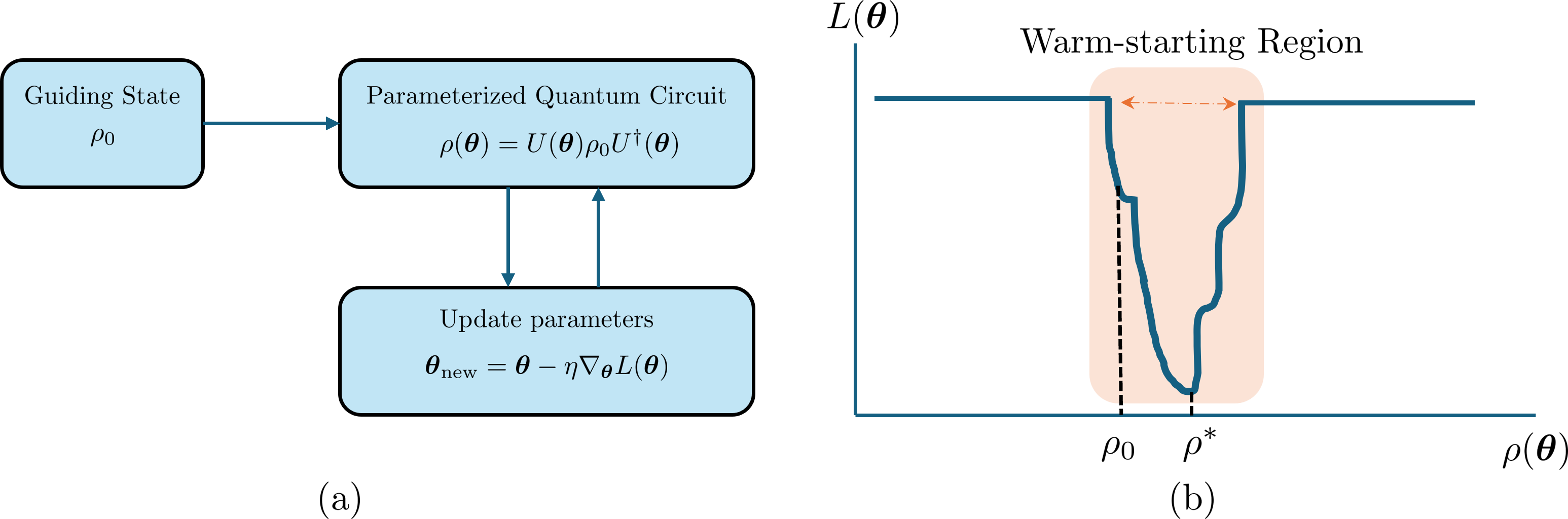
Figure 1: Variational quantum algorithm with guiding state: (a) The algorithm starts with a guiding state as a warm start $\rho_{0}$ and goes through a parameterized quantum circuit $U(\boldsymbol{\theta})$ to learn the representation of the ground state that will be used to generate the properties of the system. The new parameters are updated using gradient descent with learning rate $\eta$ with respect to the loss function $L(\boldsymbol{\theta})$. (b) We present our perspective on warm starts, which is similar to the conventional approach [13]. However, our focus shifts from the initialization of parameters to the initialization of the quantum state itself. It is worth noting that these two approaches can be mapped onto one another.

2 Preliminaries

2.1 Notations

We use bold-faced symbols for vectors. For a vector $\boldsymbol{\theta}$, let $\theta_{j}$ be its $j$-th entry. Similarly, let $A_{ij}$ be the $(i,j)$-th entry of a matrix $A$. We use $\|.\|_{2}$ to denote the Euclidean norm of a vector or Hilbert-Schmidt norm for a matrix and $\|.\|_{\text{op}}$ as operator norm. Let $\lambda(A)$ be the eigenvalues of a matrix $A$. Let I be the identity matrix and $\mathcal{N}(\boldsymbol{\mu},\Sigma)$ be the Gaussian distribution with mean $\boldsymbol{\mu}$ and covariance matrix $\Sigma$.

2.2 Variational Quantum Algorithm

Variational Quantum Algorithms (VQAs) [10] are among the most promising strategies for exploring the practical applications of near-term quantum devices. They typically use a hybrid architecture, where quantum computers evaluate the problem’s cost function, and a classical algorithm optimizes the parameters of the model. Generally, these algorithms define a parameterized quantum circuit (or a quantum ansatz) $U(\boldsymbol{\theta})$ to generate the output state $\rho(\boldsymbol{\theta})$ from an initialized state $\rho_{0}$. The core idea is to minimize a loss function $L(\boldsymbol{\theta})$, which encodes the problem we want to solve. Then classical optimization techniques are employed to iteratively adjust the parameters $\boldsymbol{\theta}$ aiming to find the optimal parameters $\boldsymbol{\theta}^{*}$ that gives the lowest loss value.

One common instance of the optimization algorithm is the gradient descent method, which is intensively used to train classical neural networks [14]. Here, the parameters are updated toward the direction of the steepest descent of the loss function:

$$\boldsymbol{\theta}(t+1)=\boldsymbol{\theta}(t)-\eta\nabla_{\boldsymbol{\theta}}L(\boldsymbol{\theta})$$ (1)

where $\nabla_{\boldsymbol{\theta}}L(\boldsymbol{\theta})$ is the partial gradient vector, $\eta$ is the learning rate parameter controlling the magnitude of the update, and $t$ index the iteration step. The process continues iteratively until the convergence criteria are met. To calculate the partial derivatives $\nabla_{\boldsymbol{\theta}}L(\boldsymbol{\theta})$, one widely used technique in VQAs is the parameter shift rule [41]. This approach evaluates the loss function twice for each parameter:

$$\frac{\partial L(\boldsymbol{\theta})}{\partial\theta_{j}}=\frac{L(\boldsymbol{\theta}+\frac{\pi}{2}\boldsymbol{e}_{j})-L(\boldsymbol{\theta}-\frac{\pi}{2}\boldsymbol{e}_{j})}{2}$$

where $\boldsymbol{e}_{j}$ is the unit vector in the direction of the parameter $\theta_{j}$, meaning it has a $1$ in the $j$-th position and $0$ elsewhere.

The expressive power of VQAs lies in the choice of the quantum ansatz $U(\boldsymbol{\theta})$. Among many candidates, the hardware-efficient ansatz (HEA) [28] appears to be a good solution due to its implementability and expressibility. However, it suffers from a vital problem of barren plateaus [37] where the gradient of the loss function vanishes, making the parameter landscape nearly flat everywhere. This raises the problem of the trainability of VQAs. Another promising choice is alternating layered ansats (ALA) – a specific structure of HEA – which has been proven not to suffer from the vanishing gradient problem in the setting of $\mathcal{O}(\log(n))$ depth [9]. Although the class of ALA is indeed included in that of HEA, the recent result interestingly showed that the shallow ALA has almost the same level of expressibility as that of HEA [43]. Thus, the structure of ALA has both important properties of trainability and expressibility, making it so appealing in the near-term application of quantum computers.

One notable limitation of general VQAs is the difficulty in providing a rigorous performance analysis. Although various studies have been conducted to understand the learning behaviors in training VQAs [57, 20, 3, 31], there are only a few results providing a theoretical performance analysis [17, 49, 34, 8]. Thus, there remains a substantial gap in theoretical analysis in the studies of VQAs.

To address this challenge, it can be helpful to shift focus from parameter spaces to function spaces when understanding learning algorithms. Here, the learning algorithms aim to approximate the target function from a pre-determined hypothesis space. The goal of the learning process is thus to find the best approximation within this space. The critical point is defining a suitable hypothesis space for the problem. In classical approaches, the hypothesis space is built up from typical polynomials (polynomial regression) or composition of linear and non-linear functions (neural network), which are supported by rigorous results that these hypothesis spaces are dense in function space [24, 39]. Meanwhile, the quantum hypothesis space is determined by the various choices of ansatzes. Several studies endeavor to manipulate different quantum ansatzes on function space; for example, quantum signal processing (QSP) [42] provides an ansatz construction to represent any polynomial approximation of the desired function of a unitary. Interestingly, Maria Schuld [50] pointed out that many quantum-supervised learning algorithms are fundamentally kernel methods corresponding to reproducing kernel Hilbert spaces (RKHS). Thus, learning quantum ansatzes is equivalent to learning the ‘quantum kernel’, which generates an RKHS in the target function lies. Inspired by this result, we utilize some tools in kernel theory to provide a rigorous performance analysis of our proposed variational quantum algorithm.

2.3 Neural Tangent Kernel

One particular framework we employ in this work is the neural tangent kernel (NTK) [27, 54]. Let $f_{\boldsymbol{\theta}}$ be the model function defined by the learning algorithm. This function is in a function space $\mathcal{F}$ with respect to a loss function $L:\mathcal{F}\mapsto\mathbb{R}$. Without loss of generality, we assume the learning algorithm is defined on mean square error with respect to a training dataset of $\mathcal{S}=\{(x_{i},y_{i})\}_{i=1}^{M}$:

$$L(\boldsymbol{\theta})=\frac{1}{2M}\sum_{i=1}^{M}(f_{\boldsymbol{\theta}}(x_{i})-y_{i})^{2}.$$

Via gradient descent, the parameters $\boldsymbol{\theta}$ are updated toward the direction of the steepest descent of the loss function:

$$\boldsymbol{\theta}(t+1)=\boldsymbol{\theta}(t)-\eta\nabla_{\boldsymbol{\theta}}L(\boldsymbol{\theta})$$ (2)

If $\eta$ is sufficiently small, we can derive the dynamics of model parameters according to the gradient flow:

$$\frac{d}{dt}\boldsymbol{\theta}(t) =-\eta\nabla_{\boldsymbol{\theta}}L(\boldsymbol{\theta})|_{\boldsymbol{\theta}(t)}$$ (3)

$$=-\frac{\eta}{M}\sum_{i=1}^{M}(f_{\boldsymbol{\theta}(t)}(x_{i})-y_{i})\cdot\nabla_{\boldsymbol{\theta}}f_{\boldsymbol{\theta}}(x_{i})|_{\boldsymbol{\theta}(t)}$$ (4)

As a result, the model function evolves according to:

$$\frac{d}{dt}f_{\boldsymbol{\theta}(t)}(x) =\frac{d}{dt}\boldsymbol{\theta}(t).\nabla_{\boldsymbol{\theta}}f_{\boldsymbol{\theta}}(x)|_{\boldsymbol{\theta}(t)}$$ (5)

$$=-\frac{\eta}{M}\sum_{i=1}^{M}(f_{\boldsymbol{\theta}(t)}(x_{i})-y_{i})\cdot{\nabla_{\boldsymbol{\theta}}f_{\boldsymbol{\theta}}(x_{i})|_{\boldsymbol{\theta}(t)}}^{T}\cdot\nabla_{\boldsymbol{\theta}}f_{\boldsymbol{\theta}}(x)|_{\boldsymbol{\theta}(t)}.$$ (6)

Thus, we can see that the evolution of the model function is indeed governed by a kernel:

$$K_{\boldsymbol{\theta}}(x,x^{\prime}):=\frac{1}{M}{\nabla_{\boldsymbol{\theta}}f(\boldsymbol{\theta},x)|_{\boldsymbol{\theta}}}^{T}\cdot\nabla_{\boldsymbol{\theta}}f(\boldsymbol{\theta},x^{\prime})|_{\boldsymbol{\theta}}$$ (7)

as such:

$$\frac{d}{dt}f_{\boldsymbol{\theta}(t)}(x) =-\eta\sum_{i=1}^{M}(f_{\boldsymbol{\theta}(t)}(x_{i})-y_{i})\cdot K_{\boldsymbol{\theta}(t)}(x_{i},x)$$ (8)

This framework enables us to analyze the algorithm’s behavior through the kernel method. In the context of classical neural networks, Jacot et al. [27] showed that, in the over-parameterized regime, $K_{\boldsymbol{\theta}}$ concentrates around its expectation over random initializations of $\boldsymbol{\theta}$. Moreover, during gradient descent, $K_{\boldsymbol{\theta}}$ remains nearly invariant, a phenomenon known as the lazy training regime. Thus, the optimal values of parameters can be calculated using simple linear estimation. However, due to unitary restriction, this nice property does not hold in the quantum settings [33]. Generally, the quantum neural tangent kernel $K_{\boldsymbol{\theta}}$ still depends on the parameter $\boldsymbol{\theta}$ even in the regime of over-parameterization, making it not applicable with the neural tangent kernel framework. Fortunately, this limitation can be addressed by leveraging the results of [2], which identify the conditions, such as a restricted ansatz class and initial loss conditions, under which the model enters the lazy training regime. Building on this foundation, we develop a unified performance analysis framework for quantum learning models with guiding states, grounded in kernel theory [52] and statistical learning theory [51].

3 Variational Quantum Algorithm with Guiding States

Problem Setup.

We consider the problem of predicting ground state properties of a family of Hamiltonians $H(x)\in\mathbb{C}^{2^{n}\times 2^{n}}$ that is configured by $m$ real parameters $x\in\mathcal{X}$. It can be the coupling constant vectors of Ising models on a fixed lattice or classical nuclear coordinates in electronic molecular Hamiltonians. The goal is to learn a model to predict the properties of ground state $\rho(x)$ from a known observable $O$. In analogy with the QPE setting, we assume access to an oracle that, given an input parameter $x$, outputs a guiding state $\rho_{0}(x)$. This guiding state serves as an approximation to the true ground state and satisfies

$$d_{\Tr}(\rho_{0}(x),\rho(x)):=\frac{1}{2}\|\rho_{0}(x)-\rho(x)\|_{1}\leq\delta\qquad\forall x,$$ (9)

where $\delta$ quantifies the gap in trace distance. In the context of guided local Hamiltonians, it is common to assume $\delta\in\mathcal{O}(1/\text{poly}(n))$ [23, 22]. This assumption is especially relevant to quantum chemistry problems whereby the observation that, in practice, computationally efficient classical techniques often give a fairly good initial approximation of the ground state. In this work, we will keep this term general. It could be either a constant or decay with system size $n$. In addition, although they commonly use fidelity as the measure of closeness between $\rho_{0}(x)$ and $\rho(x)$, this could be easily bounded by the trace distance, ensuring that the established results for guided local Hamiltonian remain valid in our setting.

In particular, we assume the algorithm has access to a training dataset consisting of parameter values $x$ sampled from a distribution $\mathcal{D}$ over $\mathcal{X}$, together with the corresponding ground-state property of $\rho(x)$ with respect to a known observable $O$. Formally, we denote the dataset as

$$\mathcal{S}=\{(x_{i},y_{i})\}_{i=1}^{M},$$ (10)

where $y_{i}=\Tr[O\rho(x_{i})]$. Such data may be generated either from classical simulations or from quantum experiments. Once trained, the quantum algorithm takes as input a new vector $x^{\prime}$ and predicts the observable property $\Tr[O\rho(x^{\prime})]$ of the true ground state $\rho(x^{\prime})$.

Without loss of generality, we equip the learning algorithm with a parameterized quantum circuit $U(\boldsymbol{\theta})$, which is optimized according to the loss function defined for the training dataset $\mathcal{S}$ (10). The loss function is given by:

$$L_{\mathcal{S}}(\boldsymbol{\theta})=\frac{1}{2M}\sum_{i=1}^{M}(f_{\boldsymbol{\theta}}(x_{i})-y_{i})^{2}$$ (11)

where $f_{\boldsymbol{\theta}}(x_{i})=\Tr[O(U(\boldsymbol{\theta})\rho_{0}(x_{i})U^{\dagger}(\boldsymbol{\theta}))]$. Our objective is to optimize $\boldsymbol{\theta}$ to minimize this loss. We focus on the case where $O$ is the sum of few-body operators due to their practical significance in quantum systems where interactions are often confined to a small number of particles. For simplicity, in our analysis, we assume that the observable $O$ is a sum of $k$-local operators $O_{\ell}$, each satisfying $\|O_{\ell}\|_{\text{op}}\leq 1$:

$$O=\frac{1}{{K}}\sum_{\ell=1}^{K}O_{\ell},$$ (12)

where $K$ denotes the number of local terms, typically scaling as $\mathrm{poly}(n)$. The factor $1/{K}$ normalizes $O$ such that $\|O\|_{\text{op}}\leq 1$.

For stability of the model, we also need to assume that the parameterized gates do not vary significantly with small changes in the parameters $\boldsymbol{\theta}$. To ensure this, we assume that:

$$\left\|\frac{\partial}{\partial\theta_{j}}U(\boldsymbol{\theta})\rho_{0}(x)U^{\dagger}(\boldsymbol{\theta})\right\|_{2},\left\|\frac{\partial^{2}}{\partial\theta_{i}\theta_{j}}U(\boldsymbol{\theta})\rho_{0}(x)U^{\dagger}(\boldsymbol{\theta})\right\|_{2}\leq c\ \ \ \forall i,j$$ (13)

for some constant $c>0$.

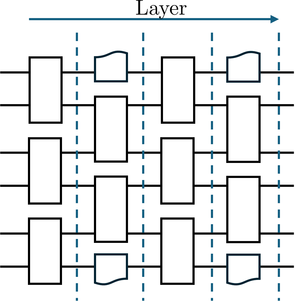
(a)

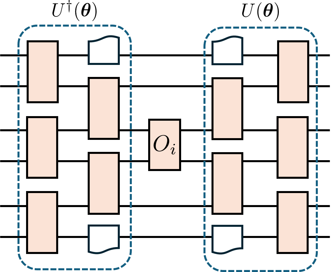
(b)

Figure 2: Alternating Layer Ansatz. (a) An illustration of the alternating layered ansatz. Here, each layer is separated by a vertical dashed line. (b) We illustrate the locality property of ALA. The shaded boxes are in the light cone of $O_{i}$. This means that the actions of $U^{\dagger}(\boldsymbol{\theta})O_{i}U(\boldsymbol{\theta})$ only depend on the parameters in the shaded boxes and the other will be canceled out.

Choice of Quantum Ansatz.

The guarantee of a variational quantum algorithm depends on a variety of factors, including the choice of ansatz $U(\boldsymbol{\theta})$. In this work, we particularly employ alternating layered ansatz (ALA), which has both important properties of trainability and expressibility [43]. The ALA introduced in [9] consists of multiple layers, each of them having some separated blocks that have parameterized single-qubit rotations and a fixed entanglement layer connecting all qubits inside the block. An illustration of the ALA is shown in Figure 2(a). For simplicity, we further assume that each block contains an even number, $m$, qubits ($m$ is independent of $n$), and $n/m$ is an integer. That means in the odd-numbered layer, there are $n/m$ blocks which non-trivially act on $\{1,...,m\},\{m+1,...,2m\},...,\{n-m+1,...,n\}$ qubits, while the even-numbered layer contains $n/m+1$ blocks which acts on $\{1,...,m/2\},\{m/2+1,...,3m/2\},...,\{n-m/2+1,...,n\}$ (the first and the last blocks operate on $m/2$ qubits). In detail, we define the ALA used in our result in Definition 3.

An $n$-qubit unitary $U(\boldsymbol{\theta})$ is ALA($n,m,p,L$) if it consists of $L$ layer where the odd-numbered layer is expressed as:

$$U_{\text{odd}}(\boldsymbol{\theta})=\prod_{i=0}^{n/m-1}W_{[mi+1,m(i+1)]}(\boldsymbol{\theta})_{i}$$

and the even-numbered layer is defined as:

$$U_{\text{even}}(\boldsymbol{\theta})=W_{[n-m/2+1,n]}(\boldsymbol{\theta})_{n/m+1}\prod_{i=0}^{n/m-2}W_{[m(i+1/2)+1,m(i+3/2)]}(\boldsymbol{\theta})_{i}.W_{[1,m/2]}(\boldsymbol{\theta})_{1}$$

where $W_{[a,b]}(\boldsymbol{\theta})$ contains single-qubit rotations and entangler acting on from $a^{th}$ to $b^{th}$ qubits parameterized by $p$ parameters. The advantage of the ALA lies in its co-existence of trainability and expressibility. According to Cerezo et al. [9], an instance of ALA($n,m,p,L$) avoids the issue of barren plateaus if it meets the following criteria: (i) the cost function is defined as a sum of few-body operators, and (ii) the number of layers $L$ scales logarithmically with the system size, specifically $L\in\mathcal{O}(\log(n))$. Remarkably, recent findings indicate that shallow ALA can achieve high expressibility when the ensemble of unitary matrices in each block forms a 2-design [43]. To fulfill this requirement, it is necessary for each block to contain $p\in\mathcal{O}(m)$ parameters to approximate a one-dimensional 2-design [5, 25], while only $\mathcal{O}(\sqrt{m})$ parameters are needed for two-dimensional connectivity [25]. Notably, these parameter requirements do not depend on the total number of qubits $n$. Therefore, the ALA enables us to leverage both trainability and expressibility effectively, even when employing a shallow depth circuit.

Therefore, it is natural to consider $U(\boldsymbol{\theta})\in\text{ALA}(n,m,p,L)$ with $m,L,p=\mathcal{O}(\log(n))$. Under this setting, the model functions generated by ALA exhibit a crucial locality property: the measurement of an observable $O_{i}$ depends only on the light cone of the qubits on which $O_{i}$ acts, as illustrated in Figure 2(b). A formal proof of this statement will be given later (Lemma 5.1). This locality property plays a central role in our main result, which will be established in a subsequent section.

Parameter Initialization.

For parameter initialization, we leverage the guiding states, which give us access to a ‘good’ approximation of the ground state. Instead of randomly initializing the parameters, which could cause the output state to move arbitrarily across the Hilbert space, we initialize the parameters near the vector $\boldsymbol{0}$. Specifically, we model the initialized parameters as drawn from a Gaussian distribution:

$$\boldsymbol{\theta}(0)\sim\mathcal{N}(\boldsymbol{0},\kappa^{2}\mathbf{I})$$ (14)

where $0<\kappa\leq 1$ controls the magnitude of initialization, and all randomnesses are independent. This initialization strategy serves two key purposes. First, this avoids the output state being distributed randomly due to the high expressibility of ALA. Second, it allows us to take advantage of the guide state that is already close to the ground state, so this initialized scheme will put the output state into a more favorable region near the optimal value.

Putting it all together.

Our algorithm is then described as follows:

Algorithm 1 Variational Quantum Algorithm with guiding states

1:Input:

• Training data $\mathcal{S}$ (10) defined on a system size $n$

• Observable $O$ (12)

• Circuit configurations $m,p,L$, which are $\mathcal{O}(\log(n))$

• Learning rate $\eta$

• Number of iterations $T$

2:Output: Trained model $\boldsymbol{\theta}$

3:Initialize the ALA($n,m,p,L$) circuit with parameters $\boldsymbol{\theta}\sim\mathcal{N}(\boldsymbol{0},\kappa^{2}\mathbf{I})$

4:for t = 1 to $T$ do

5:  for i = 1 to $M$ do $\triangleright$ M is the number of training samples in $\mathcal{S}$

6:   $\hat{y}_{i}\leftarrow\text{Forward the circuit with }\rho_{0}(x_{i})$

7:  end for

8:  $L_{\mathcal{S}}(\boldsymbol{\theta})\leftarrow\text{Compute loss function as~\eqref{eqn: loss_function}}$

9:  $\nabla_{\boldsymbol{\theta}}L_{\mathcal{S}}(\boldsymbol{\theta})\leftarrow\text{Compute gradients of }\boldsymbol{\theta}\text{ w.r.t $L_{\mathcal{S}}(\boldsymbol{\theta})$}$

10:  $\boldsymbol{\theta}(t+1)\leftarrow\boldsymbol{\theta}(t)-\eta\nabla_{\boldsymbol{\theta}}L_{\mathcal{S}}(\boldsymbol{\theta})$ $\triangleright$ Update parameters

11:end for

12:return $\boldsymbol{\theta}$

4 Theoretical Guarantees

In this section, we present the main results of our study, focusing on both the convergence properties and generalization performance of Algorithm 1. We begin by analyzing the convergence behavior, which is followed by a detailed examination of its generalization capabilities. Our results on convergence and generalization will crucially depend on the spectrum of the neural tangent kernel at initialization $K_{\boldsymbol{\theta}(0)}$.

4.1 Convergence

The key to our convergence analysis is the observation that, given the guiding states, it only requires a small initialization magnitude of $\kappa$ to establish the neural tangent kernel theory for Algorithm 1. Its convergence analysis is the following: [Convergence] Under the training as Algorithm 1, suppose $0\leq\lambda_{\text{min}}:\lambda_{\text{min}}(K_{\boldsymbol{\theta}(0)})\leq\lambda_{j}\leq\lambda_{\text{max}}:=\lambda_{\text{max}}(K_{\boldsymbol{\theta}(0)})\leq\infty$ and for $\eta=\mathcal{O}(\frac{\lambda_{\text{min}}}{M^{2}})$, $\kappa=\tilde{\mathcal{O}}(\frac{\delta\sqrt{\gamma}}{n})$. Then, with probability at least $1-\gamma$ over the random initialization, we have for all $t>0$:

$$L_{\mathcal{S}}(\boldsymbol{\theta}(t))=\tilde{\mathcal{O}}\left(\sum_{j}(1-\eta\lambda_{j})^{2t}\delta^{2}+\frac{n}{K^{3}}\eta^{2}t^{2}\delta^{3}\right)$$

In light of this result, the dominant term $\sum_{j}(1-\eta\lambda_{j})^{2t}\delta^{2}$ vanishes as $t$ increases. Convergence is faster along directions associated with larger eigenvalues $\lambda_{j}$, consistent with findings in the classical neural tangent kernel (NTK) setting [27]. Intuitively, larger eigenvalues correspond to directions in parameter space where the loss surface has steeper curvature, leading to more rapid error reduction. This behavior mirrors the dynamics of linear models and the NTK approximation, where convergence is primarily governed by the learning rate $\eta$ and the spectrum of the tangent kernel. In contrast, directions associated with smaller eigenvalues converge more slowly, producing a staggered convergence pattern across different parameter dimensions.

The correction term $\tfrac{n}{K^{3}}\eta^{2}t^{2}\delta^{3}$, by comparison, grows quadratically in $t$. This growth is mitigated by the denominator $K^{3}$, which scales polynomially in $n$, ensuring that its contribution is suppressed as system size increases. Moreover, the use of guiding states also reduces the number of update steps $t$ needed, further controlling this term. Taken together, these effects guarantee that the correction term remains secondary, so that convergence is ultimately driven by the spectral dynamics, providing both stability and scalability in our variational quantum algorithm.

4.2 Generalization Error

We next provide the generalizability of the learning model in Algorithm 1. In particular, we study the theoretical bound for the generalization error, which is defined as:

$$\text{gen}(\boldsymbol{\theta}):=\left|\mathbb{E}_{x\sim\mathcal{D}}[\left|f_{\boldsymbol{\theta}}(x)-\Tr[O\rho(x)]\right|]-\mathbb{E}_{x\sim\mathcal{S}}[\left|f_{\boldsymbol{\theta}}(x)-\Tr[O\rho(x)]\right|]\right|.$$ (15)

The following theorem establishes the theoretical bound of the generalization error of the Algorithm 1: [Generalization] Consider a training dataset $\mathcal{S}$ (10) defined on a system size $n$ with the observable $O$ is represented as (12). If the Algorithm 1 is trained on $\mathcal{S}$ with $\eta=\mathcal{O}(\frac{\lambda_{\text{min}}}{M^{2}})$ and $\kappa=\tilde{\mathcal{O}}(\frac{\delta\sqrt{\gamma}}{n})$, there exists $B_{1},B_{2}$ such that with $T=\Theta\left(\log_{(1-\eta\lambda_{\text{min}})}{\frac{1}{M}}\right)$ iterations, then $B_{1}\leq\Tr[e^{-\eta TK_{\boldsymbol{\theta}(0)}}]\leq B_{2}$. And for a confidence parameter $\gamma\in(0,1)$,

$$\text{gen}(\boldsymbol{\theta})\leq\tilde{\mathcal{O}}\left(B_{2}\delta\sqrt{\frac{1}{M}}+\sqrt{\frac{\ln(1/\gamma)}{M}}+\frac{n}{K^{3}}\eta^{2}\left(\log_{(1-\eta\lambda_{\text{min}})}{\frac{B_{1}}{M}}\right)^{2}\delta^{3}\right)$$

with a probability at least $1-\gamma$ over the random initialization, where $\lambda_{\text{min}}$ is the smallest eigenvalues of the initialized tangent kernel $K_{\boldsymbol{\theta}(0)}$ defined in (7). Now, we discuss our generalization bound. The dominating term is:

$$B_{2}\delta\sqrt{\frac{1}{M}}.$$

The value of $B_{2}$ plays a crucial role in controlling the generalization error and indicates the behavior of the trace of the matrix exponential, $e^{-\eta TK_{\boldsymbol{\theta}(0)}}$. $B_{2}$ indeed provides an upper bound on the trace of the matrix that governs the convergence behavior of the algorithm, which highly depends on the spectrum of $K_{\boldsymbol{\theta}(0)}$. If $B_{2}$ is independent of the number of samples $M$, then when the system size is large enough, we can obtain the generalization error, $\text{gen}(\boldsymbol{\theta})\leq\epsilon$ with $\mathcal{O}(\frac{B^{2}_{2}\delta^{2}+\log(1/\gamma)}{\epsilon^{2}})$ training data.

On the other hand, the model’s efficiency in general settings is strongly influenced by the eigensystem of the kernel $K_{\boldsymbol{\theta}(0)}$. In the worst case, this may require an impractically large amount of training data for good performance. However, this requirement can be substantially reduced by selecting an appropriate kernel. The central challenge lies in identifying a kernel that effectively encodes the relevant structure of the problem. Kernel design reflects how prior knowledge is embedded and exploited, yet determining the right inductive bias is often nontrivial [51]. The difficulty stems from the need to express the inductive bias that best aligns with the data’s underlying structure. Several works have investigated ways to incorporate such inductive bias into quantum kernels [49, 30, 34]. We further remark that Theorem 4.2 suggests an alternative route to inducing inductive bias—through the spectrum of the tangent kernel. If this spectral bias can be properly controlled, it has the potential to accelerate both training and generalization.

We again emphasize the role of guiding states in our algorithm. The quality of the guiding state, captured by the parameter $\delta$, directly influences the generalization bound through the additional term

$$\frac{n}{K^{3}}\eta^{2}\left(\log_{(1-\eta\lambda_{\text{min}})}{\frac{B_{1}}{M}}\right)^{2}\delta^{3}.$$

This contribution is most relevant in regimes where the system size $n$ is finite but large. While the factor $\frac{n}{K^{3}}$ ensures that its impact diminishes as the system grows, for smaller $n$ the term can dominate if the guiding state is of poor quality (i.e., $\delta$ is large). The cubic dependence on $\delta$ underscores how strongly the accuracy of the guiding state affects the generalization behavior. In the context of guided local Hamiltonian problems, where $\delta=\mathcal{O}(1/\mathrm{poly}(n))$, this effect becomes particularly favorable. High-quality guiding states suppress the additional term, making the bound more favorable even at modest system sizes.

Finally, our result also informs the relationship between the number of training data and the number of gradient descent iterations in Algorithm 1. As our choice of $\eta=\mathcal{O}(\lambda_{\text{min}}/M^{2})$, this implies $\mathbf{I}-\eta K_{\boldsymbol{\theta}(0)}$ is positive semidefinite. Then, $0\leq 1-\eta\lambda_{\text{min}}\leq 1$ must hold. Therefore, if the number of training data $M$ increases, the value of $T$ tends to decrease as

$$T=\Theta\left(\log_{(1-\eta\lambda_{\text{min}})}{\frac{1}{M}}\right).$$

In other words, with more training data, the algorithm requires fewer iterations to achieve convergence.

5 Proof Ideas

In this section, we outline the key ideas behind the proofs of Theorem 4.1 and Theorem 4.2. The central component of the proof is the concentration property of the quantum neural tangent kernel with ALA, which will be fully described in Appendix A. This result enables us to approximate the model dynamics by their linear approximation, obtained via a first-order Taylor expansion around the initialization, which is a step we refer to as the linearization trick. Building on this approximation, we then apply standard tools from learning theory to derive guarantees on both convergence and generalization. The complete technical arguments are provided in Appendix B.

5.1 Concentration of Quantum Neural Tangent Kernel

We show that if $U(\boldsymbol{\theta})$ is alternating layered ansatz (Definition 3) with initialization scheme as (14), $K_{\boldsymbol{\theta}}$ is concentrated into a limiting kernel and stays constant via gradient descent algorithms as the system size $n$ goes to infinity. Shown in Algorithm 1, we consider the setting of ALA($n,m,p,L$) with $m,p,L\in\mathcal{O}(\log(n))$. Then, let us first discuss the locality lemma regarding our ALA design. Let a parameterized quantum circuit $U(\boldsymbol{\theta})\in\text{ALA}(n,m,p,L)$. For any $k$-local observable $O$ such that $m\geq k$, $U^{\dagger}(\boldsymbol{\theta})OU(\boldsymbol{\theta})$ acts non-trivially on $\mathcal{O}(Lm)$ qubits.

Proof.

Let $S_{V}$ as the support of operator $V$. Denote $W_{L}$ is the block at the last layer such that $S_{O}\subseteq S_{W_{L}}$. We are interested in finding the locality of $O(\boldsymbol{\theta})=U^{\dagger}(\boldsymbol{\theta})OU(\boldsymbol{\theta})$. Noting that, for each layer $S_{O(\boldsymbol{\theta})}$ is extended by $2m$ qubits. So the locality of $O(\boldsymbol{\theta})$ is $\mathcal{O}(Lm)$. ∎

Since $L$ and $m$ are in $\mathcal{O}(\log(n))$, the model function of a $k$-local observable will act non-trivially on qubits in $\mathcal{O}(\log(n)^{2})$-size light cones. This locality property of the model function $f_{\boldsymbol{\theta}}$ will aid in proving the convergence of $K_{\boldsymbol{\theta}}$. Specifically, we can show that for any initialization of $\boldsymbol{\theta}$, the tangent kernel entry $K_{\boldsymbol{\theta}}$ defined by ALA will concentrate around its mean.

[Concentration of initialization] Consider Algorithm 1, for any initialization distribution of $\boldsymbol{\theta}\in\mathbb{R}^{L\times p\times n/m}$, the tangent kernel (7) satisfies:

$$\mathbb{P}_{\boldsymbol{\theta}}[\left|K_{\boldsymbol{\theta}}(x,x^{\prime})-\mathbb{E}_{\boldsymbol{\theta}}[K_{\boldsymbol{\theta}}(x,x^{\prime})]\right|\geq\epsilon] \leq\exp{-\Omega\left(\frac{M^{2}\epsilon^{2}}{c^{4}}\cdot\frac{K^{4}}{n\cdot\text{poly}(\log(n))}\right)}$$ (16)

The theorem shows that the quantum neural tangent kernel is concentrated when the system size $n$ is large, since $K=\mathrm{poly}(n)$. This immediately implies that at the limit of infinite width $n$, the tangent kernel converges to a limit kernel.

Next, we need to prove that $K_{\boldsymbol{\theta}}$ stays constant during the gradient descent iterations. Leveraging the fact that Theorem 5.1 is true for any initialization scheme $\boldsymbol{\theta}$. Our initialization scheme in Algorithm 1 results the following theorem: [Lazy Training] Suppose $\boldsymbol{\theta}(0)\sim\mathcal{N}(\boldsymbol{0},\kappa^{2}\mathbf{I})$ with $\kappa\in\tilde{\mathcal{O}}(\frac{\sqrt{\gamma}\delta}{n})$, then during gradient descent algorithm via loss function (11), any single entry $K_{ij}(\boldsymbol{\theta})$ of the tangent kernel $K_{\boldsymbol{\theta}}$ (7) is updated in time by:

$$\left|\frac{d}{dt}K_{ij}(\boldsymbol{\theta}(t))\right|\leq\tilde{\mathcal{O}}\left(\frac{\eta^{2}\delta n}{M\cdot K^{3}}\right)\ \ \ \forall i,j$$

with probability at least $1-\gamma$ over the random initialization. Note that we keep $\delta$ in a general form. It could be either a constant or decay with the system size $n$ as in guided local Hamiltonian literature, e.g., $\delta\in\mathcal{O}(1/\text{poly}(n))$. In both cases, Theorem 5.1 shows that the change of quantum neural tangent kernel after each iteration of the gradient descent algorithm is inverse polynomial in terms of $n$, as $K$ scales polynomially in $n$. This implies the kernel $K_{\boldsymbol{\theta}}$ asymptotically stays constant during training.

5.2 Convergence and Generalization

From Theorem 5.1 and Theorem 5.1, we could use results from kernel theory [52] to analyze the performance of our model. The key to this part is that we simplify the model to its linear approximation when the system size is large enough. To see this, we define a linear model as the first-order Taylor expansion of the model function with respect to the parameters around its initialization:

$$\hat{f}_{\boldsymbol{\theta}}:=f_{\boldsymbol{\theta}(0)}+\nabla_{\boldsymbol{\theta}}f_{\boldsymbol{\theta}}|_{\boldsymbol{\theta}(0)}.(\boldsymbol{\theta}-\boldsymbol{\theta}(0))$$ (17)

For brevity, we omit the inputs in this analysis. Given $\boldsymbol{\theta}(0)$, $f_{\boldsymbol{\theta}(0)}$ and $\nabla_{\boldsymbol{\theta}}f_{\boldsymbol{\theta}}|_{\boldsymbol{\theta}(0)}$ are all constant, assuming the update step $\eta$ is small enough, the parameters of the linearized model are updated by gradient descent the same loss function (11):

$$\frac{d}{dt}\boldsymbol{\theta}(t) =-\eta\nabla_{\boldsymbol{\theta}}L_{\mathcal{S}}(\boldsymbol{\theta})|_{\boldsymbol{\theta}(t)}$$ (18)

$$\frac{d}{dt}\boldsymbol{\theta}(t) =-\frac{\eta}{M}\sum_{i=1}^{M}(\hat{f}_{\boldsymbol{\theta}(t)}(x_{i})-y_{i})\cdot\nabla_{\boldsymbol{\theta}}\hat{f}_{\boldsymbol{\theta}}|_{\boldsymbol{\theta}(t)}$$ (19)

$$\frac{d}{dt}\boldsymbol{\theta}(t) =-\frac{\eta}{M}\sum_{i=1}^{M}(\hat{f}_{\boldsymbol{\theta}(t)}(x_{i})-y_{i})\cdot\nabla_{\boldsymbol{\theta}}f_{\boldsymbol{\theta}}|_{\boldsymbol{\theta}(0)}$$ (20)

$$\frac{d}{dt}\hat{f}_{\boldsymbol{\theta}(t)} =-\frac{\eta}{M}\sum_{i=1}^{M}(\hat{f}_{\boldsymbol{\theta}(t)}(x_{i})-y_{i})\cdot{\nabla_{\boldsymbol{\theta}}f_{\boldsymbol{\theta}}|_{\boldsymbol{\theta}(0)}}^{T}.\nabla_{\boldsymbol{\theta}}f_{\boldsymbol{\theta}}|_{\boldsymbol{\theta}(0)}$$ (21)

$$\frac{d}{dt}\hat{f}_{\boldsymbol{\theta}(t)} =-\eta\sum_{i=1}^{M}(\hat{f}_{\boldsymbol{\theta}(t)}(x_{i})-y_{i})\cdot K_{\boldsymbol{\theta}(0)}$$ (22)

Eventually, we recover the same learning dynamics as those of the original model (8). According to Theorems 5.1 and 5.1, the kernel $K_{\boldsymbol{\theta}}$ exhibits strong concentration properties and remains effectively constant throughout the gradient descent trajectory. Consequently, in the infinite-width (or large-system) limit, we have $K_{\boldsymbol{\theta}(0)}=K_{\boldsymbol{\theta}(t)}$ for all $t$, indicating that the training dynamics are governed by a fixed kernel. This observation implies that, as the system size approaches infinity, the true nonlinear model converges to its linearized counterpart, validating the linear approximation regime.

We now proceed to analyze the convergence behavior of this linearized model (22), as formalized in the following theorem.

Consider Algorithm 1, and let the eigenvalues of the kernel matrix $K_{\boldsymbol{\theta}(0)}$ satisfy $0\leq\lambda_{\min}:=\lambda_{\min}(K_{\boldsymbol{\theta}(0)})\leq\lambda_{j}\leq\lambda_{\max}:=\lambda_{\max}(K_{\boldsymbol{\theta}(0)})<\infty.$ For a learning rate $\eta\in\mathcal{O}\!\left(\frac{\lambda_{\min}}{M^{2}}\right)$ and parameter $\kappa\in\tilde{\mathcal{O}}\!\left({\sqrt{\gamma}\,\delta/n}\right)$, let $\hat{L}_{\mathcal{S}}(\boldsymbol{\theta}(t))$ denote the empirical loss of the model evolving under the linearized dynamics (22) at time $t$. Then, the loss satisfies

$$|\hat{L}_{\mathcal{S}}(\boldsymbol{\theta}(t))|\leq\tilde{\mathcal{O}}\!\left(\sum_{j}(1-\eta\lambda_{j})^{2t}\,\delta^{2}\right).$$

However, the true model coincides with its linear approximation only in the limit of infinite system size. Our interest lies instead in the practically relevant case of finite $n$. We therefore establish the following training error bound between the true model and its linear approximation: Consider the Algorithm 1 trained on a dataset $\mathcal{S}$ (10) and loss function (11). Suppose $\eta=\mathcal{O}(\frac{\lambda_{\text{min}}}{M^{2}})$, $\kappa\in\tilde{\mathcal{O}}(\frac{\sqrt{\gamma}\delta}{n})$ and let $L_{\mathcal{S}}^{*}(\boldsymbol{\theta}(t))$ be the model loss of the true dynamics governed by the time-variance kernel $K_{\boldsymbol{\theta}(t)}$ (7) and $\hat{L}_{\mathcal{S}}(\boldsymbol{\theta}(t))$ be the model loss of the asymptotic dynamics governed by the initialized kernel $K_{\boldsymbol{\theta}(0)}$ (22), we have:

$$\left|L_{\mathcal{S}}^{*}(\boldsymbol{\theta}(t))-\hat{L}_{\mathcal{S}}(\boldsymbol{\theta}(t))\right|\leq\tilde{\mathcal{O}}\left(\frac{n}{K^{3}}\eta^{2}t^{2}\delta^{3}\right)$$ (23)

Combining Theorem 5.2 and Theorem 23, we derive the convergence result in Theorem 4.1.

The result in Theorem 23 will also help us derive the theoretical bound of the generalization error of the true model. Particularly, we will provide generalization bounds based on the Rademacher complexity [51]. Generally, Rademacher complexity is a measure used in statistical learning theory to quantify the ability of a class of functions to fit random noise. It evaluates the richness of a function class by calculating the average correlation between the functions and random Rademacher variables, which take values of +1 or -1 with equal probability. Lower Rademacher complexity indicates a less flexible model, typically leading to better generalization from training data to unseen data. Due to the concentration of tangent kernel at the infinite-width limit, the class of functions of the model is well-characterized by famous kernel methods [52].

Specifically, we consider a set of independent samples $\mathcal{S}=\{x_{1},...,x_{M}\}$ such that $x_{i}$ is drawn from an unknown distribution $\mathcal{D}$. Let us define $\mathcal{F}$ to be the set of functions that could be learned from a learning model. The Rademacher complexity theory allows us to obtain the bounds of generalization error associated with learning from training data [51]. For convenience, we denote $\ell(f_{\boldsymbol{\theta}}(x))=\left|f_{\boldsymbol{\theta}}(x)-\Tr[O\rho(x)]\right|$, the Rademacher complexity of a function space $\ell\circ\mathcal{F}$ with respect to training data $\mathcal{S}$ is defined as follows:

$$R(\ell\circ\mathcal{F}\circ\mathcal{S}):=\frac{1}{M}\mathbb{E}_{\boldsymbol{\sigma}\in\{-1,1\}^{M}}\left[\sup\sum_{i=1}^{M}\sigma_{i}\ell(f_{\boldsymbol{\theta}(t)}(x_{i}))\right]$$ (24)

This quantity provides a bound on the generalization error by the following lemma [Theorem 26.5 [51]] For a training sample $\mathcal{S}=\{x_{1},\dots,x_{M}\}$ generated by an unknown distribution $\mathcal{D}$ and real-value function class $\mathcal{F}$, such that for all $x$ and $f\in\mathcal{F}$ we have $|\ell(f(x))|\leq c$. Then, for a confidence parameter $\gamma\in(0,1)$, with probability at least $1-\gamma$ over the random initialization, every $f\in\mathcal{F}$ satisfies:

$$\mathbb{E}_{x\sim\mathcal{D}}[\ell(f(x))]-\mathbb{E}_{x\sim\mathcal{S}}[\ell(f(x))]\leq 2R(\ell\circ\mathcal{F}\circ\mathcal{S})+4c\sqrt{\frac{2\ln(4/\gamma)}{M}}$$

The lemma shows that the generalization error is upper-bounded by the Rademacher complexity. If the quantity $R(\ell\circ\mathcal{F}\circ\mathcal{S})$ is small, then we could reliably learn the target function. Thus, we next aim to bound this quantity. First, we consider the Rademacher complexity of the function class, $\hat{\mathcal{F}}$, as the set of functions generated by the initialization kernel $K_{\boldsymbol{\theta}(0)}$ based on the dynamics in (22). Then, we analyze the asymptotic result of the true function class, $\mathcal{F}^{*}$, generated by time-dependent kernel $K_{\boldsymbol{\theta}(t)}$ (8).

As pointed out in [27] and our result in Theorem 4.1, we see that the convergence of the tangent kernel model is faster along the eigenspaces with larger eigenvalues $\lambda_{i}$ of $K_{\boldsymbol{\theta}(0)}$. We are typically interested in the case where the model focuses on fitting the most relevant kernel principal components (larger eigenvalues), which is the motivation for the use of early stopping. Thus, for the analysis of Rademacher complexity, we consider the function class with a bounded sum of eigenvalues:

$$(\ell\circ\mathcal{F})_{B}:=\{\ell_{t}\in\ell\circ{\mathcal{F}}|B_{1}\leq\sum_{i}e^{-t\eta\lambda_{i}}\leq B_{2}\}$$

From that, we can bound the Rademacher complexity to the function class of the linear model in (22) as:

$$R((\ell\circ\hat{\mathcal{F}})_{B}\circ\mathcal{S})\leq B_{2}\sqrt{\frac{2}{M}L_{\mathcal{S}}(\boldsymbol{\theta}(0))}$$

which brings us to its generalization error as:

$$\text{gen}_{\text{linear}}(\boldsymbol{\theta})\leq 2B_{2}\sqrt{\frac{2}{M}L_{\mathcal{S}}(\boldsymbol{\theta}(0))}+4c\sqrt{\frac{2\ln(4/\gamma)}{M}}$$ (25)

with probability at least $1-\gamma$ over the random initialization, where $\text{gen}_{\text{linear}}(\boldsymbol{\theta})$ defines the generalization error of the linear model.

Finally, we compare the Rademacher complexity of the true model with its linear approximation as such:

$$|R((\ell\circ\mathcal{F}^{*})_{B}\circ\mathcal{S})-R((\ell\circ\hat{\mathcal{F}})_{B}\circ\mathcal{S})|\leq\tilde{\mathcal{O}}\left(\frac{n}{K^{3}}\eta^{2}\left(\log_{(1-\eta\lambda_{\text{min}})}{\frac{B_{1}}{M}}\right)^{2}\delta^{3}\right)$$ (26)

Combining the results from (25) and (26), we establish the bound in Theorem 4.2. The detailed proofs for (25) and (26) are presented in Appendix B.

6 Numerical Analysis

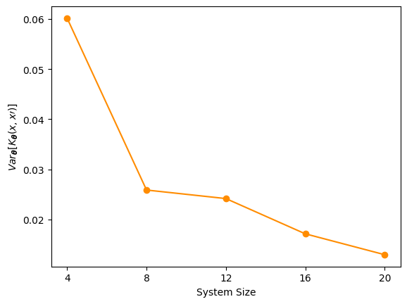
(a) Kernel entry

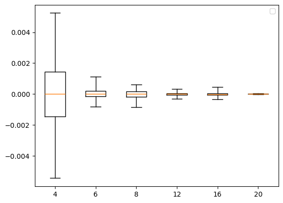
(b) Evolution of kernel entry

(c) Training behavior

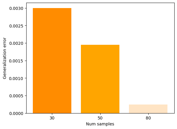
(d) Generalization error

Figure 3: Predicting ground state properties in 2D antiferromagnetic random Heisenberg models. (a) The variance of a single entry $K_{\boldsymbol{\theta}(0)}(x,x\prime)$ over $100$ different initialization in a variety of system sizes $n$. The experiment corresponds to the ALA with $L=1$ and $m=2$. (b) The distribution of $\frac{d}{dt}K_{\boldsymbol{\theta}}(x,x\prime)$ across different system size settings $n$ over a range of $t$ from $1$ to $100$. As the system size goes to $20$, the values $K_{\boldsymbol{\theta}}(x,x\prime)$ asymptotically stays constant. (c) Training behavior of the true model corresponding to linearized model with initialized kernel $K_{\boldsymbol{\theta}(0)}$. The models are performed with ALA$(n=20,m=4,L=2)$. (d) The generalization error with three different training dataset sizes of $30,50,80$.

In this section, we present numerical experiments to assess the performance of our algorithm in practice. Here, we consider the two-dimensional anti-ferromagnetic Heisenberg model with Hamiltonian of:

$$H(x)=\sum_{\langle ij\rangle}x_{ij}(X_{i}X_{j}+Y_{i}Y_{j}+Z_{i}Z_{j})$$

where the sum is over the nearest neighbors in a 2D lattice, which accounts for the interaction between each pair of adjacent spins. The values of $x=(x_{ij})_{i,j}^{n}$ represent the coupling matrix determining the strength of the interactions. For any observable $O$, the goal is using Algorithm 1 to produce a hypothesis $f_{\boldsymbol{\theta}}$ such that:

$$f_{\boldsymbol{\theta}}(x)=\bra{\psi(x)}O\ket{\psi(x)}$$

where $\ket{\psi(x)}$ denotes the ground state of $H(x)$. In these experiments, we focus on the Hamiltonian $H(x)$ on a $2\times 10$ lattices. The dataset is generated by uniformly sampling the coupling constant $\{x_{ij}\}$ at random from the interval $[0,2]$. We train our Algorithm 1 on a training dataset of $80$ randomly chosen values of $x=\{x_{ij}\}$ and validate on a $20$-sample testing dataset. The algorithm will aim to predict the ground state properties of $O=\frac{1}{\sqrt{n}}\sum_{i=1}^{n}Z_{i}$, where $n$ is the number of qubits. In each sample, the guiding state is generated as follows:

$$\ket{\psi_{0}(x)}=(1-\delta)\ket{\psi(x)}+\delta\ket{\psi^{\perp}(x)}$$

where $\ket{\psi^{\perp}(x)}$ is one of the excited states of the Hamiltonian $H(x)$ and $\delta$ defines the closeness between the initial state and the ground state, which is set as $1/n^{2}$. The implementation is available in [1].

In the following, we characterize our theoretical claims. These first include analyzing the convergence of the quantum neural tangent kernel in our construction and learning behaviors of the true model with respect to the linearized model governed by the initialized tangent kernel. Then, we validate the generalization error of our algorithm.

In Figure 3(a), we show the variance of a single kernel entry at over $100$ random initialization of $\boldsymbol{\theta}$. Note that Theorem 5.1 holds for any initialization scheme, so it will not affect our parameter initialization strategy in Algorithm 1. We can see that as the system size increases, the deviation of the tangent kernel entry decreases, indicating that the kernel entries become more concentrated around their mean. To demonstrate the convergence of the quantum neural tangent kernel, we further illustrate the amount of $\frac{d}{dt}K_{\boldsymbol{\theta}}(x,x^{\prime})$ over the range of $t$ from 1 to 100 when training with the Algorithm 1 in Figure 3(b). The figure shows the distribution of the updates of elements in the tangent kernel at different system sizes. We can see that the median (orange line) is close to zero for all system sizes, indicating that the central tendency of the data is near zero, regardless of the system size. As the system size increases, the width of the boxes tends to decrease, meaning the values become more concentrated around the mean, which is close to zero. This suggests that the values of $\frac{d}{dt}K_{\boldsymbol{\theta}}(x,x^{\prime})$ tend to approach zero as the system size approaches infinity.

The two first experiments help us to see clearly the convergence of the quantum neural tangent kernel that will support us in analyzing the performance of our true model through the linearized model described in (22). In particular, we are interested in the training and generalization error of our algorithm in Figures 3(c) and 3(d). For these experiments, we work with the system size of $20$ and train the algorithm with the alternating layered ansatz of $m=4$ and $L=2$ and run with 100 training iterations. First, we analyze the asymptotical training behavior of the model compared to the linearized model governed by the initialized kernel $K_{\boldsymbol{\theta}(0)}$ (22). In Figure 3(c), we can see that the training error of the model asymptotically behaves similarly to its linearized version, demonstrating our Theorem 23. That means when the system size is large enough, the performance of the linearized model could well-characterize the true model. Next, we study the generalization error of the model training with our Algorithm 1 for different training dataset sizes $M$. As seen in Figure 3(d), the generalization error drops significantly with the number of training samples $M$.

7 Conclusion and Open Problems

This paper introduces a guiding state variational quantum algorithm (VQA) for predicting ground-state properties and develops a proof technique based on a linearization trick to analyze its performance. By establishing a concentration property of the training dynamics, we show that the algorithm can be approximated by a kernel model, enabling rigorous guarantees on both convergence and generalization. Our analysis highlights the critical role of guiding states: they accelerate convergence, suppress finite-size error terms, and ensure stability across system dimensions. While their influence vanishes asymptotically as the system size $n$ grows, for practically relevant moderate-scale systems, high-quality guiding states remain essential for efficient learning and reliable generalization.

Our analysis shows that convergence in parameter space is heavily influenced by the spectrum of the model’s tangent kernel. This result also opens up several avenues for further theoretical investigation. Firstly, our findings might suggest a new approach for inducing inductive bias in quantum learning models by controlling the spectrum of the tangent kernel. This concept has been previously explored in classical neural tangent kernels [4, 48, 21]. Secondly, there is potential to leverage the equivalence between quantum learning models and their linear counterparts, particularly for large system sizes. One could develop a hybrid model that utilizes quantum computers to calculate $K_{\boldsymbol{\theta}(0)}$ while employing classical algorithms to learn the linear model. This approach could be compared to classical algorithms [26], which require specific assumptions about the Hamiltonian, such as a constant spectral gap, while our proposed method might not necessitate such constraints.

However, our algorithm relies on the initialization of guiding states and the ALA of $\mathcal{O}(\log(n))$ depth, which generally raises several important challenges. First of all, obtaining the guiding state is not always straightforward. Even though guiding states are known for specific restricted cases [55], the effort required to locate a near-optimal input state in general can be significant—often enough to negate the efficiency gains of our method. This leads to a fundamental question: does the complexity of finding a good initialization merely shift the burden from training a variational quantum algorithm to precomputing an effective starting point? Additionally, there is the question of whether the proposed algorithm contributes to a genuine quantum advantage. If warm-started variational quantum algorithms operate in a parameter regime where classical methods can efficiently approximate their behavior, then their computational benefits may be limited. Recent studies suggest that quantum circuits in well-optimized regions may be classically simulable, raising concerns about whether warm starts truly enable access to classically intractable solutions [13].

While our analysis does not provide a definitive resolution to these questions, it highlights an important perspective: the proposed algorithm can serve as a conceptual bridge, motivating the design of quantum-inspired algorithms that leverage guiding state and linearized dynamics. In this way, even if their direct quantum advantage remains uncertain, our framework helps clarify where quantum resources are truly necessary and where classical analogues may suffice.

Acknowledgments.

We thank Thinh Le, Mingyu Sun, and Gabriel Waite for valuable discussions related to this work. We are also grateful to Marco Cerezo, Amira Abbas, Samuel Elman, and the anonymous reviewers for their constructive feedback. TN is supported by a scholarship from the Sydney Quantum Academy, PHDR06031.

Appendix A Concentration of Quantum Neural Tangent Kernel

A.1 Concentration at initialization

We will start by proving that at the limit of infinite width, the quantum neural tangent kernel (7) defined by the ALA concentrates around its means and stays constant along with gradient descent updates. [Concentration of initialization] Consider the dataset $\mathcal{S}$ (10) and loss function (11) with the model function defined on $U(\boldsymbol{\theta})\in\text{ALA}(n,m,p,L)$, then for any initialization distribution of $\boldsymbol{\theta}\in\mathbb{R}^{L\times p\times n/m}$, the entry in the tangent kernel (7) satisfies:

$$\mathbb{P}_{\boldsymbol{\theta}}[\left|K_{\boldsymbol{\theta}}(x,x^{\prime})-\mathbb{E}_{\boldsymbol{\theta}}[K_{\boldsymbol{\theta}}(x,x^{\prime})]\right|\geq\epsilon] \leq\exp{-\Omega(\frac{M^{2}K^{4}\epsilon^{2}}{L^{3}pnmc^{4}})}$$ (27)

for all $x,x^{\prime}\in\mathcal{S}$.

Proof.

The proof adapts from Theorem 1 [2]. Consider the model function:

$$f_{\boldsymbol{\theta}}(x)=\frac{1}{{K}}\sum_{\ell=1}^{K}\Tr[\rho_{0}(x)U^{\dagger}(\boldsymbol{\theta})O_{\ell}U(\boldsymbol{\theta})]=\frac{1}{{K}}\sum_{\ell=1}^{K}f^{\ell}_{\boldsymbol{\theta}}(x)$$

The tangent kernel can be represented as:

$$K_{\boldsymbol{\theta}}(x,x^{\prime}) =\frac{1}{M}\nabla_{\boldsymbol{\theta}}f(\boldsymbol{\theta},x)\cdot\nabla_{\boldsymbol{\theta}}f(\boldsymbol{\theta},x^{\prime})$$ (28)

$$=\frac{1}{MK^{2}}\sum_{\ell,\ell^{\prime}=1}^{K}\sum_{j=1}^{L\times p\times n/m}\frac{\partial f^{\ell}_{\boldsymbol{\theta}}(x)}{\partial\theta_{j}}\cdot\frac{\partial f^{\ell^{\prime}}_{\boldsymbol{\theta}}(x^{\prime})}{\partial\theta_{j}}$$ (29)

Define $\mathcal{N}_{\ell}$ is the set of indices of parameters which $f^{\ell}_{\boldsymbol{\theta}}(x)$ depends on. Since $O_{\ell}$ is a k-local observable, following Lemma 5.1, $f^{\ell}_{\boldsymbol{\theta}}(x)$ acts non-trivially on $\mathcal{O}(Lm)$ qubits. On the other hand, each block contains $p$ parameters. Thus, $|\mathcal{N}_{\ell}|=\mathcal{O}(Lmp)$.

$$K_{\boldsymbol{\theta}}(x,x^{\prime}) =\frac{1}{MK^{2}}\sum_{\ell,\ell^{\prime}=1}^{K}\sum_{j=\mathcal{N}_{\ell}\cap\mathcal{N}_{\ell^{\prime}}}\frac{\partial f^{\ell}_{\boldsymbol{\theta}}(x)}{\partial\theta_{j}}\cdot\frac{\partial f^{\ell^{\prime}}_{\boldsymbol{\theta}}(x^{\prime})}{\partial\theta_{j}}$$ (30)

The equality holds since if $j\notin\mathcal{N}_{\ell}$, then $\frac{\partial f^{\ell}_{\boldsymbol{\theta}}(.)}{\partial\theta_{j}}=0$.

Define $\Gamma=\{(j,\ell,\ell^{\prime}):j\in\mathcal{N}_{\ell}\cap\mathcal{N}_{\ell^{\prime}}\forall\ell,\ell^{\prime}\}$ and $T_{\ell,\ell^{\prime},j}(\boldsymbol{\theta})=\frac{\partial f^{\ell}_{\boldsymbol{\theta}}(x)}{\partial\theta_{j}}\cdot\frac{\partial f^{\ell^{\prime}}_{\boldsymbol{\theta}}(x^{\prime})}{\partial\theta_{j}}$, then:

$$K_{\boldsymbol{\theta}}(x,x^{\prime})=\frac{1}{MK^{2}}\sum_{\ell,\ell^{\prime}=1}^{K}\sum_{(j,\ell,\ell^{\prime})\in\Gamma}T_{\ell,\ell^{\prime},j}(\boldsymbol{\theta})$$

The concentration bound is obtained by McDiarmid’s inequality. Let $\boldsymbol{\theta}$ and $\boldsymbol{\theta^{\prime}}$ $\in\mathbb{R}^{L\times p\times n/m}$ differ by only $j$-th entry.

$$\left|K_{\boldsymbol{\theta}}(x,x^{\prime})-K_{\boldsymbol{\theta^{\prime}}}(x,x^{\prime})\right| =\frac{1}{MK^{2}}\sum_{\ell,\ell^{\prime}:(j,\ell,\ell^{\prime})\in\Gamma}\left|T_{\ell,\ell^{\prime},j}(\boldsymbol{\theta})-T_{\ell,\ell^{\prime},j}(\boldsymbol{\theta^{\prime}})\right|$$ (31)

$$\leq\frac{1}{MK^{2}}\sum_{\ell,\ell^{\prime}:(j,\ell,\ell^{\prime})\in\Gamma}\left|T_{\ell,\ell^{\prime},j}(\boldsymbol{\theta})\right|+\left|T_{\ell,\ell^{\prime},j}(\boldsymbol{\theta^{\prime}})\right|$$ (32)

$$\in\mathcal{O}\left(\frac{c^{2}m}{MK^{2}}\right)$$ (33)

Here, the last inequality comes from our assumption of (13) and the fact that if we fix $j$, the number of triples $(j,\ell,\ell^{\prime})$ is in $\mathcal{O}(Lm)$. Using McDiarmid’s inequality, we have:

$$\mathbb{P}[\left|K_{\boldsymbol{\theta}}(x,x^{\prime})-\mathbb{E}[K_{\boldsymbol{\theta}}(x,x^{\prime})]\right|\geq\epsilon] \leq 2\exp{-\frac{2\epsilon^{2}}{Lpn/m\mathcal{O}(c^{4}L^{2}m^{2}/M^{2}K^{4})}}$$ (34)

$$=\exp{-\Omega(\frac{M^{2}K^{4}\epsilon^{2}}{L^{3}pnmc^{4}})}$$ (35)

∎

Since $L,m,p\in\mathcal{O}(\log(n))$ and $K=\mathrm{poly}(n)$, we obtain the result in Theorem 5.1.

A.2 Entering Lazy Training regime

Theorem A.1 implies that for every initialization of parameters, $\boldsymbol{\theta}$, the tangent kernel vanishes exponentially towards its mean. Furthermore, this kernel indeed stays constant along the gradient descent updates at the limit of $n$ goes to infinity. Particularly, we show that with the input of a guiding state (9), if $\boldsymbol{\theta}$ is initialized from $\mathcal{N}(\boldsymbol{0},\kappa^{2}\textbf{I})$, the tangent kernel $K_{\boldsymbol{\theta}}$ remains almost unchanged during the gradient descent algorithm when the system size is large enough. [Lazy Training] For any initialization distribution of $\boldsymbol{\theta}(0)$ then, during gradient descent algorithm via loss function (11), any single entry $K_{ij}(\boldsymbol{\theta})$ of the tangent kernel $K_{\boldsymbol{\theta}}$ (7) is updated in time by:

$$\left|\frac{d}{dt}K_{ij}(\boldsymbol{\theta}(t))\right|\leq\tilde{\mathcal{O}}\left(\frac{\eta\cdot n}{M\cdot K^{3}}\sqrt{{L_{\mathcal{S}}(\boldsymbol{\theta}(0))}}\right)\ \ \ \forall i,j$$

Proof.

Now, we can go into the proof of our main result. For convenience, we denote $\xi$ as the total number of parameters as such $\xi=n/m.L.p$. We wish to compute $|\frac{d}{dt}K_{\boldsymbol{\theta}(t)}(x,x^{\prime})|$:

$$|\frac{d}{dt}{K_{ij}(\boldsymbol{\theta}(t))}| =\left|\frac{1}{M}.\frac{d}{dt}\left({\nabla_{\boldsymbol{\theta}}f_{\boldsymbol{\theta}}(x_{i})}^{T}\nabla_{\boldsymbol{\theta}}f_{\boldsymbol{\theta}}(x_{j})\right)\right|$$ (36)

$$=\left|\frac{1}{MK^{2}}\sum_{(v,\ell,\ell^{\prime})\in\Gamma}\sum_{u=1}^{\xi}\frac{d}{dt}\theta_{u}(t).\partial_{u}\left(\partial_{v}f^{\ell}_{\boldsymbol{\theta}}(x_{i})\partial_{v}f^{\ell^{\prime}}_{\boldsymbol{\theta}}(x_{j})\right)\right|$$ (37)

$$=\left|\frac{1}{MK^{2}}\sum_{(v,\ell,\ell^{\prime})\in\Gamma}\sum_{u\in\mathcal{N}_{\ell}\cup\mathcal{N}_{\ell^{\prime}}}\frac{d}{dt}\theta_{u}(t).\partial_{u}\left(\partial_{v}f^{\ell}_{\boldsymbol{\theta}}(x_{i})\partial_{v}f^{\ell^{\prime}}_{\boldsymbol{\theta}}(x_{j})\right)\right|$$ (38)

$$\leq\left|\frac{1}{MK^{2}}\sum_{(v,\ell,\ell^{\prime})\in\Gamma}\sum_{u\in\mathcal{N}_{\ell}\cup\mathcal{N}_{\ell^{\prime}}}\frac{d}{dt}\theta_{u}(t).c^{2}\right|$$ (39)

Here, we use our assumption of (13). The transition from (38) to (39) holds if the partial differential operators $\partial_{\theta_{u}},\partial_{\theta_{v}}$ either commute or anti-commute. This condition is generally true when generators of $U(\boldsymbol{\theta})$ are Pauli operators.

On the other hand, we have:

$$\left|\frac{d}{dt}{\theta_{u}(t)}\right| =\left|-\eta\frac{\partial L_{\mathcal{S}}(\boldsymbol{\theta}(t))}{\partial{\theta_{u}}}\right|$$ (40)

$$=\eta\left|\partial_{\theta_{u}}\left(\frac{1}{2M}\sum_{i=1}^{M}\left(f_{\boldsymbol{\theta}}(x_{i})-y_{i}\right)^{2}\right)\right|$$ (41)

$$=\eta\left|\frac{1}{M}\sum_{i=1}^{M}\left(f_{\boldsymbol{\theta}}(x_{i})-y_{i}\right).\partial_{\theta_{u}}f_{\boldsymbol{\theta}}(x_{i})\right|$$ (42)

$$=\eta\left|\frac{1}{M}\sum_{i=1}^{M}\left(f_{\boldsymbol{\theta}}(x_{i})-y_{i}\right).\frac{1}{{K}}\sum_{\ell:u\in\mathcal{N}_{\ell}}\partial_{\theta_{u}}f^{\ell}_{\boldsymbol{\theta}}(x_{i})\right|$$ (43)

$$\leq\mathcal{O}\left(\eta\sqrt{\frac{L_{\mathcal{S}}(\boldsymbol{\theta}(t))}{K^{2}}}\right)$$ (44)

$$\leq\mathcal{O}\left(\eta\sqrt{\frac{L_{\mathcal{S}}(\boldsymbol{\theta}(0))}{K^{2}}}\right)$$ (45)

where (44) uses our assumption (13) and (45) comes from the fact that $L_{\mathcal{S}}(\boldsymbol{\theta}(t))\leq L_{\mathcal{S}}(\boldsymbol{\theta}(0))$. Substitute this result to (39) and use the fact that if we fix $(\ell,\ell^{\prime})$, the number of elements in $\mathcal{N}_{\ell}\cup\mathcal{N}_{\ell^{\prime}}$ is in $\mathcal{O}(Lmp)$ and $|\Gamma|=\mathcal{O}(\xi Lmp)=\tilde{\mathcal{O}}(n)$ (as $L,m,p\in\mathcal{O}(\mathrm{log}(n))$), we have:

$$\left|\frac{d}{dt}{K_{ij}(\boldsymbol{\theta}(t))}\right| \leq\left|\frac{1}{MK^{2}}c^{2}\cdot\tilde{\mathcal{O}}(n).\mathcal{O}\left(\eta\sqrt{\frac{L_{\mathcal{S}}(\boldsymbol{\theta}(0))}{K^{2}}}\right)\right|$$ (46)

$$\leq\tilde{\mathcal{O}}\left(\frac{\eta\cdot n}{M\cdot K^{3}}\sqrt{{L_{\mathcal{S}}(\boldsymbol{\theta}(0))}}\right)$$ (47)

∎

The bounds of this theorem are effective when the loss function $L_{\mathcal{S}}(\boldsymbol{\theta})$ at initialization is a constant independent of $n$. The following theorem will specify the conditions under which this holds. Suppose $\boldsymbol{\theta}(0)\sim\mathcal{N}(\boldsymbol{0},\kappa^{2}\mathbf{I})$ and $\kappa\in\tilde{\mathcal{O}}(\frac{\sqrt{\gamma}\delta}{n})$, then, with probability at least $1-\gamma$ over the random initialization

$$L_{\mathcal{S}}(\boldsymbol{\theta}(0))\leq\tilde{\mathcal{O}}(\delta^{2})$$ (48)

Proof.

First, each $\theta_{i}(0)$ has zero mean and variance of $\mathcal{O}(\kappa^{2})$, which means $\mathbb{E}[(\theta_{i}(0))^{2}]=\mathcal{O}(\kappa^{2})$. This implies $\mathbb{E}[\|\boldsymbol{\theta}(0)\|^{2}_{2}]=\mathcal{O}(\xi\kappa^{2})$, where $\xi$ is the total number of parameters as such $\xi=n/m.L.p$ , and by Markov’s inequality we have $\|\boldsymbol{\theta}(0)\|^{2}_{2}\leq\mathcal{O}(\xi\kappa^{2}/\gamma)$ with probability at least $1-\gamma$. Thus, if $\kappa$ small enough, we can approximate $f_{\boldsymbol{\theta}(0)}(x)$ with the first-order Taylor series as follow

$$f_{\boldsymbol{\theta}(0)}(x) \approx f_{\boldsymbol{0}}(x)+\nabla_{\boldsymbol{\theta}}f_{\boldsymbol{\theta}}(x)|_{\boldsymbol{0}}(\boldsymbol{\theta}(0)-\boldsymbol{0})$$ (49)

$$\left|f_{\boldsymbol{\theta}(0)}(x)-f_{\boldsymbol{0}}(x)\right| \approx\left|\nabla_{\boldsymbol{\theta}}f_{\boldsymbol{\theta}}(x)|_{\boldsymbol{0}}(\boldsymbol{\theta}(0)-\boldsymbol{0})\right|$$ (50)

$$\left|f_{\boldsymbol{\theta}(0)}(x)-f_{\boldsymbol{0}}(x)\right| \leq\left\|\nabla_{\boldsymbol{\theta}}f_{\boldsymbol{\theta}}(x)|_{\boldsymbol{0}}\right\|_{2}\left\|\boldsymbol{\theta}(0)\right\|_{2}$$ (51)

Let us first note that without loss of generality, any block $W_{kl}(\boldsymbol{\theta}_{kl})$ in the ALA can be written as:

$$W_{kl}(\boldsymbol{\theta}_{kl})=G_{p}(\theta^{p}_{kl})...G_{\nu}(\theta^{\nu}_{kl})...G_{1}(\theta^{1}_{kl})$$

where each $G_{\nu}(\theta^{\nu}_{kl})=e^{-i\theta_{kl}H_{\nu}}$, $H_{\nu}$ is a Hamiltonian describing the ALA. Thus, if $\boldsymbol{\theta}=\boldsymbol{0}$, then $U(\boldsymbol{\theta})$ consists a product of identity gates as such $U(\boldsymbol{0})=\boldsymbol{I}$. We are interested to calculate $f_{\boldsymbol{0}}(x)-y$, where $y=\Tr[O\rho(x)]$:

$$\left|f_{\boldsymbol{0}}(x)-y\right| =\left|\Tr[O\rho_{0}(x)]-\Tr[O\rho^{*}(x)]\right|$$ (52)

$$\leq\|O\|_{\text{op}}\cdot 2\delta$$ (53)

where the last inequality comes from (9).

Next, we can derive the upper bound of $\|\nabla_{\boldsymbol{\theta}}f_{\boldsymbol{\theta}}(x)|_{\boldsymbol{0}}\|_{2}$ as:

$$\|\nabla_{\boldsymbol{\theta}}f_{\boldsymbol{\theta}}(x)|_{\boldsymbol{0}}\|_{2} =\sqrt{\sum_{j}^{\xi}\left|\partial_{\theta_{j}}f_{\boldsymbol{\theta}}(x)|_{\theta_{j}=0}\right|^{2}}$$ (54)

$$\leq\sqrt{\xi}c$$ (55)

where $\xi=n/m.p.L$ as the total number parameters and (55) comes from our assumption (13). Combine (55) and (53) to (51), we have:

$$\left|f_{\boldsymbol{\theta}(0)}(x)-f_{\boldsymbol{0}}(x)\right| \leq\sqrt{\xi}c.\left\|\boldsymbol{\theta}(0)\right\|_{2}$$ (56)

$$\left|(f_{\boldsymbol{\theta}(0)}(x)-y)-(f_{\boldsymbol{0}}(x)-y)\right| \leq\sqrt{\xi}c\left\|\boldsymbol{\theta}(0)\right\|_{2}$$ (57)

$$\left|(f_{\boldsymbol{\theta}(0)}(x)-y)\right|-\left|(f_{\boldsymbol{0}}(x)-y)\right| \leq\sqrt{\xi}c\left\|\boldsymbol{\theta}(0)\right\|_{2}$$ (58)

$$\left|(f_{\boldsymbol{\theta}(0)}(x)-y)\right| \leq\|O\|_{\text{op}}.2\delta+\sqrt{\xi}c.\left\|\boldsymbol{\theta}(0)\right\|_{2}$$ (59)

As a result,

$$L_{\mathcal{S}}(\boldsymbol{\theta}(0)) \leq\frac{1}{2M}\sum_{i=1}^{M}\left(\|O\|_{\text{op}}.2\delta+\sqrt{\xi}c.\left\|\boldsymbol{\theta}(0)\right\|_{2}\right)^{2}$$ (61)

$$\leq\mathcal{O}((2\delta+\xi\kappa/\sqrt{\gamma})^{2})$$ (62)

From our choice $\kappa\in\tilde{\mathcal{O}}(\frac{\sqrt{\gamma}\delta}{n})$ and $\xi=n/m.p.L$, where $m,L,p$ are in $\mathcal{O}(\log(n))$, we complete the proof. ∎

The Theorem 5.1 is established by combining the Theorem A.2 and Theorem 48.

Appendix B Performance Analysis

In the previous subsection, we show that in the infinite-width limit, the tangent kernel becomes deterministic at initialization and remains constant during training. Thus, it allows us to analyze the model’s performance using a simple linear approximation technique. However, we are more interested in the finite setting. The kernel is, therefore, random at initialization and varies during training. In this section, we will study the performance guarantee of the model by comparing its true dynamic (8) with the asymptotic dynamic governed by the initialized kernel $K_{\boldsymbol{\theta}(0)}$ (22). We first analyze the convergence in Section B.1 and generalization in Section B.2.

B.1 Convergence

From the above results, we show that, at the limit $n\rightarrow\infty$, the tangent kernel $K_{\boldsymbol{\theta}}$ stays constant at initialization. That means the learning behavior of the model enters the lazy regime, so we could employ rigorous results from classical NTK theory to analyze the performance of our variational quantum algorithms. One immediate result we could derive from that is the linear model at the initialized kernel exhibits a linear convergence rate. In particular, we rewrite the updated rule of the linear model as follows:

$$f_{\boldsymbol{\theta}(t+1)}-f_{\boldsymbol{\theta}(t)}=-\eta K_{\boldsymbol{\theta}(0)}(f_{\boldsymbol{\theta}(t)}-y)$$ (64)

For brevity, we omit the inputs in this analysis. [Linear convergence rate] Suppose $0\leq\lambda_{\text{min}}:=\lambda_{\text{min}}(K_{\boldsymbol{\theta}(0)})\leq\lambda_{j}\leq\lambda_{\text{max}}:=\lambda_{\text{max}}(K_{\boldsymbol{\theta}(0)})\leq\infty$ and for $\eta\in\mathcal{O}(\frac{\lambda_{\text{min}}}{M^{2}})$. Then, under the gradient descent algorithm, the linear model at the initialized kernel (64) has the loss function at any time $t$ is

$$|L_{\mathcal{S}}(\boldsymbol{\theta}(t))|\leq\sum_{j}(1-\eta\lambda_{j})^{2t}|L_{\mathcal{S}}(\boldsymbol{\theta}(0))|$$

Proof.

Consider the update rule of $f_{\boldsymbol{\theta}(t+1)}-f_{\boldsymbol{\theta}(t)}=-\eta K_{\boldsymbol{\theta}(0)}(f_{\boldsymbol{\theta}(t)}-y)$, we recursively apply this rule from $0$ to $t$, we get:

$$f_{\boldsymbol{\theta}(t)}-y =(\mathbf{I}-\eta K_{\boldsymbol{\theta}(0)})^{t}(f_{\boldsymbol{\theta}(0)}-y)$$ (65)

$$\|f_{\boldsymbol{\theta}(t)}-y\|_{2} \leq\|\mathbf{I}-\eta K_{\boldsymbol{\theta}(0)}\|_{2}^{t}\|f_{\boldsymbol{\theta}(0)}-y\|_{2}$$ (66)

$$|L_{\mathcal{S}}(\boldsymbol{\theta}(t))| \leq\|\mathbf{I}-\eta K_{\boldsymbol{\theta}(0)}\|_{2}^{2t}|L_{\mathcal{S}}(\boldsymbol{\theta}(0))|$$ (67)

Note that $\mathbf{I}-\eta K_{\boldsymbol{\theta}(0)}$ is positive semidefinite, because we have $\|K_{\boldsymbol{\theta}(0)}\|_{op}\leq\Tr[K_{\boldsymbol{\theta}(0)}]\leq\mathcal{O}(M)$ (as $K_{\boldsymbol{\theta}(0)}$ has size of $M\times M$ and assumption (13)) and $\eta=\mathcal{O}(\frac{\lambda_{\text{min}}}{M^{2}})\leq\mathcal{O}(\frac{\lambda_{\text{min}}}{\|K_{\boldsymbol{\theta}(0)}\|^{2}_{op}})\leq\frac{1}{\lambda_{\text{max}}}$. This implies $\|\mathbf{I}-\eta K_{\boldsymbol{\theta}(0)}\|^{2}_{2}=\sum_{j}(1-\eta\lambda_{j})^{2}$. Thus,

$$|L_{\mathcal{S}}(\boldsymbol{\theta}(t))| \leq\sum_{j}(1-\eta\lambda_{j})^{2t}|L_{\mathcal{S}}(\boldsymbol{\theta}(0))|$$ (68)

∎

We will use this result to analyze the convergence of the true model. Before going to that, we first derive the deviation of the loss function of the true model from its linear version as in the following theorem.

Consider Algorithm 1, under the gradient descent, let $\hat{L}_{\mathcal{S}}(\boldsymbol{\theta}(t))$ be the model training error of the asymptotic dynamics governed by the initialized kernel $K_{\boldsymbol{\theta}(0)}$ and $L_{\mathcal{S}}^{*}(\boldsymbol{\theta}(t))$ be the model training error of the true dynamics governed by the time-variance kernel $K_{\boldsymbol{\theta}(t)}$ (7) starting with the same initialization $\boldsymbol{\theta}(0)$, we have:

$$\left|L_{\mathcal{S}}^{*}(\boldsymbol{\theta}(t))-\hat{L}_{\mathcal{S}}(\boldsymbol{\theta}(t))\right|\leq\tilde{\mathcal{O}}\left(\frac{n}{K^{3}}\eta^{2}t^{2}L_{\mathcal{S}}(\boldsymbol{\theta}(0))^{3/2}\right)$$ (69)

where $L_{\mathcal{S}}(\boldsymbol{\theta}(0))$ is the training error of the two models at the same initialization.

Proof.

For convenience, we denote function $f^{*}(t,x)$ and $\hat{f}(t,x)$ is the model functions after $t$-th run of gradient descent under the dynamics of $K_{\boldsymbol{\theta}(t)}$ and $K_{\boldsymbol{\theta}(0)}$, respectively. And let $\boldsymbol{F}^{*}(t)=[f^{*}(t,x_{1}),\dots,f^{*}(t,x_{M})]^{T}$, $\hat{\boldsymbol{F}}(t)=[\hat{f}(t,x_{1}),\dots,\hat{f}(t,x_{M})]^{T}$, and $Y=[y_{1},\dots,y_{M}]$ . By (8), we have:

$$\frac{d}{dt}\boldsymbol{F}^{*}(t)=-\eta K_{\boldsymbol{\theta}(t)}.\left(\boldsymbol{F}^{*}(t)-Y\right)$$

and

$$\frac{d}{dt}\hat{\boldsymbol{F}}(t)=-\eta K_{\boldsymbol{\theta}(0)}.\left(\hat{\boldsymbol{F}}(t)-Y\right)$$

We wish to study the difference of:

$$\left|L_{\mathcal{S}}^{*}(\boldsymbol{\theta}(t))-\hat{L}_{\mathcal{S}}(\boldsymbol{\theta}(t))\right| =\left|\frac{1}{2M}\left(\left\|\boldsymbol{F}^{*}(t)-Y\right\|_{2}^{2}-\left\|\hat{\boldsymbol{F}}(t)-Y\right\|_{2}^{2}\right)\right|$$ (70)

$$=\left|\frac{1}{2M}\left(\left\|\boldsymbol{F}^{*}(t)-Y\right\|_{2}+\left\|\hat{\boldsymbol{F}}(t)-Y\right\|_{2}\right)\left(\left\|\boldsymbol{F}^{*}(t)-Y\right\|_{2}-\left\|\hat{\boldsymbol{F}}(t)-Y\right\|_{2}\right)\right|$$ (71)

$$\leq\frac{1}{\sqrt{M}}\left|\sqrt{2L_{\mathcal{S}}(\boldsymbol{\theta}(0))}.\left(\left\|\boldsymbol{F}^{*}(t)-Y\right\|_{2}-\left\|\hat{\boldsymbol{F}}(t)-Y\right\|_{2}\right)\right|$$ (72)

$$\leq\sqrt{\frac{2}{{M}}}\left|\sqrt{L_{\mathcal{S}}(\boldsymbol{\theta}(0))}.\left\|\boldsymbol{F}^{*}(t)-\hat{\boldsymbol{F}}(t)\right\|_{2}\right|$$ (73)

where we use $L_{\mathcal{S}}^{*}(\boldsymbol{\theta}(t))\leq L_{\mathcal{S}}(\boldsymbol{\theta}(0))$ and $\hat{L}_{\mathcal{S}}(\boldsymbol{\theta}(t))\leq L_{\mathcal{S}}(\boldsymbol{\theta}(0))$ in the first inequality and triangle inequality for the second one and both model have the same initialization.

Denote $\Delta(t)=\left\|\boldsymbol{F}^{*}(t)-\hat{\boldsymbol{F}}(t)\right\|_{2}$, we have:

$$\frac{d}{dt}\Delta^{2}(t) =\frac{d}{dt}\left[\left(\boldsymbol{F}^{*}(t)-\hat{\boldsymbol{F}}(t)\right)^{T}.\left(\boldsymbol{F}^{*}(t)-\hat{\boldsymbol{F}}(t)\right)\right]$$ (74)

$$=\frac{d}{dt}\left(\boldsymbol{F}^{*}(t)-\hat{\boldsymbol{F}}(t)\right)^{T}.\left(\boldsymbol{F}^{*}(t)-\hat{\boldsymbol{F}}(t)\right)+\left(\boldsymbol{F}^{*}(t)-\hat{\boldsymbol{F}}(t)\right)^{T}.\frac{d}{dt}\left(\boldsymbol{F}^{*}(t)-\hat{\boldsymbol{F}}(t)\right)$$ (75)

$$=\left(-\eta K_{\boldsymbol{\theta}(t)}(\boldsymbol{F}^{*}(t)-Y)+\eta K_{\boldsymbol{\theta}(0)}(\hat{\boldsymbol{F}}(t)-Y)\right)^{T}.\left(\boldsymbol{F}^{*}(t)-\hat{\boldsymbol{F}}(t)\right)$$ (76)

$$\ +\left(\boldsymbol{F}^{*}(t)-\hat{\boldsymbol{F}}(t)\right)^{T}.\left(-\eta K_{\boldsymbol{\theta}(t)}(\boldsymbol{F}^{*}(t)-Y)+\eta K_{\boldsymbol{\theta}(0)}(\hat{\boldsymbol{F}}(t)-Y)\right)$$ (77)

$$=-\eta[(\boldsymbol{F}^{*}(t)-Y)^{T}(K_{\boldsymbol{\theta}(t)}-K_{\boldsymbol{\theta}(0)})\left(\boldsymbol{F}^{*}(t)-\hat{\boldsymbol{F}}(t)\right)+\left(\boldsymbol{F}^{*}(t)-\hat{\boldsymbol{F}}(t)\right)^{T}K_{\boldsymbol{\theta}(0)}\left(\boldsymbol{F}^{*}(t)-\hat{\boldsymbol{F}}(t)\right)$$ (78)

$$\ +\left(\boldsymbol{F}^{*}(t)-\hat{\boldsymbol{F}}(t)\right)^{T}(K_{\boldsymbol{\theta}(t)}-K_{\boldsymbol{\theta}(0)})(\boldsymbol{F}^{*}(t)-Y)+\left(\boldsymbol{F}^{*}(t)-\hat{\boldsymbol{F}}(t)\right)^{T}K_{\boldsymbol{\theta}(0)})\left(\boldsymbol{F}^{*}(t)-\hat{\boldsymbol{F}}(t)\right)]$$ (79)

$$\leq-\eta\left[(\boldsymbol{F}^{*}(t)-Y)^{T}(K_{\boldsymbol{\theta}(t)}-K_{\boldsymbol{\theta}(0)})\left(\boldsymbol{F}^{*}(t)-\hat{\boldsymbol{F}}(t)\right)+\left(\boldsymbol{F}^{*}(t)-\hat{\boldsymbol{F}}(t)\right)^{T}(K_{\boldsymbol{\theta}(t)}-K_{\boldsymbol{\theta}(0)})(\boldsymbol{F}^{*}(t)-Y)\right]$$ (80)

where (80) comes from the fact that $K_{\boldsymbol{\theta}(0)}$ is positive semidefinite matrix, so for all vector $x$, then $x^{T}K_{\boldsymbol{\theta}(0)}x\geq 0$. Then, we have the following:

$$\left|\frac{d}{dt}\Delta^{2}(t)\right| \leq 2\eta\|(\boldsymbol{F}^{*}(t)-Y)\|_{2}.\|K_{\boldsymbol{\theta}(t)}-K_{\boldsymbol{\theta}(0)}\|_{2}.\|\boldsymbol{F}^{*}(t)-\hat{\boldsymbol{F}}(t)\|_{2}$$ (81)

$$=2\sqrt{2M}\eta\sqrt{L_{\mathcal{S}}^{*}(\boldsymbol{\theta}(t))}.\|K_{\boldsymbol{\theta}(t)}-K_{\boldsymbol{\theta}(0)}\|_{2}.\Delta(t)$$ (82)

$$\leq 2\sqrt{2M}\eta\sqrt{L_{\mathcal{S}}(\boldsymbol{\theta}(0))}.\|K_{\boldsymbol{\theta}(t)}-K_{\boldsymbol{\theta}(0)}\|_{2}.\Delta(t)$$ (83)

Note that $\frac{d}{dt}\Delta^{2}(t)=2\Delta(t)\frac{d}{dt}\Delta(t)$, so we have:

$$\left|\frac{d}{dt}\Delta(t)\right| \leq\sqrt{2M}\eta\sqrt{L_{\mathcal{S}}(\boldsymbol{\theta}(0))}.\|K_{\boldsymbol{\theta}(t)}-K_{\boldsymbol{\theta}(0)}\|_{2}$$ (84)

$$\int_{0}^{t}\left|\frac{d}{dt}\Delta(t)\right| \leq\int_{0}^{t}\sqrt{2M}\eta\sqrt{L_{\mathcal{S}}(\boldsymbol{\theta}(0))}.\|K_{\boldsymbol{\theta}(t)}-K_{\boldsymbol{\theta}(0)}\|_{2}$$ (85)

$$\Delta(t) \leq t\sqrt{2M}\eta\sqrt{L_{\mathcal{S}}(\boldsymbol{\theta}(0))}.\|K_{\boldsymbol{\theta}(t)}-K_{\boldsymbol{\theta}(0)}\|_{2}$$ (86)

Replace (86) to (73), we have:

$$\left|L_{\mathcal{S}}^{*}(\boldsymbol{\theta}(t))-\hat{L}_{\mathcal{S}}(\boldsymbol{\theta}(t))\right| \leq{2\eta t}L_{\mathcal{S}}(\boldsymbol{\theta}(0)).\|K_{\boldsymbol{\theta}(t)}-K_{\boldsymbol{\theta}(0)}\|_{2}$$ (87)

From Theorem A.2, we have

$$\left|\frac{d}{dt}K_{ij}(\boldsymbol{\theta}(t))\right| \leq\tilde{\mathcal{O}}\left(\frac{\eta\cdot n}{M\cdot K^{2}}\sqrt{\frac{L_{\mathcal{S}}(\boldsymbol{\theta}(0))}{K^{2}}}\right)$$ (88)

$$\left|K_{ij}(\boldsymbol{\theta}(t))-K_{ij}(\boldsymbol{\theta}(t-1))\right| \leq\tilde{\mathcal{O}}\left(\frac{\eta\cdot n}{M\cdot K^{2}}\sqrt{\frac{L_{\mathcal{S}}(\boldsymbol{\theta}(0))}{K^{2}}}\right)$$ (89)

$$\left|K_{ij}(\boldsymbol{\theta}(t))-K_{ij}(\boldsymbol{\theta}(0))\right| \leq\tilde{\mathcal{O}}\left(\frac{\eta\cdot t\cdot n}{M\cdot K^{2}}\sqrt{\frac{L_{\mathcal{S}}(\boldsymbol{\theta}(0))}{K^{2}}}\right)$$ (90)

$$\|K_{\boldsymbol{\theta}(t)}-K_{\boldsymbol{\theta}(0)}\|_{2} \leq\tilde{\mathcal{O}}\left(t\eta\frac{n}{K^{2}}\sqrt{\frac{L_{\mathcal{S}}(\boldsymbol{\theta}(0))}{K^{2}}}\right)$$ (91)

Here, we use the fact that $K(.)$ is an $M\times M$ matrix. Thus,

$$\left|L_{\mathcal{S}}^{*}(\boldsymbol{\theta}(t))-\hat{L}(\boldsymbol{\theta}(t))\right| \leq\tilde{\mathcal{O}}\left(\frac{n}{K^{3}}\eta^{2}t^{2}L_{\mathcal{S}}(\boldsymbol{\theta}(0))^{3/2}\right)$$ (93)

∎

Combining Theorems B.1 and 69, we have the convergence of the true model as follows.

Suppose $0\leq\lambda_{\text{min}}:\lambda_{\text{min}}(K_{\boldsymbol{\theta}(0)})\leq\lambda_{j}\leq\lambda_{\text{max}}:=\lambda_{\text{max}}(K_{\boldsymbol{\theta}(0)})\leq\infty$ and for $\eta=\mathcal{O}(\frac{\lambda_{\text{min}}}{M^{2}})$, $\kappa\in\tilde{\mathcal{O}}(\frac{\sqrt{\gamma}\delta}{n})$. Then, with probability at least $1-\gamma$ over the random initialization, the model training error of the true dynamics governed by the time-variance kernel $K_{\boldsymbol{\theta}(t)}$ (7) satisfies:

$$L^{*}_{\mathcal{S}}(\boldsymbol{\theta}(t))\leq\tilde{\mathcal{O}}\left(\sum_{j}(1-\eta\lambda_{j})^{2t}\delta^{2}+\frac{n}{K^{3}}\eta^{2}t^{2}\delta^{3}\right)\ \ \ \forall t>0$$

Proof.

From Theorem 69, we have:

$$L^{*}_{\mathcal{S}}(\boldsymbol{\theta}(t))-\hat{L}_{\mathcal{S}}(\boldsymbol{\theta}(t)) \leq\tilde{\mathcal{O}}\left(\frac{n}{K^{3}}\eta^{2}t^{2}L_{\mathcal{S}}(\boldsymbol{\theta}(0))^{3/2}\right)$$ (94)

Here, we use $a-b\leq|a-b|\forall a,b\geq 0$. Then, applying Theorem B.1 and Theorem 48, we get:

$$L^{*}_{\mathcal{S}}(\boldsymbol{\theta}(t)) \leq\sum_{j}(1-\eta\lambda_{j})^{2t}|L(\boldsymbol{\theta}(0))|+\tilde{\mathcal{O}}\left(\frac{n}{K^{3}}\eta^{2}t^{2}L_{\mathcal{S}}(\boldsymbol{\theta}(0))^{3/2}\right)$$ (96)

$$\leq\tilde{\mathcal{O}}\left(\sum_{j}(1-\eta\lambda_{j})^{2t}\delta^{2}+\frac{n}{K^{3}}\eta^{2}t^{2}\delta^{3}\right)$$ (97)

This completes the proof. ∎

B.2 Generalization

Theorem 69 allows us to bound the training loss of the variational algorithm model via the asymptotic concentrated kernel at initialization. Next, we are interested in evaluating the generalization error bound of the model through Rademacher complexity.

Let us define $\mathcal{F}$ as the class of model functions that are obtained through a particular learning model. Consider the hypothesis space, the goal is to find some function in the hypothesis space that minimizes the expected error with respect to unknown distribution $\mathcal{D}$, $L_{\mathcal{D}}(\boldsymbol{\theta})$. However, as we usually cannot directly access the distribution $\mathcal{D}$, we are rather interested in the empirical loss $L_{\mathcal{S}}(\boldsymbol{\theta})$. The gap between the empirical and expected error is called the generalization error (15), which determines the performance of the hypothesis function $f$ on the unseen data drawn from the unknown probability distribution. The Rademacher complexity theory allows us to obtain the bounds of generalization error associated with learning from training data [51]. For convenience, we denote $\ell(f_{\boldsymbol{\theta}}(x))=\left|f_{\boldsymbol{\theta}}(x)-\Tr[O\rho(x)]\right|$, the Rademacher complexity of a function space $\ell\circ\mathcal{F}$ with respect to training data $\mathcal{S}$ is defined as follows:

$$R(\ell\circ\mathcal{F}\circ\mathcal{S}):=\frac{1}{M}\mathbb{E}_{\boldsymbol{\sigma}\in\{-1,1\}^{M}}\left[\sup\sum_{i=1}^{M}\sigma_{i}\ell(f_{\boldsymbol{\theta}}(x_{i}))\right]$$ (98)

This quantity provides a bound of the generalization error by the following lemma [Theorem 26.5 [51]] For a training sample $\mathcal{S}=\{x_{1},\dots,x_{M}\}$ generated by an unknown distribution $\mathcal{D}$ and real-value function class $\mathcal{F}$, such that for all $x$ and $f\in\mathcal{F}$ we have $|\ell(f(x))|\leq c$. Then, for a confidence parameter $\gamma\in(0,1)$, with probability at least $1-\gamma$ over the random initialization, every $f\in\mathcal{F}$ satisfies:

$$\mathbb{E}_{x\sim\mathcal{D}}[\ell(f(x))]-\mathbb{E}_{x\sim\mathcal{S}}[\ell(f(x))]\leq 2R(\ell\circ\mathcal{F}\circ\mathcal{S})+4c\sqrt{\frac{2\ln(4/\gamma)}{M}}$$

The Lemma B.2 shows that the generalization error is upper-bounded by the Rademacher complexity. If the quantity $R(\ell\circ\mathcal{F}\circ\mathcal{S})$ is small, then the target function could be learned reliably. Thus, we next aim to bound this quantity. First, we consider the Rademacher complexity of the function class defined by the linear model (22). Then, we analyze the asymptotic result of the true function class generated by time-dependent kernel $K_{\boldsymbol{\theta}(t)}$ (8).

Let $\hat{\mathcal{F}}$ be the function space generated by the linear model, we rewrite (22) to show the dynamics of the function on the function space $\hat{\mathcal{F}}$:

$$\frac{d}{dt}\hat{f}_{\boldsymbol{\theta}(t)}=-\eta\Pi(f_{\boldsymbol{\theta}(0)}-y)$$ (99)

where $y$ is the target function from the data we want to learn, in which our case is $\Tr[O\rho(.)]$, and the map $\Pi$ is defined as:

$$\Pi(f_{\boldsymbol{\theta}(0)}-y)(x):=\sum_{i=1}^{M}(f_{\boldsymbol{\theta}(0)}(x_{i})-y(x_{i}))K_{\boldsymbol{\theta}(0)}(x_{i},x)$$ (100)

Since $K_{\boldsymbol{\theta}(0)}$ is deterministic and stays constant with respect to $t$, we can easily show the differential equation (99) as follows:

$$\hat{f}_{\boldsymbol{\theta}(t)}-y=e^{-t\eta\Pi}(f_{\boldsymbol{\theta}(0)}-y)\Rightarrow\ell_{t}=e^{-t\eta\Pi}(\ell_{0})$$ (101)

where $\ell_{t}:=|\hat{f}_{\boldsymbol{\theta}(t)}-y|$. Then, we denote $\{\phi_{i}\}_{i=1}^{M}$ are the eigenfunctions or kernel principal components of the data with respect to the kernel $K_{\boldsymbol{\theta}(0)}$ with the corresponding to eigenvalues of $\{\lambda_{i}\}_{i=1}^{M}$. It is easy to show that the map $\Pi$ shares the same set of eigenfunctions and eigenvalues. Thus, the map $e^{-t\eta\Pi}$ has eigenvalues of $\{e^{-t\eta\lambda_{i}}\}$.

We decompose $\ell_{0}=\Delta(\phi_{0})+\Delta(\phi_{1})+\dots+\Delta(\phi_{M})$ along the eigenspace of $\Pi$, where $\Delta(\phi_{0})$ is in the kernel (null-space) of $\Pi$ and $\Delta(\phi_{i})\propto\phi_{i}$, then:

$$\ell_{t}=\Delta(\phi_{0})+\sum_{i=1}^{M}e^{-t\eta\lambda_{i}}\Delta(\phi_{i})$$

We see that the convergence of $\ell_{t}$ is faster along the eigenspaces with larger eigenvalues $\lambda_{i}$. We are typically interested in the case where the model focuses on fitting the most relevant kernel principal components (larger eigenvalues), which is the motivation for the use of early stopping, which is similarly shown in our Theorem 4.1. Thus, for the analysis of Rademacher complexity, we consider the function class with a bounded sum of eigenvalues:

$$(\ell\circ\hat{\mathcal{F}})_{B}=\{\ell_{t}\in\ell\circ\hat{\mathcal{F}}|B_{1}\leq\sum_{i}e^{-t\eta\lambda_{i}}\leq B_{2}\}$$ (102)

[Generalization error at initialization kernel] Consider a learning model trained the dataset $\mathcal{S}=\{x_{1},\dots,x_{M}\}$, which governed by a deterministic kernel $K_{\boldsymbol{\theta}(0)}$ at initialization, then the Rademacher complexity of the class $(\ell\circ\hat{\mathcal{F}})_{B}$ satisfied:

$$R((\ell\circ\hat{\mathcal{F}})_{B}\circ\mathcal{S})\leq B_{2}\sqrt{\frac{2}{M}L_{\mathcal{S}}(\boldsymbol{\theta}(0))}$$

As a result, the generalization error of the model is:

$$\mathbb{E}_{x\sim\mathcal{D}}[\ell(\hat{f}_{\boldsymbol{\theta}}(x))]-\mathbb{E}_{x\sim\mathcal{S}}[\ell(\hat{f}_{\boldsymbol{\theta}}(x))]\leq 2B_{2}\sqrt{\frac{2}{M}L_{\mathcal{S}}(\boldsymbol{\theta}(0))}+4c\sqrt{\frac{2\ln(4/\gamma)}{M}}\ \ \ \forall\boldsymbol{\theta}$$

with probability at least $1-\gamma$ over the choice of $\mathcal{S}$.

Proof.

Given the kernel $K_{\boldsymbol{\theta}(0)}$ defined on the training samples $\mathcal{S}$, then for every $x\in\mathcal{S}$ we have:

$$\ell_{t}(x) =\sum_{i}^{M}\ell_{0}(x_{i})\sum_{j}^{M}e^{-t\eta\lambda_{j}}\innerproduct{\phi_{j}(x_{i})}{\phi_{j}(x)}$$ (103)

$$=\sum_{j=1}^{M}\innerproduct{\sum_{i}^{M}\ell_{0}(x_{i})e^{-t\eta\lambda_{j}}\phi_{j}(x_{i})}{\phi_{j}(x)}$$ (104)

$$=\sum_{j=1}^{M}\innerproduct{\omega_{j}(t)}{\phi_{j}(x)}$$ (105)

Here, we denote $\ket{\omega_{j}(t)}=\sum_{i}^{M}\ell_{0}(x_{i})e^{-t\eta\lambda_{j}}\ket{\phi_{j}(x_{i})}$. The Rademacher complexity of a function class is defined as:

$$R((\ell\circ\hat{\mathcal{F}})_{B}\circ\mathcal{S}) =\mathbb{E}_{\boldsymbol{\sigma}\sim\{-1,1\}^{M}}\left[\frac{1}{M}\sup_{t}\sum_{i=1}^{M}\sigma_{i}\ell_{t}(x_{i})\right]=\mathbb{E}_{\boldsymbol{\sigma}\sim\{-1,1\}^{M}}\left[\frac{1}{M}\sup_{t}\sum_{i=1}^{M}\sigma_{i}\left(\sum_{j=1}^{M}\innerproduct{\omega_{j}(t)}{\phi_{j}(x_{i})}\right)\right]$$ (106)

$$=\mathbb{E}_{\boldsymbol{\sigma}\sim\{-1,1\}^{M}}\left[\frac{1}{M}\sup_{t}\sum_{i,j=1}^{M}\sigma_{i}\left(\innerproduct{\omega_{j}(t)}{\phi_{j}(x_{i})}\right)\right]$$ (107)

$$=\mathbb{E}_{\boldsymbol{\sigma}\sim\{-1,1\}^{M}}\left[\frac{1}{M}\sup_{t}\sum_{j=1}^{M}\left(\innerproduct{\omega_{j}(t)}{\sum_{i=1}^{M}\sigma_{i}\phi_{j}(x_{i})}\right)\right]$$ (108)

$$\leq\mathbb{E}_{\boldsymbol{\sigma}\sim\{-1,1\}^{M}}\left[\frac{1}{M}\sup_{t}\sum_{j=1}^{M}\|\omega_{j}(t)\|.\left\|{\sum_{i=1}^{M}\sigma_{i}\phi_{j}(x_{i})}\right\|\right]$$ (109)

$$\leq\mathbb{E}_{\boldsymbol{\sigma}\sim\{-1,1\}^{M}}\left[\frac{1}{M}\sup_{t}\sum_{j=1}^{M}\|\omega_{j}(t)\|.\left({\sum_{i=1}^{M}\sigma_{i}\phi_{j}^{T}(x_{i})}\sum_{i^{\prime}=1}^{M}\sigma_{i^{\prime}}\phi_{j}(x_{i^{\prime}})\right)\right]$$ (110)

$$\leq\mathbb{E}_{\boldsymbol{\sigma}\sim\{-1,1\}^{M}}\left[\frac{1}{M}\sup_{t}\sum_{j=1}^{M}\|\omega_{j}(t)\|.\left(\sum_{i,i^{\prime}=1}^{M}\sigma_{i}\sigma_{i^{\prime}}\innerproduct{\phi_{j}(x_{i})}{\phi_{j}(x_{i^{\prime}})}\right)\right]$$ (111)

Here, we apply the property of eigenfunctions $\{\phi_{j}\}$: $\sum_{i=1}^{M}\innerproduct{\phi_{j}(x_{i})}{\phi_{j}(x_{i})}=1$ and $\innerproduct{\phi_{j}(x_{i^{\prime}})}{\phi_{j}(x_{i})}=\innerproduct{\phi_{j}(x_{i})}{\phi_{j}(x_{i^{\prime}})}\forall i,i^{\prime}$. Note that $\mathbb{P}[\sigma_{i}=1]=\mathbb{P}[\sigma_{i}=-1]=1/2$, we have:

$$\mathbb{E}_{\boldsymbol{\sigma}\sim\{-1,1\}^{M}}\sum_{i,i^{\prime}=1}^{M}\sigma_{i}\sigma_{i^{\prime}}\innerproduct{\phi_{j}(x_{i})}{\phi_{j}(x_{i^{\prime}})}=1$$ (113)

Thus,

$$R((\ell\circ\hat{\mathcal{F}})_{B}\circ\mathcal{S}) \leq\frac{1}{M}\sup_{t}\sum_{j=1}^{M}\|\omega_{j}(t)\|$$ (114)

$$=\frac{1}{M}\sup_{t}\sum_{j=1}^{M}\left|e^{-t\eta\lambda_{j}}\right|\left\|\sum_{i}^{M}\ell_{0}(x_{i})\phi_{j}(x_{i})\right\|$$ (115)

$$\leq\frac{1}{M}\sup_{t}\sum_{j=1}^{M}\left|e^{-t\eta\lambda_{j}}\right|\sqrt{\left|2M.L_{\mathcal{S}}(\boldsymbol{\theta}(0))\right|\sum_{i}^{M}\left\|\phi_{j}(x_{i})\right\|^{2}}$$ (116)

$$=\sqrt{\frac{2}{M}}\sup_{t}\sum_{j=1}^{M}\left|e^{-t\eta\lambda_{j}}\right|\sqrt{L_{\mathcal{S}}(\boldsymbol{\theta}(0))}$$ (117)

$$\leq\sqrt{\frac{1}{2M}}B_{2}\sqrt{L_{\mathcal{S}}(\boldsymbol{\theta}(0))}$$ (118)

The last inequality holds when

$$\sum_{i=1}^{M}e^{-t\eta\lambda_{i}} \leq Me^{-t\eta\lambda_{\text{min}}}\leq B_{2}$$ (119)

$$t \geq\log_{(1-\eta\lambda_{\text{min}})}{B_{2}/M}$$ (120)

∎

Now, we focus on the generalization error of the true model governed by the time-varying kernel $K_{\boldsymbol{\theta}(t)}$. We perform the asymptotic study of this via the analysis of the deterministic initialization kernel $K_{\boldsymbol{\theta}(0)}$. We denote $\mathcal{F}^{*}$ as the function class generated from the true dynamic (8). Then, the generalization error is bounded as follows: Consider Algorithm 1, under the gradient descent, the model is governed by the time-variance kernel $K_{\boldsymbol{\theta}(t)}$ (7). Then for a confidence parameter $\gamma\in(0,1)$ and $t=\Theta\left(\log_{(1-\eta\lambda_{\text{min}})}{\frac{1}{M}}\right)$, with a probability at least $1-\gamma$ over random initialization, we have the generation error (15) at the time $t$ as follows:

$$\text{gen}(\boldsymbol{\theta}(t))\leq 2B_{2}\sqrt{\frac{2}{M}L(\boldsymbol{\theta}(0))}+4c\sqrt{\frac{2\ln(4/\gamma)}{M}}+\tilde{\mathcal{O}}\left(\frac{n}{K^{3}}\eta^{2}\left(\frac{M\ln(M/B_{1})}{\lambda_{\text{min}}}\right)^{2}L_{\mathcal{S}}(\boldsymbol{\theta}(0))^{3/2}\right)$$

where $\lambda_{\text{min}}$ is the smallest eigenvalues of the initialized tangent kernel $K_{\boldsymbol{\theta}(0)}$ defined in (7).

Proof.

From Lemma B.2, we have the generalization error for the true model as:

$$\mathbb{E}_{x\sim\mathcal{D}}[\ell({f}_{\boldsymbol{\theta}}(x))]-\mathbb{E}_{x\sim\mathcal{S}}[\ell({f}_{\boldsymbol{\theta}}(x))] \leq 2R((\ell\circ\mathcal{F}^{*})_{B}\circ\mathcal{S})+4c\sqrt{\frac{2\ln(4/\gamma)}{M}}$$ (121)

We have ${\mathcal{F}^{*}}$ be the function space of the true model, then:

$$\left|\text{gen}(\boldsymbol{\theta})-2\left|R((\ell\circ\hat{\mathcal{F}})_{B}\circ\mathcal{S})\right|\right| =\left|\left|\mathbb{E}_{x\sim\mathcal{D}}[\ell({f}_{\boldsymbol{\theta}}(x))]-\mathbb{E}_{x\sim\mathcal{S}}[\ell({f}_{\boldsymbol{\theta}}(x))]\right|-2\left|R((\ell\circ\hat{\mathcal{F}})_{B}\circ\mathcal{S})\right|\right|$$ (122)

$$\leq\left|\mathbb{E}_{x\sim\mathcal{D}}[\ell({f}_{\boldsymbol{\theta}}(x))]-\mathbb{E}_{x\sim\mathcal{S}}[\ell({f}_{\boldsymbol{\theta}}(x))]-2R((\ell\circ\hat{\mathcal{F}})_{B}\circ\mathcal{S})\right|$$ (123)

$$\leq\left|2R((\ell\circ\mathcal{F}^{*})_{B}\circ\mathcal{S})-R((\ell\circ\hat{\mathcal{F}})_{B}\circ\mathcal{S})+4c\sqrt{\frac{2\ln(4/\gamma)}{M}}\right|$$ (124)

$$\leq 2\left|R((\ell\circ\mathcal{F}^{*})_{B}\circ\mathcal{S})-R((\ell\circ\hat{\mathcal{F}})_{B}\circ\mathcal{S})\right|+\left|4c\sqrt{\frac{2\ln(4/\gamma)}{M}}\right|$$ (125)

where from (122) to (123), we applied $|a-b|\geq||a|-|b||\forall a,b\in\mathbb{R}$, and from (124) to (125), we used $|a+b|\leq|a|+|b|\forall a,b\in\mathbb{R}$. Then, we are interested in comparing

$$|R((\ell\circ\mathcal{F}^{*})_{B}\circ\mathcal{S})-R((\ell\circ\hat{\mathcal{F}})_{B}\circ\mathcal{S})| =\left|\mathbb{E}_{\boldsymbol{\sigma}\sim\{-1,1\}^{M}}\left[\frac{1}{M}\sup_{t}\sum_{i=1}^{M}\sigma_{i}\ell^{*}_{t}(x_{i})\right]-\mathbb{E}_{\boldsymbol{\sigma}\sim\{-1,1\}^{M}}\left[\frac{1}{M}\sup_{t}\sum_{i=1}^{M}\sigma_{i}\hat{\ell}_{t}(x_{i})\right]\right|$$ (126)

$$\leq\mathbb{E}_{\boldsymbol{\sigma}\sim\{-1,1\}^{M}}\left[\frac{1}{M}\sum_{i=1}^{M}\left|\sup_{t}\sigma_{i}\ell^{*}_{t}(x_{i})-\sup_{t}\sigma_{i}\hat{\ell}_{t}(x_{i})\right|\right]$$ (127)

$$\leq\mathbb{E}_{\boldsymbol{\sigma}\sim\{-1,1\}^{M}}\left[\frac{1}{M}\sum_{i=1}^{M}\sup_{t}\left|\sigma_{i}\ell^{*}_{t}(x_{i})-\sigma_{i}\hat{\ell}_{t}(x_{i})\right|\right]$$ (128)

$$\leq\frac{1}{M}\mathbb{E}_{\boldsymbol{\sigma}\sim\{-1,1\}^{M}}\|\boldsymbol{\sigma}\|_{2}.\sup_{t}\left\|\ell^{*}_{t}-\hat{\ell}_{t}\right\|_{2}$$ (129)

$$\leq\sqrt{2}\sup_{t}\left|L_{\mathcal{S}}^{*}(\boldsymbol{\theta}(t))-\hat{L}_{\mathcal{S}}(\boldsymbol{\theta}(t))\right|$$ (130)

where the transition from (127) to (128) uses the fact that $|\sup_{t}a(t)-\sup_{t}b(t)|\leq\sup_{t}|a(t)-b(t)|$ and from (128) to (129) applies Cauchy Inequality. Meanwhile to get (130), we know that since $\hat{\ell}_{t}(x)\geq 0$ and $\ell^{*}_{t}\geq 0$ for all $x$, then $(\ell^{*}_{t}(x)-\hat{\ell}_{t}(x))^{2}\leq(\ell^{*}_{t}(x))^{2}-(\hat{\ell}_{t}(x))^{2}\forall x$. Finally, recap that $L_{\mathcal{S}}^{*}(\boldsymbol{\theta}(t))=\frac{1}{2M}\sum_{i}(\ell^{*}_{t}(x_{i}))^{2}$, similar with $\hat{L}_{\mathcal{S}}(t)$.

On the other hand, on the bounded function class of $(\ell\circ\mathcal{F})_{B}$, we choose $t$ such that $\sum_{i=1}^{M}e^{-t\eta\lambda_{i}/M}\geq B_{1}$, where $\lambda_{i}$ is an eigenvalue of the map $\Pi$. And follow Theorem 69, we have:

$$\left|L_{\mathcal{S}}^{*}(\boldsymbol{\theta}(t))-\hat{L}_{\mathcal{S}}(\boldsymbol{\theta}(t))\right|\leq\tilde{\mathcal{O}}\left(\frac{n}{K^{3}}\eta^{2}t^{2}L_{\mathcal{S}}(\boldsymbol{\theta}(0))^{3/2}\right)$$ (131)

The loss difference is higher when $t$ increases. Thus, we wish to find the upper-bound of $t$ with respect to $B_{1}$, we have:

$$Me^{-t\eta\lambda_{\text{min}}}\geq\sum_{i=1}^{M}e^{-t\eta\lambda_{i}} \geq B_{1}$$ (132)

$$(1-\eta\lambda_{\text{min}})^{t} \geq B_{1}/M$$ (133)

$$t\leq\log_{(1-\eta\lambda_{\text{min}})}{B_{1}/M}$$ (134)

Replace the value of $t$ to (131), we have:

$$\sup_{t}\left|L_{\mathcal{S}}^{*}(t)-\hat{L}_{\mathcal{S}}(t)\right|\leq\tilde{\mathcal{O}}\left(\frac{n}{K^{3}}\eta^{2}\left(\log_{(1-\eta\lambda_{\text{min}})}{B_{1}/M}\right)^{2}L_{\mathcal{S}}(\boldsymbol{\theta}(0))^{3/2}\right)$$

Combining (134) and (120), then, when $t\in\Theta(\log_{(1-\eta\lambda_{\text{min}})}{1/M})$, the generalization error satisifies

$$\left|\text{gen}(\boldsymbol{\theta}(t))-2\left|R((\ell\circ\hat{\mathcal{F}})_{B}\circ\mathcal{S})\right|\right|\leq\tilde{\mathcal{O}}\left(\frac{n}{K^{3}}\eta^{2}\left(\log_{(1-\eta\lambda_{\text{min}})}{B_{1}/M}\right)^{2}L_{\mathcal{S}}(\boldsymbol{\theta}(0))^{3/2}\right)+4c\sqrt{\frac{2\ln(4/\gamma)}{M}}$$ (135)

$$\text{gen}(\boldsymbol{\theta}(t))\leq 2B_{2}\sqrt{\frac{2}{M}L_{\mathcal{S}}(\boldsymbol{\theta}(0))}+4c\sqrt{\frac{2\ln(4/\gamma)}{M}}+\tilde{\mathcal{O}}\left(\frac{n}{K^{3}}\eta^{2}\left(\log_{(1-\eta\lambda_{\text{min}})}{B_{1}/M}\right)^{2}L_{\mathcal{S}}(\boldsymbol{\theta}(0))^{3/2}\right)$$ (136)

where in (136), we replace the result from Theorem B.2 and $a-b\leq|a-b|\forall a,b\geq 0$. ∎

Combining Theorem B.2 and Theorem 48, we obtain the Theorem 4.2.

References

- [1] , https://github.com/ichirokira/analytic_qnn_GLH
- [2] Erfan Abedi, Salman Beigi and Leila Taghavi “Quantum lazy training” In Quantum 7 Verein zur Förderung des Open Access Publizierens in den Quantenwissenschaften, 2023, pp. 989
- [3] Eric R Anschuetz and Bobak T Kiani “Beyond barren plateaus: Quantum variational algorithms are swamped with traps. 2022” In arXiv preprint arXiv:2205.05786, 2022
- [4] Sanjeev Arora et al. “Fine-grained analysis of optimization and generalization for overparameterized two-layer neural networks” In International Conference on Machine Learning, 2019, pp. 322–332 PMLR
- [5] Fernando GSL Brandao, Aram W Harrow and Michał Horodecki “Local random quantum circuits are approximate polynomial-designs” In Communications in Mathematical Physics 346 Springer, 2016, pp. 397–434
- [6] Fernando GSL Brandao et al. “For fixed control parameters the quantum approximate optimization algorithm’s objective function value concentrates for typical instances” In arXiv preprint arXiv:1812.04170, 2018
- [7] Yudong Cao et al. “Quantum chemistry in the age of quantum computing” In Chemical reviews 119.19 ACS Publications, 2019, pp. 10856–10915
- [8] Matthias C Caro et al. “Out-of-distribution generalization for learning quantum dynamics” In Nature Communications 14.1 Nature Publishing Group UK London, 2023, pp. 3751
- [9] Marco Cerezo et al. “Cost function dependent barren plateaus in shallow parametrized quantum circuits” In Nature communications 12.1 Nature Publishing Group UK London, 2021, pp. 1791
- [10] Marco Cerezo et al. “Variational quantum algorithms” In Nature Reviews Physics 3.9 Nature Publishing Group UK London, 2021, pp. 625–644
- [11] Richard Cleve, Artur Ekert, Chiara Macchiavello and Michele Mosca “Quantum algorithms revisited” In Proceedings of the Royal Society of London. Series A: Mathematical, Physical and Engineering Sciences 454.1969 The Royal Society, 1998, pp. 339–354
- [12] Alexander M Dalzell et al. “Quantum algorithms: A survey of applications and end-to-end complexities” In arXiv preprint arXiv:2310.03011, 2023
- [13] Marc Drudis, Supanut Thanasilp and Zoë Holmes “Variational quantum simulation: a case study for understanding warm starts” In arXiv preprint arXiv:2404.10044, 2024
- [14] Simon Du et al. “Gradient descent finds global minima of deep neural networks” In International conference on machine learning, 2019, pp. 1675–1685 PMLR
- [15] Pablo Echenique and José Luis Alonso “A mathematical and computational review of Hartree–Fock SCF methods in quantum chemistry” In Molecular Physics 105.23-24 Taylor & Francis, 2007, pp. 3057–3098
- [16] Daniel J Egger, Jakub Mareček and Stefan Woerner “Warm-starting quantum optimization” In Quantum 5 Verein zur Förderung des Open Access Publizierens in den Quantenwissenschaften, 2021, pp. 479
- [17] Edward Farhi, Jeffrey Goldstone and Sam Gutmann “A quantum approximate optimization algorithm” In arXiv preprint arXiv:1411.4028, 2014
- [18] Edward Farhi, Jeffrey Goldstone, Sam Gutmann and Leo Zhou “The quantum approximate optimization algorithm and the Sherrington-Kirkpatrick model at infinite size” In Quantum 6 Verein zur Förderung des Open Access Publizierens in den Quantenwissenschaften, 2022, pp. 759
- [19] Enrico Fontana et al. “Non-trivial symmetries in quantum landscapes and their resilience to quantum noise” In Quantum 6 Verein zur Förderung des Open Access Publizierens in den Quantenwissenschaften, 2022, pp. 804
- [20] Xiaozhen Ge, Re-Bing Wu and Herschel Rabitz “The optimization landscape of hybrid quantum–classical algorithms: From quantum control to NISQ applications” In Annual Reviews in Control 54 Elsevier, 2022, pp. 314–323
- [21] Amnon Geifman, Daniel Barzilai, Ronen Basri and Meirav Galun “Controlling the Inductive Bias of Wide Neural Networks by Modifying the Kernel’s Spectrum” In arXiv preprint arXiv:2307.14531, 2023
- [22] Sevag Gharibian and François Le Gall “Dequantizing the quantum singular value transformation: hardness and applications to quantum chemistry and the quantum PCP conjecture” In Proceedings of the 54th Annual ACM SIGACT Symposium on Theory of Computing, 2022, pp. 19–32
- [23] Sevag Gharibian, Ryu Hayakawa, François Le Gall and Tomoyuki Morimae “Improved hardness results for the guided local hamiltonian problem” In arXiv preprint arXiv:2207.10250, 2022
- [24] Namig J Guliyev and Vugar E Ismailov “Approximation capability of two hidden layer feedforward neural networks with fixed weights” In Neurocomputing 316 Elsevier, 2018, pp. 262–269
- [25] Aram W Harrow and Saeed Mehraban “Approximate unitary t-designs by short random quantum circuits using nearest-neighbor and long-range gates” In Communications in Mathematical Physics 401.2 Springer, 2023, pp. 1531–1626
- [26] Hsin-Yuan Huang et al. “Provably efficient machine learning for quantum many-body problems” In Science 377.6613 American Association for the Advancement of Science, 2022, pp. eabk3333
- [27] Arthur Jacot, Franck Gabriel and Clément Hongler “Neural Tangent Kernel: Convergence and Generalization in Neural Networks”, 2020 arXiv: https://arxiv.org/abs/1806.07572
- [28] Abhinav Kandala et al. “Hardware-efficient variational quantum eigensolver for small molecules and quantum magnets” In nature 549.7671 Nature Publishing Group, 2017, pp. 242–246
- [29] Alexei Yu Kitaev, Alexander Shen and Mikhail N Vyalyi “Classical and quantum computation” American Mathematical Soc., 2002
- [30] Jonas Kübler, Simon Buchholz and Bernhard Schölkopf “The inductive bias of quantum kernels” In Advances in Neural Information Processing Systems 34, 2021, pp. 12661–12673
- [31] Martin Larocca et al. “Theory of overparametrization in quantum neural networks” In Nature Computational Science 3.6 Nature Publishing Group US New York, 2023, pp. 542–551
- [32] Laura Lewis et al. “Improved machine learning algorithm for predicting ground state properties”, 2023 arXiv: https://arxiv.org/abs/2301.13169
- [33] Junyu Liu et al. “Analytic theory for the dynamics of wide quantum neural networks” In Physical Review Letters 130.15 APS, 2023, pp. 150601
- [34] Yunchao Liu, Srinivasan Arunachalam and Kristan Temme “A rigorous and robust quantum speed-up in supervised machine learning” In Nature Physics 17.9 Nature Publishing Group UK London, 2021, pp. 1013–1017
- [35] Carlos Ortiz Marrero, Mária Kieferová and Nathan Wiebe “Entanglement Induced Barren Plateaus”, 2021 arXiv: https://arxiv.org/abs/2010.15968
- [36] Sam McArdle et al. “Quantum computational chemistry” In Reviews of Modern Physics 92.1 APS, 2020, pp. 015003
- [37] Jarrod R McClean et al. “Barren plateaus in quantum neural network training landscapes” In Nature communications 9.1 Nature Publishing Group UK London, 2018, pp. 4812
- [38] Nico Meyer et al. “Warm-Start Variational Quantum Policy Iteration”, 2024 arXiv: https://arxiv.org/abs/2404.10546
- [39] Hrushikesh Narhar Mhaskar and Devidas V Pai “Fundamentals of approximation theory” CRC Press, 2000
- [40] Hela Mhiri et al. “A unifying account of warm start guarantees for patches of quantum landscapes”, 2025 arXiv: https://arxiv.org/abs/2502.07889
- [41] Kosuke Mitarai, Makoto Negoro, Masahiro Kitagawa and Keisuke Fujii “Quantum circuit learning” In Physical Review A 98.3 APS, 2018, pp. 032309
- [42] Danial Motlagh and Nathan Wiebe “Generalized Quantum Signal Processing”, 2024 arXiv: https://arxiv.org/abs/2308.01501
- [43] Kouhei Nakaji and Naoki Yamamoto “Expressibility of the alternating layered ansatz for quantum computation” In Quantum 5 Verein zur Förderung des Open Access Publizierens in den Quantenwissenschaften, 2021, pp. 434
- [44] Chae-Yeun Park, Minhyeok Kang and Joonsuk Huh “Hardware-efficient ansatz without barren plateaus in any depth” In arXiv preprint arXiv:2403.04844, 2024
- [45] Chae-Yeun Park and Nathan Killoran “Hamiltonian variational ansatz without barren plateaus” In Quantum 8 Verein zur Förderung des Open Access Publizierens in den Quantenwissenschaften, 2024, pp. 1239
- [46] Alberto Peruzzo et al. “A variational eigenvalue solver on a photonic quantum processor” In Nature communications 5.1 Nature Publishing Group UK London, 2014, pp. 4213
- [47] Michael Ragone et al. “A Lie algebraic theory of barren plateaus for deep parameterized quantum circuits” In Nature Communications 15.1 Springer ScienceBusiness Media LLC, 2024 DOI: 10.1038/s41467-024-49909-3
- [48] Basri Ronen, David Jacobs, Yoni Kasten and Shira Kritchman “The convergence rate of neural networks for learned functions of different frequencies” In Advances in Neural Information Processing Systems 32, 2019
- [49] Louis Schatzki et al. “Theoretical guarantees for permutation-equivariant quantum neural networks” In npj Quantum Information 10.1 Nature Publishing Group UK London, 2024, pp. 12
- [50] Maria Schuld “Supervised quantum machine learning models are kernel methods”, 2021 arXiv: https://arxiv.org/abs/2101.11020
- [51] Shai Shalev-Shwartz and Shai Ben-David “Understanding machine learning: From theory to algorithms” Cambridge university press, 2014
- [52] John Shawe-Taylor and Nello Cristianini “Kernel methods for pattern analysis” Cambridge university press, 2004
- [53] Xiao Shi and Yun Shang “Avoiding barren plateaus via Gaussian Mixture Model”, 2024 arXiv: https://arxiv.org/abs/2402.13501
- [54] Norihito Shirai, Kenji Kubo, Kosuke Mitarai and Keisuke Fujii “Quantum tangent kernel”, 2022 arXiv: https://arxiv.org/abs/2111.02951
- [55] Gabriel Waite, Karl Lin, Samuel J Elman and Michael J Bremner “Physically-Motivated Guiding States for Local Hamiltonians”, 2025 arXiv: https://arxiv.org/abs/2509.25815
- [56] James Daniel Whitfield, Peter John Love and Alán Aspuru-Guzik “Computational complexity in electronic structure” In Physical Chemistry Chemical Physics 15.2 Royal Society of Chemistry, 2013, pp. 397–411
- [57] Xuchen You, Shouvanik Chakrabarti and Xiaodi Wu “A convergence theory for over-parameterized variational quantum eigensolvers” In arXiv preprint arXiv:2205.12481, 2022
- [58] Kaining Zhang, Liu Liu, Min-Hsiu Hsieh and Dacheng Tao “Escaping from the barren plateau via gaussian initializations in deep variational quantum circuits” In Advances in Neural Information Processing Systems 35, 2022, pp. 18612–18627