Likelihood-based inference for the Gompertz model with Poisson errors

Abstract

Population dynamics models play an important role in a number of fields, such as actuarial science, demography, and ecology. Statistical inference for these models can be difficult when, in addition to the process’ inherent stochasticity, one also needs to account for sampling error. Ignoring the latter can lead to biases in the estimation, which in turn can produce erroneous conclusions about the system’s behavior. The Gompertz model is widely used to infer population size dynamics, but a full likelihood approach can be computationally prohibitive when sampling error is accounted for. We close this gap by developing efficient computational tools for statistical inference in the Gompertz model based on the full likelihood. The approach is illustrated in both the Bayesian and frequentist paradigms. Performance is illustrated with simulations and data analysis.

Keywords: Bayesian inference, EM algorithm, MCMC, Sampling error.

1 Introduction

Population dynamics models are crucial in both applied and theoretical ecology, because they help to explain past population fluctuations and project future population abundances [Newman et al., 2014]. These models are used to manage the conservation of species, understand the dynamics of biological invasions, and assess the response of certain species to changes in their environment which can range from those produced by human developments to those triggered by climate change. The accuracy and reliability of these models are often affected by two major components of uncertainty due to: i) the process’ stochasticity connected to, say, demographic and environmental factors, and ii) the sampling error.

Ecologists have long recognized the importance of separating observation from process error in ecological modeling, and significant progress has been achieved through the use of state-space models to analyze time series of population fluctuations [Dennis et al., 2006, Hostetler and Chandler, 2015, Auger-Méthé et al., 2021]. However, including both process noise and observation error in the model remains challenging, as it produces significant computational difficulties. To illustrate, Staples et al. [2004] note that the sampling error adds to the variability in the data leading to positively biased estimators of process variation and propose a restricted maximum likelihood estimation of the latter and of the error variance. Subsequently, [Lindén and Knape, 2009] show empirically that observation errors can change the autocorrelation structure of a time series with potential biases resulting from models that ignore such errors.

The Gompertz model [Gompertz, 1825] is widely used to describe and characterize population dynamics. Its use permeates multiple disciplines, including actuarial science [e.g., Butt and Haberman, 2004, Baione and Levantesi, 2018], demography [e.g., Alexander et al., 2017, Tai and Noymer, 2018], as well as in life sciences where it can be used to model the growth patterns of animals, plants, tumors and the volume of bacteria [Winsor, 1932, Tjørve and Tjørve, 2017]. Most importantly, the Gompertz model can be modified to account for sampling variability and, in some clearly structured problems, it is possible to explicitly formulate the likelihood function in the presence of sampling error. For example, if the observation noise is assumed to follow a log-normal distribution, it is feasible to write the likelihood function [Staples et al., 2004] and the model can be transformed into a linear Gaussian state-space model which can be fitted using the Kalman filter [Dennis et al., 2006]. However, if the sampling error is not log-normal, the expression of the likelihood becomes more complex. Relevant for this paper is the study of Lele [2006] which shows that likelihood-based inference for a stationary Gompertz model with Poisson sampling errors requires the calculation of a high-dimensional integral that brings on a prohibitive computational burden. He proposes a composite likelihood approach that reduces the dimension of the integral and makes the computation manageable for longer time series. However, replacing the full likelihood with a composite one comes with an inferential cost because the resulting confidence, or credible, intervals will not have nominal coverage.

The main contribution of this paper is the construction of algorithms that allow for a full likelihood-based analysis of the Gompertz model with Poisson errors. Central to our approach is an efficient algorithm for computing the likelihood, which allows us to conduct both frequentist and Bayesian inference. The developed methods are available in a new R package published on GitHub. The paper is organized as follows. In Section 2 we introduce the notation and the statistical model. Section 3 contains the estimation procedure for a frequentist approach based on a simulation-aided EM algorithm [Dempster et al., 1977, Wei and Tanner, 1990]. The Bayesian analysis relies on a new MCMC sampler which is described in Section 4. The paper continues with a Section 5 of numerical experiments that includes simulations and a data analysis. A discussion of open questions and future research directions closes the paper in Section 6.

2 Statistical Model

Consider a population observed at times $t=1,2,\ldots,T$. The Gompertz model with stochastic errors establishes a probabilistic model for the evolution of $N_{t}$, the population size at time $t$, for $1\leq t\leq T$. Specifically, assume that for all $1\leq t\leq T-1$,

$$N_{t+1}=N_{t}\exp(a+b\log(N_{t})+\varepsilon_{t+1}),$$ (1)

where $a$ is an individual intrinsic growth rate parameter, $b$ links the current measure with the past one, and $\varepsilon_{t}$ are independent errors normally distributed: $\varepsilon_{t}\sim N(0,\sigma^{2})$. The logarithmic transformation of $N_{t}$ in (1) leads to

$$Z_{t+1}=a+(1+b)Z_{t}+\varepsilon_{t+1}$$ (2)

where $Z_{t}=\log(N_{t})$. Equation (2) implies that the Gompertz model corresponds, on the logarithmic scale, to an autoregressive process of order $1$. If we assume that $|1+b|<1$, then for any subset of $n$ observations, the $n$-dimensional marginal distribution of the log transformed population size, $Z_{t}$, has a multivariate normal distribution $(Z_{i_{1}},Z_{i_{2}},\dots,Z_{i_{n}})^{\prime}\sim N_{n}(\bm{\mu},\Sigma)$ where

$$\bm{\mu}=(\theta_{1},\theta_{1},\dots,\theta_{1})^{\prime}\,,\,\Sigma=\theta_{2}B\,,\text{ and }B_{jk}=(1+b)^{|i_{j}-i_{k}|}$$ (3)

and $\theta_{1}=-a/b$ and $\theta_{2}=-\sigma^{2}/\big[b(2+b)\big]$. In what follows, we denote $\bm{\theta}=(\theta_{1},\theta_{2},b)$.

In this paper, we consider the case where the exact population size $N_{t}$ is unknown. Instead, we assume that at time $t\in\{1,\dots,T\}$, $N_{t}^{*}$ is the observed population size, whose conditional probability mass function is denoted $\pi(N_{t}^{*}|N_{t},\phi)$ and is indexed by the parameter $\phi$. Furthermore, we assume that the random variables $\{N^{*}_{t}|\;1\leq t\leq T\}$ are independent conditionally on $\{N_{t}:\;1\leq t\leq T\}$. The observed-data likelihood is obtained by taking advantage of the conditional distribution of $N_{t}^{*}|N_{t}$ and averaging the missing true population values $\{N_{1},\ldots,N_{T}\}$.

$$L(\bm{\theta},\phi|\bm{N}^{\ast})=\int\int\dots\int\pi(N_{1}^{*}|N_{1},\phi)\pi(N_{2}^{*}|N_{2},\phi)\dots\pi(N_{T}^{*}|N_{T},\phi)\pi(\bm{N}|\bm{\theta})\,dN_{1}\,dN_{2}\dots\,dN_{T}\,,\\$$ (4)

where $\pi(\bm{N}|\bm{\theta})$ indicates the joint distribution of the unobserved time series of exact population sizes.

If the sampling error distribution $\pi(N_{t}^{*}|N_{t},\phi)$ is assumed to be log-normal, then it is possible to explicitly formulate the complete likelihood function as in Dennis et al. [2006]. However, for other sampling error distributions, the likelihood (4) cannot be expressed in closed form using elementary functions. Here we focus on the case of a Poisson sampling error distribution, i.e. $N_{t}^{*}\sim\mbox{Poisson}(N_{t})$, for all $1\leq t\leq T$. In this case, no additional parameters, $\phi$, are associated with the sampling error distribution. However, the use of a Poisson distribution leads to computational challenges because the likelihood is not available in closed form, as discussed by [Lele, 2006]. In Section 3 we present a method for directly addressing the expression (4) to perform parameter inference. Our approach is very general and can also be implemented in a Bayesian framework, as we show in Section 4. The performance of the proposed algorithms is examined in Section 5.1.

3 Maximum likelihood based inference

We describe a frequentist inferential method for the Gompertz model with Poisson observation errors. In particular, we are interested in computing the maximum likelihood estimator (MLE) for $\bm{\theta}$ and producing confidence intervals. The proposed algorithm takes advantage of the data augmentation strategy implied by (4). It is apparent that if the population sizes $\bm{N}$ were available, then the inference would be straightforward, since it would rely on the analysis of a first-order autoregressive model for $Z_{t}=\log N_{t}$. However, since population sizes $N_{t},t\in\{1,2,...,T\}$ are unobserved latent variables, we adopt a data augmentation approach.

The expectation-maximization (EM) algorithm is a powerful iterative procedure that is used to estimate the parameters of models with missing data. In our case, $\bm{N}^{*}$ is the vector of observed data, $\bm{Z}=\log\bm{N}$ is the vector of missing data, and $\bm{\theta}^{(k)}$ is the value of the parameter estimate in the $k$-th iteration. The EM algorithm [Dempster et al., 1977] iteratively computes $\bm{\theta}^{(k+1)}=\arg\max_{\bm{\theta}}Q(\bm{\theta}|\bm{\theta}^{(k)})$ where the $Q$ function is

$$Q(\bm{\theta}|\bm{\theta}^{(k)})=\mathbb{E}[\log\pi(\bm{N}^{*},\bm{Z}|\bm{\theta})|\bm{N}^{*},\bm{\theta}^{(k)}]\,.$$

The calculation of the conditional expectation of the complete data log-likelihood, $\log\pi(\bm{N}^{*},\bm{Z}|\bm{\theta})$, represents the E-step and its optimization as a function of $\bm{\theta}$ is the M-step. The algorithm cycles between the E- and M-steps until the change in $\bm{\theta}^{(k)}$ becomes negligible.

In the specific case of the Gompertz model with Poisson sampling error, the complete data log-likelihood can be separated as

$$\log\pi(\bm{N}^{*},\bm{Z}|\bm{\theta})=\log\pi(\bm{N}^{*}|\bm{Z})+\log\pi(\bm{Z}|\bm{\theta})\,,$$

and only the second term depends on $\bm{\theta}$. Nonetheless, we cannot compute the expectation required in the E-step in closed form, so a Monte Carlo strategy must be used. Specifically, we approximate the expectation with a Monte Carlo average

$$\mathbb{E}[\log\pi(\bm{Z}|\bm{\theta})|\bm{N}^{*},\bm{\theta}=\bm{\theta}^{(k)}]\approx\frac{1}{J}\sum_{j=1}^{J}\log\pi(\bm{\widetilde{Z}}_{j}|\bm{\theta})\,,$$ (5)

where $\bm{\widetilde{Z}}_{j}$ are sampled from $\bm{Z}|\bm{N}^{*},\bm{\theta}=\bm{\theta}^{k}$. Replacing the expectation with a Monte Carlo estimate is the idea behind the so-called Monte Carlo EM (MCEM) introduced by Wei and Tanner [1990] and further expanded by McCulloch [1994], Chan and Ledolter [1995], Booth and Hobert [1999], and Caffo et al. [2005].

We start the MCEM algorithm with a value of $J=10^{3}$ in (5) and, as prescribed by Booth and Hobert [1999] and Caffo et al. [2005], we increase the value of $J$ with the number of iterations in order to achieve higher precision in the estimate of the expected complete data log-likelihood. Specifically, we use the method proposed in Caffo et al. [2005] to determine whether an increase in $J$ is necessary or not. If so, we double the current value of $J$ up to a maximum value of $2\times 10^{4}$. The conditional distribution $\bm{Z}|\bm{N}^{*},\bm{\theta}=\bm{\theta}^{(k)}$ is nonstandard, so we must customize a Gibbs sampler to obtain the necessary draws. In the following, we omit the superscript ^(k) for ease of notation.

According to the Gibbs sampler design, we need to obtain samples from the full conditional distributions of each latent variable, given the observed data, the current parameter values, and the remaining unobserved population sizes. For brevity, we denote $\bm{Z}_{-t}$ the vector $\bm{Z}$ from which the $t$ -th component, $Z_{t}$ is excluded. Thus, we need to sample from

$$Z_{t}|\bm{Z}_{-t},\bm{N}^{\ast},\bm{\theta}=\left\{\begin{array}[]{lcc}Z_{1}|Z_{2},N^{\ast}_{1},\bm{\theta}&\text{if}&t=1\\ \\ Z_{t}|Z_{t-1},Z_{t+1},N^{\ast}_{t},\bm{\theta}&\text{if}&1<t<T\\ \\ Z_{T}|Z_{T-1},N^{\ast}_{T},\bm{\theta}&\text{if}&t=T\\ \end{array}\right.\,.$$ (6)

The expression above exploits the independence of the components of $\bm{N}^{\ast}$ conditionally on $\bm{Z}$ and the sparse structure of the inverse of the correlation matrix $B$. These facts dramatically improve the mixing of the Gibbs sampler.

From expression (6), we obtain the unnormalized density for every full conditional distribution of $Z_{t}$, that is,

$$\pi(Z_{t}|\bm{Z}_{-t},\bm{N}^{\ast},\bm{\theta})\propto\left\{\begin{array}[]{lcc}\pi(N^{\ast}_{1}|Z_{1})\,\pi(Z_{1}|Z_{2},\bm{\theta})&\text{if}&t=1\\ \\ \pi(N^{\ast}_{t}|Z_{t})\,\pi(Z_{t}|Z_{t-1},Z_{t+1},\bm{\theta})&\text{if}&1<t<T\\ \\ \pi(N^{\ast}_{T}|Z_{T})\,\pi(Z_{T}|Z_{T-1},\bm{\theta})&\text{if}&t=T\\ \end{array}\right.\,,$$ (7)

and the second factor in the above expression is always a Gaussian density with mean $\mu_{t}$ and variance $\tau^{2}_{t}$ given by

$$\mu_{t}=\left\{\begin{array}[]{lcc}\frac{\theta_{1}\sigma^{2}+(Z_{2}-a)(1+b)\theta_{2}}{\sigma^{2}+(1+b)\theta_{2}}&\text{if}&t=1\\ \\ \frac{a+(1+b)(Z_{t+1}+Z_{t-1}-a)}{1+(1+b)^{2}}&\text{if}&1<t<T\\ \\ a+(1+b)Z_{T-1}&\text{if}&t=T\\ \end{array}\right.,\quad\tau^{2}_{t}=\left\{\begin{array}[]{lcc}\frac{\sigma^{2}\theta_{2}}{\sigma^{2}+(1+b)\theta_{2}}&\text{if}&t=1\\ \\ \frac{\sigma^{2}}{1+(1+b)^{2}}&\text{if}&1<t<T\\ \\ \sigma^{2}&\text{if}&t=T\\ \end{array}\right.\,,$$ (18)

Therefore, expression (7) is equal to the product between a Gaussian density and a Poisson mass probability, so that

$$\pi(Z_{t}|\bm{Z}_{-t},\bm{N}^{\ast},\bm{\theta})\propto\exp\left(-e^{Z_{t}}-\frac{(Z_{t}-\mu_{t})^{2}}{2\tau^{2}_{t}}\right)\,,$$ (19)

where $\mu_{t}$ and $\tau^{2}_{t}$ are given by (18) and channel the dependence between $Z_{t}$ and $\bm{Z}_{-t}$.

We sample from the above density using an accept-reject algorithm with a $N(\xi,\omega^{2})$ serving as the proposal density. The following proposition provides the upper bound between the target and the proposal and, in the special case of $\omega^{2}=\tau^{2}_{t}$, the best value for $\xi$.

Proposition 1.

Using the above notation the following hold:

i) The ratio between expression (19) and the density of $N(\xi,\omega^{2})$ is unbounded if $\omega^{2}<\tau^{2}_{t}$.

ii) If $\omega^{2}\geq\tau^{2}_{t}$ then there exits an unique maximum equal to

$$\widehat{Z}_{t}=\left\{\begin{array}[]{lcc}\log\left(\frac{N^{\ast}_{t}\tau^{2}_{t}-\xi+\mu_{t}}{\tau^{2}_{t}}\right)&\text{if}&\omega^{2}=\tau^{2}_{t}\\ \\ \frac{N^{\ast}_{t}\omega^{2}\tau^{2}_{t}-\xi\tau^{2}_{t}+\mu\omega^{2}}{\omega^{2}-\tau^{2}_{t}}\mathrm{W}_{0}\left(\frac{\omega^{2}\tau^{2}}{\omega^{2}-\tau^{2}_{t}}\exp\left(\frac{N^{\ast}_{t}\omega^{2}\tau^{2}_{t}-\xi\tau^{2}_{t}+\mu\omega^{2}}{\omega^{2}-\tau^{2}_{t}}\right)\right)&\text{if}&\omega^{2}>\tau^{2}_{t}\end{array}\right.\,,$$

where $\mathrm{W}_{0}$ denotes the upper branch of the Lambert $\mathrm{W}$ function.

iii) When $\omega^{2}=\tau^{2}_{t}$ the value of $\xi$ that minimizes the maximum $\widehat{Z}_{t}$ is

$$\hat{\xi}=N^{\ast}_{t}\tau^{2}_{t}+\mu_{t}-\mathrm{W}_{0}\left(\tau^{2}_{t}\exp(N^{\ast}_{t}\tau^{2}_{t}+\mu_{t})\right)\,.$$

Proof.

i) The ratio between the target and the proposal density is proportional to

$$h(Z_{t})=\exp\left(Z_{t}N^{\ast}_{t}-e^{Z_{t}}-\frac{(Z_{t}-\mu_{t})^{2}}{2\tau^{2}_{t}}+\frac{(Z_{t}-\xi)^{2}}{2\omega^{2}}\right)\,.$$ (20)

It is easy to show that is unbounded if $\omega^{2}<\tau^{2}_{t}$.

ii) We compute the first and second log-derivative and obtain

$$\frac{\mathrm{d}\log h(Z_{t})}{\mathrm{d}Z_{t}} =N^{\ast}_{t}+\frac{Z_{t}-\xi}{\omega^{2}}-\frac{Z_{t}-\mu_{t}}{\tau^{2}_{t}}-e^{Z_{t}}\,,$$

$$\frac{\mathrm{d}^{2}\log h(Z_{t})}{\mathrm{d}Z_{t}^{2}} =\frac{1}{\omega^{2}}-\frac{1}{\tau^{2}_{t}}-e^{Z_{t}}\,.$$

Therefore, the second derivative is always negative as long as $\omega^{2}\geq\tau^{2}_{t}$; in this case $h(\cdot)$ is log-concave and the unique maximum occurs at the value $Z_{t}=\widehat{Z}_{t}$ where the first derivative is equal to $0$. When $\omega^{2}\geq\tau^{2}_{t}$, setting the first derivative to $0$ yields:

$$e^{\widehat{Z}_{t}}=\frac{N^{\ast}_{t}\omega^{2}\tau_{t}^{2}-\xi\tau^{2}_{t}+\mu_{t}\omega^{2}}{\omega^{2}\tau^{2}_{t}}-\widehat{Z}_{t}\,\frac{\omega^{2}-\tau_{t}^{2}}{\omega^{2}\tau^{2}_{t}}\,.$$

If we settle on $\omega^{2}>\tau^{2}_{t}$, after some algebra we obtain

$$\widehat{Z}_{t}=\frac{N^{\ast}_{t}\omega^{2}\tau^{2}_{t}-\xi\tau^{2}_{t}+\mu\omega^{2}}{\omega^{2}-\tau^{2}_{t}}\mathrm{W}_{0}\left(\frac{\omega^{2}\tau^{2}}{\omega^{2}-\tau^{2}_{t}}\exp\left(\frac{N^{\ast}_{t}\omega^{2}\tau^{2}_{t}-\xi\tau^{2}_{t}+\mu\omega^{2}}{\omega^{2}-\tau^{2}_{t}}\right)\right)\,,$$

where $\mathrm{W}_{0}$ denotes the upper branch of the Lambert $\mathrm{W}$ function. However, this solution is cumbersome to work with and, more importantly, does not guarantee a more efficient solution.

iii) If we set $\omega^{2}=\tau^{2}_{t}$ we obtain

$$\widehat{Z}_{t}=\log\left(\frac{N^{\ast}_{t}\tau^{2}_{t}-\xi+\mu_{t}}{\tau^{2}_{t}}\right)\,.$$

Replacing $\omega^{2}=\tau_{t}^{2}$ in (20) we obtain

$$\log h(\widehat{Z}_{t})=\widehat{Z}_{t}N^{\ast}_{t}+\frac{(\widehat{Z}_{t}-\xi)^{2}-(\widehat{Z}_{t}-\mu_{t})^{2}}{2\tau^{2}_{t}}-e^{\widehat{Z}_{t}}\,.$$

The value $\hat{\xi}$ which minimizes $\log h(\widehat{Z}_{t})$ is found using

$$\frac{\mathrm{d}\log h(\widehat{Z}_{t})}{\mathrm{d}\xi} =\frac{\mathrm{d}\log h(x)}{\mathrm{d}x}\Bigg|_{x=\widehat{Z}_{t}}\frac{\mathrm{d}\widehat{Z}_{t}}{\mathrm{d}\xi}+\frac{\mathrm{d}\log h(x)}{\mathrm{d}\xi}\Bigg|_{x=\widehat{Z}_{t}}$$

$$=\frac{\mathrm{d}\log h(x)}{\mathrm{d}\xi}\Bigg|_{x=\widehat{Z}_{t}}$$

$$=-\frac{\widehat{Z}_{t}-\xi}{\tau^{2}_{t}}\,.$$

Since the second derivative is always positive, $\log h(\widehat{Z}_{t})$ is a log-convex function with an unique minimum at $\xi=\widehat{Z}_{t}$. However, since $\widehat{Z}_{t}$ is itself a function of $\xi$, from the following condition

$$\xi=\log\left(\frac{N^{\ast}_{t}\tau^{2}_{t}-\xi+\mu_{t}}{\tau^{2}_{t}}\right)\,,$$

after some algebra, we obtain the final expression

$$\hat{\xi}=N^{\ast}_{t}\tau^{2}_{t}+\mu_{t}-\mathrm{W}_{0}\left(\tau^{2}_{t}\exp(N^{\ast}_{t}\tau^{2}_{t}+\mu_{t})\right)\,.$$

∎

The proposed algorithm falls within the class of Markov chain Monte Carlo EM (MCMC-EM) since it is an MCEM optimization algorithm in which the draws required to complete the E-step are obtained using the Gibbs sampler. For the efficiency of the algorithm, it is important to choose carefully the initialization point. Regarding the starting point $\bm{\theta}^{(0)}$, we set it equal to the method of moments estimator that is provided by the following proposition.

Proposition 2.

In the Gompertz model with Poisson sampling error distribution, the mean, variance and covariances for $\{N_{t}^{*},1\leq t\leq T\}$ are:

$$\mbox{i)}\;\mathbb{E}(N^{*}_{t}) =\exp\Big(\theta_{1}+\frac{\theta_{2}}{2}\Big)\,,$$

$$\mbox{ii)}\;\mathrm{Var}(N^{*}_{t}) =\exp\big(2\theta_{1}+\theta_{2}\big)\Big(\exp\big(\theta_{2}\big)-1\Big)\,,$$

$$\mbox{iii)}\;\mathrm{Cov}(N_{t}^{*},N_{t+h}^{*}) =\exp\big(2\theta_{1}+\theta_{2}\big)\Big(\exp\big(\theta_{2}(1+b)^{h}\big)-1\Big)\,.$$

Proof.

Equation (3) implies

$$\mathbb{E}(Z_{t})=\theta_{1}\,,\,\mathrm{Var}(Z_{t})=\theta_{2}\,,\,\mathrm{Cov}(Z_{t},Z_{t+h})=\theta_{2}(1+b)^{|h|}\,.$$

On the other hand, $N_{t}=\exp(Z_{t})$ and based on the from the expression for the moment generating function of a Gaussian random variable, we get

$$\mathbb{E}\big(\exp(cZ_{t})\big)=\exp\Big(c\theta_{1}+\frac{c^{2}\theta_{2}}{2}\Big)\,,$$

and thus the following expressions hold

$$\mathbb{E}(N_{t}) =\mathbb{E}\big(\exp(Z_{t})\big)=\exp\Big(\theta_{1}+\frac{\theta_{2}}{2}\Big)\,,$$

$$\mathrm{Var}(N_{t}) =\mathbb{E}\big(\exp(2Z_{t})\big)-\mathbb{E}^{2}\big(\exp(Z_{t})\big)=\exp(2\theta_{1}+\theta_{2})(\exp(\theta_{2})-1)\,,$$

$$\mathrm{Cov}(N_{t},N_{t+h}) =\mathbb{E}\big(\exp(Z_{t}+Z_{t+h})\big)-\mathbb{E}^{2}\big(\exp(Z_{t})\big)=\exp\big(2\theta_{1}+\theta_{2}\big)\big(\exp(\theta_{2}(1+b)^{h})-1\big)\,.$$

The last expression is valid because $Z_{t}+Z_{t+h}\sim N\big(2\theta_{1},2\theta_{2}(1+(1+b)^{h})\big)$ and $\mathbb{E}\big(\exp(Z_{t})\big)=\mathbb{E}\big(\exp(Z_{t+h})\big)$. Furthermore, since $N^{*}_{t}|N_{t}\overset{ind}{\sim}\mathrm{Po}(N_{t})$ we have $\mathbb{E}(N^{*}_{t}|N_{t})=\mathrm{Var}(N^{*}_{t}|N_{t})=N_{t}$ and $\mathrm{Cov}(N^{*}_{t},N^{*}_{t+h}|N_{t},N_{t+h})=0$ due to conditional independence. Using the law of total expectation, the law of total variance and the law of total covariance is easy to obtain the first two moments for $N^{*}_{t}$, as

$$\mathbb{E}(N^{*}_{t}) =\mathbb{E}\big(\mathbb{E}(N^{*}_{t}|N_{t})\big)=\exp\Big(\theta_{1}+\frac{\theta_{2}}{2}\Big)\,,$$

$$\mathrm{Var}(N^{*}_{t}) =\mathbb{E}\big(\mathrm{Var}(N^{*}_{t}|N_{t})\big)+\mathrm{Var}\big(\mathbb{E}(N^{*}_{t}|N_{t})\big)=\exp\big(2\theta_{1}+\theta_{2}\big)\Big(\exp\big(\theta_{2}\big)-1\Big)\,,$$

$$\mathrm{Cov}(N_{t}^{*},N_{t+h}^{*}) =\mathbb{E}\big(\mathrm{Cov}(N^{*}_{t},N^{*}_{t+h}|N_{t},N_{t+h})\big)+\mathrm{Cov}\big(\mathbb{E}(N^{*}_{t}|N_{t}),\mathbb{E}(N^{*}_{t+h}|N_{t+h})\big)$$

$$=\exp\big(2\theta_{1}+\theta_{2}\big)\Big(\exp\big(\theta_{2}(1+b)^{h}\big)-1\Big)\,.$$

∎

We set the starting point $\bm{\theta}^{(0)}$ in order to match the first two moments provided by the above proposition with their sample counterparts. Regarding the covariance, we set $h=1$ because the first lag is the most efficient to estimate.

We use a sampling importance resampling strategy for the initialization of $\bm{Z}$. The importance density is equal to

$$q(\bm{Z}) =\pi\big(Z_{1}|N^{*}_{1},Z_{2}=\log(N^{*}_{2})\big)\pi\big(Z_{2}|N^{*}_{2},Z_{1},Z_{3}=\log(N^{*}_{3})\big)\dots$$

$$\times\pi\big(Z_{t-1}|N^{*}_{t-1},Z_{t-2},Z_{t}=\log(N^{*}_{t})\big)\pi\big(Z_{t}|N^{*}_{t},Z_{t-1}\big)\,.$$

Thus, the importance density for $Z_{t}$ is equal to its full conditional used in the Gibbs sampler; the full conditional is obtained setting $Z_{t+1}=\log(N_{t+1}^{*})$. Therefore, we draw $10,000$ values of $\bm{Z}$ from $q(\cdot)$ and compute the importance weights. The initial value is then selected with probability proportional to these weights.

The proposed MCMC-EM method can be used computing the asymptotic variance of the MLE too. As noted in Caffo et al. [2005], it is easy to use the output of the sampling algorithm to calculate the inverse of the Fisher information matrix using the method of Louis [1982]. This allows us to produce asymptotic variance estimates for $\hat{\bm{\theta}}$.

4 Bayesian Inference

The Bayesian paradigm offers a different probabilistic mechanism to estimate finite sample variances for the estimators of interest, allows principled ways to incorporate prior knowledge when it is available, and to integrate model uncertainty into the predictions via model averaging. The crux of the approach is the posterior distribution which encodes all the uncertainty after observing the data. In the Gompertz model with Poisson errors, the posterior distribution is analytically intractable, so we must study it using MCMC sampling. The data augmentation strategy presented in Section 3 also plays a central role in the design of the MCMC algorithm. Perhaps surprisingly, the numerical experiments show that the algorithm for sampling the Bayesian posterior is much more efficient than the MCMC-EM in terms of computation time.

To perform a fair comparison with the MLE, we propose using a weakly informative prior. We use an uniform prior for $b$, that is, $b\sim U(-2,0)$, and normal-inverse gamma priors for $\theta_{1}$ and $\theta_{2}$,

$$\theta_{2}\sim\mathrm{Inv.Gamma}(\varphi_{1},\varphi_{2})\text{ and }\theta_{1}|\theta_{2}\sim N(\eta_{1},\eta_{2}\theta_{2})\,.$$

We also assume that $\theta_{1},\theta_{2}$ are a priori independent of $b$. We choose values for the hyperparameters $\varphi_{1},\varphi_{2},\eta_{1}$, and $\eta_{2}$ that lead to a weakly informative prior. We set $\varphi_{1}=\varphi_{2}=0.1$, $\eta_{1}=0$, and $\eta_{2}=100$. The sampling algorithm’s steps do not depend on the particular values we choose for the hyperparameters, so we describe them in terms of generic values.

The dependent draws from the conditional distribution of all parameters and augmented data $\pi(\theta_{1},\theta_{2},b,\bm{Z},|N^{\ast})$ are obtained using a Gibbs sampler.

Let $\theta_{1}^{(k)},\theta_{2}^{(k)},b^{(k)},\bm{Z}^{(k)}$ be the sample values in the $k$-th iteration of the MCMC algorithm. The starting values $\theta_{1}^{(0)},\theta_{2}^{(0)},b^{(0)}$ are set equal to the values produced by the moment estimator method and $\bm{Z}^{(0)}$ is drawn using sampling importance resampling, as in the MCMC-EM initialization.

Thus, given $\theta_{1}^{(k)},\theta_{2}^{(k)},b^{(k)}$, and $\bm{Z}^{(k)}$, we obtain $\theta_{1}^{(k+1)},\theta_{2}^{(k+1)},b^{(k+1)}$, and $\bm{Z}^{(k+1)}$ using the following update scheme:

1. For $t=1,2,\dots,T$, sample $Z_{t}^{(k+1)}|N^{\ast}_{t},\theta_{1}^{(k)},\theta_{2}^{(k)},b^{(k)},\bm{Z}_{-t}^{(k)}$.

2. Sample $\theta_{1}^{(k+1)},\theta_{2}^{(k+1)},b^{(k+1)}|\bm{Z}^{(k+1)}$.

   1. Sample $b^{(k+1)}|\bm{Z}^{(k+1)}$.

   2. Sample $\theta_{2}^{(k+1)}|b^{(k+1)},\bm{Z}^{(k+1)}$.

   3. Sample $\theta_{1}^{(k+1)}|\theta_{2}^{(k+1)},b^{(k+1)}.\bm{Z}^{(k+1)}$.

In step (1), we use the acceptance-rejection algorithm described in section 3. In steps (2b) and (2c) the full conditionals are standard, since

$$\theta_{2}|b,\bm{Z} \sim\mathrm{Inv.Gamma}\left(\phi_{1}+\frac{T}{2},\phi_{2}+\frac{1}{2}(\bm{Z}-\eta_{1}1_{T})^{\prime}(\eta_{2}1_{T}1^{\prime}_{T}+B)^{-1}(\bm{Z}-\eta_{1}1_{T})\right)\,,$$

$$\theta_{1}|\theta_{2},b,\bm{Z} \sim N\left(\frac{\eta_{1}+\eta_{2}1^{\prime}_{T}B^{-1}\bm{Z}}{1+\eta_{2}1^{\prime}_{T}B^{-1}1_{T}},\frac{\eta_{2}\theta_{2}}{1+\eta_{2}1^{\prime}_{T}B^{-1}1_{T}}\right)\,,$$

where $1_{T}$ denotes the $T$-dimensional vector of ones. In contrast, step (2a) is not standard. To sample from the conditional density of $b$ given $\bm{Z}$ we use another accept-reject algorithm. The proposal is the uniform prior itself; thus the upper bound between the target density and the proposal density is the maximum of $\pi(\bm{Z}|b)$. Since the prior of $(\theta_{1},\theta_{2})$ is a normal-inverse gamma distribution, straightforward calculation yields $Z|\theta_{2},b\sim N_{T}\big(\eta_{1}1_{T},\theta_{2}(\eta_{2}1_{T}1^{\prime}_{T}+B)\big)$ and then

$$\pi (\bm{Z}|b)=\int_{\theta_{2}}\int_{\theta_{1}}\pi(\bm{Z}|\theta_{1},\theta_{2},b)\pi(\theta_{1},\theta_{2})\mathrm{d}\theta_{1}\mathrm{d}\theta_{2}$$

$$\propto\mathrm{det}^{-\frac{1}{2}}(\eta_{2}1_{T}1^{\prime}_{T}+B)\int_{0}^{+\infty}\theta^{-\frac{2\phi_{1}+T}{2}-1}_{2}\exp\left(-\frac{1}{\theta_{2}}\Big(\phi_{2}+\frac{1}{2}(\bm{Z}-\eta_{1}1_{T})^{\prime}(\eta_{2}1_{T}1^{\prime}_{T}+B)^{-1}(\bm{Z}-\eta_{1}1_{T})\Big)\right)\mathrm{d}\theta_{2}$$

$$\propto\mathrm{det}^{-\frac{1}{2}}(\eta_{2}1_{T}1^{\prime}_{T}+B)\left(1+\frac{1}{2\phi_{2}}(\bm{Z}-\eta_{1}1_{T})^{\prime}(\eta_{2}1_{T}1^{\prime}_{T}+B)^{-1}(\bm{Z}-\eta_{1}1_{T})\right)^{-\frac{2\phi_{1}+T}{2}}\,.$$ (21)

The expression above can be further simplified using the matrix determinant lemma, Sherman-Morrison formula, and the closed-form expression for $B^{-1}$. The latter is available because $B$ is the correlation matrix of a stationary autoregressive process of order $1$.

Proposition 3.

In the Gompertz model with Poisson sampling error distribution, the density of $\bm{Z}|b$ is

$$\begin{split}\pi(\bm{Z}|b)&\propto\big(1-r^{2}\big)^{1-\frac{T}{2}}\Big(\big(\eta_{2}(T-2)-1\big)r^{2}-2\eta_{2}(T-1)r+\eta_{2}T+1\Big)^{-\frac{1}{2}}\\ &\times\Bigg(1+\frac{r^{2}\sum\limits_{s=2}^{T-1}W^{2}_{s}-2r\sum\limits_{h=1}^{T-1}W_{h}W_{h+1}+\sum\limits_{t=1}^{T}W^{2}_{t}}{2\,\phi_{2}\,(1-r^{2})}-\frac{\eta_{2}(1-r^{2})}{\big(\eta_{2}(T-2)-1\big)r^{2}-2\eta_{2}(T-1)r+\eta_{2}T+1}\\ &\times\frac{r^{2}\Big(\sum\limits_{s=2}^{T-1}W_{s}\Big)^{2}-2r\sum\limits_{s=2}^{T-2}W_{s}\sum\limits_{t=1}^{T}W_{t}+\Big(\sum\limits_{t=1}^{T}W_{t}\Big)^{2}}{2\,\phi_{2}\,(1+r^{2})}\Bigg)^{-\phi_{1}-\frac{T}{2}}\,,\end{split}$$ (22)

where $W_{t}=Z_{t}-\eta_{1}$ and $r=1+b$.

Proof.

Let $r=1+b$ and $W=Z-\eta_{1}1_{T}$. Then [Hamilton, 1994][Section 5.2]

$$B =\begin{bmatrix}1&r&r^{2}&\dots&r^{T-1}\\ r&1&r&\dots&r^{T-1}\\ \dots&\dots&\dots&\dots&\dots\\ r^{T-1}&r^{T-2}&r^{T-3}&r^{T-4}&1\end{bmatrix}\,,\,\mathrm{det}(B)=(1-r^{2})^{T-1}\,,$$

$$B^{-1} =\frac{1}{1-r^{2}}\begin{bmatrix}1&-r&&&\\ -r&1+r^{2}&-r&&\\ &\ddots&\ddots&\ddots&\\ &&-r&1+r^{2}&-r\\ 0&&&-r&1\end{bmatrix}.$$

Using the matrix determinant lemma and Sherman-Morrison formula, it is obtained

$$\mathrm{det}(\eta_{2}1_{T}1^{\prime}_{T}+B) =\mathrm{det}(B)(1+\eta_{2}1^{\prime}_{T}B^{-1}1_{T})\,,$$

$$(\eta_{2}1_{T}1^{\prime}_{T}+B)^{-1} =B^{-1}-\eta_{2}\frac{B^{-1}1_{T}1^{\prime}_{T}B^{-1}}{1+\eta_{2}1^{\prime}_{T}B^{-1}1_{T}}\,.$$

This implies

$$\pi(Z|b)\propto\mathrm{det}^{-\frac{1}{2}}(B)(1+\eta_{2}1^{\prime}_{T}B^{-1}1_{T})^{-\frac{1}{2}}\Big(1+\frac{W^{\prime}B^{-1}W}{2\phi_{2}}-\frac{\eta_{2}}{(1+\eta_{2}1^{\prime}_{T}B^{-1}1_{T})}\frac{W^{\prime}B^{-1}1_{T}1^{\prime}_{T}B^{-1}W}{2\phi_{2}}\Big)\,.$$ (23)

Consider separately $1+\eta_{2}1^{\prime}_{T}B^{-1}1_{T}$. It is straightforward that $1^{\prime}_{T}B^{-1}1_{T}$ is the sum of all components of the matrix $B^{-1}$; in this matrix there are $(T-2)$, $2(T-1)$, and two times $1+r^{2}$, $-r$, and one respectively. Then

$$1+\eta_{2}1_{T}^{\top}B^{-1}1_{T} =1+\frac{\eta_{2}}{1-r^{2}}\left(2+(1+r^{2})(T-2)-2r(T-1)\right)$$

$$=\frac{1-r^{2}+\eta_{2}\big(r^{2}(T-2)-2r(T-1)+T\big)}{1-r^{2}}$$

$$=\frac{\big(\eta_{2}(T-2)-1\big)r^{2}-2\eta_{2}(T-1)r+\eta_{2}T+1}{1-r^{2}}\,.$$ (24)

We now focus our attention on $W^{\prime}B^{-1}W$, which can be simplified as follows:

$$W^{\prime}B^{-1}W =\frac{1}{1-r^{2}}\begin{bmatrix}W_{1}\\[6.0pt] W_{2}\\[6.0pt] \vdots\\[6.0pt] W_{T}\end{bmatrix}^{\prime}\begin{bmatrix}1&-r&0&\cdots&0\\ -r&1+r^{2}&-r&\cdots&0\\ 0&-r&1+r^{2}&\ddots&\vdots\\ \vdots&\vdots&\ddots&\ddots&-r\\ 0&0&\cdots&-r&1\end{bmatrix}\begin{bmatrix}W_{1}\\[6.0pt] W_{2}\\[6.0pt] \vdots\\[6.0pt] W_{T}\end{bmatrix}$$

$$=\frac{1}{1-r^{2}}\begin{bmatrix}W_{1}\\[20.0pt] W_{2}\\[20.0pt] \vdots\\[20.0pt] W_{T}\end{bmatrix}^{\prime}\begin{bmatrix}W_{1}-rW_{2}\\ (1+r^{2})W_{2}-r(W_{1}+W_{3})\\ (1+r^{2})W_{3}-r(W_{2}+W_{4})\\ \vdots\\ (1+r^{2})W_{t}-r(W_{t-1}+W_{t+1})\\ \vdots\\[6.0pt] (1+r^{2})W_{T-1}-r(W_{T-2}+W_{T})\\ W_{T}-rW_{T-1}\end{bmatrix}$$

$$=\frac{1}{1-r^{2}}\left(W_{1}^{2}-rW_{1}W_{2}+W_{T}^{2}-rW_{T-1}W_{T}+\sum_{s=2}^{T-1}\Big[(1+r^{2})W_{s}^{2}-rW_{s}(W_{s-1}+W_{s+1})\Big]\right)$$

$$=\frac{1}{1-r^{2}}\left(\sum_{t=1}^{T}W_{t}^{2}-rW_{1}W_{2}-r\sum_{s=2}^{T-1}W_{s}W_{s+1}-rW_{T}W_{T_{1}}-r\sum_{s=2}^{T-1}W_{s}W_{s-1}+r^{2}\sum_{s=2}^{T-1}W_{s}^{2}\right)$$

$$=\frac{1}{1-r^{2}}\left(r^{2}\sum_{s=2}^{T-1}W_{s}^{2}-2r\sum_{s=2}^{T-1}W_{s}W_{s+1}+\sum_{t=1}^{T}W_{t}^{2}\right)\,.$$ (25)

Similarly, $W^{\prime}B^{-1}1_{T}$ yields

$$W^{\prime}B^{-1}1_{T} =\frac{1}{1-r^{2}}\begin{bmatrix}W_{1}\\[6.0pt] W_{2}\\[6.0pt] \vdots\\[6.0pt] W_{T}\end{bmatrix}^{\prime}\begin{bmatrix}1&-r&0&\cdots&0\\ -r&1+r^{2}&-r&\cdots&0\\ 0&-r&1+r^{2}&\ddots&\vdots\\ \vdots&\vdots&\ddots&\ddots&-r\\ 0&0&\cdots&-r&1\end{bmatrix}\begin{bmatrix}1\\[6.0pt] 1\\[6.0pt] \vdots\\[6.0pt] 1\end{bmatrix}$$

$$=\frac{1}{1-r^{2}}\begin{bmatrix}W_{1}\\[3.0pt] W_{2}\\[3.0pt] \vdots\\[3.0pt] W_{T}\end{bmatrix}^{\prime}\begin{bmatrix}1-r\\ r^{2}-2r+1\\ \dots\\ r^{2}-2r+1\\ 1-r\end{bmatrix}$$

$$=\frac{(W_{1}+W_{T})(1-r)+(1-r)^{2}\sum\limits_{s=2}^{T-1}W_{s}}{(1-r)(1+r)}$$

$$=\frac{\sum\limits_{t=1}^{T}W_{t}-r\sum\limits_{s=2}^{T-1}W_{s}}{1+r}\,.$$

Therefore,

$$W^{\prime}B^{-1}1_{T}1^{\prime}_{T}B^{-1}W =(W^{\prime}B^{-1}1_{T})^{2}$$

$$=\frac{\left(\sum\limits_{t=1}^{T}W_{t}-r\sum\limits_{s=2}^{T-1}W_{s}\right)^{2}}{(1+r)^{2}}$$

$$=\frac{r^{2}(\sum\limits_{s=2}^{T-1}W_{s})^{2}-2r\sum\limits_{s=2}^{T-1}W_{s}\sum\limits_{t=1}^{T}W_{t}+(\sum\limits_{t=1}^{T}W_{t})^{2}}{(1+r)^{2}}$$ (26)

Finally, the form (22) is obtained by substituting into (23) the expressions (24), (25), and (26). ∎

It is important to note that equation (22) is inexpensive to evaluate, as it is just a combination of ratios and products of polynomials in $b$. This allows us to adopt the following two-step strategy. We first perform a grid search for the maximum of $\pi(\bm{Z}|b)$, as a function of $b$. To this end, we compute (22) over a dense sequence of values of $b$, say $-1.99,-1.98,\dots,-0.01$, and set

$$b_{0}=\arg\max_{b=-1.99,-1.98,\dots,-0.01}\pi(\bm{Z}|b)\,.$$

It is reasonable that the value of $b_{0}$ is close to the global maximum of $\pi(\bm{Z}|b)$. Then, we use the L-BFGS-B algorithm to find the global maximum starting from $b_{0}$. Although this optimization must be repeated at each iteration of the Gibbs sampler, our method is fast due to the simplicity of expression (22). In fact, as reported in Section 5.1, the Gibbs sampler is much faster than the MCMC-EM optimizer. Furthermore, as reported in the Supplementary Material, our proposed Gibbs sampler is also faster than the state-of-the-art represented by the STAN implementation.

5 Numerical Experiments

The purpose of running the numerical experiments in this section is two-fold. First, we examine the difference between the frequentist and Bayesian inferences, which can be informative when the data has a modest size and we want to gauge the influence of the prior. Second, we provide proof-of-concept for the algorithms proposed and examine their performance on data generated under different scenarios, including one in which the sampling error distribution is misspecified. We also consider a comparison between the Bayesian inference produced using the sampler we design here and the one using a generic STAN implementation. The latter can be considered at this point state of the art since, to our knowledge, no other MCMC sampler has been designed for this problem. Finally, we illustrate these methods by analyzing a time series of American Redstart counts from the Breeding Bird Survey data.

5.1 Simulations

5.1.1 Simulation scenarios

The simulation study evaluates the performance of the proposed method when the sampling model is correct and when it is misspecified. Specifically, we generated time series of varying lengths under the Poisson noise model and under a model with sampling errors that have a negative binomial distribution. In addition, we varied the model parameters to examine the algorithms under different scenarios. One of the scenarios has parameter values close to the estimates obtained in the Redstart data analysis.

The data are fitted using the frequentist approach described in Section 3, and using the Bayesian methods described in Section 4. In addition, Bayesian inference is produced using an off-the-shelf STAN implementation.

We analyze data generated under eight simulation scenarios. Scenario S1 yields a moderate level of serial correlation given by $b^{\dagger}=-0.5$, while setting S2 exhibits high levels of correlation given by $b^{\dagger}=-0.22$. Based on the parameters estimates obtained from the Redstart data analysis, we fixed $\theta^{\dagger}_{1}=2$ and $\theta^{\dagger}_{2}=0.22$, for both S1 and S2. We simulated these settings considering time series of lengths $T=30$. The scenarios S3 and S4 use the same parameters as, respectively, S1 and S2, but have $T=100$.

Scenarios S5 - S8 are produced using the same parameter values as, respectively, S1 - S4, but use a misspecified sampling error model. Specifically, the sampling error was simulated using a negative binomial distribution with mean $\exp(Z_{t})$ and variance $2\exp(Z_{t})$. These values were chosen to provide a realistic comparison with the Poisson model. Note that a negative binomial with the mean and variance specified above corresponds to one with a success probability of $0.5$ and the dispersion (size) parameter selected so that the mean equals $\exp(Z_{t})$. As the probability of success $p$ approaches zero, the negative binomial distribution converges to a Poisson distribution with the same mean. Thus, setting $p=0.5$ ensures that the model is sufficiently different to illustrate the impacts of misspecification. For each setting, we then computed the mean square error (MSE) and the coverage of the 95% confidence and credible intervals, for every parameter in each scenario.

The simulation analysis is conducted with 500 independent replicates, and for the Bayesian methods, each replicate is based on an MCMC sample of size $10,000$. In addition, we report the effective sample sizes obtained by our sampler and STAN. Finally, we compute and report summaries of computation times.

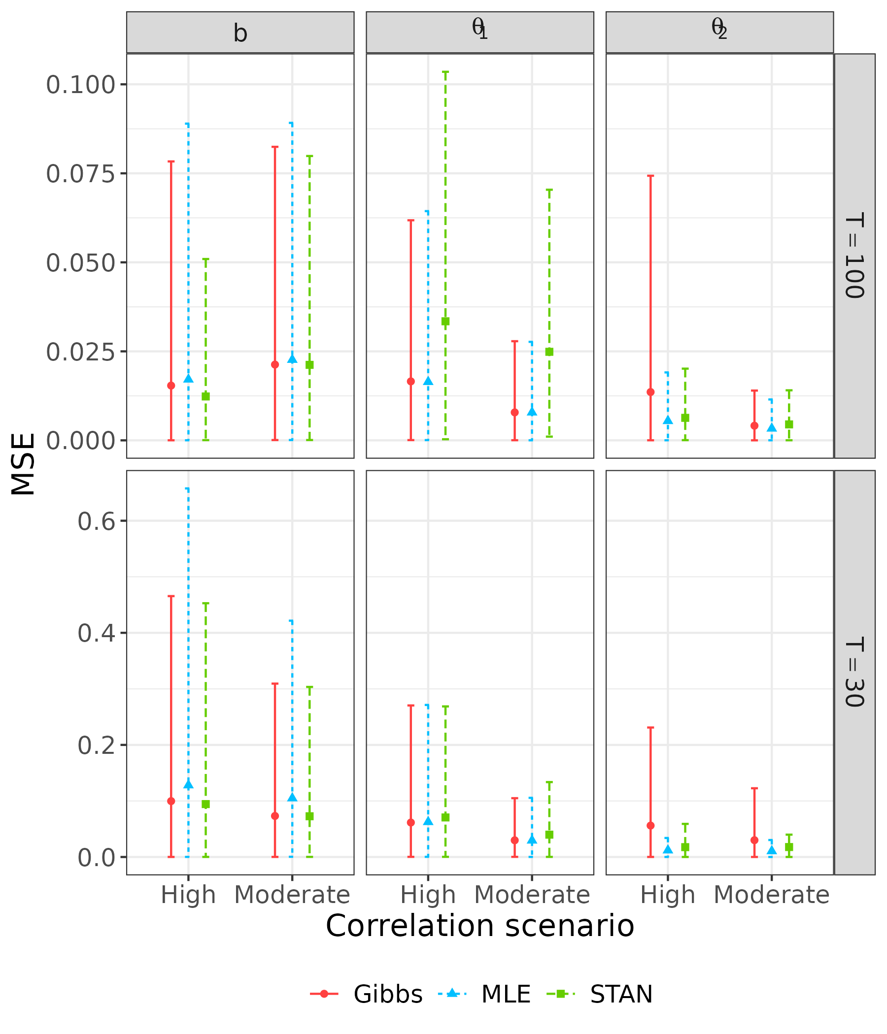
(a) MSE

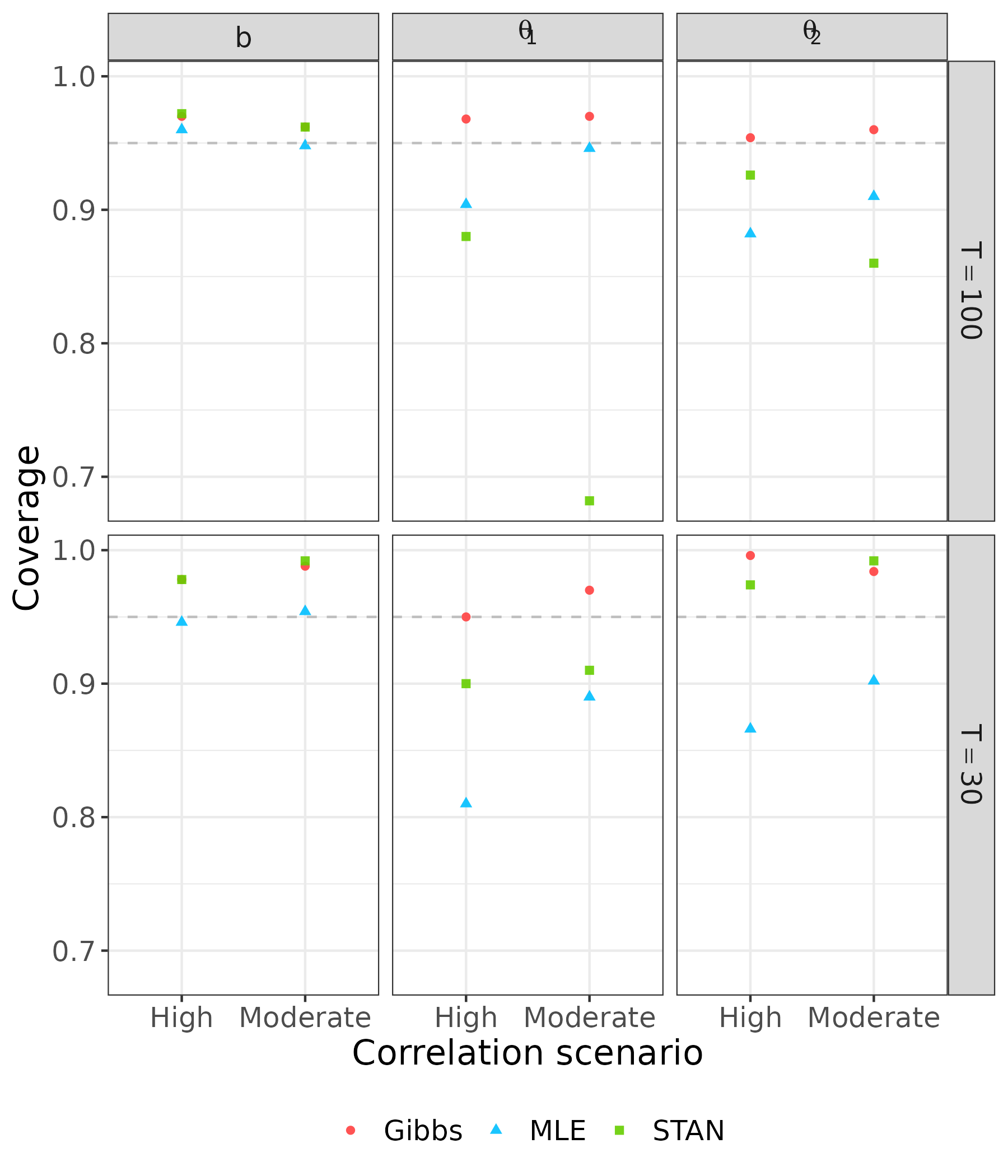
(b) Coverage

Figure 1: Results for the correctly specified model with Poisson distributed errors: Mean square error and $95\%$ coverage by correlation setting for each parameter and time series length $T$ for scenarios S1 - S4. Within each sub-figure, columns represent parameters and rows represent the different time series length $T$. Results form the Gibbs sampler are shown with points and solid lines results, results for the MLE approach are indicated by triangles and fine dashed lines, and results for STAN are displayed with squares and bold dashed lines. In the MSE plots (left panels), the central points/triangles indicate the mean values, and the error bars represent the 5th and 95th percentiles. The coverage plots (right panels) show the coverage obtained using credible intervals approximated from Gibbs samples (red points), STAN samples (green squares), and using Wald confidence intervals obtained using the MLE and is asymptotic variance produced by MCMC-EM.

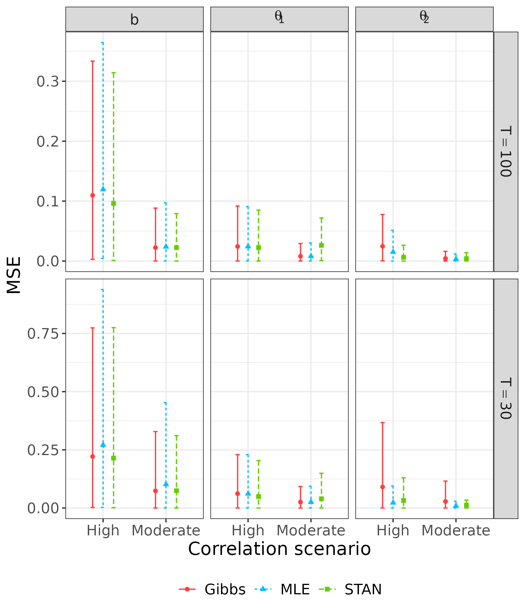
(a) MSE

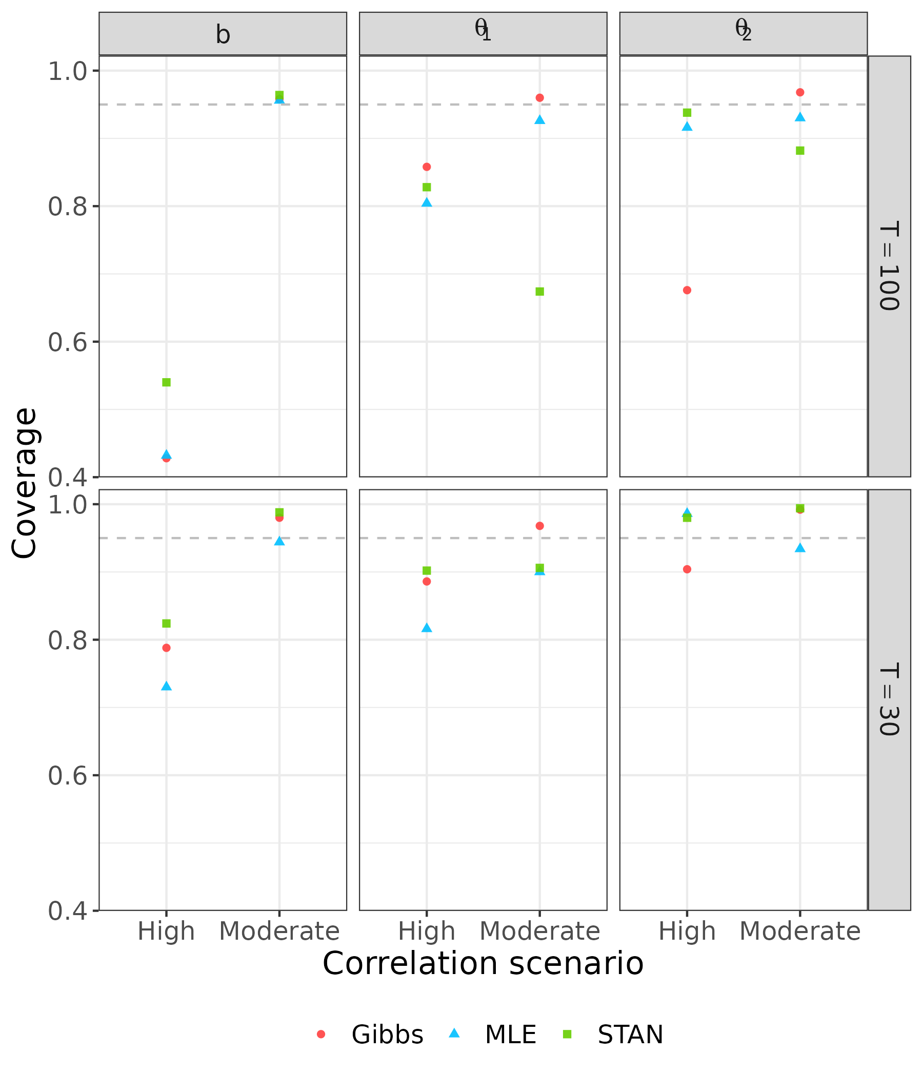
(b) Coverage

Figure 2: Results for the misspecified model with Negative binomial distributed errors: Mean square error and $95\%$ coverage by correlation scenario for each parameter and time series length $T$ for scenarios S5 - S8. Within each sub-figure, columns represent parameters and rows represent the different time series length $T$. Results form the Gibbs sampler are shown with points and solid lines results, results for the MLE approach are indicated by triangles and fine dashed lines, and results for STAN are displayed with squares and bold dashed lines. In the MSE plots (left panels), the central points/triangles indicate the mean values, and the error bars represent the 5th and 95th percentiles. The coverage plots (right panels) show the coverage obtained using credible intervals approximated from Gibbs samples (red points), STAN samples (green squares), and using Wald confidence intervals obtained using the MLE and is asymptotic variance produced by MCMC-EM.

5.1.2 Simulation results

As expected, the analysis based on the three algorithms improves as the time series length increases. Figure 1 presents the results for the correctly specified model with Poisson distributed errors. In most cases, the MSE values across the three inference methods are similar. The uncertainty is generally higher for the estimates of parameter $b$, lower for $\theta_{1}$, and even lower for $\theta_{2}$. An exception occurs with STAN when $T=100$, where the uncertainty for $\theta_{1}$ is greater than for $b$. Furthermore, for $\theta_{2}$, the Gibbs sampler produced estimates with greater uncertainty compared to the other two algorithms. In terms of coverage, all three inference methods yield values close to $0.95$ for the parameter $b$. However, the MLE approach shows lower coverage, particularly when $T=30$ and the correlation is high. This is likely due to the sample size being too small for the asymptotic variance estimate to be reliable. When $T=100$, the Gibbs sampler demonstrates the most accurate coverage across all parameters and correlation scenarios.

The results for the misspecified case are shown in Figure 2. In this setting, the performance of the algorithms differs noticeably between the high and moderate correlation scenarios. When the correlation is lower, the three algorithms exhibit improved performance, with lower MSE, reduced uncertainty, and more accurate coverage across all parameters and both sample sizes. Again, higher uncertainty is observed for the estimates of $b$ and $\theta_{1}$, and lower uncertainty for $\theta_{2}$. Moreover, when $T=100$, the Gibbs sampler provides the most accurate coverage for all parameters.

	1st Quantile	Mean	Median	3rd Quantile
Gibbs	1.33	1.33	1.33	1.34
MLE	9.21	11.82	11.23	13.38
STAN	6.98	7.66	7.09	7.31

Table 1: Summary statistics of the computational times (in minutes) under scenario S4

The computational times for scenario S4 are reported in Table 1. The MLE approach was the slowest, taking between two and nine times longer tan the other two. The Gibbs sampler outperforms STAN in terms of speed, with a mean computation time that is approximately five times shorter. The other scenarios exhibited similar patterns and are presented in the Supplementary Material. Finally, a comparison of the effective sample sizes for the three parameters across the two Bayesian inference methods is also provided there. In all cases, the Gibbs sampler outperformed STAN, yielding effective samples sizes per second that were around 1.5 to 3.5 times larger. This is of course not surprising, since the algorithm presented here has been designed specifically for this problem, while STAN is a sampling algorithm which is able to tackle a wide variety of models.

5.2 Real data analysis

We analyze here the American Redstart counts dataset which was previously discussed by Lele [2006] and Dennis et al. [2006]. This data set is recorded with the number 0214332808636 in the North American Breeding Bird Survey [Peterjohn, 1994, Robbins et al., 1986] and contains the number of specimens observed from 1966 to 1995 at a survey location. We fit the Gompertz model with Poisson-distributed errors to this dataset using both the Gibbs sampler and the MLE approach proposed here. STAN was also used as a baseline for comparison within the Bayesian framework.

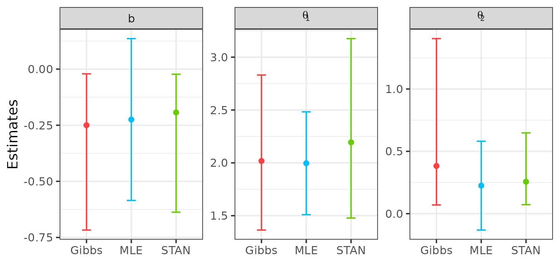
Figure 3: Point estimates for the three parameters obtained using each inference method. For the two Bayesian methods, the error bars represent the 95% credible intervals, while for the MLE, they indicate the Wald 95% confidence intervals .

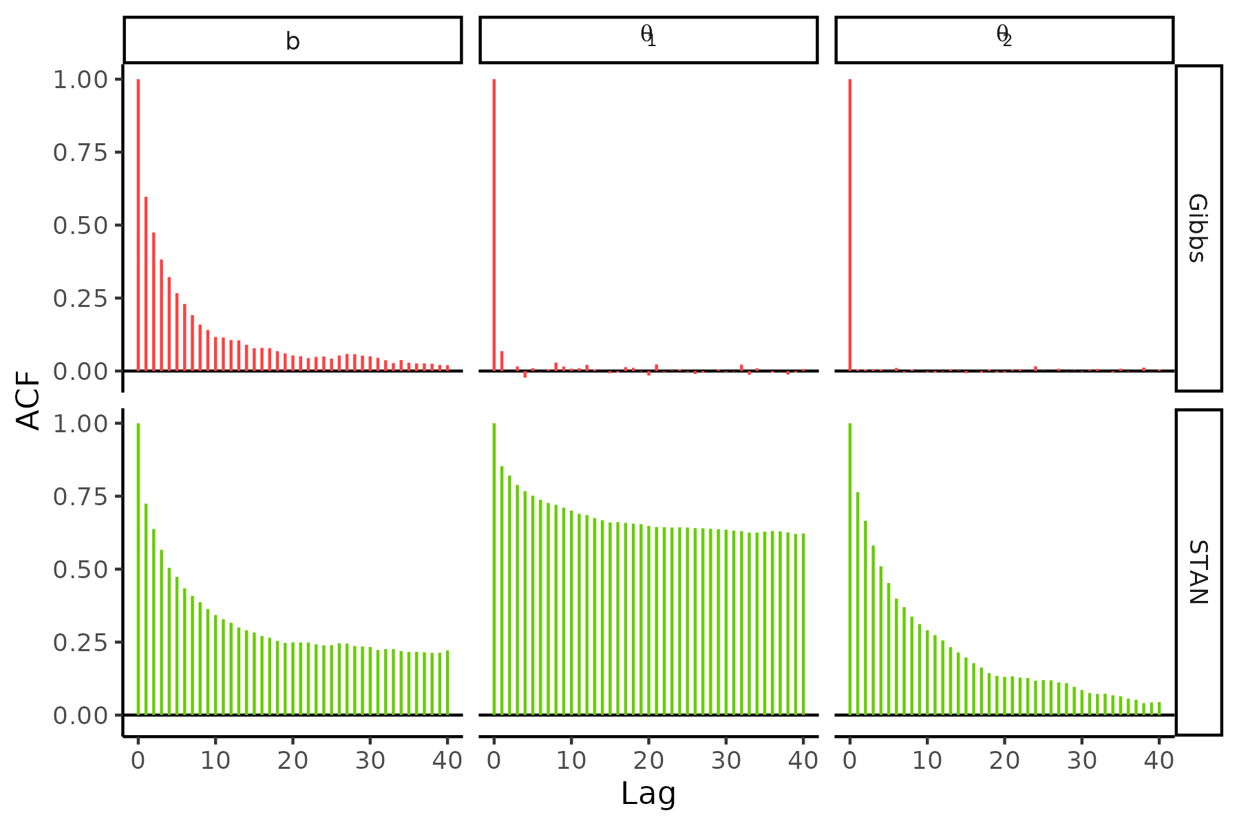
Figure 4: Autocorrelation functions of the posterior samples for the three parameters under both Bayesian inference methods.

We computed point estimates for the three parameters, along with the $95\%$ credible intervals for the Bayesian methods and the $95\%$ confidence intervals based on Gaussian approximation for the MLE approach (Figure 3). For the two Bayesian methods, we also calculated the effective sample size and autocorrelation function (Figure 4) for each parameter (Table 2).

Although the Gibbs sampler shows greater uncertainty in the estimation of $\theta_{2}$, the point estimates across the three methods remain comparable. However, when examining the effective sample size and autocorrelation functions of the posterior distributions for the two Bayesian methods, the Gibbs sampler demonstrates superior performance. The effective sample size for $\theta_{2}$ is nearly twice as large with the Gibbs sampler, six times larger for $b$, and increases for $\theta_{1}$, from only $30$ in STAN to more than $8200$ with the Gibbs sampler.

	b	$\theta_{1}$	$\theta_{2}$
Gibbs	1106.8	8239.5	10000
STAN	209.4	30.3	583.4

Table 2: Effective sample sizes for the three parameters from the analysis of the American Redstart for both Bayesian inference methods

6 Discussion

We develop full-likelihood-based inference within the frequentist and Bayesian paradigms for the Gompertz model with Poisson sampling errors. The proposed approaches remove the need to consider pseudo-likelihood methods that mitigate computational challenges at the price of reducing the information provided by the data.

In our future work, we would like to investigate whether similar developments can be produced to modified versions of the model considered here. The latter can be created by modifying the growth curve by adding parameters that allow curvature and long-term behavior [Asadi et al., 2023] or when the population dynamics is determined by a stochastic differential equation as in Donnet et al. [2010].

Code

The developed methods are available in a new R package: gse. The new R package and the scripts of Section 5 are available online on GitHub at the following link: https://github.com/sofiar/GMLossF

References

- Alexander et al. [2017] M. Alexander, E. Zagheni, and M. Barbieri. A flexible Bayesian model for estimating subnational mortality. Demography, 54(6):2025–2041, 2017.
- Asadi et al. [2023] M. Asadi, A. Di Crescenzo, F. A. Sajadi, and S. Spina. A generalized Gompertz growth model with applications and related birth-death processes. Ricerche di Matematica, 72(2):1–36, 2023.
- Auger-Méthé et al. [2021] M. Auger-Méthé, K. Newman, D. Cole, F. Empacher, R. Gryba, A. A. King, V. Leos-Barajas, J. Mills Flemming, A. Nielsen, G. Petris, and L. Thomas. A guide to state–space modeling of ecological time series. Ecological Monographs, 91(4):e01470, 2021.
- Baione and Levantesi [2018] F. Baione and S. Levantesi. Pricing critical illness insurance from prevalence rates: Gompertz versus Weibull. North American Actuarial Journal, 22(2):270–288, 2018.
- Booth and Hobert [1999] J. G. Booth and J. P. Hobert. Maximizing generalized linear mixed model likelihoods with an automated Monte Carlo EM algorithm. Journal of the Royal Statistical Society Series B: Statistical Methodology, 61(1):265–285, 1999.
- Butt and Haberman [2004] Z. Butt and S. Haberman. Application of frailty-based mortality models using generalized linear models. ASTIN Bulletin: The Journal of the IAA, 34(1):175–197, 2004.
- Caffo et al. [2005] B. Caffo, W. Jank, and G. Jones. Ascent-based Monte Carlo expectation–maximization. Journal of the Royal Statistical Society Series B: Statistical Methodology, 67(2):235–251, 2005.
- Chan and Ledolter [1995] K.-S. Chan and J. Ledolter. Monte Carlo EM estimation for time series models involving counts. Journal of the American Statistical Association, 90(429):242–252, 1995.
- Dempster et al. [1977] A. Dempster, N. Laird, and D. Rubin. Maximum likelihood from incomplete data via the EM algorithm. Journal of the royal statistical society: series B (methodological), 39(1):1–22, 1977.
- Dennis et al. [2006] B. Dennis, J. M. Ponciano, S. R. Lele, M. L. Taper, and D. F. Staples. Estimating density dependence, process noise, and observation error. Ecological Monographs, 76(3):323–341, 2006.
- Donnet et al. [2010] S. Donnet, J.-L. Foulley, and A. Samson. Bayesian analysis of growth curves using mixed models defined by stochastic differential equations. Biometrics, 66(3):733–741, 2010.
- Gompertz [1825] B. Gompertz. On the nature of the function expressive of the law of human mortality, and on a new mode of determining the value of life contingencies. In a letter to Francis Baily, Esq. FRS. Philosophical transactions of the Royal Society of London, (115):513–583, 1825.
- Hamilton [1994] J. Hamilton. Time Series Analysis. Princeton University Press, Princeton, NJ, 1994.
- Hostetler and Chandler [2015] J. A. Hostetler and R. B. Chandler. Improved state-space models for inference about spatial and temporal variation in abundance from count data. Ecology, 96(6):1713–1723, 2015.
- Lele [2006] S. R. Lele. Sampling variability and estimates of density dependence: A composite-likelihood approach. Ecology, 87(1):189–202, 2006.
- Lindén and Knape [2009] A. Lindén and J. Knape. Estimating environmental effects on population dynamics: consequences of observation error. Oikos, 118(5):675–680, 2009.
- Louis [1982] T. Louis. Finding the observed information matrix when using the EM algorithm. Journal of the Royal Statistical Society Series B: Statistical Methodology, 44(2):226–233, 1982.
- McCulloch [1994] C. E. McCulloch. Maximum likelihood variance components estimation for binary data. Journal of the American Statistical Association, 89(425):330–335, 1994.
- Newman et al. [2014] K. Newman, S. Buckland, B. Morgan, R. King, D. Borchers, D. Cole, P. Besbeas, O. Gimenez, and L. Thomas. Modelling Population Dynamics: Model Formulation, Fitting and Assessment using State-Space Methods. Springer, 2014.
- Peterjohn [1994] B. Peterjohn. The North American breeding bird survey. Birding, 26(6):386–398, 1994.
- Robbins et al. [1986] C. S. Robbins, D. Bystrak, and P. H. Geissler. The Breeding Bird Survey: its first fifteen years, 1965-1979. Technical report, US Fish and Wildlife Service, 1986.
- Staples et al. [2004] D. F. Staples, M. L. Taper, and B. Dennis. Estimating population trend and process variation for pva in the presence of sampling error. Ecology, 85(4):923–929, 2004.
- Tai and Noymer [2018] T. H. Tai and A. Noymer. Models for estimating empirical Gompertz mortality: With an application to evolution of the Gompertzian slope. Population Ecology, 60(1-2):171–184, 2018.
- Tjørve and Tjørve [2017] K. M. C. Tjørve and E. Tjørve. The use of Gompertz models in growth analyses, and new Gompertz-model approach: An addition to the unified-Richards family. PLOS ONE, 12(6):1–17, 06 2017.
- Wei and Tanner [1990] G. C. Wei and M. A. Tanner. A Monte Carlo implementation of the EM algorithm and the poor man’s data augmentation algorithms. Journal of the American statistical Association, 85(411):699–704, 1990.
- Winsor [1932] C. P. Winsor. The Gompertz curve as a growth curve. Proc Natl Acad Sci U S A, 18(1):1–8, Jan. 1932.