Precision measurement of the ¹⁷⁶Lu^{+ 3}D₁ microwave clock transitions

Abstract

We report precision measurement of the unperturbed ${{}^{3}}D_{1}$ microwave transition frequencies in ${}^{176}\mathrm{Lu}^{+}$ to a fractional uncertainty of $4\times 10^{-14}$. We find the $\ket{F,m_{F}}=\ket{8,0}$ to $\ket{7,0}$ hyperfine transition frequency to be $10\,491\,519\,945.228\,82(38)\,$Hz and the $\ket{7,0}$ to $\ket{6,0}$ transition frequency to be $11\,290\,004\,289.881\,61(36)\,$Hz. At this precision we are able to observe the hyperfine-mediated effects in the ratio of the quadrupole shifts, from which we can directly infer the residual quadrupole moment after ${}^{3}D_{1}$ hyperfine averaging. We find a residual quadrupole moment of ${-2.48(23)\times 10^{-4}}\,ea_{0}^{2}$, consistent with a previous assessment using a different and less direct method. With the unperturbed microwave frequencies accurately known, the residual quadrupole shift for a ${}^{176}\mathrm{Lu}^{+}$ (${}^{3}D_{1}$) optical frequency standard can henceforth be readily evaluated to $<10^{-20}$ uncertainty by routine ${{}^{3}}{D}_{1}$ microwave spectroscopy.

I Introduction

Optical and microwave frequency standards utilizing states with angular momentum $J>1/2$ have a quadrupole shift due to the coupling between the electronic quadrupole moment and electric field gradients. This is often a leading systematic shift in ion-based systems using strong electric field gradients for trapping [1, 2]. This shift is typically suppressed by some form of averaging, either over three orthogonal directions of the magnetic field orientation [3], over all magnetic substates [2], dynamic-decoupling [4], continuous rotation of magnetic field [5], or over hyperfine states $\ket{F,m=0}$ for all $F$ [6]. The ${}^{176}\mathrm{Lu}^{+}$ standard is so far unique in using hyperfine averaging (HA), which is realized either as an average of optical frequencies or, often more practically, as an equivalent linear combination of one optical and two microwave transition frequencies [7]. Although HA practically eliminates the leading quadrupole shift, a residual quadrupole moment (RQM) which arises from hyperfine-mediated mixing between fine-structure states remains [8, 9]. The quadrupole shift due to the RQM on the optical frequency is typically small, $<10^{-18}$, but must be assessed at the $10^{-19}$ level of systematic uncertainty now being reached [10]. The RQM for a ${}^{176}\mathrm{Lu}^{+}({{}^{3}}D_{1}$) frequency standard has been has estimated to be $-2.54\times 10^{-4}\,ea_{0}^{2}$  [8], where $e$ is the elementary electron charge and $a_{0}$ is the Bohr radius, but an effective means of measuring the electric field gradient in situ has been lacking.

The ${}^{176}\mathrm{Lu}^{+}$ ${{}^{3}}{D}_{1}$ microwave clock transition frequencies $\ket{F,m_{F}}=\ket{7,0}$ to $\ket{8,0}$ ($\ket{6,0}$), denoted $f_{1}$ ($f_{2}$) respectively, are routinely tracked with $\sim$mHz accuracy as part of ${}^{1}S_{0}$ to ${}^{3}{D}_{1}$ optical clock operation. The leading systematic shifts on these microwave transitions are the quadratic Zeeman shift and the quadrupole shift. The quadratic Zeeman shift is readily evaluated using the known quadratic Zeeman coefficients and the measured magnetic field amplitude inferred from the observed Zeeman splitting of $m=\pm 1$ magnetic field sensitive states. With accurate knowledge of the unperturbed microwave clock transition frequencies, the residual quadrupole shift on the HA optical clock frequency may be readily obtained from the quadrupole shifts on the microwave frequencies [11, 8].

Here we report precision measurement of the unperturbed ${}^{3}{D}_{1}$ microwave clock transition frequencies. First, the quadratic Zeeman coefficients are found by microwave Ramsey spectroscopy over a range of magnetic field amplitudes from 0.13 mT to 2.6 mT. The resulting quadratic Zeeman coefficients are consistent with previously reported values [10], but with one order of magnitude reduction in the uncertainty. We present a scheme to precisely set the orientation of the magnetic field using spectroscopic measurements on the ion. The orientation of the electric field gradient is characterized by measuring quadrupole shifts over a range of applied magnetic field directions. Finally, the unperturbed microwave transition frequencies are measured by averaging the quadrupole shift over three orthogonal directions of the magnetic field.

Applying the newly measured microwave frequencies, we demonstrated that for a large applied electric field gradient, the quadrupole shift can be evaluated with sufficient precision to resolve hyperfine-mediated effects. From the ratio of quadrupole shifts on the two microwave transitions, the RQM remaining after HA can be inferred, providing an independent experimental validation of the previously reported value derived from a combination of $g$-factor measurements and calculated matrix elements [10].

II Experimental system

Experiments are performed with a single ${}^{176}\mathrm{Lu}^{+}$ ion in the apparatus denoted ‘Lu-1’ in previous work [12]. The ion trap consists of two axial end caps separated by $\sim 2.7\,$mm and four rods arranged on a square with sides of 1.2 mm length. The rf potential at frequency $\Omega_{\mathrm{rf}}=2\pi\times 9.4\,$MHz is delivered via a quarter-wave helical resonator to two diagonally opposite rods. Under typical operating conditions, static potentials of 9 V are applied on the end caps and 0.5 V on the two other diagonally opposite rods, which, together with the rf-potential, results in measured trap frequencies for a single ${}^{176}\mathrm{Lu}^{+}$ion of $2\pi\times(648,614,177)$ kHz.

The atomic-level structure of ${}^{176}\mathrm{Lu}^{+}$ is shown in Fig. 1(a). Repump lasers at 350, 622, and 895 nm initialize population in the ${}^{3}D_{1}$ state. A laser at 646 nm provides Doppler cooling and state detection for the ${}^{3}D_{1}$ state by fluorescence collected onto a single photon counting module (SPCM). An additional $\pi$-polarized 646-nm beam addressing $F=7$ to $F^{\prime}=7$ facilitates state preparation into $\ket{{}^{3}D_{1},7,0}$. Lasers at 848 nm and 804 nm drive the ${}^{1}S_{0}$ to ${{}^{3}}D_{1}$ and ${}^{1}S_{0}$ to ${{}^{3}}D_{2}$ clock transitions, respectively. Two microwave antennas external to the vacuum chamber are used to drive the $\Delta m=0,\pm 1$ microwave transitions between hyperfine levels. The microwave polarization at the ion is coarsely controlled by manual repositioning of the antennas as required. Three orthogonal pairs of coils produce a magnetic field up to 0.2 mT at the ion, which can be oriented in any direction.

With the exception of auxiliary experiments to determine the magnetic field alignment, the primary measurements consist of Ramsey spectroscopy of the ${{}^{3}}D_{1}$ microwave clock transitions. For all measurements the interrogation sequence begins only after conditional detection of the ion in the ${{}^{3}}D_{1}$ state by fluorescence detection with repump and cooling beams on. The ion is then Doppler cooled for 5 ms and optically pumped for 1 ms to the $\ket{{}^{3}D_{1},7,0}$ state. Either the $\ket{7,0}$ to $\ket{8,0}$ or $\ket{7,0}$ to $\ket{6,0}$ microwave clock transition is interrogated by Ramsey spectroscopy with a typical $\frac{\pi}{2}$ pulse time of 5 ms and Ramsey time of $T=5\,$s if at low (0.1 mT) magnetic field. State detection of ${}^{3}D_{1}$ is performed after shelving $\ket{7,0}$ population to ${{}^{1}}S_{0}$ on the 848 nm optical clock transition.

A frequency discriminator is derived by alternately stepping the microwave frequency $\pm$ half of a Ramsey fringe and taking the difference. After averaging $N$ cycles, the microwave frequency is updated to track the center Ramsey fringe. We interleave additional microwave Rabi spectroscopy measurements to track the $\ket{{}^{3}D_{1},6,\pm 1}$ Zeeman splitting, which requires only a small fraction of the overall duty cycle. The magnetic field amplitude is inferred from the Zeeman splitting using the previously reported Landé g-factor [8].

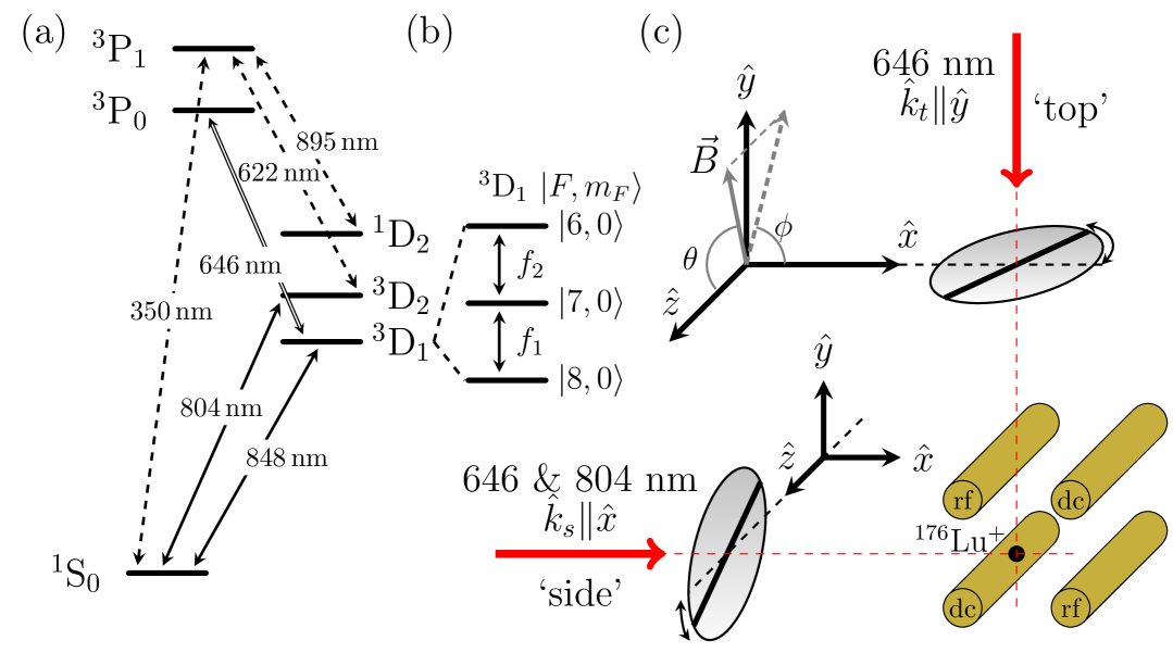
Figure 1: (a) Atomic-level structure of ¹⁷⁶Lu⁺ showing the wavelengths of repump (dashed lines), cooling/detection (double line), and clock (solid lines) transitions used. (b) Microwave clock transitions measured in this work. (c) Ion trap geometry with the orientation of lasers and polarizers used to precisely set the applied magnetic field direction as described in the main text.

III Theory

The quadrupole shift arises from coupling between the electric field gradient and electronic quadrupole moment of the atom [3]. In the principal-axis (primed) frame, the static electric potential in the neighborhood of the trapped ion has the simple form

$$\Phi(x^{\prime},y^{\prime},z^{\prime})=A[(x^{\prime 2}+y^{\prime 2}+z^{\prime 2})+\epsilon(x^{\prime 2}-y^{\prime 2})].$$ (1)

The quadrupole shift in the laboratory frame where the $z$ axis is aligned to the magnetic field is given by [3]

$$hf_{Q}(F,m_{F})=C_{F,m_{F}}\Theta(J)\\ \quad\times A[(3\cos^{2}{\beta}-1)-\epsilon\sin^{2}{\beta}(\cos^{2}\alpha-\sin^{2}\alpha)].$$ (2)

Here $\alpha$ and $\beta$ are the Euler angles for rotation of the principal axis frame to the laboratory frame following the conventions of [3],

$$C_{F,m_{F}}=(-1)^{2F-m_{F}+I+J}(2F+1)\begin{Bmatrix}F&2&F\\ J&I&J\end{Bmatrix}\\ \times\begin{pmatrix}F&2&F\\ -m_{F}&0&m_{F}\end{pmatrix}\begin{pmatrix}J&2&J\\ -J&0&J\end{pmatrix}^{-1},$$ (3)

and $\Theta(J)$ is the quadrupole moment for the fine-structure level defined by

$$\Theta(J)=\begin{pmatrix}J&2&J\\ -J&0&J\end{pmatrix}\langle J||\Theta^{(2)}||J\rangle.$$ (4)

The ¹⁷⁶Lu⁺ ${{}^{3}}{D}_{1}$ quadrupole moment has been previously reported as $\Theta(^{3}{D}_{1})=0.638\,62(74)\,ea_{0}^{2}$  [11]. The coefficients for quadrupole shift on the $f_{1}$ and $f_{2}$ microwave transitions are $C_{1}\equiv C_{7,0}-C_{8,0}=\frac{8}{5}$ and $C_{2}\equiv C_{6,0}-C_{7,0}=-\frac{7}{5}$, respectively. Neglecting stray dc gradients and the small rf contribution to the axial confinement, the gradient can be estimated by $A=-\frac{m\omega_{a}^{2}}{4e}$, where $m$ is the mass of the ion and $\omega_{a}=2\pi\times 177\,$kHz is axial confinement frequency for our typical applied dc voltages. The corresponding quadrupole shift is $\approx 0.78\,$Hz for the $f_{1}$ transition at the extremum when the magnetic field is aligned to the ion trap axis ($\beta=0$).

It is of interest to consider the ratio of the quadrupole shifts on the two microwave transitions, which would be precisely $r=\frac{C_{1}}{C_{2}}=-\frac{8}{7}$ in the absence of hyperfine mediated effects. Following the treatment in  [8], hyperfine mediated effects lead to a modified ratio

$$\tilde{r}=\frac{C_{1}\Theta(^{3}{D}_{1})-\frac{16}{175}\beta_{1,2}^{Q}}{C_{2}\Theta(^{3}{D}_{1})-\frac{3}{25}\beta_{1,2}^{Q}}\approx-1.146\,26(33)$$ (5)

where $\beta_{1,2}^{Q}=-0.0133(13)\,ea_{0}^{2}$ is the dominant RQM correction due to mixing with the ${{}^{3}}D_{2}$ state reported in [8]. The uncertainty of $\beta_{1,2}^{Q}$ is estimated to be $10\%$ limited by theory. Experimental determination of the ratio with $\sim 0.03\%$ uncertainty would provide direct experimental validation of the residual quadrupole shift assessment which in [8] has been determined from a combination of $g$-factor measurements and theory.

IV Calibration of Magnetic Field Alignment

The quadrupole shift averaged over any three mutually orthogonal directions is zero [3]. An essential part of this work is to precisely calibrate the angular orientation of the magnetic field, given by the spherical coordinates $(\theta,\phi)$ in the laboratory frame $($x,y,z$)$, as illustrated in Fig. 1c. The key technique is to use measurements on the ion to always align the magnetic field to the linear polarization of a nominally $\pi$-polarized 646-nm laser used for optical pumping (OP) which provides a precise reference in the laboratory frame. As shown in Fig. 1c, the wave vector $\hat{k}_{t}$ of the OP laser from the ’top’ defines the $\hat{y}$ axis and by rotating the angle of the ‘top’ linear polarizer, the magnetic field $\vec{B}$ can be set to any angle $\theta$ in the $xz$-plane $(\phi=0)$ by aligning to the laser polarization. By sending the OP laser from the side, $\hat{k_{s}}=\hat{x}$, we can set $\vec{B}$ to any angle $\theta$ in the $yz$-plane $(\phi=\frac{\pi}{2})$ referenced by the rotation angle of the ‘side’ polarizer. We ensure that $\hat{k}_{s}\parallel\hat{x}$ by auxiliary measurements on the ion making use of the selection rules for the electric quadrupole (E2) transition at 804-nm.

First we describe the procedure to align the magnetic field to the linear polarization of a $\pi$-polarized 646-nm OP laser. This is done by scanning the angular deflection of the magnetic field and observing the depumping rate out of the $\ket{{}^{3}D_{1},7,0}$ state from the OP laser due to small angle misalignment of the magnetic field relative to the laser polarization. The depumping rate is measured by first preparing in $\ket{{}^{3}D_{1},7,0}$, pulsing on only the 646-nm OP beam addressing $F=7$ to $F^{\prime}=7$ for a fixed duration, shelving the remaining $\ket{{}^{3}D_{1},7,0}$ population to $\ket{{}^{1}S_{0},7,0}$ with the 848-nm clock laser, and finally state detection of $\ket{{}^{3}D_{1}}$. Fig. 2(a) shows the observed population for a typical scan of the magnetic field deflection. The typical fit uncertainty is 0.05^∘, and repeated scans yield optimum values consistent with this uncertainty. Small angle scans are performed in both $\theta$ and $\phi$ to optimize alignment of the magnetic field to the 646-nm laser polarization.

The laboratory coordinates axes ($x$,$y$,$z$) are defined by the OP laser labeled ‘top’ as shown in Fig. 1c. The optics assembly is rigidly attached to the vacuum chamber with the laser light delivered by optical fiber. The light is collimated and passed through a high extinction ratio ($>10^{5}$) linear film polarizer in a precision rotation mount before being focused onto the ion by a lens. The rotation mount has a vernier scale by which the rotation angle can be reliably set with 5 arcmin precision. The $\hat{y}$ axis is defined as the propagation direction $\hat{k_{t}}$, the $\hat{z}$ axis by the polarization of the OP laser when the polarizer is set to a reference angle approximately aligned to the ion trap axis, and the $\hat{x}$ axis as the polarization of the OP laser with the polarizer rotated $90^{\circ}$ with respect to the $\hat{z}$ setting. By setting the polarizer angle and then aligning the magnetic field to the OP laser polarization, we are then able to precisely set the magnetic field to any direction in the $xz$-plane. We bound systematic uncertainty by rotating the polarizer by 180^∘ and repeating the magnetic field alignment, for which we find a difference of 0.4^∘ in the re-optimized field direction. We take this as the systematic uncertainty in the orthogonality of $\hat{x}$ and $\hat{z}$ magnetic field settings.

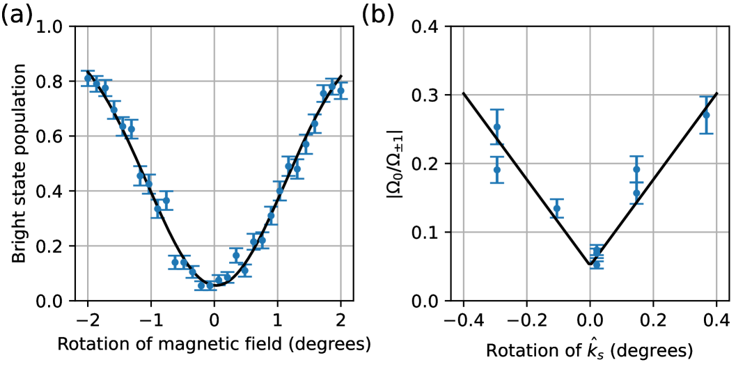
Figure 2: (a) Example of alignment of the magnetic field to the linear OP polarization. (b) Example of alignment of $\hat{k}_{s}$ to the magnetic field via the 804-nm transition E2 coupling.

To access a third orthogonal direction, we require an additional 646 nm OP laser from another direction, labelled ‘side’ in Fig. 1c. Here we describe the procedure to ensure the propagation direction of the laser, $\hat{k_{s}}$, is well aligned in the coordinate frame defined by the ‘top’ beam. For the ‘side’ optics assembly, both 646 nm and 804 nm light are delivered over the same optical fiber and the entire assembly is on a tip/tilt stage. Again a linear film polarizer in a precision rotation mount determines the polarization. We use the relative coupling strengths $\Omega_{\Delta m}$ for $\Delta m=[0,\pm 1]$ on the E2 clock transitions at 804 nm to align $\hat{k}_{s}$ to $\hat{x}$ by minimizing the ratio $\left|\frac{\Omega_{0}}{\Omega_{\pm 1}}\right|$ via the tip/tilt stage. With $\vec{B}$ aligned to $\hat{x}$, the 804 nm laser polarization is set to $\hat{y}$ ($\hat{z}$) and the the rotation of $\hat{k}_{s}$ about $\hat{z}$ ($\hat{y}$) is adjusted to find the minimum ratio, as shown in Fig. 2(b) for one of the rotation directions. Next, with $\vec{B}$ aligned to $\hat{z}$ as referenced from the ‘top’, we find the rotation angle of the ‘side’ polarizer that minimizes 646-nm depumping. A 90^∘ rotation of the polarizer from this position sets the ‘side’ OP laser polarization to $\hat{y}$. As a final consistency check, we compare the alignment of $\vec{B}$ when set to $\hat{z}$ referenced from either the ‘top’ or ‘side’ OP laser. These two methods agree to within $0.5^{\circ}$, which we take as systematic uncertainty in the coincidence of the ‘side’ reference frame relative to the ‘top’ reference frame.

To summarize, by referencing the magnetic field to the OP laser polarization from either the ‘top’ or ‘side’, we are able to precisely set the field direction in the laboratory frame spherical coordinates $(\theta,\phi)$ shown Fig. 1 to any $\theta$ where $\phi$ is restricted to 0 or $\frac{\pi}{2}$, when referenced from the ‘top’ or ‘side’ ports respectively. The systematic uncertainty in the orthogonality of $\hat{x}$, $\hat{y}$, and $\hat{z}$ magnetic field orientations is estimated to be $0.5^{{}^{\circ}}$.

V Measurement of quadratic Zeeman coefficients

Measured values for quadratic Zeeman coefficients of the ${{}^{3}}D_{1}$ microwave transitions, $\alpha_{1}$ and $\alpha_{2}$, were previously reported in the supplemental material of  [10]. Here we remeasure these coefficients with improved precision. Measurements of both $f_{1}$ and $f_{2}$ are taken at magnetic field amplitudes near 0.13, 0.8 and 2.6 mT with Ramsey interrogation times of 8 s, 1 s, and 250 ms, respectively. Short time scale magnetic field noise of $\sim 10$ nT limits the Ramsey coherence time at larger magnetic fields due to the increased linear sensitivity, $\frac{df_{i}}{dB}=2\alpha_{i}B$ for the transitions $i={1,2}$. For magnetic fields $>$0.13 mT, neodymium permanent magnets external to the experiment chamber provide additional bias while the coil pairs provide fine control of the magnetic field orientation and amplitude. For all measurements to determine the quadratic Zeeman coefficients the magnetic field is aligned to the OP laser reference with the polarizer position at a fixed angle throughout, corresponding to $(\theta,\phi)\approx(54^{\circ},0)$. This is the standard orientation used for clock operation in our lab, although in retrospect $\theta=0$ would have been advantageous for this measurement.

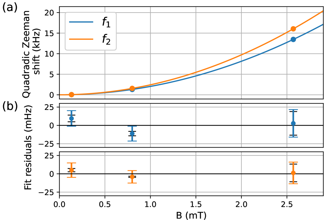
Figure 3: Evaluation of microwave quadratic Zeeman coefficients. (a) Measurements of both ${{}^{3}}D_{1}$ microwave transitions measured as a function of magnetic field amplitude. Solid lines are a quadratic fit. (b) Residuals with respect to the fit. The larger error bars are the combined total uncertainty, and the black error bars are the statistical component only.

Results are shown in Fig. 3(a) where each point represents the mean from several hours of averaging. The quadratic Zeeman coefficients are determined from a quadratic fit after subtracting the quartic component, $\lambda_{i}B^{4}$, where the coefficients $\lambda_{1}=-146\,\mu\mathrm{Hz}/\mathrm{mT}^{4}$ and $\lambda_{2}=-311\,\mu\mathrm{Hz}/\mathrm{mT}^{4}$ are evaluated from perturbation theory. The quartic component corrects the highest field measurements at the level of 1$\sigma$. The total and statistical uncertainties for each measurement can be seen in the fit residuals shown in Fig. 3(b). The dominant systematic is the uncertainty in the quadrupole shift when repeating the alignment of the magnetic field between configurations. We expect $\theta\approx 54^{\circ}$ is near to the angle $\beta=1/\sqrt{3}$ where the quadrupole shift, Eq. (2), vanishes but has linear sensitivity to variation in the angle. We estimate $\pm 0.5^{\circ}$ reproducibility of the field alignment for the high field measurements which contributes 10 mHz uncertainty through the quadrupole shift. Other systemics are estimated to be $<1$ mHz and detailed in the following section.

We find the quadratic Zeeman coefficients

$$\alpha_{1} =2\,038.589\,1(31)~\mathrm{Hz}\,\mathrm{mT}^{-2}~\mathrm{and,}$$

$$\alpha_{2} =2\,428.947\,0(26)~\mathrm{Hz}\,\mathrm{mT}^{-2}\mathrm{.}$$

The uncertainties are reduced by $\sim 14$ times compared to the previously reported values [10], and both are consistent to within $<$1.3$\sigma$ of the previous larger uncertainties.

VI Quadrupole Shift Evaluation and Microwave Frequency Measurement

We first determine the orientation of the electric field gradient by measuring the microwave frequency $f_{1}$ with the applied magnetic field oriented over the range of $(\theta,\phi)$ accessible by our alignment procedure. All measurements are carried out at a magnetic field near 0.1 mT and with Ramsey interrogation time of $5-10\,$s. Results are shown in Fig. 4 for both the typical applied dc bias voltage and for no dc bias voltages. Approximately 0.5 h of data collection was taken for each data point in order to average down to a statistical uncertainty of $\sim 2$ mHz. The quadratic Zeeman shift is evaluated from the magnetic field inferred from interleaved measurements and has been subtracted from the data. Other systematic shifts are $<1$ mHz.

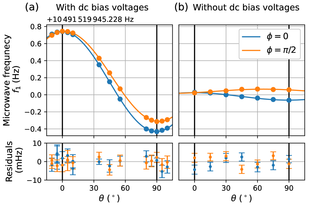
Figure 4: Measurements of the ${{}^{3}}D_{1}$ $\ket{7,0}$ to $\ket{8,0}$ transition for a range of magnetic field orientations $(\theta,\phi)$ for (a) the typical applied dc biases, and (b) no applied dc bias. Solid lines are the fit to the quadrupole shift model given Eq. (2). The reduced $\chi^{2}$ is $0.93$ with 25 degrees of freedom and 1.5 with 8 degrees of freedom for (a) and (b) respectively. Fit residuals are shown in the bottom plots.

In order to model the data by Eq. (2), we allow for an arbitrary rotation $R(\theta_{x},\theta_{y},\theta_{z})=X_{\theta_{x}}Y_{\theta_{y}}Z_{\theta_{z}}$ which brings the magnetic field coordinates from the laboratory frame to the principal-axis frame, in effect mapping the coordinates $(\theta,\phi)$ to $(\beta,\alpha)$. From numerical simulation of the ion trap with typical dc voltages applied, we would expect $(\theta_{x},\theta_{y},\theta_{z})\approx(0,0,\frac{\pi}{4})$, and $A\approx-53\,\mathrm{V}/\mathrm{cm}^{2}$, $\epsilon\approx 0.7$, if the stray gradients are negligible [13, 2]. The fit for this case is shown in Fig. 4a and is in close agreement with fit parameters $[\theta_{x},\theta_{y},\theta_{z}]$ $=$ $[1.7(1)^{\circ},1.1(1)^{\circ},39(2)^{\circ}]$, $A=-53.77(5)\,\mathrm{V}/\mathrm{cm}^{2}$, $\epsilon=0.71(0.20)$.

In order to determine the unperturbed microwave frequencies with the highest possible accuracy, we reduce the amplitude of the quadrupole shift by removing applied dc gradients. No dc offset bias are applied to electrode pairs with only differential dc voltages applied as necessary to compensation micromotion. The rf drive is also increased such that we obtain trap frequencies $2\pi\times(1190,1100,95)\,$ kHz from only the rf field confinement and any stray dc gradients. As shown by the fit in Fig. 4b, this reduces the amplitude of the quadrupole shift by one order of magnitude, but with principal axis no longer closely aligned to the trap orientation.

We determine the unperturbed absolute frequencies $f_{1}$ and $f_{2}$ by taking the average of measurements in the three orthogonal directions $(\hat{x},\hat{y},\hat{z})$ for the configuration with no applied bias voltages. For each orientation, $f_{1}$ and $f_{2}$ are measured in an interleave for approximately 5 hours each in order to average down to a statistical uncertainty of $0.5\,$mHz per measurement. We find the unperturbed microwave transition frequencies to be

$$f_{1} =10\,491\,519\,945.228\,{82\pm(32)_{\mathrm{stat}}\pm(23)_{\mathrm{sys}}}\,\mathrm{Hz},~\mathrm{and}$$

$$f_{2} =11\,290\,004\,289.881\,{61\pm(32)_{\mathrm{stat}}\pm(20)_{\mathrm{sys}}}\,\mathrm{Hz}.$$

The systematic effects and uncertainties are summarized in Table 1. The systematics are evaluated to be less than the statistical uncertainty. The leading systematics are excess micromotion (EMM) and incomplete cancellation of quadrupole shift due to the systematic uncertainty in the orthogonality of the three magnetic field orientations. The orientation of the principal axis frame as determined by the quadruple model fit shown in Fig. 4b is used to evaluate the sensitivity to systematic errors in axes orientations. The quadrupole averaging uncertainty given in Table 1 is estimated by Monte Carlo sampling allowing for 0.5^∘ systematic uncertainty in the orthogonality of the measurement axes.

Table 1: Systematic corrections and uncertainties for the absolute frequency measurement ${}^{176}\mathrm{Lu}^{+}$ ${{}^{3}}D_{1}$ microwave clock transitions $\ket{7,0}$ to $\ket{8,0}$ ($f_{1}$) and $\ket{7,0}$ to $\ket{6,0}$ ($f_{2}$). All offsets and uncertainties are given fractionally at $10^{-14}$ relative to the respective frequencies. $\dagger$ Quadratic Zeeman shifts are corrected point by point from interleaved field measurements.

	$f_{1}$		$f_{2}$
Systematic	Corr.	Unc.	Corr.	Unc.
Quadrupole averaging	0.0	1.3	0.0	1.1
Micromotion	0.0	1.7	0.0	1.4
Maser calibration	-1.3	0.5	-1.3	0.5
Microwave ac Zeeman	-0.1	0.1	-0.1	$0.2$
Quadratic Zeeman	$\dagger\,\,$	0.3	$\dagger\,\,$	0.2
$B$ field evaluation	0.9	$<0.1$	1.0	$<0.1$
rf ac Zeeman	1.3	0.1	1.2	0.1
Total	0.8	2.2	0.8	1.9

The contribution from excess micromotion (EMM) relevant to the microwave transitions is the tensor component of the ac Stark shift. The shift on the microwave transition frequency, $\Delta f_{i}$, may be written [14]

$$\Delta f_{i}=-\frac{1}{4h}\Delta\alpha^{(2)}_{i}\left(\frac{m\Omega_{\mathrm{rf}}}{e}\right)^{2}\langle v^{2}\rangle(3\cos^{2}{\zeta}-1),$$ (6)

where $v$ is the velocity of the ion due to EMM, $\zeta$ is the angle between the applied magnetic field and the direction of rf field at the ion, and $\Delta\alpha^{(2)}_{i}$ is the differential tensor polarizability. The differential tensor polarizability on the $f_{1}$ transition, for example, is given by $\Delta\alpha^{(2)}_{1}=(C_{7,0}-C_{8,0})\alpha^{(2)}$, where $\alpha^{(2)}=-4.40(34)$, in atomic units, is the dc tensor polarizability of the ${}^{3}D_{1}$ term [15] and the coefficients are as given by Eq. (3). EMM is measured in three orthogonal directions using phase modulated sideband spectroscopy on the ${}^{1}S_{0}$ to ${}^{3}D_{2}$ optical clock transition [12]. EMM was compensated before and after each microwave measurement in the three orthogonal directions $(\hat{x},\hat{y},\hat{z})$, to the level of $|\frac{\Delta f_{i}}{f_{i}}|\lesssim\times 1\times 10^{-16}$ evaluated for the extreme ($\zeta=0$) field orientation. Just as for the quadrupole shift, the EMM tensor shift averaged over any three orthogonal directions is zero. However, variations in the amplitude or direction of the EMM during the microwave measurement campaign may result in a non-zero average. As the EMM compensation was not continuously monitored during the microwave spectroscopy, we take the full magnitude of the increase in EMM after each measurement as the systematic uncertainty of the EMM shift on each of the microwave frequencies.

The microwave synthesizers are referenced to a hydrogen maser and have $\sim 1$ $\mu$Hz resolution in the frequency setting. The hydrogen maser frequency is evaluated with respect to the Lu⁺ (${}^{3}D_{1}$) optical frequency standard [16] before and after microwave frequency measurements. The interpolated fractional frequency offset of the maser is evaluated to be $-1.3(0.5)\times 10^{-14}$ over the duration of the microwave measurements.

The microwave fields used for Ramsey spectroscopy contribute an ac-Zeeman shift. The frequency shift is largely suppressed by the long (5 s) Ramsey time compared to the short ($\sim$5 ms) $\frac{\pi}{2}$ pulse time. For some measurements the shift is as large as 100 $\mu$Hz when the microwave polarization is particularly imbalanced. Each time the magnetic field orientation was changed, the microwave field polarization was reevaluated by comparing the coupling strength on $m_{F}=0$ to $m_{F}^{\prime}=[-1,0,1]$ microwave transitions. Expressions for evaluation of the probe-induced microwave ac-Zeeman shift are given in the Supplemental Material of  [10].

The quadratic Zeeman coefficients $\alpha_{i}$ reported in Sec. VI contribute $\sim 3\times 10^{-15}$ fractional uncertainty at a 0.1 mT magnetic field. The magnetic field is inferred from the Zeeman splitting of the $\ket{6,\pm 1}$ states as measured by Rabi spectroscopy on the $\ket{7,0}$ to $\ket{6,\pm 1}$ microwave transitions on interleaved measurements. An imbalance in the $\sigma^{\pm}$ polarization components or a relatively large $\pi$ component of this microwave field gives rise to a differential ac Zeeman shift on these lines and consequently an error, $\delta B$, in the inferred magnetic field. Detailed calculations on the determination of $\delta B$ are given in Appendix A. The systematic shift on the microwave clock transition frequency is $\approx 2\alpha_{i}B\delta B$ and $\lesssim 100\,\mu$Hz.

Electric currents to the trap electrodes driven by the rf-trapping potential give rise to an rf-magnetic field and corresponding ac-Zeeman shift. The shift depends on the component of the rf-field perpendicular to the applied dc field [17]. We determine both the amplitude and orientation of the rf-magnetic field by measuring the Autler-Townes splitting on the Ba⁺ clock transition [18] for the applied magnetic field in each of the three orthogonal directions. We determine the rf magnetic field component amplitudes to be

$$[B_{x},B_{y},B_{z}]=[0.461(14),0.3081(93),0.2216(66)]\,\mu\mathrm{T}.$$

The systematic shift on the microwave clock transition is $\sim 200\,\mu$Hz for all three measurement orientations.

The rf electric field gradients used to trap the ion also give rise to a second-order ac-quadrupole shift, which does not average to zero over three mutually orthogonal magnetic field orientations [19]. This shift is evaluated to be $<2\times 10^{-16}$ fractionally and so is not included in Table 1.

VII Hyperfine mediated effects

As motivated in Sec. III, we consider the ratio of quadrupole shifts on transitions $f_{1}$ and $f_{2}$. Fig. 5(a,c) shows the quadrupole shifts and ratios in the three directions from the frequency measurement data where no bias voltages were applied. Here the quadrupole shifts are small, so the fractional uncertainty in ratio is large compared to the hyperfine mediated effects. The ratios are statistically consistent for all three orientations suggesting there is no orientation dependent systematic unaccounted for. To increase the precision on the ratio measurement, we apply a high bias voltage of 38 V on the endcap electrodes which gives an axial trapping frequency of 370 kHz. From 22 hours of measurement time with the magnetic field aligned to the trap axis, we find the quadrupole shifts and ratio shown in Fig. 5(b,d).

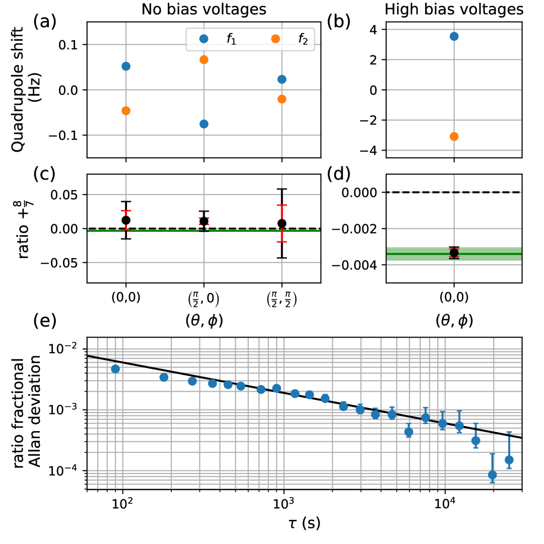
Figure 5: (a,b) Quadrupole shifts measured with no bias applied (a) and with high bias applied (b). Error bars are smaller than the points. (c,d) measured ratio of quadruple shift compared to the expected value (green line) based on the evaluation hyperfine mediated effects in [8] (Eq. (5)). (e) Allan deviation of ratio measurement at high bias.

The deviation from $-\frac{8}{7}$ is clearly observed and from Eq. (5) we can directly infer

$$\beta_{1,2}^{Q}=[-{0.01304}\pm(91)_{\mathrm{stat}}\pm(85)_{\mathrm{sys}}]ea_{0}^{2}$$ (7)

consistent with the value reported in  [8]. This measurement provides a fully experimental verification of the assessment of the RQM given in  [8] with a comparable level of uncertainty:

$$\langle\delta\Theta\rangle_{F}\approx\frac{2}{105}\beta_{1,2}^{Q}=[{-2.48}\pm(17)_{\mathrm{stat}}\pm(16)_{\mathrm{sys}}]\times 10^{-4}ea_{0}^{2}.$$ (8)

VIII Discussion

In summary we have measured both ${}^{176}\mathrm{Lu}^{+}$ ${}^{3}D_{1}$ microwave transition frequencies to fractional accuracy of $4\times 10^{-14}$. Although the motivation for this work was not to develop a microwave frequency standard, for comparison we note that the fractional frequency accuracy is only a factor of two to four worse than the highest accuracies reported for frequency standards based on the microwave transitions in trapped ion systems, including Cd⁺ [20], Hg⁺ [21], and Yb⁺ [22].

The unperturbed microwave frequencies measured here enable measurement of the ${}^{3}D_{1}$ microwave quadrupole shifts, providing a simple and accurate means to evaluation the residual quadrupole shift in ${}^{176}\mathrm{Lu}^{+}$ (${}^{3}D_{1}$) optical frequency standards.

We extend this application to measurement of the ratio of quadrupole shift with sufficient precision to infer the RQM resulting from hyperfine mediated effects. The inferred RQM is in agreement with the previous evaluation [8]. Consistency in results from the two different approaches provide greater confidence in the RQM assessment for ${}^{176}\mathrm{Lu}^{+}$ (${}^{3}D_{1}$) optical frequency standards.

Appendix A Field determination error

Given that the quadratic Zeeman shift is the largest shift on the microwave clock frequency, any errors in the determination of the magnetic field through the Zeeman servo can lead to shifts $\sim 100\,\mu$Hz. There is a bias in the magnetic field assessment depending on the polarization of the microwave field. We adopt the notation $a_{k,q}$ to refer to the $q$ polarization component of the horn driving the microwave transition $k$, where $\sum_{q}a_{k,q}^{2}=1$. The microwave polarizations are determined by ratios of pi-times on the $\pi,\sigma_{\pm}$ transitions.

$$\frac{a_{1\pm}}{a_{10}}=\frac{4}{3}\frac{\tau_{10}}{\tau_{1\pm}}\qquad\frac{a_{2\pm}}{a_{20}}=\sqrt{\frac{7}{3}}\frac{\tau_{20}}{\tau_{2\pm}}$$ (9)

When probing the Zeeman pair $\ket{7,0}$ to $\ket{6,\pm 1}$ to determine the magnetic field, there is a probe-induced shift due to off-resonant coupling primarily from $\ket{6,\pm 1}$ to $\ket{7,\pm 1}$, but also $\ket{6,\pm 1}$ to $\ket{7,\pm 2}$ and $\ket{7,0}$ to $\ket{6,0}$. The shifts on each level are given as follows

$$\Delta_{7,0}^{(\pm)} =\mp\frac{(\Omega_{7060})^{2}}{4\omega_{6}}\mp\frac{(\Omega_{706(\mp 1)})^{2}}{4(2\omega_{6})}$$

$$=\mp\frac{(\Omega_{7060})^{2}}{4\omega_{6}}\left(1+\frac{3}{14}\left(\frac{a_{2\mp}}{a_{20}}\right)^{2}\right)$$ (10)

$$\Delta_{6,\pm 1}^{(\pm)} =\mp\frac{(\Omega_{7(\pm 1)6(\pm 1)})^{2}}{4\omega_{7}}\mp\frac{(\Omega_{7(\pm 2)6(\pm 1)})^{2}}{4(2\omega_{7})}$$

$$=\mp\frac{(\Omega_{7060})^{2}}{4\omega_{7}}\left(\frac{48}{49}+\frac{18}{49}\left(\frac{a_{2\mp}}{a_{20}}\right)^{2}\right)$$ (11)

where $\hbar\omega_{F}=|g_{F}\mu_{B}B|$ are the Zeeman splittings and $\Omega_{FmF^{\prime}m^{\prime}}$ is the coupling from $\ket{F,m}$ to $\ket{F^{\prime},m^{\prime}}$. The overall shift when probing the $\ket{7,0}$ to $\ket{6,\pm 1}$ transition is given by $\Delta_{6,1_{\pm}}^{(\pm)}-\Delta_{7,0}^{(\pm)}$. The shift in the linear Zeeman splitting and the magnetic field are given as follows

$$\delta B=\frac{\hbar}{\mu_{B}g_{6}}\Delta\omega_{6}=\hbar\frac{(\Delta_{6,+1}^{(+)}-\Delta_{7,0}^{(+)})-(\Delta_{6,1_{-}}^{(-)}-\Delta_{7,0}^{(-)})}{2\mu_{B}g_{6}}.$$

The systematic shift on the microwave clock transition frequency is

$$\Delta f_{k}=\alpha_{k}(B+\delta B)^{2}-\alpha_{k}B^{2}\approx 2\alpha_{k}B\delta B.$$

Similarly we have the following expressions when probing the $\ket{7,0}$ to $\ket{8,\pm 1}$ Zeeman pair to determine the magnetic field:

$$\Delta_{7,0}^{(\pm)} =\mp\frac{(\Omega_{7080})^{2}}{4\omega_{8}}\mp\frac{(\Omega_{708(\mp 1)})^{2}}{4(2\omega_{8})}$$

$$=\mp\frac{(\Omega_{7080})^{2}}{4\omega_{8}}\left(1+\frac{9}{32}\left(\frac{a_{1\mp}}{a_{10}}\right)^{2}\right)$$ (12)

$$\Delta_{8,\pm 1}^{(\pm)} =\mp\frac{(\Omega_{7(\pm 1)8(\pm 1)})^{2}}{4\omega_{7}}\mp\frac{(\Omega_{7(\pm 2)8(\pm 1)})^{2}}{4(2\omega_{7})}$$

$$=\mp\frac{(\Omega_{7080})^{2}}{4\omega_{7}}\left(\frac{63}{64}+\frac{21}{128}\left(\frac{a_{1\mp}}{a_{10}}\right)^{2}\right).$$ (13)

For this case, the shift in the linear Zeeman splitting is

$$\delta B=\frac{\hbar}{\mu_{B}g_{8}}\Delta\omega_{8}=\hbar\frac{(\Delta_{8,+1}^{(+)}-\Delta_{8,0}^{(+)})-(\Delta_{8,-1}^{(-)}-\Delta_{8,0}^{(-)})}{2\mu_{B}g_{8}}.$$

References

- Diddams et al. [2001] S. A. Diddams, T. Udem, J. Bergquist, E. Curtis, R. Drullinger, L. Hollberg, W. M. Itano, W. Lee, C. Oates, K. Vogel, et al., Science 293, 825 (2001).
- Dubé et al. [2005] P. Dubé, A. Madej, J. Bernard, L. Marmet, J.-S. Boulanger, and S. Cundy, Physical review letters 95, 033001 (2005).
- Itano [2000] W. M. Itano, Journal of research of the National Institute of Standards and Technology 105, 829 (2000).
- Shaniv et al. [2019] R. Shaniv, N. Akerman, T. Manovitz, Y. Shapira, and R. Ozeri, Physical Review Letters 122, 223204 (2019).
- Lange et al. [2020] R. Lange, N. Huntemann, C. Sanner, H. Shao, B. Lipphardt, C. Tamm, and E. Peik, Physical Review Letters 125, 143201 (2020).
- Barrett [2015] M. D. Barrett, New Journal of Physics 17, 053024 (2015).
- Kaewuam et al. [2020a] R. Kaewuam, T. R. Tan, K. J. Arnold, S. R. Chanu, Z. Zhang, and M. D. Barrett, Phys. Rev. Lett. 124, 083202 (2020a).
- Zhiqiang et al. [2020] Z. Zhiqiang, K. Arnold, R. Kaewuam, M. Safronova, and M. Barrett, Physical Review A 102, 052834 (2020).
- Beloy et al. [2017] K. Beloy, D. R. Leibrandt, and W. M. Itano, Physical Review A 95, 043405 (2017).
- Zhiqiang et al. [2023] Z. Zhiqiang, K. J. Arnold, R. Kaewuam, and M. D. Barrett, Science Advances 9, eadg1971 (2023).
- Kaewuam et al. [2020b] R. Kaewuam, T. Tan, Z. Zhang, K. Arnold, M. Safronova, and M. Barrett, Physical Review A 102, 042819 (2020b).
- Arnold et al. [2024] K. J. Arnold, N. Jayjong, M. L. D. Kang, Q. Qichen, Z. Zhang, Q. Zhao, and M. D. Barrett, Phys. Rev. A 110, 033115 (2024).
- Tamm et al. [2009] C. Tamm, S. Weyers, B. Lipphardt, and E. Peik, Physical Review A—Atomic, Molecular, and Optical Physics 80, 043403 (2009).
- Berkeland et al. [1998a] D. Berkeland, J. Miller, J. C. Bergquist, W. M. Itano, and D. J. Wineland, Journal of applied physics 83, 5025 (1998a).
- Arnold et al. [2018] K. J. Arnold, R. Kaewuam, A. Roy, T. R. Tan, and M. D. Barrett, Nature communications 9, 1650 (2018).
- Zhang et al. [2025] Z. Zhang, Q. Zhao, Q. Qichen, N. Jayjong, M. Lee, K. Arnold, and M. Barrett, Metrologia 62, 035008 (2025).
- Gan et al. [2018] H. Gan, G. Maslennikov, K.-W. Tseng, T. Tan, R. Kaewuam, K. Arnold, D. Matsukevich, and M. Barrett, Physical Review A 98, 032514 (2018).
- Arnold et al. [2020] K. J. Arnold, R. Kaewuam, S. R. Chanu, T. R. Tan, Z. Zhang, and M. D. Barrett, Physical Review Letters 124, 193001 (2020).
- Arnold et al. [2019] K. J. Arnold, R. Kaewuan, T. Tan, and M. Barrett, Physical Review A 99, 022515 (2019).
- Qin et al. [2022] H.-R. Qin, S.-N. Miao, J.-Z. Han, N.-C. Xin, Y.-T. Chen, J. Zhang, and L. Wang, Physical Review Applied 18, 024023 (2022).
- Berkeland et al. [1998b] D. Berkeland, J. Miller, J. C. Bergquist, W. M. Itano, and D. J. Wineland, Physical Review Letters 80, 2089 (1998b).
- Phoonthong et al. [2014] P. Phoonthong, M. Mizuno, K. Kido, and N. Shiga, Applied Physics B 117, 673 (2014).