Behavior of The Extremal Bounds on the $\sigma$-Irregularity

Abstract.

In this paper, we establishe the extremal bounds of the topological indices —Sigma index— focusing on analyzing the sharp upper bounds and the lower bounds of the Sigma index, which is known $\sigma(G)=\sum_{uv\in E(G)}(d_{G}(u)-d_{G}(v))^{2}$. We establish precise lower and upper bounds for the Sigma index, leveraging a non-increasing degree sequence $\mathscr{D}=(d_{1},d_{2},\dots,d_{n})$, A fundamental challenge in the study of topological indices lies in establishing precise bounds, as such findings illuminate intrinsic relationships among diverse indices.

 

Keywords: Topological indices, Extremal, Irregularity, Bounds, Trees.

MSC 2010: 05C05, 05C12, 05C20, 05C25, 05C35, 05C76, 68R10.

 

1. Introduction

Throughout this paper. Let $G=(V,E)$ be a simple, connected graph, where $n=|V(G)|$, $m=|E(G)|$. Let $\mathscr{D}=(d_{1},d_{2},\dots,d_{n-1},d_{n})$ be a degree sequence and consider $\mathscr{D}$ is non-increasing. S. L. Hakimi [30] had provided the concept of realizability as a set of integers with degrees of the vertices of a graph. Among [13] had presented a study of degree sequence index strategy.

In [36, 12] had presented the methodology for solving the inverse problem of topological indexes. One of this topological indexes called the Albertson index was first introduced in 1997 by M. O. Albertson [10]. I. Gutman [24] had presented topological indices and irregularity measures where many equivalent formulas for Albertson index considered as the concept of irregularity were presented in [1, 3, 5, 7, 8, 11]. Generally, Albertson index is defined as

$$\operatorname{irr}(G)=\sum_{uv\in E(G)}|d_{G}(u)-d_{G}(v)|.$$

Z. Che and Z. Chen [15] had established new mathematical lower and upper bounds for the forgotten topological index $F(G)$ where the forgotten topological index had provided by Furtula and Gutman [21] and defined of a molecular graph $G$ as

$$F(G)=\sum_{uv\in E(G)}\left(d_{G}(u)^{2}+d_{G}(v)^{2}\right).$$

In [19, 33, 37, 38] had established that the harmonic topological index $H(G)$. It inherently prioritizes edges linking vertices of lower bound, as the ratio attains greater magnitude when the aggregate degree sum is minimal. Z. Lingping [32] defined $H(G)$ as

$$H(G)=\sum_{uv\in E(G)}\frac{2}{d_{G}(u)+d_{G}(v)}.$$

The rational extension of the quantum harmonic oscillator and exceptional Hermite polynomials had presented in [23]. Topological indices study of molecular structure [22] such that one of the topological indices which was associated with irregularity [2] in the graph theory called Sigma index, denoted by $\sigma$. Relationships between other topological indices had presented through [17] and Sigma index introduced by [25, 5, 41, 9] , which is defined as

$$\sigma(G)=\sum_{uv\in E(G)}(d_{G}(u)-d_{G}(v))^{2}.$$

There are many studies that have examined the bounds on the Albertson index, some of which have been related to the sigma index, such as [3, 1, 4, 10, 24, 11, 16]. Through [9] provided a study of Sigma index and forgotten index. In [14] had discussed specific issues of Sigma called sigma chromatic number. The $\sigma_{t}$-irregularity (or sigma total index) of a graph $G$ is defined [31, 18] as

$$\sigma_{t}(G)=\sum_{\{u,v\}\subseteq V(G)}(d_{G}(u)-d_{G}(v))^{2},$$

some results on $\sigma_{t}$-irregularity had given through [20]. This index has been studied in the context of extremal graph theory, yielding bounds and characterizations of graphs maximizing $\sigma_{t}$-irregularity.

A fundamental challenge in the study of topological indices lies in establishing precise bounds, as such findings illuminate intrinsic relationships among diverse indices. Given that topological indices serve as mathematical descriptors closely linked to the chemical attributes of compounds, pinpointing the compound exhibiting extremal behavior for a particular property is tantamount to the problem of optimizing a strongly correlated topological index within the designated class of graphs.

The main goal of this paper is to study the optimal behavior of the Sigma index by evaluating its upper and lower bounds along with some elicited topological indices. Since many important studies have been derived from the Albertson index and the Sigma index, we see it as important to determine the closest bounds for these indices.

This paper is organized as follows. In Section 3, we presented the upper bound of Sigma index for a degree sequence $\mathscr{D}$ order such that $d_{1}\geqslant d_{2}\geqslant\dots\geqslant d_{n}$. Section 4 discussed the lower bounds of Sigma index among degree sequence. In Section 5, we presented the effects of this bounds.

2. Preliminaries

In this section, we introduce several essential concepts to ensure the reader fully comprehends the results presented in this paper. Several studies have introduced the concept of bounds on topological indices [34, 35]. Therefore, we will review some bounds on topological indices that contribute to strengthening our study regarding extremal bounds.

Definition 1 (Zagreb Indices [27, 26, 39, 40]).

Let $G=(V,E)$ be a graph. The first and second Zagreb indices are given by

$$M_{1}(G)=\sum_{v\in V(G)}d_{G}(v)^{2},\quad M_{2}(G)=\sum_{uv\in E(G)}d_{G}(u)d_{G}(v).$$

In the following Theorem 2.1, we provide the relationship with the second Zagreb index, the forgotten indx and Sigma index.

Theorem 2.1 ([9]).

For any connected graph $G$ we have $\sigma(G)=F(G)-2M_{2}(G)$.

During our study of the Sigma index through this paper, we will not use the traditional definition but will instead use the relation obtained from Theorem 2.2, which is associated with degree sequence $\mathscr{D}$.

Theorem 2.2 ([28, 29]).

Let $T$ be a tree of order $n$, and let $\mathscr{D}=(d_{1},\dots,d_{n})$ be a degree sequence such that $d_{n}\geqslant\dots\geqslant d_{1}$. Then, the Sigma index of the tree $T$ is given by:

$$\sigma(T)=\sum_{i\in\{1,n\}}(d_{i}+1)(d_{i}-1)^{2}+\sum_{i=2}^{n-1}(d_{i}+2)(d_{i}-1)^{2}+\sum_{i=2}^{n-1}(d_{i}-d_{i+1})^{2}+2n-2.$$

For a duplicate star graph $\mathcal{S}_{r,k}$, Theorem 2.3 provide us the relationship of Sigma index with special terms.

Theorem 2.3 ([25]).

Let $\mathcal{S}_{r,k}$ be a duplicate star graph where $\deg_{\mathcal{S}_{r,k}}(u)=k$ and $d_{\mathcal{S}_{r,k}}(v)=r$. Then,

$$\sigma(\mathcal{S}_{r,k})=(k-1)^{3}+(r-1)^{3}+(k-r)^{2}.$$

Through Figure 1, we present some different values for each of the two topological indices — the Sigma index and the Albertson index — using a connected graph. It is worth noting in this case that we observe different values for the indices when the graph is closed, which differ significantly from those when the graphs are trees; therefore, it is necessary to highlight this through the figure.

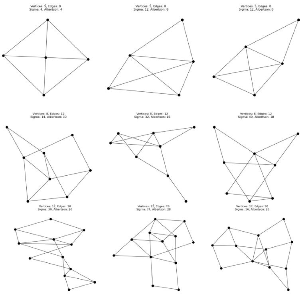
Figure 1. Compare value of the Sigma index and the Albertson index.

3. Upper Bound of Sigma Index

In this section, the upper bound of the Sigma index is characterized by encompassing several bounds. We observe through Proposition 3.1 a confinement of the Sigma index within the interval $[\frac{1}{3}\,,\frac{1}{10}]$ by considering the term $2n^{2}-1$. Lemma 3.1 presented the constant upper bound related to $n^{3}+m^{2}$.

Proposition 3.1.

Let $T$ be a tree, $\mathscr{D}(d_{1},d_{2},\dots,d_{n})$ be a degree sequence where $d_{1}\geqslant d_{2}\geqslant\dots\geqslant d_{n}$. Then, Sigma index satisfy

(1) $$~\frac{1}{3}<\left\lfloor\dfrac{2n^{2}-1}{2}\right\rfloor\dfrac{1}{\sigma(T)+d_{1}^{3}+(d_{1}-d_{2})^{3}-(d_{n-1}-d_{n})^{3}}<\frac{1}{10}.$$

Proof.

Assume $\mathscr{D}(d_{1},d_{2},\dots,d_{n})$ is a degree sequence where $d_{1}\geqslant d_{2}\geqslant\dots\geqslant d_{n}$ and the maximum degree $\Delta>3$. Since $n>\Delta$ and $2n^{3}+m>4\Delta$, the term $(2n^{3}+m/(4\Delta)$ yields the Sigma index that satisfies the relationship (2), where $\Delta\geqslant d_{1}$,

(2) $$~\sigma(T)\geqslant\left\lfloor\frac{2n^{3}+m}{4\Delta}\right\rfloor.$$

Let $k>0$ be an integer. Then, according to the required relationship (1), we observe that $k\leqslant n^{2}-\frac{1}{2}\leqslant k+1$. For $j\geqslant k$, according to (2), we find that $4\Delta j+4\Delta\leqslant 2n^{3}+m\leqslant 4\Delta j.$ Thus, according to relationship (2) we observe that

(3) $$~\left\lfloor\frac{2n^{3}+m}{4\Delta}\right\rfloor-\left\lfloor\frac{2n^{2}-1}{2}\right\rfloor\leqslant 4\Delta(k-j).$$

Therefore, the Sigma index satisfies $\sigma(T)>d_{1}^{3}+(d_{1}-d_{2})^{3}$. Next, for the term $d_{1}^{3}+(d_{1}-d_{2})^{3}$, we observe that

$$(d_{n-1}-d_{n})^{3}<d_{1}^{3}+(d_{1}-d_{2})^{3}<\sum_{i=1}^{n}d_{i}^{3},$$

which implies $\sigma(T)\geqslant d_{1}^{3}+(d_{1}-d_{2})^{3}-(d_{n-1}-d_{n})^{3}.$ Thus, according to (3), it holds that

(4) $$~\sigma(T)\geqslant\frac{d_{1}^{3}+(d_{1}-d_{2})^{3}-(d_{n-1}-d_{n})^{3}}{4\Delta(k-j)}.$$

Therefore,

(5) $$~1\leqslant\frac{d_{1}^{3}+(d_{1}-d_{2})^{3}-(d_{n-1}-d_{n})^{3}}{4\Delta(k-j)}\leqslant 3.$$

Thus, from (4) and (5), by adding the value of the Sigma index in relation (5), we conclude that (1) holds. ∎

Lemma 3.1.

Let $T$ be a tree and $\mathscr{D}(d_{1},d_{2},\dots,d_{n})$ be a degree sequence where $d_{1}\geqslant d_{2}\geqslant\dots\geqslant d_{n}$ with the maximum degree $\Delta$. Then,

(6) $$~0<\frac{1}{m-1}\left(\frac{2n^{3}+m^{2}}{\Delta(\Delta-1)^{2}}+\left\lfloor\frac{3nm}{7}\right\rfloor-\left\lceil\frac{3nm}{7}\right\rceil\right)<3,$$

if and only if $\sqrt{\sigma(T)}>n$.

Proof.

Consider $\mathscr{D}(d_{1},d_{2},\dots,d_{n})$ be a degree sequence where $d_{1}\geqslant d_{2}\geqslant\dots\geqslant d_{n}$ with the maximum degree $\Delta$ where $4\Delta\leqslant n$. Since $m=n-1$ and $2n^{3}+m^{2}=2n^{3}+n^{2}-2n+1$, we find that $2n^{3}+n^{2}-2n+1>\Delta(\Delta-1)^{2}$. For a certain term of $\Delta$, the lower bound of Sigma index satisfy:

(7) $$~\sigma(T)\geqslant\frac{2n^{3}+n^{2}-2n+1}{\Delta(\Delta-1)^{2}}+2n.$$

Thus, from (7) we noticed that $\sigma(T)>2n$ and $\sqrt{\sigma(T)}>n$. Therefore, we must prove under the assumption that the condition related to the Sigma index is satisfied according to equation (6). Here, let us discuss both the bounds and their relation to the Sigma index until we obtain the relation of these bounds through equation (6) with the Sigma index. Thus, we have:

(8) $$~\sigma(T)\leqslant\left\lfloor\frac{3nm}{7}\right\rfloor+\left\lceil\frac{3nm}{7}\right\rceil+2n^{2}+2,$$

where $2n^{2}+2$ is the constant term. Since $\sigma(T)>2n^{2}+2$ implies that $\sigma(T)>\left\lfloor\frac{3nm}{7}\right\rfloor+\left\lceil\frac{3nm}{7}\right\rceil.$ In this case, let $3<k<n/2$ and $k\in\mathbb{N}$. Then, according to (8) the lower bound of Sigma index satisfy

(9) $$~\sigma(T)\geqslant\left\lfloor\frac{knm}{k+4}\right\rfloor+\left\lceil\frac{knm}{k+4}\right\rceil.$$

Thus, according to both lower bounds (8) and (9) we find that

$$\sigma(T) \geqslant\left\lfloor\frac{knm}{k+4}\right\rfloor+\left\lceil\frac{knm}{k+4}\right\rceil$$

$$\geqslant\frac{1}{m-1}\left(\left\lfloor\frac{knm}{k+4}\right\rfloor+\left\lceil\frac{knm}{k+4}\right\rceil\right)$$

$$\geqslant\frac{1}{m-1}\left(\left\lfloor\frac{knm}{k+4}\right\rfloor+\left\lceil\frac{knm}{k+4}\right\rceil+2n^{2}+2\right).$$

Therefore, the lower bounds of Sigma index had discussed among (9) and (7). Thus, according to Proposition 3.1 we find that $\sigma(T)\geqslant\left\lfloor\frac{2n^{3}+m}{4\Delta}\right\rfloor$. Thus, it holds

(10) $$~n<\frac{1}{m-1}\left(\left\lfloor\frac{knm}{k+4}\right\rfloor+\left\lceil\frac{knm}{k+4}\right\rceil+2n^{2}+2\right)<n\Delta$$

Since $2n^{2}+2$ is the constant term and $\sigma(T)>2n^{2}+2$ according to (10) noticed that

(11) $$~2n<\frac{2n^{3}+n^{2}-2n+1}{\Delta(\Delta-1)^{2}}<n\Delta.$$

Thus, when $d_{1}\geqslant d_{2}\geqslant\dots\geqslant d_{n},$ we have $2n/(m-1)\approx 2$ and $n\Delta/(m-1)\leqslant n^{2}/\Delta$. Thus,

(12) $$~0<\frac{1}{m-1}\left(\frac{2n^{3}+n^{2}-2n+1}{\Delta(\Delta-1)^{2}}\right)<3.$$

Finally, according to (8) and (9) we find that the difference $\left\lfloor\frac{3nm}{7}\right\rfloor-\left\lceil\frac{3nm}{7}\right\rceil$ holds $\sigma(T)>\left\lceil\frac{3nm}{7}\right\rceil-\left\lfloor\frac{3nm}{7}\right\rfloor$. Then, by combining this results with (10), (11) and (12) we find that (6) holds. As desire. ∎

The sharp upper bound of Sigma index had disccused among Lemma 3.2, where we assume $d_{T}(v_{2})=d_{T}(v_{3})=\dots=d_{T}(v_{n-1})=k$. Sigma index satisfying $\sigma(T)=d_{1}(d_{1}-k)^{2}+d_{n}(k-d_{n})^{2}.$ Defining the sharp bounds, whether upper or lower, in the topological indices provides a clear indication of the extent to which these bounds approximate the actual values of the indicators, which is the objective we aim to achieve.

Lemma 3.2.

Let $T$ be a tree, let $\mathscr{D}(d_{1},d_{2},\dots,d_{n})$ be a degree sequence where $d_{1}\geqslant d_{2}\geqslant\dots\geqslant d_{n}$ with the maximum degree $\Delta$ and the minimum degree $\delta\geqslant 2$. Then, the upper bound of Sigma index satisfy

(13) $$~\sigma(T)\leqslant\left\lfloor\frac{3n}{5}\right\rfloor\left\lceil\frac{2n}{5}\right\rceil\frac{2nm}{\Delta(\Delta-1)^{2}}+\delta\sqrt{\frac{nm}{2\Delta(\Delta-1)}}+\frac{1}{2}(n^{2}+m^{2})+n(m-\Delta)^{2}.$$

Proof.

Assume $\mathscr{D}(d_{1},d_{2},\dots,d_{n})$ is a degree sequence where $d_{1}\geqslant d_{2}\geqslant\dots\geqslant d_{n}$ with maximum degree $\Delta$ and minimum degree $\delta\geqslant 2$. Let us have the following parameters $\alpha$, $\beta$, and $\gamma$, where

$$\alpha=\left\lfloor\frac{3n}{5}\right\rfloor\left\lceil\frac{2n}{5}\right\rceil,\quad\beta=\frac{1}{2}(n^{2}+m^{2}),\quad\gamma=n(m-\Delta).$$

Then, we notice that $\beta\geqslant\alpha+\gamma$. Thus, $\alpha$ satisfies the bound $\alpha\leqslant n\Delta+m$ and $\beta$ satisfies the bound $\beta\geqslant(m-1)^{2}+3n$. On the other hand, we observe that the bound according to $n,m,$ and $\Delta$ satisfies

$$3<\sqrt{\frac{nm}{2\Delta(\Delta-1)}}<4,\quad\text{where}\quad 0<\frac{2nm}{\Delta(\Delta-1)^{2}}<2.$$

Since $\mathscr{D}$ satisfies the order $d_{1}\geqslant d_{2}\geqslant\dots\geqslant d_{n}$, for any path in the tree, we observe that each of the vertices $V(T)=\{v_{1},v_{2},\dots,v_{n}\}$ satisfies $d_{T}(v_{1})>d_{T}(v_{2})\geqslant d_{T}(v_{3})\geqslant\dots\geqslant d_{T}(v_{n-1})>d_{T}(v_{n}).$ Hence, assume $d_{T}(v_{2})=d_{T}(v_{3})=\dots=d_{T}(v_{n-1})=k$. Then, the Sigma index satisfies

(14) $$~\sigma(T)=\sum_{v_{i}\in N(v_{1})}(d_{T}(v_{1})-k)^{2}+\sum_{v_{i}\in N(v_{n})}(k-d_{T}(v_{n}))^{2},$$

noting that all neighbors of $v_{1}$ and $v_{n}$ have degree $k$. Then, the Sigma index is $\sigma(T)=d_{T}(v_{1})(d_{T}(v_{1})-k)^{2}+d_{T}(v_{n})(k-d_{T}(v_{n}))^{2}.$ Actually, since $d_{1}\geqslant d_{2}\geqslant\dots\geqslant d_{n}$ in $\mathscr{D}$, we find that

$$\sigma(T)=d_{1}(d_{1}-k)^{2}+d_{n}(k-d_{n})^{2}.$$

Thus,

(15) $$~\sigma(T)\leqslant\alpha\sum_{v_{i}\in N(v_{1})}(d_{T}(v_{1})-k)^{2}+\gamma\sum_{v_{i}\in N(v_{n})}(k-d_{T}(v_{n}))^{2}.$$

Then, to determine the lower bound of the Sigma index according to parameters $\alpha$, $\beta$, and $\gamma$, and by considering equations (14) and (15), we find

(16) $$~\sigma(T)\geqslant\left\lfloor\frac{3n}{5}\right\rfloor\left\lceil\frac{2n}{5}\right\rceil\frac{2nm}{\Delta(\Delta-1)^{2}}+\sum_{v_{i}\in N(v_{1})}(d_{T}(v_{1})-\alpha)^{2}+\sum_{v_{i}\in N(v_{n})}(\gamma-d_{T}(v_{n}))^{2}.$$

Thus, these relations ultimately lead, according to the conditions we obtained in

$$3<\sqrt{\frac{nm}{2\Delta(\Delta-1)}}<4,\quad\text{ and }\quad 0<\frac{2nm}{\Delta(\Delta-1)^{2}}<2,$$

to the Sigma index satisfying relation (17), which represents the lower bound we want to achieve for the required relation (13) as:

(17) $$~\sigma(T)\leqslant\left\lfloor\frac{3n}{5}\right\rfloor\left\lceil\frac{2n}{5}\right\rceil\frac{2nm}{\Delta(\Delta-1)^{2}}+\frac{(n^{2}+m^{2})\sqrt{\frac{nm}{2\Delta(\Delta-1)}}}{2}.$$

Therefore, the term $n(m-\Delta)$ grows rapidly and according to (17), by combining it with $n(m-\Delta)$, the Sigma index satisfies the sharp upper bound. ∎

Throughout Theorem 3.3, we determine the relationship of the harmonic topological index and Sigma index according to Lemma 3.2.

Theorem 3.3.

Let $T$ be tree of order $n$, $H(G)$ be the harmonic topological index and let $\eta$ be an integer, $\mathscr{D}=(d_{1},d_{2},\dots,d_{n})$ be non-decreasing degree sequence with $\lambda_{\mathscr{D}}$ the average of elements $\mathscr{D}$. Then, the upper bound of Sigma index satisfy

(18) $$~\sigma(T)\leqslant\left\lfloor\frac{2n^{2}}{3\lambda_{\mathscr{D}}}\right\rfloor+\dfrac{2^{\eta}(m-\Delta)^{2}}{5(n-1)^{3}}+(n-1)H(G).$$

From the proof of Lemma 3.2, we would like to point out that the satisfied condition $3<\sqrt{nm/2\Delta(\Delta-1)}<4$ and $0<2nm/\Delta(\Delta-1)^{2}<2$ is also fulfilled for degree sequence $\mathscr{D}$ where $d_{1}\leqslant d_{2}\leqslant\dots\leqslant d_{n}$; hence, these bounds are considered to be confined by one or more increases.

Theorem 3.4 establishes the initial upper bounds by analyzing the sum of the squared differences between the degrees of $\mathscr{D}$, while considering the influence of the average relative to these degrees.

Theorem 3.4.

Let $T$ be a tree, and let $\mathscr{D}=(d_{1},d_{2},\dots,d_{n})$ be a degree sequence where $d_{1}\geqslant d_{2}\geqslant\dots\geqslant d_{n}$, with maximum degree $\Delta$, minimum degree $\delta\geqslant 2$, and let $\lambda_{\mathscr{D}}$ be the average of $\mathscr{D}$. Then, the upper bound of the Sigma index satisfies

(19) $$~\sigma(T)\leqslant\sum_{i=1}^{n-1}\lambda_{\mathscr{D}}(d_{i}-d_{i+1})^{3}+2(n^{2}+m^{2})+3m+n+2.$$

Proof.

Assume $\mathscr{D}(d_{1},d_{2},\dots,d_{n})$ is a degree sequence where $d_{1}\geqslant d_{2}\geqslant\dots\geqslant d_{n}$ with the maximum degree $\Delta$, the minimum degree $\delta\geqslant 2$, and $\lambda_{\mathscr{D}}$ the average of $\mathscr{D}$. It is clear that $n$ satisfies $n>\sum_{i=1}^{n-1}(d_{i}-d_{i+1})^{2}$ and $2n>\sum_{i=1}^{n-1}(d_{i}-d_{i+1})^{3}$. Both terms involving $n$ are essentially established for the lower bound with respect to the Sigma index. Thus, the lower bound of the Sigma index is

(20) $$~\sigma(T)\geqslant\sum_{i=1}^{n-1}\lambda_{\mathscr{D}}(d_{i}-d_{i+1})^{3}+2n^{2}+2.$$

According to Lemma 3.1, we compare the term $2n^{3}+n^{2}-2n+1$ with the term $\Delta(\Delta-1)^{2}$ by considering the value of $m-1,$

$$0<\frac{1}{m-1}\left(\frac{2n^{3}+n^{2}-2n+1}{\Delta(\Delta-1)^{2}}\right)<3.$$

Based on this reduction, the lower bound (20) is difficult to determine within a certain bound. Thus, we have

$$\Delta(n-\Delta)^{2}-\Delta(m-\Delta)^{2}\geqslant\sum_{i=1}^{n-1}\lambda_{\mathscr{D}}(d_{i}-d_{i+1})^{3},$$

and for the term $\Delta(\Delta-1)^{2}$ compared with the term $(2m^{2}+2m+n)/2(n+m)$, considering that $\sigma(T)<2m^{2}+2m+n$ holds, we obtain

$$(d_{1}-d_{n})^{2}\geqslant\frac{1}{\Delta(\Delta-1)^{2}}\left(\frac{2m^{4}+2m+n}{2(n+m)}\right).$$

The sharp lower bound of the Sigma index satisfies the inequality by considering (20) and the value of the term $(d_{1}-d_{n})^{2}$,

(21) $$~\sigma(T)>\frac{1}{\Delta(\Delta-1)^{2}}\left(\frac{2m^{4}+2m+n}{2(n+m)}+2nm+(d_{1}-d_{n})^{2}\right).$$

Thus, relationship (21) implies that $\Delta(2n-m)^{2}$ satisfies the lower bound according to the value of $\lambda_{\mathscr{D}}$ and the upper bound according to the value $d_{i}^{2}$. Hence,

(22) $$~\sum_{i=1}^{n-1}\lambda_{\mathscr{D}}(d_{i}-d_{i+1})^{3}\leqslant\frac{1}{4}\left(\frac{2m^{4}+2m+n}{2\Delta(n+m)(2n-m)^{2}}+2nm+(d_{1}-d_{n})^{2}\right)\leqslant 3\sum_{i=1}^{n}d_{i}^{2}-(n+m),$$

where

$$2\leqslant\frac{1}{4}\left(\frac{2m^{4}+2m+n}{2\Delta(n+m)(2n-m)^{2}}\right)\leqslant 3.$$

Therefore, from (21) and (22), the relationship with (20) implies (19). ∎

Actually, according to (20), (21) and (22) we obtain from discussing these bounds, we obtain the equivalent upper bound to the upper bound given in Theorem 3.4. This bound, which we obtain through Theorem 3.5, is a direct result of the discussion carried out through the relationships (20), (21) and (22).

Theorem 3.5.

For any tree $T$ with degree sequence $\mathscr{D}(d_{1},d_{2},\dots,d_{n})$ where $d_{1}\geqslant d_{2}\geqslant\dots\geqslant d_{n}$ and $\lambda_{\mathscr{D}}$ the average of $\mathscr{D}$. Then,according to Theorem 3.4 the upper bound of Sigma index satisfy

(23) $$~\sigma(T)\leqslant\sum_{i=1}^{n}d_{i}^{3}+\frac{2\lambda_{\mathscr{D}}(n^{2}+m^{2})}{3(n+m)}.$$

The following result is similarly achieved for the upper bound of the Sigma index, making it a sharply distinct and clear extreme value. Therefore, the approximate study to determine a specific sharp value for the Sigma index may not be consistent.

Corollary 3.6.

For any tree $T$ of order $n$. The upper bound of Sigma index satisfy

(24) $$~\sigma(T)\leqslant\sum_{i=1}^{n-1}\lambda_{\mathscr{D}}(d_{i}-d_{i+1})^{3}+2m^{2}+2m+n.$$

Corollary 3.7.

For any tree $T$ of order $n$. The upper bound of Sigma index satisfy

(25) $$~\sigma(T)\leqslant\sum_{i=1}^{n-1}\lambda_{\mathscr{D}}(d_{i}-d_{i+1})^{3}+2n^{2}+2.$$

Corollary 3.8.

For any tree $T$ of order $n$. Let $F(G)$ be the forgotten topological index. Then, the upper bound of Sigma index satisfy

(26) $$~\sigma(T)\leqslant 2F(G)+2n^{2}+2.$$

Proof.

According to the relationship of the forgotten topological index $F(G)$ and according to Theorem 2.1, we noticed that $\sigma(T)=F(G)+\sum_{uv\in E(G)}2d_{G}(u)d_{G}(v)$. Therefore,

$$\sum_{uv\in E(G)}(d_{G}(u)^{2}+d_{G}(v)^{2})>\sum_{uv\in E(G)}(d_{G}(u)-d_{G}(v))^{2}.$$

Thus, $\sigma(T)\leqslant 2F(G)$ and the term $2n^{2}+2$ is confirmed of the upper bound of Sigma index. ∎

Through the following table, we noticed that the degree sequences with corresponding values for Theorem 3.4, parameters $\alpha,\beta$ and $\gamma$, and values from Lemma 3.1.

Degree	Theorem 3.4	$\alpha$	$\beta$	$\gamma$	Lemma 3.1
(20,18,16,13,10,7,3)	30191	1820	7482.5	5742	2.158060942
(23,22,20,16,12,10,5)	46550	2816	34669.5	9072	2.144822168
(26,26,24,19,14,13,7)	66437	4004	49537.5	13158	2.08831593
(29,28,28,22,16,16,9)	87470	5280	65269.5	17464	1.959715692
(32,30,29,25,18,17,11)	104816	6305	78247.5	20898	1.733419168
(35,32,30,28,20,19,13)	125141	7526	93457.5	24957	1.570714215
(38,34,32,31,22,21,15)	148805	8970	111169.5	29729	1.450753316
(41,36,34,33,24,23,17)	172850	10416	129169.5	34528	1.335001258
(44,38,36,35,26,25,19)	198695	11970	148519.5	39694	1.23630804

Table 1. Present value of previous discussion with Lemma 3.1 and 3.2 and Theorem 3.4.

According to Table 1, we noticed that this analytical method aligns with standard techniques for sequence data (see Figure 2), aiming to identify patterns, correlations, and structural insights to comprehend the behavior of derived indices or parameters for specific degree sequences.

Figure 2. Explain the value among Table 1.

4. Lower Bounds of Sigma Index

In this section, The discussion previously presented in section 3 is continued, focusing on the analysis of the lower bound of the Sigma index. Both extreme values play a pivotal role in the behavior of the Sigma index, as illustrated in Figure 2. Through Proposition 4.1, we establish the lower bound of the Sigma index in accordance with Theorems 3.4 and 3.5, which were also employed to analyze the upper bound discussed earlier.

Proposition 4.1.

Let $T$ be a tree, $\mathscr{D}=(d_{1},d_{2},\dots,d_{n})$ be a degree sequence where $d_{1}\geqslant d_{2}\geqslant\dots\geqslant d_{n}$ and $M_{1}(T)$ be the first Zagreb index, and let $\lambda_{\mathscr{D}}$ be the average of $\mathscr{D}$. Then, the lower bound of the Sigma index satisfies

(27) $$~\sigma(T)\geqslant M_{1}(T)+\left\lfloor\frac{2(n+m)^{2}}{5}\right\rfloor+\frac{2\lambda_{\mathscr{D}}(n^{2}+m^{2})}{3(n+m)}.$$

Proof.

Assume $\mathscr{D}(d_{1},d_{2},\dots,d_{n})$ is a degree sequence where $d_{1}\geqslant d_{2}\geqslant\dots\geqslant d_{n}$ with the maximum degree $\Delta$ and $\lambda_{\mathscr{D}}$ is the average of $\mathscr{D}$. Since $2\lambda_{\mathscr{D}}(n^{2}+m^{2})>3(n+m)$ and $\Delta<\frac{2\lambda_{\mathscr{D}}(n^{2}+m^{2})}{3(n+m)}\leqslant 3\Delta$, according to Theorem 3.5 we find the upper bound of the Sigma index given as

$$\sigma(T)\leqslant\sum_{i=1}^{n}d_{i}^{3}+\frac{2\lambda_{\mathscr{D}}(n^{2}+m^{2})}{3(n+m)}.$$

Thus, let us consider the term $\Delta(\Delta-1)^{2}$ satisfies $\Delta(\Delta-1)^{2}<2(m+n)^{2}$. Then, we find that $\Delta(\Delta-1)^{3}\leqslant 2\lambda_{\mathscr{D}}(n^{2}+m^{2})$. Thus, the lower bound of the Sigma index satisfies

(28) $$~\sigma(T)\geqslant\Delta(\Delta-1)^{2}+\frac{2\lambda_{\mathscr{D}}(n^{2}+m^{2})}{3(n+m)}.$$

Therefore, from (28) we observe that this bound approaches the Sigma index very closely, due to the values of $\Delta$ that come from the condition we imposed on $\mathscr{D}$ where $d_{1}\geqslant d_{2}\geqslant\dots\geqslant d_{n}$. In this case, we note that the term $2(n+m)^{2}$ satisfies the relation $2(n+m)^{2}<\lambda_{\mathscr{D}}(n^{2}+m^{2})$. Therefore, we obtain the lower bound of the Sigma index as:

(29) $$~\sigma(T)\geqslant\left\lfloor\frac{2(n+m)^{2}}{5}\right\rfloor+\frac{2\lambda_{\mathscr{D}}(n^{2}+m^{2})}{3(n+m)}.$$

Hence, for the last term in (27) we notice that $\sum_{i=1}^{n}d_{i}^{2}<\Delta(\Delta-1)^{2}$. Thus, according to the lower bounds (28) and (29), the relationship (27) clearly holds. As desired. ∎

We observe from Proposition 4.1 that it directly leads to Corollary 4.1. Also, we notice through Equation (30) and by directly relying with the term $\sum_{i=1}^{n}d_{i}^{2}<\Delta(\Delta-1)^{2},$ that it gives us the lower bound of Sigma index.

Corollary 4.1.

For any tree $T$ of order $n$. The lower bound of Sigma index satisfy

(30) $$~\sigma(T)\geqslant\sum_{i=1}^{n-1}\lambda_{\mathscr{D}}(d_{i}-d_{i+1})^{2}+\left\lfloor\frac{2(n+m)^{2}}{5}\right\rfloor+\frac{2\lambda_{\mathscr{D}}(n^{2}+m^{2})}{3(n+m)}.$$

Based on Conjecture 1 which establishes Proposition 4.2, this conjecture is employed to refine the optimal terms that play a crucial role in enhancing the optimal behavior of the Sigma index.

Conjecture 1.

For any tree $T$ with $n$ vertices and $m$ edges. Let $k$ be an integer where $0<k<5$. Then,

(31) $$~0\leqslant\dfrac{2^{k}(n+m)^{2}}{2(k+1)\Delta(\Delta-1)^{2}}\leqslant 2k.$$

Proof.

Let $k$ be an integer where $0<k<5$, and assume $m=n-1$ in a tree $T$. Then the term $2^{k}$ with $(n+m)^{2}$ holds the bound $2^{k}<(n+m)^{2}$. Thus, clearly we find that:

(32) $$~\dfrac{2^{k}(n+m)^{2}}{2(k+1)}>0$$

Therefore, through relationship (32), the left-hand side of inequality (31) is satisfied when considering the term $\Delta(\Delta-1)^{2}$, which make (31) approach zero closely. Thus, for the right-hand side of the inequality (31), we find that $(n+m)^{2}/\Delta(\Delta-1)^{2}<2k$. Thus, for the term $2^{k}(n+m)^{2}$ is growing up. The right-hand side of inequality (31) is satisfied. ∎

Proposition 4.2.

Let $T$ be a tree and $\mathscr{D}(d_{1},d_{2},\dots,d_{n})$ be a degree sequence where $d_{1}\geqslant d_{2}\geqslant\dots\geqslant d_{n}$. Then, the lower bound of the Sigma index satisfies

(33) $$~\sigma(T)\geqslant d_{n}^{3}+d_{1}^{3}+\sum_{i=1}^{n-1}\frac{d_{i}}{d_{i+1}}+\left\lfloor\frac{n^{2}}{2}\right\rfloor+2n+2.$$

Proof.

Assume $\mathscr{D}(d_{1},d_{2},\dots,d_{n})$ is a degree sequence where $d_{1}\geqslant d_{2}\geqslant\dots\geqslant d_{n}$, and according to Conjecture 1, we noticed that $0<(n+m)^{2}/\Delta(\Delta-1)^{2}\leqslant 2$. Thus, we find that $d_{n}^{3}+d_{1}^{3}<\Delta(\Delta-1)^{2}$ and $\sigma(T)\leqslant d_{n}^{3}+d_{1}^{3}+\Delta(\Delta-1)^{2}$. Then,

(34) $$~\sigma(T)\geqslant d_{n}^{3}+d_{1}^{3}+\Delta(\Delta-1)^{2}-\left\lfloor\frac{n^{2}}{2}\right\rfloor.$$

Thus, for $d_{i}$ and $d_{i+1}$ we noticed that $1\leqslant d_{i}/d_{i+1}\leqslant 2$. Then,

$$\frac{(n+m)^{2}}{\Delta(\Delta-1)^{2}}\leqslant\sum_{i=1}^{n-1}\frac{d_{i}}{d_{i+1}}\leqslant 2n+2,$$

considering the fact that $0<(n+m)^{2}/\Delta(\Delta-1)^{2}\leqslant 2$. Thus, according to (34) we find that

(35) $$~\sigma(T)\geqslant d_{n}^{3}+d_{1}^{3}+\Delta(\Delta-1)^{2}+\sum_{i=1}^{n-1}\frac{d_{i}}{d_{i+1}}-\left\lfloor\frac{n^{2}}{2}\right\rfloor.$$

Therefore, the relationship (35) establishes the lower bound by comparing the terms as

$$\sigma(T) \geqslant d_{n}^{3}+d_{1}^{3}+\Delta(\Delta-1)^{2}+\sum_{i=1}^{n-1}\frac{d_{i}}{d_{i+1}}-\left\lfloor\frac{n^{2}}{2}\right\rfloor$$

$$\geqslant d_{n}^{3}+d_{1}^{3}+\Delta(\Delta-1)^{2}+\sum_{i=1}^{n-1}\frac{d_{i}}{d_{i+1}}-2n-2$$

$$\geqslant d_{n}^{3}+d_{1}^{3}+\sum_{i=1}^{n-1}\frac{d_{i}}{d_{i+1}}+\left\lfloor\frac{n^{2}}{2}\right\rfloor.$$

Thus, as we know, the value $2n+2$ is close to $2n$. Hence, we find that (33) holds. ∎

Furthermore, we observed that according to $\mathscr{D}$ where we optimize the terms $(d_{i}-d_{i+1})^{3}$ and $(d_{i}-d_{i+1})^{2}$. In fact, these terms significantly improve the determination of the lower bounds of the Sigma index, especially when studying the differences according to the given conditions in $\mathscr{D}$.

Lemma 4.2.

Let $T$ be a tree with $n$ vertices and $m$ edges. Let $\mathscr{D}(d_{1},d_{2},\dots,d_{n})$ be a degree sequence where $d_{1}\geqslant d_{2}\geqslant\dots\geqslant d_{n}$. The lower bound of Sigma index satisfies

(36) $$~\sigma(T)\geqslant\sum_{i=1}^{n-1}(d_{i}-d_{i+1})^{3}+\sum_{i=2}^{n-2}(d_{i}-d_{i+1})^{2}+d_{1}^{2}+d_{n}^{2}+\left\lfloor\frac{2(n+m)^{2}}{5}\right\rfloor.$$

Proof.

Assume $\mathscr{D}(d_{1},d_{2},\dots,d_{n})$ is a degree sequence where $d_{1}\geqslant d_{2}\geqslant\dots\geqslant d_{n}$. To determine the lower bound of the Sigma index given in equation (36), we will use mathematical induction. Consequently, we prove the validity of equation (36) for specific values of $n$, namely $n=4,5,6$.

For $n=4,$ we have

(37) $$~\sigma(T)\geqslant\sum_{i=1}^{n-1}(d_{i}-d_{i+1})^{3}+\sum_{i=2}^{n-2}(d_{i}-d_{i+1})^{2}+d_{1}^{2}+d_{n}^{2}+\left\lfloor\frac{2(n+m)^{2}}{5}\right\rfloor-n.$$

For $n=5$ we observe that

(38) $$~\sigma(T)\geqslant\sum_{i=1}^{n-1}(d_{i}-d_{i+1})^{3}+\sum_{i=2}^{n-2}(d_{i}-d_{i+1})^{2}+d_{1}^{2}+d_{n}^{2}+\left\lfloor\frac{2(n+m)^{2}}{5}\right\rfloor-2n.$$

Similarly, for $n=6$ we find

(39) $$~\sigma(T)\geqslant\sum_{i=1}^{n-1}(d_{i}-d_{i+1})^{3}+\sum_{i=2}^{n-2}(d_{i}-d_{i+1})^{2}+d_{1}^{2}+d_{n}^{2}+\left\lfloor\frac{2(n+m)^{2}}{5}\right\rfloor-3n.$$

From (37), (38), and (39), considering the term with respect to $n$ (since $m=n-1$), the relationship (36) holds true for $n=4,5,6$.

Assume the relationship is true for $n$; we must prove it for $n+1$. Therefore,

$$\sigma(T) \geqslant\sum_{i=1}^{n-1}(d_{i}-d_{i+1})^{3}+\sum_{i=2}^{n-2}(d_{i}-d_{i+1})^{2}+d_{1}^{2}+d_{n}^{2}+\left\lfloor\frac{2(n+m)^{2}}{5}\right\rfloor$$

$$\geqslant\sum_{i=2}^{n-2}(d_{i}-d_{i+1})^{3}+\sum_{i=1}^{n-3}(d_{i}-d_{i+1})^{2}+d_{1}^{2}+d_{n-1}^{2}+d_{n}^{2}+\left\lfloor\frac{2(n+m-2)^{2}}{5}\right\rfloor$$

$$\geqslant\sum_{i=2}^{n}(d_{i}-d_{i+1})^{3}+\sum_{i=3}^{n-1}(d_{i}-d_{i+1})^{2}+d_{1}^{2}+d_{n}^{2}+\left\lfloor\frac{2(n+m-2)^{2}}{5}\right\rfloor$$

$$\geqslant\sum_{i=3}^{n+1}(d_{i}-d_{i+1})^{3}+\sum_{i=4}^{n}(d_{i}-d_{i+1})^{2}+d_{1}^{2}+d_{n}^{2}+\left\lfloor\frac{2(n+m-3)^{2}}{5}\right\rfloor.$$

Note that the constant term is $\left\lfloor\frac{2(n+m)^{2}}{5}\right\rfloor$ and since $(d_{i}-d_{i+1})^{3}$ is positive due to the non-increasing order $d_{1}\geqslant d_{2}\geqslant\dots\geqslant d_{n}$, we have

(40) $$~\sigma(T)\geqslant n(d_{i}-d_{i+1})_{i\geqslant 1}^{3}+n(d_{i}-d_{i+1})_{i\geqslant 2}^{2}+d_{1}^{2}+d_{n}^{2}+\left\lfloor\frac{2(n+m-i)_{i\leqslant m}^{2}}{5}\right\rfloor.$$

Finally, from (39) and (40), we conclude that the lower bound of the Sigma index holds true for all $n+1$ and $n+2$. Thus, equation (36) is established. ∎

Similarly, according to Lemma 4.2 we obtained the following result such that we optimized the constant term $2(n+m-i)_{i\geqslant 2}^{2}$ with $n(d_{i}-d_{i+1})_{i\geqslant 1}^{3}$ and $n(d_{i}-d_{i+1})_{i\geqslant 2}^{2}$.

Corollary 4.3.

For any tree $T$ with $\mathscr{D}(d_{1},d_{2},\dots,d_{n})$ be a degree sequence where $d_{1}\geqslant d_{2}\geqslant\dots\geqslant d_{n}$. The lower bound of Sigma index satisfy

(41) $$~\sigma(T)\geqslant\sum_{i=1}^{n-1}(d_{i}-d_{i+1})^{4}+\sum_{i=2}^{n-2}(d_{i}-d_{i+1})^{3}+d_{1}^{2}+d_{n}^{2}+\left\lfloor\frac{2(n+m-2)^{2}}{5}\right\rfloor.$$

Throughout Corollary 4.3, discusses a clear case derived from Lemma 4.2. In this case, through both these results, we observed that among Theorem 4.4 which establishes an improvement in the lower bound for the Sigma index to be sufficiently close to Sigma index, and identifying it as a sharp and explicit value with respect to $\mathscr{D}$.

Theorem 4.4.

Let $T$ be a tree with $n$ vertices, $m$ edges, and the maximum degree $\Delta$. Let $\mathscr{D}(d_{1},d_{2},\dots,d_{n})$ be a degree sequence where $d_{1}\geqslant d_{2}\geqslant\dots\geqslant d_{n}$. The lower bound of the Sigma index satisfies

(42) $$~\sigma(T)\geqslant\sum_{i=1}^{n-1}(d_{i}-d_{i+1})^{4}+\sum_{i=2}^{n-2}(d_{i}-d_{i+1})^{3}+\sum_{i=1}^{n}d_{i}^{2}+d_{1}^{3}+d_{n}^{3}+2(d_{1}-d_{n})-n\Delta.$$

Proof.

Let $T$ be a tree with maximum degree $\Delta$ and $\mathscr{D}(d_{1},d_{2},\dots,d_{n})$ is a degree sequence where $d_{1}\geqslant d_{2}\geqslant\dots\geqslant d_{n}$. According to Lemma 4.2 we find that the lower bound of Sigma index satisfy

$$\sigma(T)\geqslant\sum_{i=1}^{n-1}(d_{i}-d_{i+1})^{3}+\sum_{i=2}^{n-2}(d_{i}-d_{i+1})^{2}+d_{1}^{2}+d_{n}^{2}+\left\lfloor\frac{2(n+m)^{2}}{5}\right\rfloor.$$

Then, we obtain from Corollary 4.3 another lower bound by considering the increase of the terms $(d_{i}-d_{i+1})^{3}$ and $(d_{i}-d_{i+1})^{2}$. Thus,

(43) $$~\sigma(T)\geqslant\sum_{i=1}^{n-1}(d_{i}-d_{i+1})^{4}+\sum_{i=2}^{n-2}(d_{i}-d_{i+1})^{3}.$$

For that reason, by returning to the discussion we presented in Lemma 4.2, we confirm that the relation (42) holds for $n=2,3,4$. Now, let us assume its validity for $n$ and prove that it also holds for $n+1$.

$$\sigma(T) \geqslant\sum_{i=1}^{n-1}(d_{i}-d_{i+1})^{4}+\sum_{i=2}^{n-2}(d_{i}-d_{i+1})^{3}+\sum_{i=1}^{n}d_{i}^{2}+d_{1}^{3}+d_{n}^{3}+2(d_{1}-d_{n})-n\Delta$$

$$\geqslant\sum_{i=1}^{n-2}(d_{i}-d_{i+1})^{4}+\sum_{i=1}^{n-3}(d_{i}-d_{i+1})^{3}+\sum_{i=1}^{n}d_{i}^{2}+d_{1}^{3}+d_{n-1}^{3}+2(d_{1}-d_{n-1})-2(n-1)\Delta$$

$$\geqslant\sum_{i=2}^{n}(d_{i}-d_{i+1})^{4}+\sum_{i=3}^{n-1}(d_{i}-d_{i+1})^{3}+\sum_{i=2}^{n+1}d_{i}^{2}+d_{1}^{3}+d_{n}^{3}-d_{n-1}^{3}+2(d_{1}-d_{n})+d_{n-1}-(n+1)\Delta$$

$$\geqslant\sum_{i=3}^{n+1}(d_{i}-d_{i+1})^{4}+\sum_{i=4}^{n}(d_{i}-d_{i+1})^{3}+\sum_{i=3}^{n+2}d_{i}^{2}+d_{1}^{3}+d_{n}^{3}-d_{n-2}^{3}-d_{n-1}^{3}+2(d_{1}-d_{n})-(n+2)\Delta.$$

Then, it holds the following relationship (44) by considering that the term $d_{i}-d_{i+1}$ satisfies $d_{i}-d_{i+1}\leqslant\Delta$, with the constant term $2(d_{1}-d_{n})$.

(44) $$~\sigma(T)\geqslant(n-1)\Delta^{4}-(n-3)\Delta^{3}+\sum_{i=3}^{n+2}(d_{1}+(i-1)\Delta)^{2}+\sum_{i=1}^{n}d_{i}^{3}-\left(\frac{3}{2}(d_{1}+d_{n})+(n+2)\Delta\right).$$

Thus, for the term $d_{1}^{3}+d_{n}^{3}$ we find that $d_{1}^{3}+d_{n}^{3}-d_{n-2}^{3}-d_{n-1}^{3}\leqslant\lfloor 2(n+m)^{2}/9\rfloor$. Then, for the constant term $2n-2$ where $2n-2>2(d_{1}-d_{n})$ we noticed that

(45) $$~\sigma(T)\geqslant\sum_{i=1}^{n-1}d_{i}(d_{i}-d_{i+1})^{4}+\sum_{i=2}^{n-2}d_{i}(d_{i}-d_{i+1})^{3}+2n-2.$$

Hence, from (45) for the term $d_{1}^{3}+d_{n}^{3}-d_{n-2}^{3}-d_{n-1}^{3}+2(d_{1}-d_{n})-(n+2)\Delta,$ we noticed that

(46) $$~\sigma(T)\geqslant\sum_{i=1}^{n-1}d_{i}(d_{i}-d_{i+1})^{4}+\sum_{i=2}^{n-2}d_{i}(d_{i}-d_{i+1})^{3}+(d_{1}-1)^{3}+(d_{n}-1)^{3}-(n+2)\Delta.$$

Finally, from (43)–(46) we find that the relationship (42) is true for $n+1$ and $n+2$. Thus, the lower bound of Sigma index (42) holds. ∎

The constant term has many cases to optimize the behavior of Sigma index such that in Theorem 4.5. Therefore, we consider the constant term had given as $\left\lfloor\frac{2n-1}{2}\right\rfloor\left\lceil\frac{3n-2}{3}\right\rceil$ by considering the value of $n$ and $\Delta$.

Theorem 4.5.

Let $T$ be a tree with $n$ vertices, $m$ edges, and the maximum degree $\Delta$. Let $\mathscr{D}(d_{1},d_{2},\dots,d_{n})$ be a degree sequence where $d_{1}\geqslant d_{2}\geqslant\dots\geqslant d_{n}$. The lower bound of the Sigma index satisfies

(47) $$~\sigma(T)\geqslant d_{1}^{3}+d_{n}^{3}+\sum_{i=2}^{n-1}(d_{i}-d_{i+1})^{4}+\left\lfloor\frac{2n-1}{2}\right\rfloor\left\lceil\frac{3n-2}{3}\right\rceil+\frac{1}{2}n\Delta.$$

Proof.

Assume $\mathscr{D}(d_{1},d_{2},\dots,d_{n})$ is a degree sequence where $d_{1}\geqslant d_{2}\geqslant\dots\geqslant d_{n}$. Then, according to Theorem 4.4, we find that

$$\sigma(T)\geqslant\sum_{i=1}^{n-1}(d_{i}-d_{i+1})^{4}+\sum_{i=2}^{n-2}(d_{i}-d_{i+1})^{3}.$$

Thus,

(48) $$~\sigma(T)\geqslant d_{1}^{3}+d_{n}^{3}+\sum_{i=2}^{n-1}(d_{i}-d_{i+1})^{4}.$$

Therefore, the lower bound discussed in Theorem 4.4 and Lemma 4.2 establishes the required lower bound in (47). Thus,

(49) $$~\sigma(T)\geqslant\sum_{i=1}^{n-1}(d_{i}-d_{i+1})^{3}+\sum_{i=2}^{n-2}(d_{i}-d_{i+1})^{2}+d_{1}^{3}+d_{n}^{3}.$$

Hence, from (48) and (49), we find that, for the value of $n$,

(50) $$~\sigma(T)\geqslant d_{1}^{3}+d_{n}^{3}+\left\lfloor\frac{2n-1}{2}\right\rfloor\left\lceil\frac{3n-2}{3}\right\rceil+\frac{1}{2}n\Delta.$$

Here, through relations (48), (49), and (50), relation (47) is satisfied for specific values of $n$. Therefore, suppose it holds for all values of $n$, and let us prove its validity for $n+1$. In this case, we find that relation (47) holds:

$$\sigma(T) \geqslant d_{1}^{3}+d_{n}^{3}+\sum_{i=2}^{n-1}(d_{i}-d_{i+1})^{4}+\left\lfloor\frac{2n-1}{2}\right\rfloor\left\lceil\frac{3n-2}{3}\right\rceil+\frac{1}{2}n\Delta$$

$$\geqslant d_{1}^{3}+d_{2}^{3}+d_{n-1}^{3}+\sum_{i=1}^{n-2}(d_{i}-d_{i+1})^{4}+\left\lfloor\frac{n-2}{2}\right\rfloor\left\lceil\frac{n-3}{3}\right\rceil+\frac{1}{2}n\Delta$$

$$\geqslant d_{1}^{3}+d_{n}^{3}+d_{n-1}^{3}+\sum_{i=3}^{n}(d_{i}-d_{i+1})^{4}+\left\lfloor\frac{n}{2}\right\rfloor\left\lceil\frac{n-2}{3}\right\rceil+\frac{1}{2}n\Delta-2(d_{1}+d_{n})^{2}$$

$$\geqslant d_{1}^{3}+d_{n}^{3}+d_{n-1}^{3}+d_{n-2}^{3}+\sum_{i=2}^{n-1}(d_{i}-d_{i+1})^{4}+\left\lfloor\frac{2n+1}{2}\right\rfloor\left\lceil\frac{3n+1}{3}\right\rceil+\frac{1}{2}n\Delta-2(d_{1}+d_{n}+d_{n-1})^{2}.$$

Therefore, by considering the term $\left\lfloor(2n-1)/2\right\rfloor\left\lceil(3n-2)/3\right\rceil$, we notice that the lower bound of the Sigma index satisfies

(51) $$~\sigma(T)\geqslant\sqrt{\sum_{i=1}^{n}d_{i}^{3}-\sum_{i=2}^{n-1}d_{i}^{2}}+\left\lfloor\frac{2n-1}{2}\right\rfloor\left\lceil\frac{3n-2}{3}\right\rceil+\frac{1}{2}n\Delta.$$

Finally, the term $\sqrt{\sum_{i=1}^{n}d_{i}^{3}-\sum_{i=2}^{n-1}d_{i}^{2}}$ grows the bound of the Sigma index and is closely related to the term $d_{1}^{3}+d_{n}^{3}$. Thus, we notice that (47) is valid for $n+1$ and $n+2$. Therefore, as the final result among all lower bounds (48)–(51), we find that (47) holds.

∎

5. Discussion The Effects of Bounds

From the results studied in Sections 3 and 4, we emphasize that the optimal behavior study of the Sigma index is conducted by evaluating the upper and lower bounds of the index along with some selected topological indices. According to Lemma 3.2, we find that we presented the upper bound of the Sigma index as

$$\sigma(T)\leqslant\left\lfloor\frac{3n}{5}\right\rfloor\left\lceil\frac{2n}{5}\right\rceil\frac{2nm}{\Delta(\Delta-1)^{2}}+\delta\sqrt{nm/2\Delta(\Delta-1)}+\frac{1}{2}(n^{2}+m^{2})+n(m-\Delta).$$

Also, we presented upper bound of the Sigma index through Theorem 3.4 as

$$\sigma(T)\leqslant\sum_{i=1}^{n-1}\lambda_{\mathscr{D}}(d_{i}-d_{i+1})^{3}+2(n^{2}+m^{2})+3m+n+2.$$

Hence, we observe that the difference making the upper bound sufficiently close is $n^{2}+m^{2}$ and $n(m-\Delta)$. Thus, we presented among Theorem 3.5, the relationship of the sharp upper bound of Sigma index with it collories as

$$\sigma(T)\leqslant\sum_{i=1}^{n}d_{i}^{3}+\frac{2\lambda_{\mathscr{D}}(n^{2}+m^{2})}{3(n+m)}.$$

Thus, let $k$ be an integer where $2\leqslant k<m-1$. Then, the upper bound of Sigma index associated with the terms $n^{2}+m^{2}$ and $n(m-\Delta)$. Therefore, the closest upper bound of Sigma index satisfy

(52) $$~\sigma(T)\leqslant k(n^{2}+m^{2})+n(km-\Delta).$$

From another perspective, based on PropositionS 4.1, 4.2 and Lemma 4.2, the fixed constant in each that ensures the lower bound closely approximates the Sigma index related to the term $\left\lfloor(2(n+m)^{2})/5\right\rfloor$. Consequently, by considering relation (52) and employing a similar reasoning, we derive the value that most accurately approaches the Sigma index through the tightest possible lower bound as:

(53) $$~\sigma(T)\geqslant\frac{1}{k}(n^{2}+m^{2})+\frac{1}{m-k}n(m-\Delta)+\left\lfloor\frac{2(n+m)^{2}}{5k}\right\rfloor.$$

Furthermore, from (52) and (53) we noticed that the difference between both bounds

$$k(n^{2}+m^{2})+n(km-\Delta)-\left(\frac{1}{k}(n^{2}+m^{2})+\frac{1}{m-k}n(m-\Delta)+\left\lfloor\frac{2(n+m)^{2}}{5k}\right\rfloor\right)$$

yield to

$$\frac{k^{2}-1}{k}(n^{2}+m^{2})+n\left(km-\Delta-\frac{m-\Delta}{m-k}\right)-\left\lfloor\frac{2(n+m)^{2}}{5k}\right\rfloor$$

Therefore, the difference provides the upper bound of Sigma index which we noticed that:

$$\sigma(T)<\frac{k^{2}-1}{k}(n^{2}+m^{2})+n\left(km-\Delta-\frac{m-\Delta}{m-k}\right)-\left\lfloor\frac{2(n+m)^{2}}{5k}\right\rfloor.$$

Enhancing the previous discussion, through Table 2 we demonstrate a comparison between the behavior of these extreme bounds, where we refer to the lower bound 1 (LB1) through Lemma 4.2 and to the lower bound 2 (LB2) through Theorem 4.4. Similarly, the upper bound 1 (UB1) refers to Lemma 3.2 and the upper bound 2 (UB2) refers to Theorem 3.4. The positions labeled $n,\sigma(T)$, LB1, LB2, UB1 and UB2 correspond to the variables whose pairwise correlation coefficients are displayed in the correlation matrix as

$$M_{\mathscr{D}}=\begin{pmatrix}1.000000&0.954243&0.985349&0.928820&0.956584&0.959995\\ 0.954243&1.000000&0.991001&0.996741&0.999966&0.999754\\ 0.985349&0.991001&1.000000&0.977349&0.992055&0.993259\\ 0.928820&0.996741&0.977349&1.000000&0.996057&0.995292\\ 0.956584&0.999966&0.992055&0.996057&1.000000&0.999862\\ 0.959995&0.999754&0.993259&0.995292&0.999862&1.000000\end{pmatrix}$$

Noticed that, regression coefficients $[\,-7.047368\,,-4.26834614\,]$, intercept $13518.783306538098$, Model $R^{2}$ is $0.9999999997765274$.

D	n	$\sigma(T)$	LB1	LB2	UB1	UB2
(15,13,11,10,8,6,4)	67	6318	7370	3293	179785.49	18349.43
(18,15,13,11,10,8,5)	80	10982	10553	5807	305555.00	26503.86
(21,17,15,12,12,10,7)	94	17714	14628	9543	498191.16	37144.43
(24,19,17,13,14,12,9)	108	26908	19403	14881	758415.44	50221.00
(27,21,19,14,16,14,11)	122	38972	24882	22235	1096368.79	66090.14
(30,23,21,15,18,16,13)	136	54314	31073	32091	1522259.18	85156.43
(33,25,23,16,20,18,15)	150	73342	37981	45007	2046200.62	107872.43
(36,27,25,17,22,20,17)	164	96464	45612	61613	2678413.08	134738.71
(39,29,27,18,24,22,19)	178	124088	53973	82611	3429033.56	166303.86
(42,31,29,19,26,24,21)	192	156622	63068	108775	4308189.06	203164.43

Table 2. Optimize of extremal bounds among Sigma index.

Through the following Figure 3, we present analyze the data among Table 2.

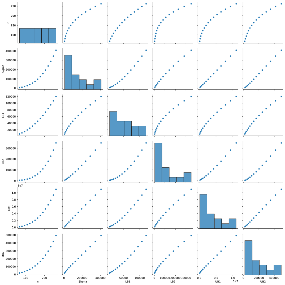
Figure 3. Analysis the extremal value by Table 2.

6. Conclusion

Through this paper, the study of the behavior of the effect of bounds on the Sigma index, considering the existence of many such bounds and their relation to harmonic topological indices as presented in Theorem 3.3, where we proved that the upper bound for the Sigma index is given by

$$\sigma(T)\leqslant\left\lfloor\frac{2n^{2}}{3\lambda_{\mathscr{D}}}\right\rfloor+\dfrac{2^{\eta}(m-\Delta)^{2}}{5(n-1)^{3}}+(n-1)H(G).$$

Similarly, for the forgotten topological index among Corollary 3.8, we showed that its relation with the Sigma index provides us with the upper bound for the Sigma index as follows $\sigma(T)\leqslant 2F(G)+2n^{2}+2.$ This study provides us with the behavior of extreme values that affect the Sigma index through both the upper and lower bounds.

The improvement of the upper bounds discussed through Lemma 3.1 and Lemma 3.2, and the enhancement of that discussion via Theorems 3.4 and 3.5, provide us with the strictest and most uniform bound. Through Section 4, we discussed the improvement of the lower bounds on the Sigma index, where we reinforced this discussion using Lemma 4.2 as well as Propositions 4.1 and 4.2, and we refined these results to appear in their complete forms through Theorems 4.4 and 4.5.

The study of the Sigma index through the optimal improvement regarding the effect of extremal bounds on the behavior of the index has a genuine and clear significance concerning the importance of these bounds and their impact on topological indices in general.

Declarations

• Funding: Not Funding.

• Conflict of interest/Competing interests: The author declare that there are no conflicts of interest or competing interests related to this study.

• Ethics approval and consent to participate: The author contributed equally to this work.

• Data availability statement: All data is included within the manuscript.

References

- [1] H. Abdo, S. Brandt, D. Dimitrov, The total irregularity of a graph, Discrete Mathematics & Theoretical Computer Science. 16(1) (2014), 201–206.
- [2] H. Abdo, D. Dimitrov, Non-regular graphs with minimal total irregularity, B. Aust. Math. Soc. 92 (2015) 1–10.
- [3] H. Abdo, D. Dimitrov, & I. Gutman, Graphs with maximal -irregularity, Discrete Appl. Math. 250 (2018) 57–64.
- [4] H. Abdo, D. Dimitrov, I. Gutman, Graph irregularity and its measures, Applied Mathematics and Computation. 357 (2019), 317–324.
- [5] A. Ali, A. M. Albalahi, A. M. Alanazi, A. A. Bhatti, & A. E. Hamza, On the maximum sigma index of k-cyclic graphs, Discrete Applied Mathematics. 325 (2023), Pages 58-62, https://doi.org/10.1016/j.dam.2022.10.009.
- [6] A. Alia, D. Dimitrovb, T. Rétic, A. M. Albalahia, & A. E. Hamzaa, Bounds and Optimal Results for the Total Irregularity Measure, MATCH Commun. Math. Comput. Chem. 94 (2025) 5–29, doi:10.46793/match.94-1.005A.
- [7] L. Alex, G. Indulal, & J. J. Mulloor, On the inverse problem of some bond additive indices, Communications in Combinatorics and Optimization. 2024.
- [8] N. Akgüneş, Y. Nacaroğlu, On the sigma index of the corona products of monogenic semigroup graphs, Journal of Universal Mathematics. 2(1) (2019), 68-74.
- [9] M. Ascioglu, I. N. Cangul, Sigma index and forgotten index of the subdivision and r-subdivision graphs, In Proceedings of the Jangjeon Mathematical Society. 21(2) (2018), pp. 1-14.
- [10] M. O. Albertson, The irregularity of a graph, Ars Combinatoria. 46 (1997), 219–225.
- [11] A. Arif, S. Hayat, & A. Khan, On irregularity indices and main eigenvalues of graphs and their applicability, Journal of Applied Mathematics and Computing, 69(3) (2023), 2549-2571.
- [12] I. I. Baskin, E. V. Gordeeva, R. O. Devdariani, N. S. Zefirov, V. A. Palyulin, M. I. Stankevich, Methodology for solving the inverse problem of structure-property relationships for the case of topological indexes, Dokl. Akad. Nauk SSSR 307 (1989) 613–617.
- [13] Y. Caro, R. Pepper, Degree sequence index strategy, Australasian Journal of Combinatorics. 59(1) (2014), 1-23.
- [14] G. Chartrand, F. Okamoto, & P. Zhang, The sigma chromatic number of a graph, Graphs and combinatorics. 26(6) (2010), 755-773, doi:10.1007/s00373-010-0952-7.
- [15] Z. Che, Z. Chen, Lower and upper bounds of the forgotten topological index, MATCH Commun. Math. Comput. Chem, 76(3) (2016), 635-648.
- [16] X. Chen, X. Liu, The reciprocal irregularity of a graph. Discrete Applied Mathematics, 378, 348-357.
- [17] Z. Du, A. Jahanbai, & S. M. Sheikholeslami, Relationships between Randic index and other topological indices, Communications in Combinatorics and Optimization. 6(1) (2021), 137-154.
- [18] D. Dimitrov, D. Stevanović, On the -irregularity and the inverse irregularity problem, Appl. Math. Comput. 441 (2023) 127709.
- [19] S. Fajtlowicz, On conjecture sofGrati–II, Congr.Numer.,60(1987),187–197.
- [20] S. Filipovski, D. Dimitrov, M. Knor, & R. Škrekovski, Some results on -irregularity arXiv e-prints, arXiv-2411.
- [21] B. Furtula, I. Gutman, A forgotten topological index, J. Math. Chem. 53 (2015) 11841190.
- [22] W. Gao, W. Wang, M. R. Farahani, Topological Indices Study of Molecular Structure in Anticancer Drugs, Hindawi Publishing Corporation Journal of Chemistry, (2016), http://dx.doi.org/10.1155/2016/3216327.
- [23] D. u. Gómez, Y. Grandati, & R. Milson,Rational extensions of the quantum harmonic oscillator and exceptional Hermite polynomials, Journal of Physics A: Mathematical and Theoretical. 47(1) (2013), 015203, doi:10.1088/1751-8113/47/1/015203.
- [24] I. Gutman, Topological indices and irregularity measures, Bulletin of International Mathematical Virtual Institute. 8 (2018), 469-475.
- [25] I. Gutman, M. Togan, A. Yurttas, A. S. Cevik, I. N. Cangul, Inverse problem for sigma index, MATCH Commun. Math. Comput. Chem. 79(3) (2018), 491–508.
- [26] I. Gutman, B. Ruščić, N. Trinajstić, C. F. Wilcox, Graph theory and molecular orbitals. XII. Acyclic polyenes, The Journal of Chemical Physics. 62(9) (1975), 3399–3405.
- [27] I. Gutman, N. Trinajstić, Graph theory and molecular orbitals. Total -electron energy of alternant hydrocarbons, Chemical Physics Letters. 17(4) (1972), 535–538.
- [28] J. Hamoud, D. Abdullah, Topological Indices with Degree Sequence of Tree, Lobachevskii Journal of Mathematics. 46(8) (2025), pp. 4249–4264, doi: 10.1134/S1995080225606769.
- [29] J. Hamoud, D. Abdullah, Albertson index and Sigma index in trees given by degree sequences, Chebyshevskii sbornik. 26(3) (2025), doi: 10.22405/2226-8383-2025-26-3-2-11.
- [30] S. L. Hakimi, On the realizability of a set of integers as degrees of the vertices of a graph, SIAM Journal on Applied Mathematics. 10 (1962), 496–506.
- [31] M. Knor, R. S̃krekovski, S. Filipovski, D. Dimitrov, Extremizing antiregular graphs by modifying total -irregularity, Applied Mathematics and Computation, 490 (2025), 129199, https://doi.org/10.1016/j.amc.2024.129199.
- [32] Z. Lingping, The harmonic index for graphs, Applied Mathematics Letters. 25(3) (2012), PP 561-566, https://doi.org/10.1016/j.aml.2011.09.059.
- [33] M. Matejić, I. Milovanović, & E. Milovanović, On bounds for harmonic topological index, Filomat, 32(1) (2018), 311-317.
- [34] M. R. Oboudi, A new lower bound for the energy of graphs, Linear Algebra Appl. 580 (2019), 384395.
- [35] P. B. Sarasija, R. Binthiya, Bounds on the Seidel energy of strongly quotient graphs, J. Chem. Pharm. Sci. 10 (1) (2017),p 14.
- [36] D. C. Schmidt, L. E. Druffel, A fast backtracking algorithm to test directed graphs for isomorphism using distance matrices, Journal of the ACM (JACM), 23(3) (1976), 433-445.
- [37] J. M. Sigarreta, Mathematical properties of variable topological indices, Symmetry, 13(1) (2020), 43.
- [38] D. Vukicevic, B. Furtula, Topological index based on the ratios of geometrical and arithmetical means of end-vertex degrees of edges, J. Math. Chem. 46(4) (2009), 13691376.
- [39] A. Vasilyev, R. Darda, & D. Stevanović, Trees of given order and independence number with minimal first Zagreb index, MATCH Commun. Math. Comput. Chem. 72 (2014), 775-782.
- [40] Z. Yang, M. Arockiaraj, S. Prabhu, M. Arulperumjothi, & J. B. Liu, Second Zagreb and sigma indices of semi and total transformations of graphs, Hindawi Complexity. 1 (2021), 6828424, https://doi.org/10.1155/2021/6828424.
- [41] A. Jahanbanı, S. Ediz, The sigma index of graph operations, Sigma Journal of Engineering and Natural Sciences. 37(1) (2019), 155-162.