The age and metallicity dependence of the near-infrared absolute magnitude and colour of red clump stars

Abstract

Understanding the age and metallicity dependence of the absolute magnitude and colour of red clump (RC) stars is crucial for validating the accuracy of stellar evolution models and enhancing their reliability as a standard candle. However, this dependence has previously been investigated in the near-infrared across multiple bands only for -1.05 $\leq$ [Fe/H] $\leq$ 0.40, a range accessible through the star clusters in the Large Magellanic Cloud. Therefore, we used star clusters in the Small Magellanic Cloud and the Milky Way Galaxy to investigate the age and metallicity dependence of the absolute magnitude and colour of RC stars in the near-infrared for a broader parameter space (0.45 $\leq$ Age (Gyr) $\leq$ 10.5, -1.65 $\leq$ [Fe/H] $\leq$ 0.32). Comparison of our results with three isochronous models BaSTI, PARSEC, and MIST reveals that the age dependence of the absolute magnitude for young RC stars aligns well with theoretical predictions, within the fitting errors of the multiple regression analysis. Additionally, the observed colour shows good agreement with the theoretical models. Notably, the $J-K_{S}$ colour, which spans a wide parameter space, reproduces the distribution expected from the theoretical model.

1 Introduction

Red clump (RC) stars are core helium-burning stars that have evolved from relatively metal-rich low-mass stars. These stars are widely used as a standard candle for determining the structure of the Milky Way Galaxy and measuring the distance to nearby galaxies. Additionally, RC stars serve as a "standard crayon" for investigating interstellar extinction due to their small variations in luminosity and colour, as well as their significant population density.

However, it is now established that the absolute magnitude and colour of RC stars exhibit an age and metallicity dependence (population effect), albeit not a strong one. Theoretically, the population effect of RC stars has been investigated by Girardi & Salaris (2001) and Salaris & Girardi (2002). A precise understanding of this population effect is crucial for validating the accuracy of stellar evolution models and for employing it as a more reliable standard candle with population effect corrections. Observational verification of the population effect remains limited because of the difficulty in determining the age of RC stars.

One approach to estimating the age of RC stars is to use star clusters. The age of a star cluster can be estimated by comparing its colour-magnitude diagram with isochrones derived from theoretical models. Several studies have used star clusters in the Milky Way Galaxy to investigate the population effects on the absolute magnitude of RC stars (Grocholski & Sarajedini, 2002; Percival & Salaris, 2003; van Helshoecht & Groenewegen, 2007). Onozato et al. (2019) used star clusters in the Large Magellanic Cloud (LMC) to study the population effects of absolute magnitude and colour of RC stars. Another method for estimating the age of RC stars is using asteroseismology, although this approach is associated with significant age uncertainties (Chen et al., 2017).

In this study, we analyse the colour of RC stars using star clusters from the Small Magellanic Cloud (SMC) and the Magellanic Bridge (MB), as well as the absolute magnitude and colour of RC stars using star clusters in the Milky Way Galaxy in addition to the LMC results of Onozato et al. (2019). The target clusters differ from those in the LMC in terms of age and metallicity: the clusters in the SMC and MB are older and have lower metallicity, while the open clusters in the Milky Way Galaxy have higher metallicity, thereby expanding the parameter space for investigating population effects. Additionally, the star clusters in each galaxy or region have an age-metallicity relation, where younger clusters have higher metallicity and older clusters have lower metallicity, making it difficult to study the effects of age and metallicity independently. However, because the SMC and MB have extended structures along the line of sight and cannot be considered equidistant, unlike the star clusters in the LMC, only the colour of the star clusters in the SMC is analysed.

Section 2 describes the data and Section 3 presents methods employed to select the star clusters and to determine the absolute magnitude and colour of the RC stars. Section 4 discusses the results obtained from these methods, while Section 5 provides the conclusions.

2 The Data

2.1 SMC star clusters data

We used the catalogue of Bica et al. (2020) as a list of star clusters in the SMC and the MB. This catalogue includes star clusters, associations, and related extended objects in the SMC and the MB. We chose objects classified as type C, denoting resolved star clusters, as the sample for this study. Among these, 117 star clusters have both age and metallicity measurements.

The near-infrared (NIR) magnitude of the individual members of the star clusters was obtained from the VISTA survey of the Magellanic Clouds (VMC survey) data release (DR) 5.1 (Cioni et al., 2011). The VMC survey is a NIR survey in the $Y$, $J$, and $K_{s}$ bands of the Magellanic Cloud system conducted with the Visible and Infrared Survey Telescope for Astronomy (VISTA telescope; Emerson et al., 2006) and equipped with the VISTA infrared camera (VIRCAM; Dalton et al., 2006). Data for the SMC, the MB and the Magellanic Stream are available in the VMC DR5.1. Given the crowded nature of these regions, we used the catalogue of point spread function (PSF) fitting photometry. Of the 117 star clusters listed in the catalogue of Bica et al. (2020), 109 are included in the VMC survey area.

2.2 Milky Way star clusters data

The star clusters catalogue of van Helshoecht & Groenewegen (2007) was employed to select the target star clusters in the Milky Way Galaxy. Near-infrared photometric data were acquired from the Two Micron All Sky Survey (2MASS, Skrutskie et al., 2006). The 2MASS is a near-infrared $J$, $H$, and $K_{S}$-band survey conducted using 1.3-m telescopes at Mount Hopkins, Arizona and Cerro Tololo, Chile. The 10 $\sigma$ detection limits are 15.8, 15.1, 14.3 mag at the $J$, $H$, $K_{S}$ bands, respectively, which are adequate for Milky Way star clusters. Age, metallicity, and $E(B-V)$ of the star clusters were taken from Kharchenko et al. (2013). The true distance moduli (DM) of the star clusters were determined from the mean parallax of the member stars ($\omega$, the unit is arcsec), as provided by in Cantat-Gaudin & Anders (2020) using the formula:

$$DM=5\log\omega-5.$$ (1)

3 Method

3.1 Determination of the absolute magnitude and colour of the RC stars in each cluster

3.1.1 SMC star clusters

The colour of the RC stars was determined using a method similar to Onozato et al. (2019). First, stars in star clusters were selected based on the mean values of the semi-major and semi-minor axes described in Bica et al. (2020). Figs. 1 and 2 show the colour-magnitude diagrams (CMDs) for the selected stars of target star clusters in the SMC. We chose stars with $18.5<m_{K_{S}}<15.5$ and $0.2<J-K_{S}<0.8$ to determine the average colour of the RC stars in the star clusters. Next, we obtained the $m_{K_{S}}$ histograms for the rectangle region in CMDs containing RC stars as shown in Fig. 3. The control fields were defined as circular rings with inner radii equal to those of the star clusters and outer radii extending to the radii of the star cluster + 1.5 arcmin. The $m_{K_{S}}$ histograms of the field stars were normalised to the ones that correspond to the same area as the target star clusters. Subsequently, these field $m_{K_{S}}$ histograms were subtracted from the cluster histograms, isolating the genuine cluster $m_{K_{S}}$ diagrams for analysis. The number of stars was normalised by the area of the star cluster when the histograms were created. For Lindsay 1, the outer radius of the surrounding region was set to the star cluster radius + 1.2 arcmin because of the discontinuity in the stellar density distribution at the border of the observed region. The apparent magnitude of selected stars were fitted with the following functional form as Girardi (2016)

$$N(m_{\lambda})=a+bm_{\lambda}+cm_{\lambda}^{2}+d\exp\left[-\frac{(m_{\lambda}^{RC}-m_{\lambda})^{2}}{2\sigma_{\lambda}^{2}}\right],$$ (2)

where $\lambda$ is a passband ($YJK_{S}$). The quadratic term represents the distribution of red giant branch stars, while the Gaussian term corresponds to the distribution of RC stars. $m_{\lambda}^{\mathrm{RC}}$ is the mean apparent magnitude and $\sigma_{\lambda}$ is the standard deviation of the RC stars. The number of RC stars ($N_{\mathrm{RC}}$) to calculate standard errors are given by

$$N_{\mathrm{RC}}=\sqrt{2\pi}\sigma_{\lambda}\times 10d.$$ (3)

A total of 28 star clusters could be fitted using this formula. The number of star clusters in each selection process is shown in Table 1. We corrected interstellar extinction using $E(B-V)$ values of Bica et al. (2020), as shown in Table 2, and the extinction law of Cardelli et al. (1989). We adopted the $R_{V}$ value of 3.1. The colour of the RC stars for each cluster was derived by subtracting the magnitude in each passband determined through this procedure.

Information on the star clusters for which the colour of RC stars has been derived is summarised in Table 2. Fig. 4 shows the age and metallicity distribution of the star clusters for which the absolute magnitude or colour of the RC stars has been determined in this work and previous studies. It can be seen that our sample includes many metal-poor and old star clusters that have not been previously covered.

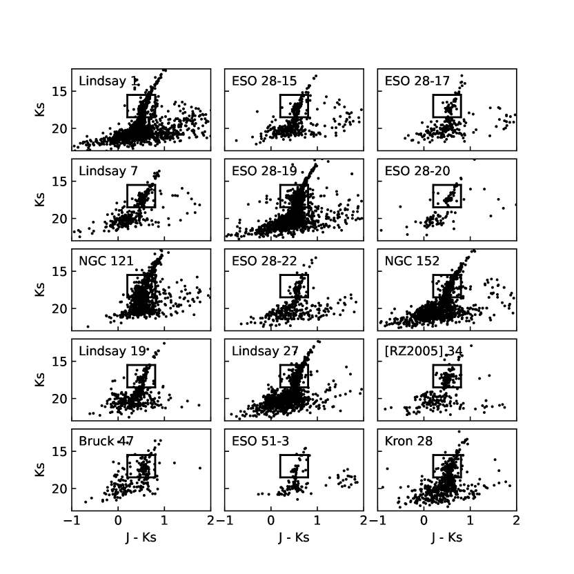
Figure 1: $J-K_{S}$ versus $K_{S}$ colour magnitude diagrams of our target star clusters of the SMC. The black rectangles represent the boundary to select the stars for fitting.

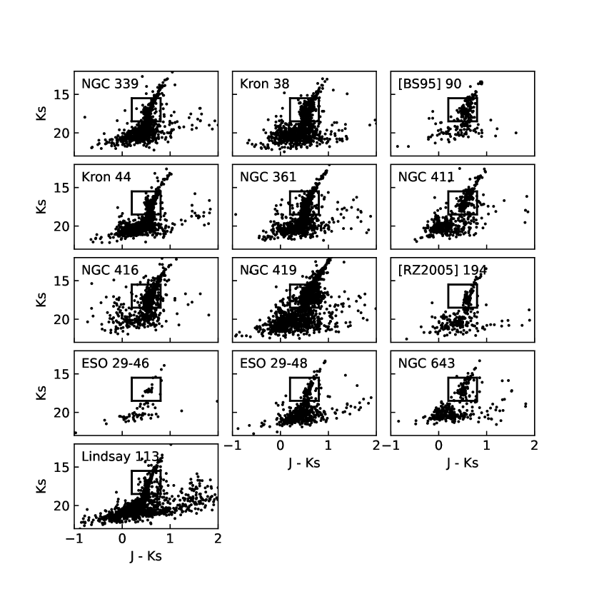
Figure 2: Continued from Fig. 1.

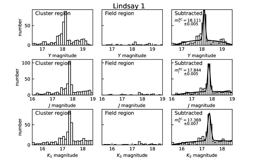
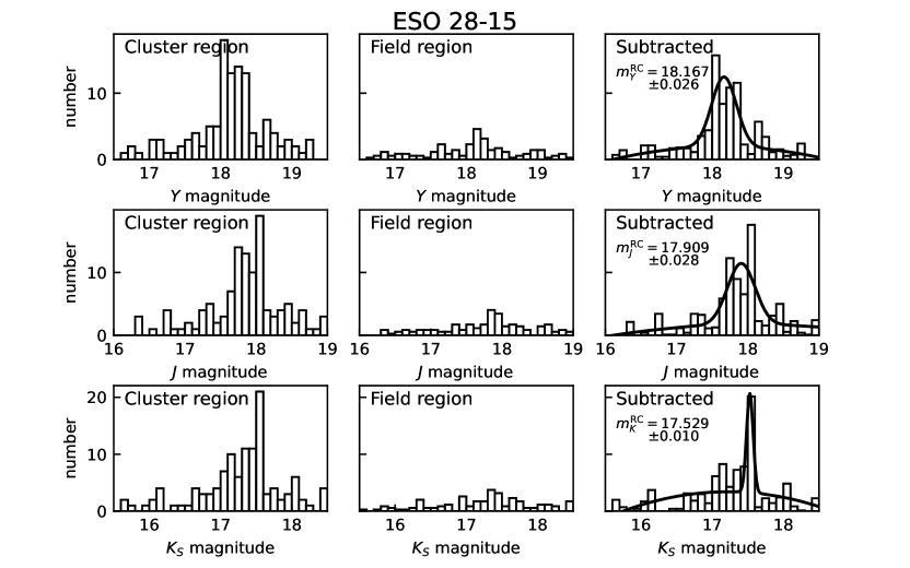
Figure 3: The luminosity functions of the RC stars as a function of their magnitude in the $Y$- (top), $J-$ (centre), and $K_{S}$-bands (bottom) for Lindsay 1 and ESO 28-15. (left) The luminosity functions of the cluster region. (centre) The luminosity functions of the field region. (right) The luminosity functions of the star cluster. The luminosity functions of the field region are subtracted from that of the cluster region. The fitting results with the equation (2) are shown by red lines.

Table 1: The number of star clusters at each selection process

Selection process	number of clusters
All objects in Bica et al. (2020)	2741
All star clusters (Type of object is C) in Bica et al. (2020)	626
Star clusters with age and metallicity	117
Star clusters in the VMC survey region	109
Star clusters that have significant RC excess and can be fitted by equation (2)	28

Table 2: SMC Cluster Information

Cluster name	RA (J2000.0)	Dec (J2000.0)	Radius (arcmin)	Age (Gyr)	[Fe/H]	$E(B-V)$	Age Ref.a	[Fe/H] Ref.a	$E(B-V)$ Ref.a
Lindsay 1	00h 03m 54$\aas@@fstack{s}$6	-73°28′16″	2.3	$7.5\pm 0.5$	$-1.04\pm 0.04$	0.019b	(1)	(2)	(1)
ESO 28-15	00h 21m 27$\aas@@fstack{s}$3	-73°44′53″	1.1	$5.1^{+2.8}_{-1.8}$ c	$-1.08\pm 0.04$	0.04	(3)(4)d	(5)	(6)
ESO 28-17	00h 23m 04$\aas@@fstack{s}$0	-73°40′12″	0.85	$5.3^{+3.4}_{-2.0}$ c	$-1.24\pm 0.03$	0.03	(3)(6)	(5)	(6)
Lindsay 7	00h 24m 43$\aas@@fstack{s}$16	-73°45′11$\aas@@fstack{\prime\prime}$7	0.9	1.4e	$-0.76\pm 0.06$	0.02	(3)(6)	(5)	(6)
ESO 28-19	00h 24m 46$\aas@@fstack{s}$0	-72°47′38″	1.7	$6.5\pm 0.5$	$-0.85\pm 0.03$	0.019b	(1)	(2)	(1)
ESO 28-20	00h 25m 26$\aas@@fstack{s}$60	-74°04′29$\aas@@fstack{\prime\prime}$7	0.50	$1.6\pm 0.4$	$-0.63\pm 0.02$	0.03	(7)	(2)	(7)
NGC 121	00h 26m 48$\aas@@fstack{s}$5	-71°32′05″	1.725	$10.5\pm 0.5$	$-1.19\pm 0.12$	0.027b	(8)	(9)	(8)
ESO 28-22	00h 27m 45$\aas@@fstack{s}$17	-72°46′52$\aas@@fstack{\prime\prime}$5	0.85	$3.5\pm 1.0$	$-0.81\pm 0.13$	0.040	(10)	(9)	(10)
NGC 152	00h 32m 56$\aas@@fstack{s}$3	-73°06′57″	1.5	$1.23\pm 0.07$	$-0.80\pm 0.30$	$0.03\pm 0.01$	(4)	(9)	(4)
Lindsay 19	00h 37m 41$\aas@@fstack{s}$78	-73°54′19$\aas@@fstack{\prime\prime}$7	0.85	4.0e	$-0.87\pm 0.03$	0.02	(3)(6)	(5)	(6)
Lindsay 27	00h 41m 24$\aas@@fstack{s}$2	-72°53′27″	1.25	$4.6\pm 0.6$	$-1.14\pm 0.06$	0.11	(3)	(5)	(6)
[RZ2005] 34	00h 42m 59$\aas@@fstack{s}$87	-72°35′21$\aas@@fstack{\prime\prime}$0	0.50	$0.70\pm 0.10$	$-0.40\pm 0.22$	$0.000\pm 0.010$	(3)	(11)	(11)
Bruck 47	00h 48m 33$\aas@@fstack{s}$23	-73°18′25$\aas@@fstack{\prime\prime}$1	0.50	$1.29_{-1.9}^{+1.1}$ c	$-0.01\pm 0.12$	$0.080\pm 0.030$	(3)(12)	(11)	(11)
ESO 51-3	00h 48m 50$\aas@@fstack{s}$0	-69°52′12″	0.90	$6.0_{-0.4}^{+0.5}$ c	$-1.65\pm 0.20$	0.013b	(1)(3)(13)	(13)	(1)
Kron 28	00h 51m 39$\aas@@fstack{s}$55	-71°59′56$\aas@@fstack{\prime\prime}$6	0.85	$2.0\pm 0.3$	$-1.20\pm 0.20$	0.06	(3)	(13)	(13)
NGC 339	00h 57m 47$\aas@@fstack{s}$5	-74°28′17″	1.45	$6.0\pm 0.5$	$-1.19\pm 0.10$	0.032	(1)	(9)	(1)
Kron 38	00h 57m 49$\aas@@fstack{s}$5	-73°25′23″	1.1	$3.0\pm 0.4$	$-0.88\pm 0.65$	$0.010\pm 0.020$	(3)	(11)	(11)
[BS95] 90	00h 59m 07$\aas@@fstack{s}$25	-72°08′59$\aas@@fstack{\prime\prime}$1	0.50	$4.5\pm 0.5$	$-0.80^{f}$	0.021	(14)	(15)	(14)
Kron 44	01h 02m 04$\aas@@fstack{s}$0	-73°55′33″	1.45	$3.0\pm 0.3$	$-0.81\pm 0.04$	0.05	(3)	(2)	(13)
NGC 361	01h 02m 11$\aas@@fstack{s}$0	-71°36′21″	1.3	$8.10\pm 1.20$	$-1.45\pm 0.11$	$0.07\pm 0.03$	(16)	(16)	(16)
NGC 411	01h 07m 55$\aas@@fstack{s}$3	-71°46′04″	1.05	$1.5\pm 0.3$ g	$-0.84\pm 0.30$	0.03	(7)(17)(18)(19)	(9)	(7)
NGC 416	01h 07m 59$\aas@@fstack{s}$0	-72°21′20″	0.85	$6.0\pm 0.5$	$-1.44\pm 0.12$	$0.08\pm 0.03$	(1)	(16)	(16)
NGC 419	01h 08m 18$\aas@@fstack{s}$0	-72°53′02″	1.4	$1.4\pm 0.2$	$-0.70\pm 0.30$	0.083b	(1)	(9)	(1)
[RZ2005] 194	01h 12m 51$\aas@@fstack{s}$74	-73°07′10$\aas@@fstack{\prime\prime}$9	0.60	$4.1\pm 0.3$	$-0.88\pm 0.65$	$0.040\pm 0.010$	(3)	(11)	(20)
ESO 29-46	01h 33m 14$\aas@@fstack{s}$0	-74°10′00″	0.60	$3.6^{+0.4}_{-0.3}$ c	$-0.88\pm 0.65$	$0.010\pm 0.005$	(3)(21)	(11)	(11)
ESO 29-48	01h 34m 26$\aas@@fstack{s}$0	-72°52′28″	1.45	$7.6\pm 1.0$	$-1.03\pm 0.05$	0.06	(3)	(5)	(21)
NGC 643	01h 35m 01$\aas@@fstack{s}$0	-75°33′23″	1.1	$1.7\pm 0.3^{b}$	$-0.82\pm 0.03$	0.07	(3)(21)	(5)	(22)(23)
Lindsay 113	01h 49m 30fs3	-73°43′40″	2.2	$4.4^{+0.6}_{-0.5}$ b	$-1.03\pm 0.04$	$0.030\pm 0.010$	(3)(21)	(2)	(24)
a (1) Glatt et al. (2008b) (2) Parisi et al. (2015) (3) Parisi et al. (2014) (4) Dias et al. (2016) (5) Parisi et al. (2009) (6) Piatti et al. (2005a) (7) Piatti et al. (2005b)
(8) Glatt et al. (2008a) (9) Da Costa & Hatzidimitriou (1998) (10) Mould et al. (1992) (11) Perren et al. (2017) (12) Piatti (2011b) (13) Piatti et al. (2001)
(14) Rochau et al. (2007) (15) Sabbi et al. (2007) (16) Mighell et al. (1998) (17) Alves & Sarajedini (1999) (18) Da Costa & Mould (1986)
(19) de Freitas Pacheco et al. (1998) (20) Piatti (2011a) (21) Piatti et al. (2015) (22) Piatti et al. (2011) (23) Piatti et al. (2007b) (24) Piatti et al. (2007a)
b Calculated from $E(V-I)$ using Cardelli et al. (1989)’s law.
c Logarithmic mean of the age of the references.
d (5) refers to (7), but their ages are slightly different ((5) 3.3 Gyr, (7) 3.1 Gyr).
e The way Bica et al. (2020) derived the age is unclear (Lindsay 7: (3) $1.6\pm 0.2$ Gyr, (6) 2.0 Gyr; Lindsay 19: (3) $4.8\pm 0.7$ Gyr, (6) 2.1 Gyr).
f The metallicity is given in the form of $Z$ ($Z=0.002$).
g Average of the age of the references.

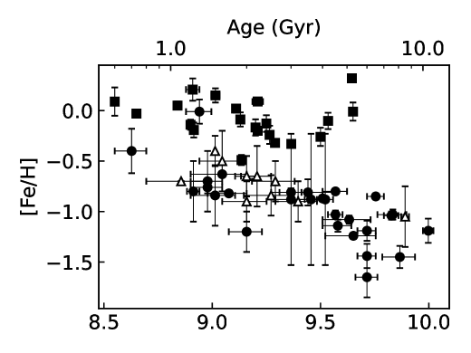
Figure 4: The age and metallicity of star clusters used to derive the absolute magnitude or colour of RC stars. Black circles are our SMC samples, black squares are our MW samples, and grey triangles are the samples of Onozato et al. (2019).

3.1.2 Milky Way star clusters

The absolute magnitude and colour of RC stars in star clusters containing a sufficient number of RC stars were determined using a method similar to that used for the SMC star clusters. The differences are as follows. First, we selected stars with $(DM-3.5)<m_{K_{S}}<(DM-0.5)$ and $0.4<J-K_{S}<1.0$ to derive the absolute magnitude and colour of the RC stars as shown in Figs. 5 and 6. Second, the members of the star clusters were selected based on the membership probability of Cantat-Gaudin & Anders (2020). We considered stars with a membership probability greater than 0.9 to be members of the star clusters, and we did not subtract field stars. For star clusters with fewer stars, the absolute magnitude and colour of RC stars were determined by calculating the average for stars within the same magnitude and colour range. Thus, the absolute magnitude and colour could be determined for the clusters studied by van Helshoecht & Groenewegen (2007) excluding NGC 2420 and NGC 6633, both of which contain only two RC stars. Only colour was used for Haffner 2, as its large DM of 15.512 mag (12.658 kpc) reduces the reliability of Gaia parallax measurements. A list of star clusters of this study is presented in Table 3.

Table 3: Milky Way Cluster Information

Cluster name	RA (J2000.0)	Dec (J2000.0)	Age ($\log t$)	[Fe/H]	$E(B-V)$	$DM$
NGC 188	00h 47m 11$\aas@@fstack{s}$52	+85°14′38$\aas@@fstack{\prime\prime}$4	9.650	$-0.010\pm 0.090$	0.085	$11.475\pm 0.009$
NGC 752	01h 56m 53$\aas@@fstack{s}$51	+37°47′38$\aas@@fstack{\prime\prime}$6	9.130	$-0.088\pm 0.070$	0.040	$8.250\pm 0.005$
NGC 1817	05h 12m 33$\aas@@fstack{s}$4	+16°41′46″	8.900	$-0.140\pm 0.050$	0.354	$11.294\pm 0.012$
M 37 (NGC 2099)	05h 52m 17$\aas@@fstack{s}$8	+32°32′42″	8.550	$0.089\pm 0.140$	0.350	$10.883\pm 0.007$
NGC 2204	06h 15m 31$\aas@@fstack{s}$7	-18°40′12″	$9.290\pm 0.018$	$-0.320\pm 0.100$	0.021	$13.399\pm 0.031$
NGC 2243	06h 29m 34$\aas@@fstack{s}$8	-31°16′55″	9.135	$-0.490\pm 0.050$	0.062	$13.379\pm 0.031$
Haffner 2 (Tombaugh 2)	07h 03m 05$\aas@@fstack{s}$5	-20°49′12″	9.010	$-0.310\pm 0.020$	0.354	$15.512\pm 0.165$
NGC 2360	07h 17m 46$\aas@@fstack{s}$3	-15°37′52″	$8.650\pm 0.018$	$-0.030\pm 0.010$	0.416	$10.884\pm 0.005$
Melotte 66	07h 26m 17$\aas@@fstack{s}$5	-47°41′06″	9.365	$-0.330\pm 0.030$	0.125	$13.688\pm 0.036$
Berkeley 39	07h 46m 48$\aas@@fstack{s}$5	-04°39′54″	9.500	$-0.260\pm 0.090$	0.042	$13.484\pm 0.054$
NGC 2477	07h 52m 11$\aas@@fstack{s}$0	-38°32′13″	$8.915\pm 0.007$	$-0.192\pm 0.074$	0.291	$10.886\pm 0.003$
NGC 2506	08h 00m 02$\aas@@fstack{s}$4	-10°46′23″	$9.210\pm 0.017$	$-0.200\pm 0.020$	0.042	$12.673\pm 0.015$
NGC 2527	08h 04m 59$\aas@@fstack{s}$0	-28°07′19$\aas@@fstack{\prime\prime}$2	$8.910\pm 0.031$	$-0.208\pm 0.110$	0.040	$9.068\pm 0.006$
NGC 2682	08h 51m 23$\aas@@fstack{s}$0	+11°48′50″	$9.535\pm 0.009$	$-0.102\pm 0.081$	0.050	$9.725\pm 0.004$
NGC 3680	11h 25m 34$\aas@@fstack{s}$1	-43°14′24″	9.200	$-0.167\pm 0.080$	0.062	$10.151\pm 0.010$
NGC 3960	11h 50m 34$\aas@@fstack{s}$6	-55°40′44″	9.110	$0.020\pm 0.040$	0.167	$11.990\pm 0.011$
NGC 5852	15h 04m 12$\aas@@fstack{s}$2	-54°21′58″	$8,840\pm 0.013$	$0.050\pm 0.040$	0.312	$9.628\pm 0.004$
NGC 6134	16h 27m 48$\aas@@fstack{s}$7	-49°09′40″	$9.015\pm 0.019$	$0.150\pm 0.070$	0.458	$10.363\pm 0.005$
IC 4651	17h 24m 50$\aas@@fstack{s}$9	-49°55′01″	9.250	$-0.128\pm 0.082$	0.121	$9.882\pm 0.004$
NGC 6791	19h 20m 53$\aas@@fstack{s}$0	+37°46′41″	9.645	$0.320\pm 0.020$	0.117	$13.583\pm 0.023$
NGC 6819	19h 41m 18$\aas@@fstack{s}$5	+40°11′24″	$9.210\pm 0.024$	$0.090\pm 0.030$	0.237	$12.243\pm 0.006$
NGC 7789	23h 57m 20$\aas@@fstack{s}$2	+56°43′34″	$9.265\pm 0.009$	$-0.240\pm 0.090$	0.237	$11.720\pm 0.005$

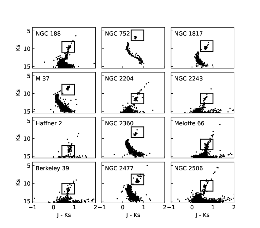
Figure 5: The same figure as Fig. 1 but for Milky Way star clusters.

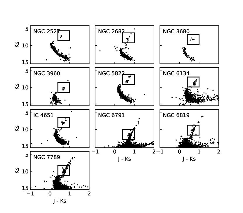
Figure 6: Continued from Fig. 5.

3.2 Multiple Regression Analysis

We performed a multiple regression analysis, following the method of Onozato et al. (2019) to confirm the population effects. This also enables correction for population effects when RC stars are used as a standard candle or crayon. The age range for the multiple regression analysis of absolute magnitude was restricted to 1–4 Gyr, as this range provided a sufficient sample size. The colour was analysed for the entire sample because the SMC dataset provided sufficient samples across the remaining range. To derive the correction formula, we performed least-squares fitting using the following function

$$M_{\lambda}=a(\log(t)-9.300)+b([\mathrm{Fe}/\mathrm{H}]+0.50)+c,$$ (4)

where $t$ represents the age (yr) of the star clusters. For colour, replace $M_{\lambda}$ with $m_{\lambda,\,1}-m_{\lambda,\,1}$.

4 Results and Discussion

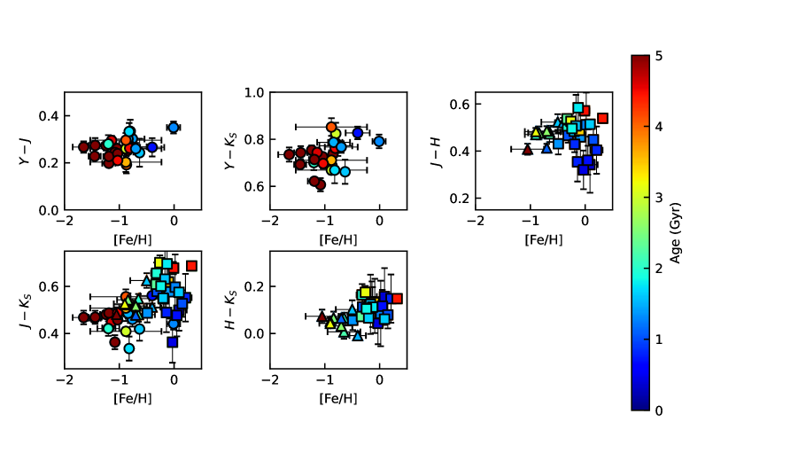
Figure 10: Mean RC colour versus metallicity in each cluster for $Y-J$ (upper left), $Y-K_{S}$ (upper centre), $J-H$ band (upper right), $J-K_{S}$ (lower left), and $H-K_{S}$ (lower centre). Colour scale represents age difference.

The derived absolute magnitude and intrinsic colour of RC stars in the star clusters are summarised in Tables 4 and 5. The absolute magnitude of the RC stars for each cluster, plotted against age and metallicity, are shown in Figs. 7 and 8, respectively. Figs. 9 and 10 depict the plots for colour.

Table 4: The derived RC colour of the SMC target star clusters.

Cluster name	$Y-J$	$Y-K_{S}$	$J-K_{S}$
Lindsay 1	$0.259\pm 0.007$	$0.726\pm 0.008$	$0.466\pm 0.008$
ESO 28-15	$0.244\pm 0.038$	$0.607\pm 0.028$	$0.362\pm 0.030$
ESO 28-17	$0.273\pm 0.021$	$0.753\pm 0.020$	$0.481\pm 0.018$
Lindsay 7	$0.302\pm 0.036$	$0.762\pm 0.033$	$0.460\pm 0.031$
ESO 28-19	$0.251\pm 0.013$	$0.737\pm 0.013$	$0.486\pm 0.012$
ESO 28-20	$0.243\pm 0.060$	$0.648\pm 0.051$	$0.405\pm 0.050$
NGC 121	$0.199\pm 0.013$	$0.622\pm 0.012$	$0.423\pm 0.012$
ESO 28-22	$0.274\pm 0.028$	$0.787\pm 0.031$	$0.513\pm 0.030$
NGC 152	$0.268\pm 0.015$	$0.772\pm 0.016$	$0.504\pm 0.015$
Lindsay 19	$0.193\pm 0.036$	$0.689\pm 0.037$	$0.496\pm 0.021$
Lindsay 27	$0.295\pm 0.019$	$0.744\pm 0.020$	$0.449\pm 0.019$
[RZ2005] 34	$0.266\pm 0.039$	$0.828\pm 0.027$	$0.562\pm 0.042$
Bruck 47	$0.350\pm 0.025$	$0.791\pm 0.029$	$0.441\pm 0.024$
ESO 51-3	$0.267\pm 0.024$	$0.735\pm 0.030$	$0.468\pm 0.029$
Kron 28	$0.280\pm 0.038$	$0.702\pm 0.032$	$0.421\pm 0.031$
NGC 339	$0.229\pm 0.011$	$0.714\pm 0.012$	$0.485\pm 0.011$
Kron 38	$0.280\pm 0.022$	$0.720\pm 0.019$	$0.440\pm 0.018$
[BS95] 90	$0.333\pm 0.048$	$0.823\pm 0.046$	$0.490\pm 0.045$
Kron 44	$0.262\pm 0.014$	$0.762\pm 0.013$	$0.500\pm 0.013$
NGC 361	$0.228\pm 0.016$	$0.692\pm 0.015$	$0.464\pm 0.011$
NGC 411	$0.300\pm 0.024$	$0.787\pm 0.024$	$0.487\pm 0.022$
NGC 416	$0.274\pm 0.031$	$0.743\pm 0.028$	$0.469\pm 0.028$
NGC 419	$0.254\pm 0.025$	$0.751\pm 0.025$	$0.497\pm 0.025$
[RZ2005] 194	$0.295\pm 0.030$	$0.852\pm 0.037$	$0.557\pm 0.031$
ESO 29-46	$0.203\pm 0.041$	$0.711\pm 0.042$	$0.508\pm 0.055$
ESO 29-48	$0.239\pm 0.029$	$0.699\pm 0.022$	$0.460\pm 0.025$
NGC 643	$0.333\pm 0.036$	$0.669\pm 0.056$	$0.336\pm 0.051$
Lindsay 113	$0.210\pm 0.013$	$0.698\pm 0.013$	$0.488\pm 0.012$

Table 5: The derived RC absolute magnitude and colour of the Milky Way target star clusters.

Cluster name	$M_{J}$	$M_{H}$	$M_{K_{S}}$	$J-H$	$J-K_{S}$	$H-K_{S}$
NGC 188	$-1.127\pm 0.017$	$-1.698\pm 0.016$	$-1.805\pm 0.023$	$0.571\pm 0.020$	$0.679\pm 0.026$	$0.108\pm 0.026$
NGC 752a	$-0.809\pm 0.080$	$-1.269\pm 0.082$	$-1.385\pm 0.081$	$0.460\pm 0.115$	$0.576\pm 0.114$	$0.116\pm 0.115$
NGC 1817	$-1.201\pm 0.059$	$-1.595\pm 0.063$	$-1.684\pm 0.065$	$0.394\pm 0.084$	$0.483\pm 0.086$	$0.089\pm 0.089$
M 37a	$-1.969\pm 0.060$	$-2.311\pm 0.104$	$-2.468\pm 0.063$	$0.342\pm 0.119$	$0.499\pm 0.086$	$0.157\pm 0.121$
NGC 2204	$-1.404\pm 0.045$	$-1.847\pm 0.034$	$-1.957\pm 0.034$	$0.443\pm 0.036$	$0.554\pm 0.035$	$0.111\pm 0.020$
NGC 2243	$-1.506\pm 0.044$	$-1.936\pm 0.045$	$-1.993\pm 0.040$	$0.431\pm 0.045$	$0.487\pm 0.040$	$0.057\pm 0.042$
Haffner 2	$-2.028\pm 0.166$	$-2.440\pm 0.167$	$-2.549\pm 0.167$	$0.411\pm 0.028$	$0.520\pm 0.035$	$0.109\pm 0.032$
NGC 2360	$-1.244\pm 0.058$	$-1.564\pm 0.059$	$-1.607\pm 0.066$	$0.320\pm 0.082$	$0.363\pm 0.087$	$0.043\pm 0.088$
Melotte 66	$-1.326\pm 0.043$	$-1.834\pm 0.038$	$-1.924\pm 0.038$	$0.508\pm 0.026$	$0.598\pm 0.028$	$0.090\pm 0.019$
Berkeley 39	$-1.275\pm 0.060$	$-1.801\pm 0.058$	$-1.976\pm 0.057$	$0.526\pm 0.032$	$0.701\pm 0.031$	$0.175\pm 0.027$
NGC 2477	$-0.943\pm 0.027$	$-1.392\pm 0.024$	$-1.494\pm 0.027$	$0.449\pm 0.036$	$0.551\pm 0.038$	$0.102\pm 0.036$
NGC 2506	$-1.222\pm 0.021$	$-1.721\pm 0.022$	$-1.790\pm 0.019$	$0.499\pm 0.021$	$0.568\pm 0.019$	$0.069\pm 0.019$
NGC 2527a	$-1.215\pm 0.070$	$-1.619\pm 0.072$	$-1.767\pm 0.074$	$0.404\pm 0.100$	$0.552\pm 0.102$	$0.148\pm 0.103$
NGC 2682a	$-1.119\pm 0.016$	$-1.607\pm 0.010$	$-1.738\pm 0.010$	$0.488\pm 0.018$	$0.619\pm 0.018$	$0.131\pm 0.013$
NGC 3680a	$-1.348\pm 0.097$	$-1.855\pm 0.090$	$-1.980\pm 0.090$	$0.507\pm 0.132$	$0.631\pm 0.132$	$0.124\pm 0.126$
NGC 3960a	$-1.050\pm 0.097$	$-1.562\pm 0.098$	$-1.647\pm 0.100$	$0.512\pm 0.136$	$0.597\pm 0.138$	$0.085\pm 0.139$
NGC 5822	$-1.050\pm 0.097$	$-1.562\pm 0.098$	$-1.647\pm 0.100$	$0.512\pm 0.136$	$0.597\pm 0.138$	$0.085\pm 0.139$
NGC 6134	$-0.981\pm 0.044$	$-1.331\pm 0.024$	$-1.498\pm 0.044$	$0.350\pm 0.049$	$0.517\pm 0.061$	$0.167\pm 0.049$
IC 4651	$-1.098\pm 0.048$	$-1.682\pm 0.062$	$-1.794\pm 0.059$	$0.584\pm 0.078$	$0.696\pm 0.076$	$0.112\pm 0.085$
NGC 6791	$-1.408\pm 0.013$	$-1.948\pm 0.026$	$-2.095\pm 0.025$	$0.540\pm 0.020$	$0.687\pm 0.017$	$0.148\pm 0.017$
NGC 6819	$-1.486\pm 0.013$	$-1.952\pm 0.019$	$-2.049\pm 0.015$	$0.466\pm 0.021$	$0.563\pm 0.018$	$0.097\pm 0.022$
NGC 7789	$-1.145\pm 0.020$	$-1.639\pm 0.020$	$-1.750\pm 0.021$	$0.493\pm 0.028$	$0.605\pm 0.028$	$0.111\pm 0.028$
a Clusters that simply adopt the average of the magnitude of RC candidate stars

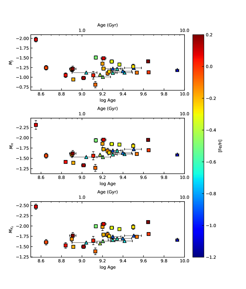
Figure 7: Mean RC absolute magnitude versus age in each cluster for $J$ (left), $H$ (centre), and $K_{S}$ band (right). Colour scale represents metallicity difference.

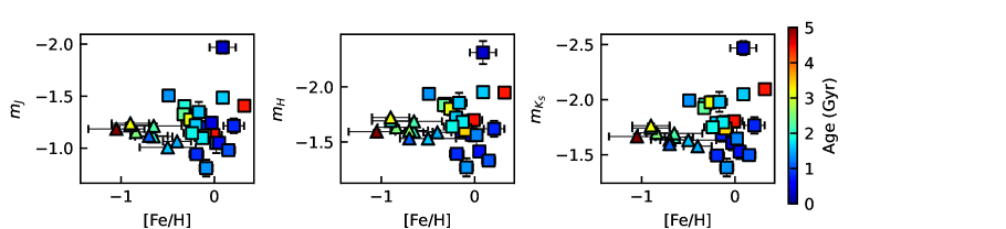
Figure 8: Mean RC absolute magnitude versus metallicity in each cluster for $J$ (left), $H$ (centre), and $K_{S}$ band (right). Colour scale represents age difference.

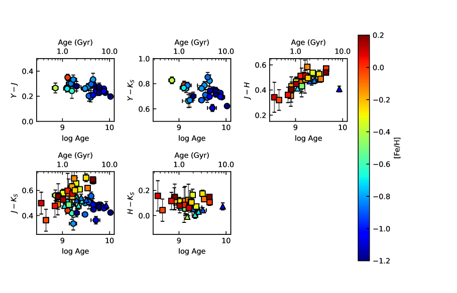
Figure 9: Mean RC colour versus age in each cluster for $Y-J$ (upper left), $Y-K_{S}$ (upper centre), $J-H$ band (upper right), $J-K_{S}$ (lower left), and $H-K_{S}$ (lower centre). Colour scale represents metallicity difference.

4.1 The Results of Multiple Regression Analysis

The following values were derived as the best fit results of absolute magnitude,

$$M_{J}=( -0.243\pm 0.200)(\log(t)-9.300)$$

$$-(0.012\pm 0.102)([\mathrm{Fe}/\mathrm{H}]+0.50)-(1.188\pm 0.038)$$ (5)

$$M_{H}=( -0.397\pm 0.198)(\log(t)-9.300)$$

$$-(0.038\pm 0.101)([\mathrm{Fe}/\mathrm{H}]+0.50)-(1.671\pm 0.038)$$ (6)

$$M_{K_{S}}=( -0.430\pm 0.197)(\log(t)-9.300)$$

$$-(0.129\pm 0.100)([\mathrm{Fe}/\mathrm{H}]+0.50)-(1.745\pm 0.038),$$ (7)

and colour,

$$Y-J=( -0.047\pm 0.033)(\log(t)-9.300)$$

$$+(0.014\pm 0.031)([\mathrm{Fe}/\mathrm{H}]+0.50)+(0.281\pm 0.012)$$ (8)

$$Y-K_{S}=( -0.044\pm 0.050)(\log(t)-9.300)$$

$$+(0.037\pm 0.048)([\mathrm{Fe}/\mathrm{H}]+0.50)+(0.759\pm 0.019)$$ (9)

$$J-H= (0.169\pm 0.033)(\log(t)-9.300)$$

$$+(0.053\pm 0.027)([\mathrm{Fe}/\mathrm{H}]+0.50)+(0.472\pm 0.010)$$ (10)

$$J-K_{S}= (0.122\pm 0.032)(\log(t)-9.300)$$

$$+(0.151\pm 0.023)([\mathrm{Fe}/\mathrm{H}]+0.50)+(0.525\pm 0.008)$$ (11)

$$H-K_{S}= (0.023\pm 0.027)(\log(t)-9.300)$$

$$+(0.076\pm 0.022)([\mathrm{Fe}/\mathrm{H}]+0.50)+(0.078\pm 0.008).$$ (12)

The equations derived for the absolute magnitude are compared for the four metallicities in Fig. 11 and for the colour in Fig. 12. We calculated the coefficients of determination to assess the goodness of fit. The coefficient of determination, adjusted for degrees of freedom (adjusted $R^{2}$), is given by

$$\mathrm{adjusted}\ R^{2}=1-\frac{\sum_{i}((M_{\lambda}-m_{\lambda,i})-f_{i})^{2}/(N-p-1)}{\sum_{i}(M_{\lambda,i}-\overline{M_{\lambda}})^{2}/(N-1)},$$ (13)

where $M_{\lambda}$ is the RC colour of observational data, $f$ is the colour from equations (5)–(7), $\overline{M_{\lambda}}$ is the average of $M_{\lambda}$, $N$ is the number of sample star clusters, and $p$ is the number of explanatory variables (three in this time). The calculated values of adjusted $R^{2}$ are 0.066, 0.165, and 0.234 for $M_{J}$, $M_{H}$, and $M_{K_{S}}$, respectively. These values are close to zero, indicating that the fitting results differ little from simply taking the average. The adjusted $R^{2}$ values for colour are 0.204, 0.165, 0.477, 0.433, and 0.306 for $Y-J$, $Y-K_{S}$, $J-H$, $J-K_{S}$, and $H-K_{S}$, respectively.

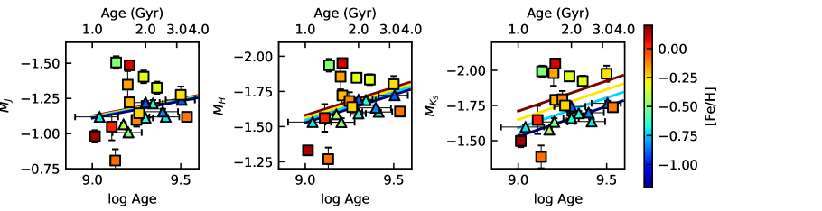
Figure 11: The same figure as Fig. 7 but with the best-fitting relations for four metallicities (from blue to brown, $-1.0$, $-0.67$, $-0.33$, $0.0$ dex).

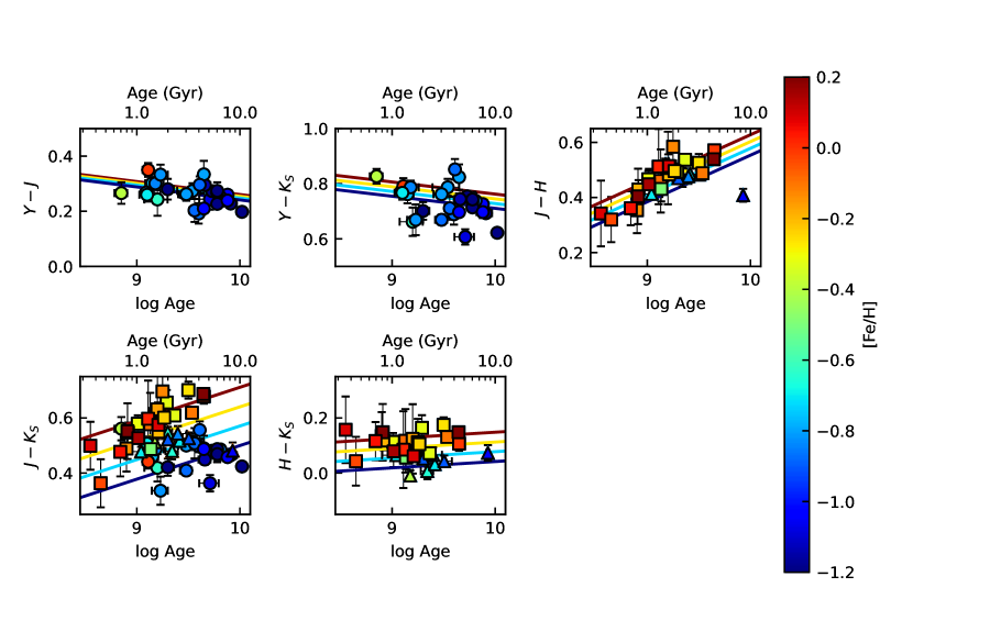
Figure 12: The same figure as Fig. 9 but with the best-fitting relations for four metallicities (from blue to brown, $-1.20$, $-0.73$, $-0.27$, $0.20$ dex).

4.2 Population effects

Multiple regression analysis indicates that the older RC stars are brighter in the 1–4 Gyr range for all $M_{J}$, $M_{H}$, and $M_{K_{S}}$, although the adjusted $R^{2}$ values are lower. This result is consistent with the LMC-only results of Onozato et al. (2019) and the theoretical predictions of Girardi (2016). The rapid brightening of the young RC with an age of 0.35 Gyr, although only in one cluster, is also in agreement with theoretical predictions.

Regarding the effect of metallicity on the NIR absolute magnitude of RC stars, no clear dependence has been confirmed. The best-fit results from the multiple regression analysis indicate brighter for higher metallicity within the 1–4 Gyr range for all $JHK_{S}$ bands, although the dependence is not significant when accounting for uncertainties. The weak metallicity dependence of the NIR absolute magnitude is consistent with observational results (Alves, 2000; Groenewegen, 2008; Laney et al., 2012) and theoretical predictions by Girardi (2016).

In terms of colour, $J-H$ and $J-K_{S}$ exhibit age dependence, with older RC stars appearing redder, whereas $Y-J$, $Y-K_{S}$, and $H-K_{S}$ do not show a strong dependence. Conversely, metallicity dependence indicates redder colour at higher metallicity for all colour, consistent with theoretical predictions, although the trend is weaker for $Y-J$ and $Y-K_{S}$. However, $Y-J$ and $Y-K_{S}$ data are available only for the SMC, and the trend may not be observed due to the limited age and metallicity range covered by these data. As shown in Fig. 4, the age-metallicity relationship is evident only the sample of the SMC clusters, where older star clusters have lower metallicity and younger star clusters have higher metallicity. The theoretical models predict that RC stars in the age range (0.5 $\lesssim$ age (Gyr) $\lesssim$ 8) become redder as they get older or have higher metallicity. In contrast, older RC stars are predicted to become bluer for young metal-rich RC stars (age $\lesssim$ 0.5  Gyr, [Fe/H] $\gtrsim$ 0.05) and old metal-poor RC stars (age $\gtrsim$ 8  Gyr, [Fe/H] $\lesssim$ -0.40). If samples from a single galaxy following the age-metallicity relation closely, the population effects are likely to cancel each other out. For $J-H$, the strong age dependence may result from the lack of SMC samples covering low-metallicity clusters.

4.3 Comparison with theoretical models

We compare the observed results not only with the model of Girardi (2016), but also with other theoretical models. We used three isochrone models for comparison: a Bag of Stellar Tracks and Isochrones (BaSTI, Pietrinferni et al., 2004), PARSEC version 1.2S evolutionary tracks (Bressan et al., 2012) and canonical two-part-power law IMF of Kroupa (2001, 2002), and MESA Isochrones & Stellar Tracks (MIST) version 1.2 (Paxton et al., 2011; Paxton et al., 2013, 2015, 2018; Dotter, 2016; Choi et al., 2016). Although other isochrone models are available, we used these models because they can perform calculations up to and beyond the helium burning stage, and they enable plotting isochrones across a wide range of age and metallicity. To define the mass range of RC stars in the isochrone models, we identify the region where the absolute magnitude remains nearly constant during the transition from the red giant branch (RGB) to the asymptotic giant branch. The lower mass boundaries of the RC stars are set at the minimum initial mass above the tip of the RGB for which the derivative of luminosity with respect to mass ($dL/dM$) becomes positive, indicating the beginning of a relatively flat luminosity region. The upper boundaries are defined as the lowest mass at which $dL/dM$ exceeds the mean value plus three times the standard deviation of $dL/dM$, evaluated over the interval from the lower boundary to a higher reference mass. This criterion provides a consistent and objective way to isolate the RC region from neighbouring evolutionary phases. The median absolute magnitude of stars within this mass interval is adopted as the representative RC magnitude for each age and metallicity in the models. Specifically, let $M_{1}$ be the minimum mass at which $dL/dM>0$ above the tip of the RGB, and $M_{2}$ the minimum mass satisfying $dL/dM>\langle dL/dM\rangle+3\sigma$ within $[M_{1},M_{\mathrm{ref}}]$; the RC magnitude is defined as the median absolute magnitude over [$M_{1}$, $M_{2}$].

No significant differences are observed in the trend of the population effect on absolute magnitude as shown in Fig. 13. When comparing absolute values, PARSEC appears to be slightly brighter. The population effect on RC colour shows little differences in trends between models. RC stars are commonly redder if they are older or more metal rich as depicted in Fig. 14. Additionally, the population effect is negligible for $H-K_{S}$. However, some differences are observed in the absolute values.

Figs. 15 through 17 compare the three models with our results for absolute magnitude, while Figs. 18 through 20 compare them for colour. The comparison results indicate that the age dependence is well reproduced. For colour, both the trends and absolute values show good agreement with observations and the models. In PARSEC, the model for metal-poor RC stars appears slightly bluer in $J-H$. The $H-K_{S}$ values deviate slightly due to the weak dependence, but they remain consistent within the range of observational uncertainties.

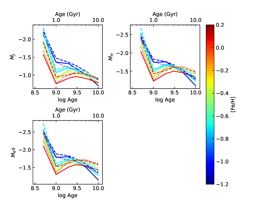
Figure 13: Comparison of the three isochrone models for four metallicities (from blue to brown, $-1.05$, $-0.70$, $-0.40$, $0.06$ dex). Solid lines are BaSTI, dashed lines are PARSEC, and dotted lines are MIST.

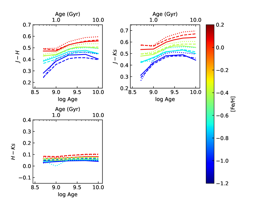
Figure 14: Comparison of the three isochrone models for four metallicities (from blue to brown, $-1.05$, $-0.70$, $-0.40$, $0.06$ dex). Solid lines are BaSTI, dashed lines are PARSEC, and dotted lines are MIST. Triangles are BaSTI, Circles are CMD 3.7, and Squares are MIST.

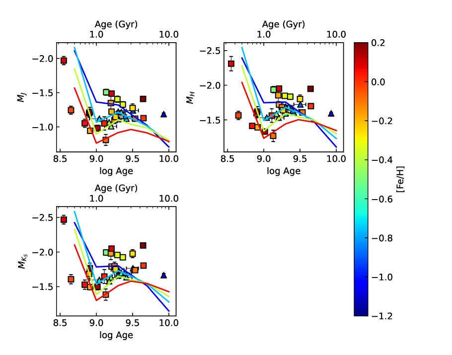
Figure 15: Comparison of absolute magnitude between the observed results and the BaSTI isochrone models for four metallicities (from blue to brown, $-1.05$, $-0.70$, $-0.40$, $0.06$ dex).

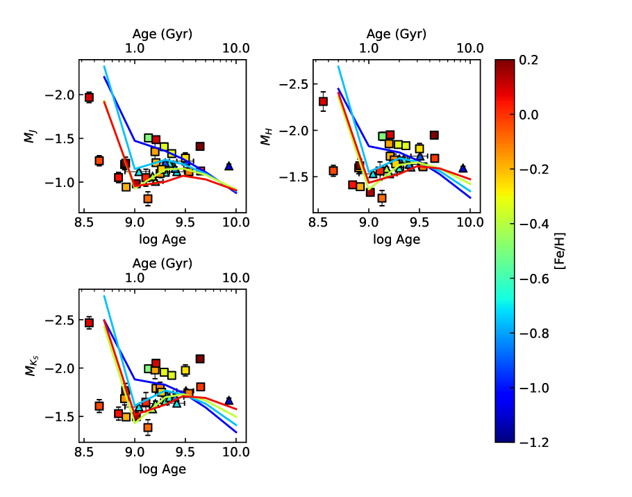
Figure 16: Comparison of absolute magnitude between the observed results and the PARSEC isochrone models for four metallicities (from blue to brown, $-1.05$, $-0.70$, $-0.40$, $0.06$ dex).

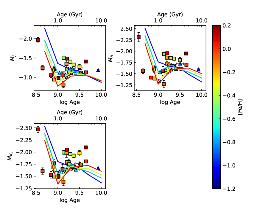
Figure 17: Comparison of absolute magnitude between the observed results and the MIST isochrone models for four metallicities (from blue to brown, $-1.05$, $-0.70$, $-0.40$, $0.06$ dex).

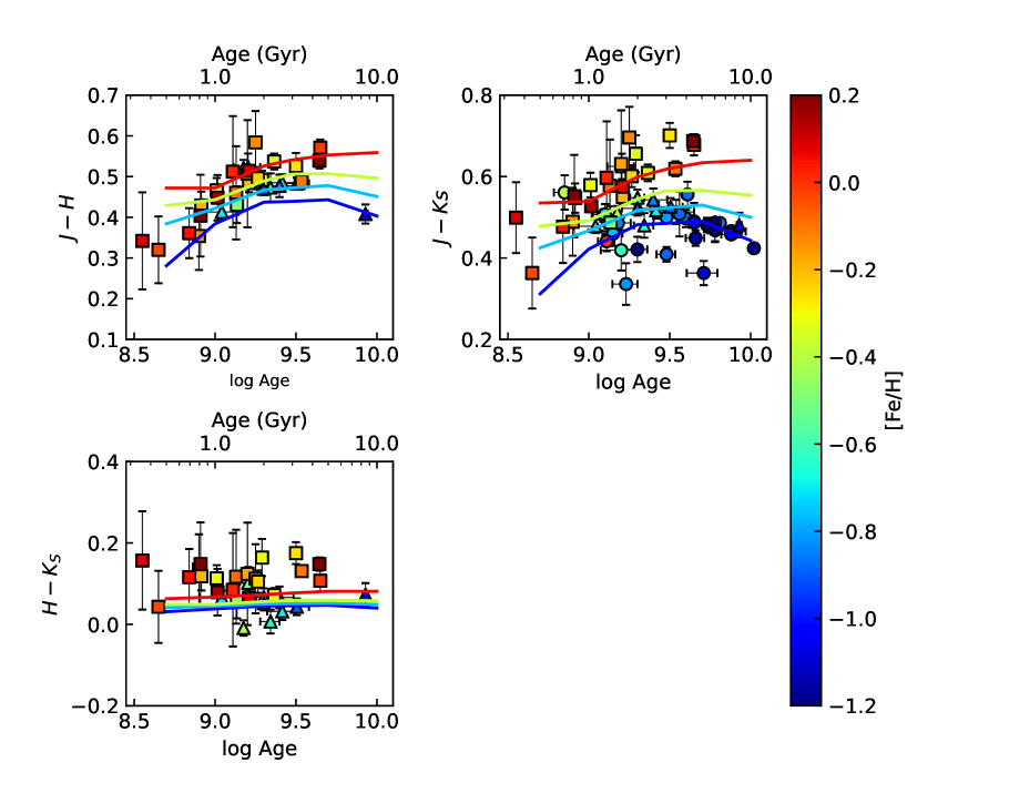
Figure 18: Comparison of colour between the observed results and the BaSTI isochrone models for four metallicities (from blue to brown, $-1.05$, $-0.70$, $-0.40$, $0.06$ dex).

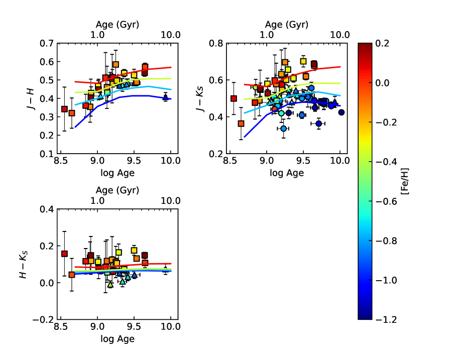
Figure 19: Comparison of colour between the observed results and the PARSEC isochrone models for four metallicities (from blue to brown, $-1.05$, $-0.70$, $-0.40$, $0.06$ dex).

Figure 20: Comparison of absolute magnitude between the observed results and the MIST isochrone models for four metallicities (from blue to brown, $-1.05$, $-0.70$, $-0.40$, $0.06$ dex).

4.4 Comparison with observational results in the solar neighbourhood

The mean absolute magnitude of RC stars in the solar neighbourhood is $M_{J}\sim-1.0$, $M_{H}\sim-1.5$, and $M_{K_{S}}\sim-1.6$ (Alves, 2000; Groenewegen, 2008; Laney et al., 2012; Ruiz-Dern et al., 2018; Plevne et al., 2020), although minor variations exist between studies. The simple averages of our results for target star clusters are $M_{J}=-1.190\pm 0.034$, $M_{H}=-1.678\pm 0.035$, and $M_{K_{S}}=-1.766\pm 0.037$, which are systematically brighter by 0.15–0.20 compared to the solar neighbourhood. One possible explanation for this discrepancy is the overestimation of distances derived from Gaia’s parallaxes for relatively distant star clusters in the Milky Way. For instance, Plevne et al. (2020) showed that the absolute magnitude of RC stars, determined by directly using the inverse of parallaxes as the distances, is about 0.10–0.15 mag brighter than that derived by adopting the results of Bailer-Jones et al. (2018), which used the galactic coordinates as a prior, considering the Galactic model. However, star clusters with brighter RC stars (NGC  2204, NGC  2243, NGC  6791, and NGC  6819) exhibit distances comparable to those obtained via isochrone fitting as employed by van Helshoecht & Groenewegen (2007), suggesting that the difference in absolute magnitude may arise from the population differences between the star clusters and the solar neighbourhood. As shown by the results of our results and as predicted by theory, the population effect on absolute magnitude is greater than the effect of age difference. Although the solar neighbourhood differs from star clusters in that it contains stars of various ages, it is possible to estimate the typical age from the absolute magnitude by assuming the metallicity. Applying the formula derived in this study to the absolute magnitude of the solar neighbourhood with [Fe/H] = 0, we obtain $\log(t)\sim 8.5$ in the $J$-band and $\log(t)\sim 8.8$ in the $H$- and $K_{S}$-bands. These values lie near the edge of the age range of the star clusters used for the fitting in this study suggesting that the local RC stars mainly originate from either younger or older populations. Expanding the age range of sample RC stars would be greatly facilitated if photometric data for extragalactic star clusters become available in the future. In addition, asteroseismology of the local RC stars is a promising approach to investigate their NIR brightness.

The average colour of RC stars in the solar neighbourhood is $J-H\sim 0.5$, $J-K_{S}\sim 0.6$, and $H-K_{s}\sim 0.1$, respectively. The simple averages of our results are $J-H=0.469\pm 0.011$, $J-K_{S}=0.517\pm 0.010$, and $H-K_{S}=0.092\pm 0.008$, which are bluer than the corresponding values for the solar neighbourhood for $J-H$ and $J-K_{S}$. When the samples are divided into RC stars from the Milky Way star clusters, the LMC star clusters and the SMC star clusters, $J-K_{S}$ is $0.577\pm 0.018$ in the Milky Way, $0.523\pm 0.014$ in the LMC and $0.468\pm 0.009$ in the SMC, respectively. This reflects population effects, especially for the metallicity dependence. The mean colour of the Milky Way star clusters, which have metallicity close to that of the Sun, is similar to the mean colour of the RC stars in the solar neighbourhood, while the mean colour of the SMC star clusters, which are dominated by low metallicity, is clearly bluer than those in the solar neighbourhood. This colour difference is consistent with the population effect trend identified in this study. On the other hand, the $H-K_{S}$ values are almost identical for both our samples and RC stars in the solar neighbourhood, which is also consistent with our results.

5 Conclusions

Using star clusters from the SMC and the Milky Way Galaxy, we investigate age and metallicity dependence of the absolute magnitude and colour of RC stars in the near-infrared within a previously unexplored parameter range. Multiple regression analysis was performed to examine the population effect on absolute magnitude. The results are consistent with the theoretical models, indicating that for RC stars in the 1-4 Gyr range, there is an age dependence with older RC stars being brighter, while the metallicity dependence is weak. For more accurate validation, particularly regarding the metallicity dependence, samples with precisely determined age, metallicity, and distance are required. Regarding colour, the trends for both age and metallicity align with those predicted by theoretical models. In particular, for $J-K_{S}$, the complete set of the LMC, the SMC and the Milky Way star cluster allowed us to extensively cover the parameter space, thus confirming both the age and metallicity dependence.

Data Availability

The PSF photometry data of the VMC survey is available from ESO Catalogue Facility (https://www.eso.org/qi/catalogQuery/index/340). The 2MASS photometry is available from NASA/IPAC Infrared Science Archive (https://irsa.ipac.caltech.edu/Missions/2mass.html).

References

- Alves (2000) Alves D. R., 2000, ApJ, 539, 732
- Alves & Sarajedini (1999) Alves D. R., Sarajedini A., 1999, ApJ, 511, 225
- Bailer-Jones et al. (2018) Bailer-Jones C. A. L., Rybizki J., Fouesneau M., Mantelet G., Andrae R., 2018, AJ, 156, 58
- Bica et al. (2020) Bica E., Westera P., Kerber L. d. O., Dias B., Maia F., Santos João F. C. J., Barbuy B., Oliveira R. A. P., 2020, AJ, 159, 82
- Bressan et al. (2012) Bressan A., Marigo P., Girardi L., Salasnich B., Dal Cero C., Rubele S., Nanni A., 2012, MNRAS, 427, 127
- Cantat-Gaudin & Anders (2020) Cantat-Gaudin T., Anders F., 2020, A&A, 633, A99
- Cardelli et al. (1989) Cardelli J. A., Clayton G. C., Mathis J. S., 1989, ApJ, 345, 245
- Chen et al. (2017) Chen Y. Q., Casagrande L., Zhao G., Bovy J., Silva Aguirre V., Zhao J. K., Jia Y. P., 2017, ApJ, 840, 77
- Choi et al. (2016) Choi J., Dotter A., Conroy C., Cantiello M., Paxton B., Johnson B. D., 2016, ApJ, 823, 102
- Cioni et al. (2011) Cioni M. R. L., et al., 2011, A&A, 527, A116
- Da Costa & Hatzidimitriou (1998) Da Costa G. S., Hatzidimitriou D., 1998, AJ, 115, 1934
- Da Costa & Mould (1986) Da Costa G. S., Mould J. R., 1986, ApJ, 305, 214
- Dalton et al. (2006) Dalton G. B., et al., 2006, in McLean I. S., Iye M., eds, Society of Photo-Optical Instrumentation Engineers (SPIE) Conference Series Vol. 6269, Society of Photo-Optical Instrumentation Engineers (SPIE) Conference Series. p. 62690X, doi:10.1117/12.670018
- Dias et al. (2016) Dias B., Kerber L., Barbuy B., Bica E., Ortolani S., 2016, A&A, 591, A11
- Dotter (2016) Dotter A., 2016, ApJS, 222, 8
- Emerson et al. (2006) Emerson J., McPherson A., Sutherland W., 2006, The Messenger, 126, 41
- Girardi (2016) Girardi L., 2016, ARA&A, 54, 95
- Girardi & Salaris (2001) Girardi L., Salaris M., 2001, MNRAS, 323, 109
- Glatt et al. (2008a) Glatt K., et al., 2008a, AJ, 135, 1106
- Glatt et al. (2008b) Glatt K., et al., 2008b, AJ, 136, 1703
- Grocholski & Sarajedini (2002) Grocholski A. J., Sarajedini A., 2002, AJ, 123, 1603
- Groenewegen (2008) Groenewegen M. A. T., 2008, A&A, 488, 935
- Kharchenko et al. (2013) Kharchenko N. V., Piskunov A. E., Schilbach E., Röser S., Scholz R. D., 2013, A&A, 558, A53
- Kroupa (2001) Kroupa P., 2001, MNRAS, 322, 231
- Kroupa (2002) Kroupa P., 2002, Science, 295, 82
- Laney et al. (2012) Laney C. D., Joner M. D., Pietrzyński G., 2012, MNRAS, 419, 1637
- Mighell et al. (1998) Mighell K. J., Sarajedini A., French R. S., 1998, AJ, 116, 2395
- Mould et al. (1992) Mould J. R., Jensen J. B., Da Costa G. S., 1992, ApJS, 82, 489
- Onozato et al. (2019) Onozato H., Ita Y., Nakada Y., Nishiyama S., 2019, MNRAS, 486, 5600
- Parisi et al. (2009) Parisi M. C., Grocholski A. J., Geisler D., Sarajedini A., Clariá J. J., 2009, AJ, 138, 517
- Parisi et al. (2014) Parisi M. C., et al., 2014, AJ, 147, 71
- Parisi et al. (2015) Parisi M. C., Geisler D., Clariá J. J., Villanova S., Marcionni N., Sarajedini A., Grocholski A. J., 2015, AJ, 149, 154
- Paxton et al. (2011) Paxton B., Bildsten L., Dotter A., Herwig F., Lesaffre P., Timmes F., 2011, ApJS, 192, 3
- Paxton et al. (2013) Paxton B., et al., 2013, ApJS, 208, 4
- Paxton et al. (2015) Paxton B., et al., 2015, ApJS, 220, 15
- Paxton et al. (2018) Paxton B., et al., 2018, ApJS, 234, 34
- Percival & Salaris (2003) Percival S. M., Salaris M., 2003, MNRAS, 343, 539
- Perren et al. (2017) Perren G. I., Piatti A. E., Vázquez R. A., 2017, A&A, 602, A89
- Piatti (2011a) Piatti A. E., 2011a, MNRAS, 416, L89
- Piatti (2011b) Piatti A. E., 2011b, MNRAS, 418, L69
- Piatti et al. (2001) Piatti A. E., Santos J. F. C., Clariá J. J., Bica E., Sarajedini A., Geisler D., 2001, MNRAS, 325, 792
- Piatti et al. (2005a) Piatti A. E., Sarajedini A., Geisler D., Seguel J., Clark D., 2005a, MNRAS, 358, 1215
- Piatti et al. (2005b) Piatti A. E., Santos J. F. C. J., Clariá J. J., Bica E., Ahumada A. V., Parisi M. C., 2005b, A&A, 440, 111
- Piatti et al. (2007a) Piatti A. E., Sarajedini A., Geisler D., Gallart C., Wischnjewsky M., 2007a, MNRAS, 381, L84
- Piatti et al. (2007b) Piatti A. E., Sarajedini A., Geisler D., Gallart C., Wischnjewsky M., 2007b, MNRAS, 382, 1203
- Piatti et al. (2011) Piatti A. E., Clariá J. J., Bica E., Geisler D., Ahumada A. V., Girardi L., 2011, MNRAS, 417, 1559
- Piatti et al. (2015) Piatti A. E., de Grijs R., Rubele S., Cioni M.-R. L., Ripepi V., Kerber L., 2015, MNRAS, 450, 552
- Pietrinferni et al. (2004) Pietrinferni A., Cassisi S., Salaris M., Castelli F., 2004, ApJ, 612, 168
- Plevne et al. (2020) Plevne O., Önal Taş Ö., Bilir S., Seabroke G. M., 2020, ApJ, 893, 108
- Rochau et al. (2007) Rochau B., Gouliermis D. A., Brandner W., Dolphin A. E., Henning T., 2007, ApJ, 664, 322
- Ruiz-Dern et al. (2018) Ruiz-Dern L., Babusiaux C., Arenou F., Turon C., Lallement R., 2018, A&A, 609, A116
- Sabbi et al. (2007) Sabbi E., et al., 2007, AJ, 133, 44
- Salaris & Girardi (2002) Salaris M., Girardi L., 2002, MNRAS, 337, 332
- Skrutskie et al. (2006) Skrutskie M. F., et al., 2006, AJ, 131, 1163
- de Freitas Pacheco et al. (1998) de Freitas Pacheco J. A., Barbuy B., Idiart T., 1998, A&A, 332, 19
- van Helshoecht & Groenewegen (2007) van Helshoecht V., Groenewegen M. A. T., 2007, A&A, 463, 559