The foundational value of quantum computing for classical fluids

Abstract

Quantum algorithms for classical physics problems expose new patterns of quantum information flow as compared to the many-body Schrödinger equation. As a result, besides their potential practical applications, they also offer a valuable theoretical and computational framework to elucidate the foundations of quantum mechanics, particularly the validity of the many-body Schrödinger equation in the limit of large number of particles, on the order of the Avogadro number. This idea is illustrated by means of a concrete example, the Block-Encoded Carleman embedding of the Lattice Boltzmann formulation of fluid dynamics (CLB).

I Introduction

In his Nobel speech, Walter Kohn argued that the N-body Schrödinger equation (NBSE) is unlikely to bear any physical meaning beyond $N\sim 100$ [1]. The statement stems from the exponential amount of information contained in the $N$-body Hilbert space, in a $d$-dimensional grid with $g$ collocation points per dimension, the number of degrees of freedom scales like $g^{dN}$, the usual curse of dimensionality problem. This observation was made precise in by Poulin et al., who showed that physical time evolution can only explore a tiny fraction of the available Hilbert space [2].

Kohn and Poulin’s arguments raise a far-reaching question for quantum information science, namely whether the flow of quantum information in macroscopic systems, with $N$ of the order of the Avogadro number, can be organized according to patterns other than the NBSE. In this Letter, it is argued that quantum computing for classical systems provides a concrete framework to seek operational answers to this basic question.

As famously proclaimed by Feynman in his trailblazing 1982 paper [3], Nature isn’t classical, hence if we wish to simulate Nature, we’d better make it on quantum computers. Feynman was less explicit on the fact that even though Nature is quantum, it has a nearly unstoppable built-in tendency to become classical at sufficiently large scale and/or high temperatures. He implicitly recognized this by adding that the problem is interesting because it is not easy at all, classicalization being precisely the reason which makes quantum computing so hard to realize in practice. The fight against classicalization through noise mitigation and quantum error correction is a mainstay of current quantum computing research, but in this Perspective we address a different question, namely whether a classical system can be simulated according to quantum mechanical rules (not necessarily NBSE) and possibly faster than on a classical computer.

In principle the first part of this question may seem circular; given that the world is quantum mechanical, and classical physics emerges from quantum mechanics, at the fundamental level, any classical system must be implicitly computed quantum mechanically. This assumes that Nature can afford the luxury of computing all the way in Hilbert space, wasting most of its marbles on empty regions, while classical physics emerges through non-unitary dynamics such as decoherence and/or measurement. On closer inspection, however, the question is far from empty, because there might exist quantum algorithms for the simulation of classical physics which are not based on the emergence of classicality from the NBSE. Assessing the existence of such algorithms is conceptually important because it offers concrete alternatives to the $N$-body Schrödinger equation for macroscopic matter, thereby putting flesh into Kohn’s speculations. Whether they can outdo their classical counterparts is a separate and much more difficult question, which we also address in this Letter.

We investigate these matters by means of a concrete example, the formulation of a quantum Carleman-Lattice Boltzmann algorithm for classical fluids. Before dwelling into the details of this specific approach, let us summarize the main guidelines of the general framework such specific method belongs to.

i) Discretization: we ultimately aim at concrete quantum simulations, hence we consistently deal with large but finite numbers of degrees of freedom.

ii) Uplifting: classical systems are typically dissipative, meaning that they leak information to the surrounding environment in an irreversible way. Reversibility can be restored by enlarging the state space so as to include extra-degrees of freedom (environment) absorbing the information lost by the system, so that the System+Environment (Universe) is reversible and can consequently be described by a unitary dynamics.

iii) Linear Embedding: classical systems are most often nonlinear, hence incompatible with the quantum superposition principle which lies at the roots of quantum computing. The nonlinearity can be traded for extra-dimensions via linear embedding of the dynamics into infinite-dimensional spaces and then truncated to a finite order (see point 1).

iv) Nonlinear Depletion: The truncation order is strictly related to the strength of the nonlinearity, whence the scope for formulations which present the least nonlinear strength. Several techniques are known in theoretical physics to weaken the nonlinear coupling, renormalization group techniques and AdS-CFT duality being two prominent examples in point [4, 5]. In our case, this is achieved by simply moving to a phase-space representation of the system, i.e. the Boltzmann kinetic level [6].

v) Quantum Simulation: the final goal of the program is not only to provide complexity estimates but to deliver a concrete quantum algorithm and associated quantum circuit to be simulated on actual quantum hardware.

Progress on all these steps i-iv has been made in a number of disconnected works. Reversible microscopic models such as the hydrodynamic lattice-gas automata are a form of both discretization and uplifting - replacing irreversible nonlinear fluid dynamics by reversible nonlinear dynamics of particles on a lattice [7]. Other approaches to uplifting fluid equations to make them Hamiltonian, and hence reversible, have been given in [8]. Linearization is the basis for many current quantum approaches to nonlinear differential equations, including Carleman approaches [9, 10] discussed here but also “replica” methods based on linear evolution of many copies of the system [11]. Renormalization techniques for partial differential equations are well established [4, 12] and of current interest [13]. Techniques for reducing nonlinearities in field theories by similarity renormalization have also been applied to fluid equations in [14]. In this article we argue that quantum algorithms for fluid dynamics require further progress in all steps, and raises interesting foundational questions about the emergence of nonlinearity and the transition to classicality. Having clarified the conceptual framework, a few general comments on quantum computing for fluids are now in order.

II Quantum computing for fluids

Quantum computing emanates from two basic properties of quantum mechanics: Linearity and Unitarity [15, 16]. The physics of fluids is generally neither, hence the solution of the fluid equations on quantum computers immediately faces two major obstacles: Nonlinearity and Dissipation [17]. In the following we present one out of many possible strategies around both obstacles: Carleman embedding combined with block-encoding of sparse matrices.

II.1 Dealing with non-linearity: Carleman embedding

Carleman embedding is an uplifting technique whereby a finite-dimensional non linear system is formally turned into an infinite-dimensional linear one [18]. Hence, the basic idea is to trade nonlinearity for infinite-dimensionality.

As an elementary and yet representative example, let us consider the logistic equation

$$\dot{x}=-ax+bx^{2}$$ (1)

with initial condition $x(0)=x_{0}$ and $a,b>0$. The coefficient $a$ mimics dissipation while the ratio $R=b/a$ measures the strength of the quadratic nonlinearity versus dissipation, the ”analogue” of the Reynolds number in actual fluids (which also feature a quadratic nonlinearity). The logistic dynamics shows two attractors, a stable one at $x_{S}=0$ and an unstable one at $x_{U}=1/R$. This means that any initial condition below $1/R$ decays asymptotically to zero, while for $x_{0}>1/R$, the solution exhibits a finite-time singularity at $t=t^{*}=a^{-1}\log(\frac{r}{r-1})$, as it is apparent from the analytical solution

$$x(t)=x_{0}\frac{e^{-at}}{1-r+re^{-at}}$$

where we have set $r=Rx_{0}$. Initially, this solution decays as $e^{-at}$, as long as $|r(e^{-at}-1)|\ll 1$, followed by a slower decay but still converging to zero as $\frac{e^{-at}}{1-r}$, provided $r<1$, see Fig. 1.

Figure 1: The converging (blue solid line) and the diverging (red solid line) solutions of the logistic equation, obtained by setting the initial condition smaller, $x_{0}=0.5$, and larger, $x_{0}=2$, than $1/R$ respectively, with $R=1.5$ (black dashed horizontal line). The gray vertical line marks the time singularity for the unstable solution $t^{*}$.

Carleman embedding sets out to capture this multi-timescale relaxation through the progressive insertion of extra-variables, each describing an increasingly longer time scale.

In practice, upon letting $x_{1}\equiv x$ and $x_{2}\equiv x^{2}$, the logistic equation rewrites as

$$\dot{x}_{1}=-ax_{1}+bx_{2}$$

This is linear, but open, since $x_{2}$ is formally a new unknown. The equation for $x_{2}$ is readily derived

$$\dot{x}_{2}=2x\dot{x}=-2ax^{2}+2bx^{3}\equiv-2(ax_{2}-bx_{3})$$

The name of the game is quite clear, the embedding

$$x\to\{x_{k}\equiv x^{k}\},\;k=1,k_{max}$$

turns the original nonlinear problem into an infinite hierarchy

$$\dot{x}_{k}=-k(ax_{k}-bx_{k+1})$$

Occasionally, this linear hierarchy of ODE’s can be integrated analytically in the limit $k_{max}\to\infty$, thereby recovering the exact solution. More typically, the hierarchy is truncated at a given level $k_{max}$ by setting $x_{k_{max}+1}=0$, thereby providing a closed approximated solution to the nonlinear problem. In Fig. 2 we show the approximate curves at increasing values of $k_{max}$ for the stable solution with $x_{0}<1/R.$

Figure 2: The analytical solution of the logistic equation in the stable regime (blue solid line) is compared with the solutions of the Carleman system of equations with increasing truncation order $k_{max}$, which yields a better approximation of the solution. We set $x_{0}=0.5$ and $R=1.5$, hence $r=3/4$.

The basic idea is that low order truncations may offer cheap approximations within a finite time interval $0<t<t_{max}$. On intuitive grounds, one expects that at a given level of accuracy $\epsilon_{k}(t)=|x(t)-x_{k}(t)|$ at given time $t$ and for a defined truncation cutoff $k_{max}$, the latter should be an increasing function of $R$. The specific shape of this function dictates whether or not trading non-linearity for higher-dimensionality is a good bargain. In Figure 3 we show how the error $\epsilon_{k}(t)$ changes with the non-linearity parameter $R$. The same level for $\epsilon$ is reached at larger $k_{max}$ when $R$ increases.

Figure 3: The accuracy $\epsilon_{k}(t)$ calculated at $t=2$ for given $k_{max}=1$ (red dashed line), $k_{max}=2$ (green dotted line) and $k_{max}=3$ (purple solid line). The initial condition is set to $x_{0}=0.5$, therefore the stable region is $0<R<2$.

This is made clear in Fig. 4, where we show the minimum cutoff $k_{min}(R,\epsilon)$ that one should use to solve the logistic equation with fixed accuracy, for a given nonlinearity $R.$

Figure 4: The minimum value $k$ of the truncation order $k_{max}$ to achieve accuracy $\epsilon$ for given nonlinearity $R$. $\epsilon$ is calculated at time $t=2$ and represented in log scale, while the initial condition is set to $x_{0}=0.5$ and defines the stable region $0<R<2$. The isolines for $k$ are drawn in white.

On classical computers, Carleman linearization can be solved by a number of techniques, but does not seem to have gained any prominent role. On quantum computers, it provides an elegant and appealing strategy to eliminate nonlinearity. This does not come for free, since a Carleman scheme on a grid with $G$ grid points and $k$ levels of approximation takes about

$$N_{C}\sim G^{k}$$ (2)

variables, hence a very large matrix problem.

Carleman linearization for quantum simulations was first applied to the Burgers equation with encouraging results [9]. However the Burgers equation, besides being one-dimensional, is also pressure-free which is a drastic simplification of the physics of fluids. Subsequent application to the two-dimensional Navier-Stokes equations [19] has shown very poor convergence, mostly on account of the non-local coupling between the flow and pressure fields. However, once applied to the lattice Boltzmann formulation [21, 20] of fluid dynamics, it has shown extremely encouraging results, with errors around $\epsilon\sim 10^{-4}$ for hundreds of time-steps even at the lowest rung of the Carleman ladder, namely $k_{max}=2$. The reasons for this excellent performance have been discussed at length in the original papers, but essentially they amount to the fact that the nonlinearity in the dynamic of phase-space fluids is controlled by the Mach number (typically order 1) instead of the Reynolds number (typically order millions and billions). Moreover, the free-streaming operator is exact and unitary.

Unfortunately, these excellent properties are not sufficient to deliver an efficient quantum algorithm, the main problem being that the Carleman LB matrix projects upon virtually all of the tensor Pauli basis matrices. Symbolically, upon expanding the Carleman matrix onto the tensor Pauli basis $P_{l}$, $C_{ij}=\sum_{l=1}^{N_{c}}c_{l}P^{(l)}_{ij}$, it is found that the coefficients scale like $|c_{l}|\sim 1/l$. This means that none of them can be ignored and the depth of the resulting quantum circuit scales like $N_{c}^{2}=2^{2q}$,like a random unitary.

This discomforting outcome can be circumvented by moving to a sparse-matrix representation of the Carleman matrix, whereas each non-zero element $c_{ij}$ is representd by two types of oracles, one providing the locations $j=1,2\dots s$ ($s$ is the sparsity of the Carleman matrix) such that $c_{ij}\neq 0$, and the other providing the non-zero values $c_{ij}$ themselves. The number of ancilla qubits is fixed by the sparsity of the Carleman matrix $q_{a}\sim log_{2}s$. The explicit form of these oracles has been worked out and shown to bring the exponential depth down to a quadratic one. The interested reader is kindly directed to the original literature [10, 20, 22].

Yet, this leaves us with another problem, namely the fact that the implementation of the oracles requires extra qubits, known as ancillas, which in turn imply a non-zero failure rate of the quantum update, an issue that we are going to discuss in the next section.

II.2 Dealing with dissipation: Block Encoding

Next, we address the second obstacle: non-unitarity. A number of strategies are available to turn a dissipative system into a conservative one, but the most popular one is the so called Block-Encoding (BE), whereby the quantum system mapped into the state $|\psi\rangle$ of $q_{s}$ qubits is augmented with a number $q_{a}$ of auxiliary qubits known as ”ancillas” $|a\rangle$, representing the environment [23]. The enlarged state $|\Phi\rangle\equiv|\psi\rangle|a\rangle$ is acted upon by a correspondingly augmented Carleman operator $\hat{C}_{BE}$, such that the BE update formally reads as follows:

$$\dot{f}=C_{BE}f$$ (3)

where $f$ is the set of Carleman variables at a given truncation level $k$. For instance in the case $k=2$ this is the set of one and two-body distributions $f=\{f_{i}(x_{1}),f_{ij}(x_{1},x_{2})\}$, where $x_{1}$ and $x_{2}$ are spatial coordinates and the subscripts $i,j$ label the discrete velocities. The embedding of this classical two-body problem into a quantum representation is described in the original papers [20].

A schematic quantum circuit is shown in Fig 5. It is easy to show that this update recovers the original and correct one only whenever all the ancilla qubits are aligned in state $|0\rangle$, in which case they do not ”contaminate” the update. The upper bound for this to happen can be estimated as $p_{a}\sim 2^{-2q_{a}}$, highlighting a severe constraint at increasing number of ancilla qubit..

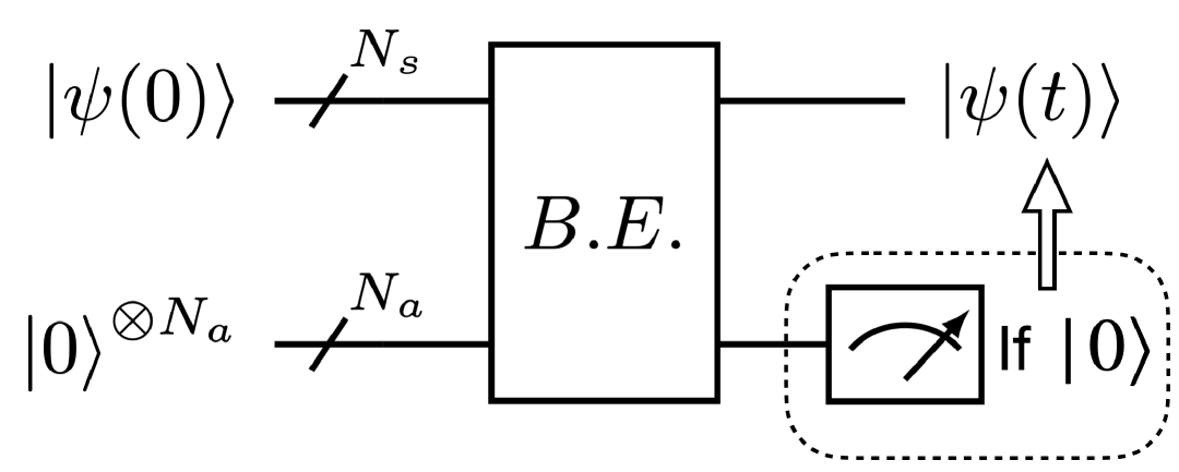
Figure 5: The quantum circuit for block encoding a nonunitary operation into the unitary operator B.E. The success of the algorithm is conditioned on measuring all the $q_{a}$ ancilla qubits in the state $|0\rangle$. This happens with a probability $p\sim 2^{-2q_{a}}$, with little dependence upon the number of system qubits $q_{s}.$

Block-Encoded Carleman-LB (BECLB) algorithms have been developed in the last few years, the bottom line being that the corresponding circuits offer a favorable (quadratic) scaling of the circuit depth with the number of qubits [22]. However, the success probability of the dissipative update is pretty low, of the order of $10^{-4}$ for a single time-step, thus compromising the viability of multi-step integration. A possible way out is offered by telescopic quantum algorithms, whereby the solution at a given finite time $t$ is reached within only a few timesteps, ideally just one, so as to curb the effects of low success probability. Again, the detail-thirsty reader is kindly directed to the original literature [24, 25].

Next we reconnect with the main theme of this paper, namely the foundational value of quantum algorithms as ”alternatives” to the NBSE equation in the limit $N\to\mathcal{A}$, the Avogadro number.

III Quantum lessons from the water faucet

For the sake of concreteness we refer to the simulation of the very ordinary case of fluid physics: the water flow from a kitchen faucet. The reason is that such flow is within grasp of current BECLB algorithms [20].

Let us recall that the number of active dynamic degrees of freedom (”eddies”) in a fluid over a time span $t\sim L/U\sim G^{1/3}$ is given by [26]:

$$N_{dof}=Re^{3}$$

where $Re=UL/\nu$ is the Reynolds number, $U$ being the flow speed, $L$ a typical macroscale and $\nu$ is the kinematic viscosity. For a water faucet, $U=1$ ($m/s$), $L=0.01$ ($m$) and $\nu=10^{-6}$ ($m^{2}/s$), so that $Re\sim 10^{4}$ and $G=10^{9}$. The number of floating point operations required to complete a dynamic simulation over a time span $t\sim L/U$ is approximately $10^{3}Re^{3}\sim 10^{15}$, meaning that a mid-end Teraflops/s computer can simulate this flow in about one hour wall clock time. This is where classical computing for classical fluids (CC) stands today [27].

Next, let us address the other extreme, the same flow taken head-on via the NBSE. A centimeter cube of water contains about $10^{22}$ molecules, which we equate for simplicity to the Avogadro number $\mathcal{A}\sim 6\times 10^{23}$. This is basically the number of dimensions of Hilbert space underneath the humble faucet flow. With a modest $g=10$ grid points per dimension, this leads to $G_{NBSE}\sim g^{\mathcal{A}}$ grid points, to be compared with the $G_{NS}=Re^{9/4}=10^{9}$ grid points required by the solution of the Navier-Stokes equations on a classical computer: Kohn’s point in full glory.

How about quantum computers? Assuming a perfect logarithmic scaling, we are left with the order of $\mathcal{A}$ qubits, still completely undoable for any foreseeable quantum computer and astronomically more costly than the classical simulation.

The question comes back again: Nature is hierarchical and modular, in that at each level offers ”effective” descriptions based on the relevant degrees of freedom of that specific level.

In our case, a single fluid degree of freedom (”eddy”) contains about $\mathcal{A}/G_{NS}=10^{14}$ molecules, this is the information compression associated with the passage from the Schroedinger to the Navier-Stokes levels.

If we insist that Nature, being quantum, must necessarily compute according to quantum mechanics, we come to the rather puzzling conclusion that Nature, as an analogue quantum computer, ignores the perks offered by its own ”emergent” properties.

Three options then arise, one bad, one good and one golden.

1) The bad: Nature is a super-powerful analogue quantum computer and as a such, it can afford the luxury of computing quantum mechanically all the way, according to the NBSE. If so, Kohn’s argument does not apply: we can’t compute with NBSE but Nature can.

2) The good: There are ways of computing macroscopic classical systems according to quantum mechanics (linear and unitary) on different and more economic grounds than the NBSE, yet less efficient than classical fluid solver. This has significant foundational value because it points to concrete alternatives to the NBSE, e.g. in our case the equation (3). Kohn is right, but this has no practical impact on the use of quantum computers for fluids.

3) The golden: Quantum algorithms are not only faster than the NBSE but also than classical computers. Besides the foundational value, this would mark a major practical breakthrough.

It is easy to see that the positioning of CLB is crucially dependent on the single-step success probability. A CLB² (CLB truncated at second order) features about $G^{2}$ Carleman variables, hence $10^{18}$ for the water faucet, corresponding to approximately $18log_{2}10\sim 60$ physical qubits in an ideal quantum-computing world with perfect error-correction algorithms.

This is astronomically less than the Avogadro-like number of qubits required by NBSE. However, with probability of success of the order of $10^{-4}$ a $10^{3}$ step simulation succeds in reproducing the correct quantum state with a probability $10^{-4000}$, which completely defeats the purpose of CLB (making it much worst than NBSE).

As mentioned earlier on, a possible way out is to develop telescopic algorithms capable of reaching the final state in a handful of time-steps, ideally just one. Roughly speaking, to bridge the gap with classical computing (on the optimistic assumption that the quantum clock ticks at the same rate as classical ones), one would need to meet the following condition: $60$ qubits with $p$ wins over $10^{9}$ grid sites provided

$$60/p<10^{9}.$$

This means one step with $p_{1}=60/10^{9}\sim 10^{-7}$, two steps with $p_{1}=10^{-3.5}$ and so on.

More generally, a BECLB update with $k$ Carleman levels, $T$ timesteps and a single-step success probability $p$, wins over the classical simulation on a grid with $G$ grid ponts, provided $p^{T}>\frac{klogG}{G},$ namely:

$$p>p_{min}(G,T;k)=\left(\frac{klogG}{G}\right)^{1/T}$$ (4)

The value of the minimum success probability (MSP) $p_{min}$ as a function of $G$ and $T$ is plotted in Figure 6 for the case $k=2$. From this figure it is clear that in order to compete with classical simulations, the BECLB procedure must feature nearly perfect success probabilities, unless an extremely efficient telescopic version can be developed. In the latter case, a ten-step telescopic algorithm would be competitive at a comparatively low success probability $p_{min}\sim 0.18$, three orders of magnitude above the current values. And the ideal case, $T=1$, would work with $p_{min}\sim 10^{-7}$.

IV From water faucets to numerical weather forecast

The previous section dealt with the ”mundane” case of the water faucet because the corresponding Reynolds number is in the range of what can be achieved by emulating CLB on present-day classical computers. However, the real breakthrough would be to perform fluid simulations which exceed the capabilities of foreseeable classical computers. A prominent example in point is numerical weather forecast [28]. The Reynolds number associated to the global atmospheric circulation is of the order of $Re\sim 10^{12}$, which implies $G\sim 10^{27}$ grid points and roughly $10^{40}$ floating point operations for a simulation of $T\sim G^{1/3}=10^{9}$ time-steps. These numbers speak for themselves as to the impossibility of any foreseeable classical computer to come any near to such target.

On the strong assumption that CLB can still compute within a few Carleman iterates because the nonlinearity is controlled by Mach and not Reynolds, the MSP for such calculation is $p_{min}(G=10^{27},T=10^{9},k=2)\sim 0.99999994$ namely a maximum failure rate $f_{max}=1-p_{min}\sim 5\;10^{-8}$, i.e. 50 parts per billion. This is extremely small, and yet higher than the failure rate of single base DNA replication (after proof-reading and post-replication mismatch repair), about one in ten billions. Hence, even discarding tomographic costs, succesfull quantum computing for numerical weather forecast requires genetic accuracy! Unfortunately, this is not compatible with the constraints set by the ancillas, $p_{max}\leq 2^{-2q_{a}}$, hence telescopic versions are a must.

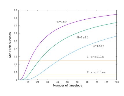
Figure 6: The minimum success probability as a function of the number of time steps for three representative grid sizes $G=10^{9}$ (water faucet), $G=10^{15}$ (full airliner), $G=10^{27}$ (global weather forecasting. The horizontal bars correspond to the maximum value allowed by the number of ancilla qubits. The crossing between the curves and the horizontal lines defines the maximum number of timesteps above which quantum advantage is lost (The figure does not account for tomographic costs of reconstructing the state after copying to proceed to the next step). Note that even though the number of time steps $M$ grows with increasing grid size, the effect is illusory when measured in terms of the classical number of steps $G^{1/3}$. This largely offsets the benefits of the $(klogG)/G$ reduction.

The figure clearly shows that once the ancilla barrier is accounted for, the quantum time marching should not employ more than a few ten steps at most. This is an extremely severe constraint, especially if measured in natural units of the $G^{1/3}$ steps required by the classical simulation. The problem of low success rates is currently being addressed via extensions of the oblivious amplitude amplification method to non-unitary matrices [29].

Summarizing, we have discussed three approaches, N-body schroedinger (NBSE), Carleman Lattice Boltzmann (CLB) and classical Navier-Stokes (NS).

On a grid with $G$ lattice sites, the three approaches involve $G^{N}$, $G^{k}$ and $G$ degrees of freedom (order of magnitude), respectively. On quantum computers, these entail $Nlog_{2}G$, $klog_{2}G$ qubits, while NS remains $O(G)$ since this is the classical touchstone. For a multistep time marching with $T$ timesteps and assuming for simplicity the same computational cost per timestep and degree of freedom, we have $TG^{N}T$, $TG^{k}p^{-T}$ and $TG$, where $p$ is the single-step CLB probability of success and we have assumed that for NBSE such a probability is $1$ because the algorithm is genuinely quantum. Based on the above, CLB is competitive towards NBSE as long as

$$p\geq G^{\frac{k-N}{T}}$$ (5)

Since $k<<N$, a grid with $G=10^{12}$ (basically the exascale target) delivers $p\geq 10^{-12N/T}$, meaning that with $p=0.1$ one can perform $T=12N$ steps, a pretty long stretch indeed. But the practical point is to outdo classical NS, hence the condition is:

$$p\geq(\frac{klog_{2}G}{G})^{1/T}$$ (6)

As discussed earlier on, this extremely more restrictive.

IV.1 Multiscale strategies

Another possibility, still largely unexplored to the best of the author’s knowledge, is the use of AI tools to learn the correct form of the telescopic propagator, based upon training on large scale classical fluid dynamics datasets. Formally, this goes as follows: consider the time evolution of the fine-grained quantum system from time $t=0$ to time $t$:

$$|\psi_{t}\rangle=\hat{\tau}_{t}|\psi_{0}\rangle$$ (7)

where $\hat{\tau}_{t}$ is the fine-scale time propagator over a fine grid with $G_{f}$ grid points and $M_{f}=t/\Delta t_{f}$ time-steps. Next, let us project the initial state on a coarser grid with $G_{c}=(G_{f}/B^{d})\ll G_{f}$ grid points, $B\gg 1$ being the spatial blocking factor along each direction, including time. Formally:

$$|\Psi_{0}\rangle=\mathcal{P}|\psi_{0}\rangle$$ (8)

where $\mathcal{P}$ is a suitable projector (Encoder, in machine learning language). Next evolve the coarse-grained quantum state with a coarser time propagator $\hat{T}_{t}$, to obtain the coarse-grained state at time $t$:

$$|\Psi_{t}\rangle=\hat{T}_{t}|\Psi_{0}\rangle$$ (9)

Finally, reconstruct the fine-grained state at time $t$ via a reconstruction operator $\mathcal{R}$ (Decoder in machine learning language):

$$|\tilde{\Psi}_{t}\rangle=\mathcal{R}|\Psi_{t}\rangle=\mathcal{R}\hat{T}_{t}\mathcal{P}|\psi_{0}\rangle$$ (10)

The error introduced by coarse-graining is then given by:

$$|||\Psi_{t}\rangle-|\tilde{\Psi}_{t}\rangle||=||(\hat{\tau}_{t}-\mathcal{R}\hat{T}_{t}\mathcal{P})\;|\psi_{0}\rangle||$$ (11)

If one could secure that the decoder is exactly the inverse of the encoder, $\mathcal{P}\mathcal{R}=\mathcal{R}\mathcal{P}=I$, no information would be lost in the process, yielding approximately a factor $B^{4}$ saving in computational resources. This is generally impossible, but machine learning can help minimize the coarse-graining error described above. Such kind of techniques have been recently developed by the computational fluid community, and shown significant computational savings [30], typically one order of magnitude in each spatial dimensions, as well as in time. There is no reason why they should not carry to the quantum computing context. A related variant is to use quantum-informed machine learning approaches as recently proposed for the simulation of high-dimensional chaotic systems[31]. Yet another intersting variant of is to use classical dynamics as a coarse-grained solver and quantum simulation as a fine-grain solver over a small time-stretch, idea being that the fine-grain evolution would ”heal” the errors incurred by the coarse-grained solver (See Fig. 7).

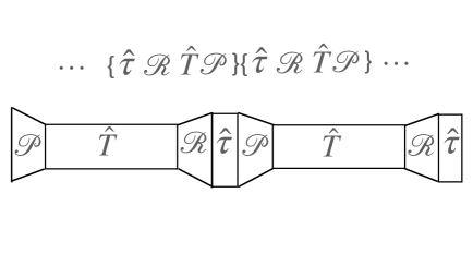
Figure 7: Schematics of the multiscale procedure described in the text. The idea is to run fine-grain quantum simulations for short stretches of time $\tau$ with the fine-grain propagator $\hat{\tau}$) so as to curb the effects of low success probabilities, and perform long stretches of sixe $t$ with coarse grained (classical) solvers ($\hat{T}$). Machine learning can help finding optimal versions of the projection and reconstruction operators minimizing the coarse-graining errors.

At this stage, it is impossible to predict whether telescopic quantum marchers, possibly equipped with machine-assisted multiscale coarse-graining, will ever hit the target of outdoing classical simulations. The topic is exciting and up for grabs.

V Summary

Summarizing, we have pointed out by means of a concrete example that the search for quantum algorithms for fluids bears a significant foundational value besides the potentially practical one. However, realizing the latter requires extremely efficient telescopic quantum time marchers far beyond the current state of the art. The topic is currently under active exploration.

- [1] W. Kohn, Nobel Lecture: Electronic structure of matter—wave functions and density functionals, Rev. Mod. Phys., 71, 1253, (1999)
- [2] D Poulin, A Qarry, R Somma, F Verstraete, Quantum simulation of time-dependent Hamiltonians and the convenient illusion of Hilbert space, Phys. Rev. Lett. 106 (17), 170501, (2011)
- [3] R. Feynman, Simulating Physics with Computers, Int. J. Mod Phys, 6, 467, (1982)
- [4] L. Kadanoff, Statistical Physics: Statics, Dynamics and Renormalization, World Scientific (2000)
- [5] O. Aharony, S.S. Gubser, J. Maldacena, H. Ooguri, Y. Oz, Large N Field Theories, String Theory and Gravity, Phys.Rept., 323:183-386, (2000)
- [6] R. Benzi, S. Succi, M. Vergassola, The lattice Boltzmann equation: theory and applications Physics Reports 222 (3), 145-197 (1992)
- [7] U. Frisch, B. Hasslacher, Y. Pomeau, Lattice-Gas Automata for the Navier-Stokes Equation, Physical Review Letters, 56, 1505 – Published 7 April, 1986
- [8] Becker, R. J. ”Lagrangian/Hamiltonian formalism for description of Navier-Stokes fluids.” Physical Review Letters 58.14 (1987): 1419.
- [9] J.P. Liu, H. O. Kolden, H. K. Krovi et al, Efficient quantum algorithm for dissipative nonlinear differential equations, PNAS, 118(35) e2026805118 (2021)
- [10] X. Li, X. Yin, N. Wiebe, J. Chun, GK Schenter, M. Cheung, J. Muelmenstadt, “Potential Quantum Advantage for Simulation of Fluid Dynamics.” Physical Review Research 7 (1) (2025) : 013036. https://doi.org/10.1103/PhysRevResearch.7.013036.
- [11] Lloyd, Seth, Giacomo De Palma, Can Gokler, Bobak Kiani, Zi-Wen Liu, Milad Marvian, Felix Tennie, and Tim Palmer. ”Quantum algorithm for nonlinear differential equations.” arXiv preprint arXiv:2011.06571 (2020).
- [12] Barenblatt, Grigory Isaakovich. Scaling, self-similarity, and intermediate asymptotics: dimensional analysis and intermediate asymptotics. No. 14. Cambridge University Press, 1996.
- [13] Ko Okumura , A renormalization group analysis of bubble breakup, Scientific Reports volume 15, Article number: 34507 (2025)
- [14] Jones, Billy D. ”Navier-Stokes Hamiltonian for the Similarity Renormalization Group.” arXiv preprint arXiv:1407.1035 (2014)
- [15] D. Deutsch, Quantum theory, the Church–Turing principle and the universal quantum computer, Proceedings of the Royal Society of London A. 400(1818):97-117, (1985)
- [16] M.A. Nielson, I.L. Chuang, Quantum Computation and Quantum Information: 10th Anniversary Edition, Cambridge University Press, 2010.
- [17] S. Succi, W. Itani, K. Sreenivasan and R. Steijl, Quantum computing for fluids, where do we stand? Europhysics Letters 144 (1), 10001, (2023)
- [18] T. Carleman, Acta Mathematica 59, 63 (1932).
- [19] Sanavio, C., R. Scatamacchia, C. de Falco, and S. Succi. 2024. “Three Carleman Routes to the Quantum Simulation of Classical Fluids.” Physics of Fluids 36 (5): 057143. https://doi.org/10.1063/5.0204955.
- [20] Sanavio, Claudio, and Sauro Succi. 2024. “Lattice Boltzmann–Carleman Quantum Algorithm and Circuit for Fluid Flows at Moderate Reynolds Number.” AVS Quantum Science 6 (2): 023802. https://doi.org/10.1116/5.0195549.
- [21] W. Itani and S. Succi, Analysis of Carleman linearization of lattice Boltzmann, Fluids, 7 (1) 24, (2022)
- [22] Sanavio, Claudio, William A. Simon, Alexis Ralli, Peter Love, and Sauro Succi, “Carleman-Lattice-Boltzmann Quantum Circuit with Matrix Access Oracles.” Physics of Fluids 37 (3): 037123 (2025). https://doi.org/10.1063/5.0254588.
- [23] D Caamps, L Lin, R Van Beeumen, C Yang, Explicit Quantum Circuits for Block Encodings of Certain Sparse Matrices, SIAM Journal on Matrix Analysis and Applications 45 (1), 801-827 (2024)
- [24] Gilyén, A., Y. Su, G. H. Low, and N. Wiebe, “Quantum Singular Value Transformation and beyond: Exponential Improvements for Quantum Matrix Arithmetics.” Proceedings of the 51st Annual ACM SIGACT Symposium on Theory of Computing (New York, NY, USA), STOC 2019, 193–204. https://doi.org/10.1145/3313276.3316366 (2019).
- [25] A. A. Zecchi, C. Sanavio, S. Perotto, and S. Succi, ”Telescopic quantum simulation of the advection-diffusion-reaction dynamics” arxiv:2509.
- [26] U. Frisch, Fluid turbulence, Cambridge Univ. Press, (1995)
- [27] https://github.com/ProjectPhysX/FluidX3D
- [28] F. Tennie and TN Palmer, Quantum computers for weather and climate prediction: the good the bad and the noisy, arXiv:2210.17460v1 [quant-ph] 31 Oct 2022
- [29] A. A. Zecchi, C. Sanavio, S. Perotto, and S. Succi, Improved Amplitude Amplification Strategies for the Quantum Simulation of Classical Transport Problems, Quantum Science and Technology 10 (2025) (3): 035039. https://doi.org/10.1088/2058-9565/addeea.
- [30] Dmitrii Kochkov, Jamie A. Smith, Ayya Alieva and Stephan Hoyer, Machine learning–accelerated computational fluid dynamics, PNAS, May 18, 118 (21) e2101784118, (2021)
- [31] Maida Wang,Xiao Xue,Mingyang Gaoand Peter V. Coveney, Quantum-informed machine learning for the prediction of chaotic dynamical systems, arXiv:2507.19861v3 [quant-ph] 28 Aug 2025