An exactly solvable asymmetric simple inclusion process

Abstract

We study a generalization of the asymmetric simple inclusion process (ASIP) on a periodic one-dimensional lattice, where the integers in the particles rates are deformed to their $t$-analogues. We call this the $(q,t,\theta)$ ASIP, where $q$ is the asymmetric hopping parameter and $\theta$ is the diffusion parameter. We show that this process is a misanthrope process, and consequently the steady state is independent of $q$. We compute the steady state, the one-point correlation and the current in the steady state. In particular, we show that the single-site occupation probabilities follow a beta-binomial distribution at $t=1$. We compute the two-dimensional phase diagram in various regimes of the parameters $(t,\theta)$ and perform simulations to justify the results. We also show that a modified form of the steady state weights at $t\neq 1$ satisfy curious palindromic and antipalindromic symmetries. Lastly, we define an enriched process at $t=1$ and $\theta$ an integer which projects onto the $(q,1,\theta)$ ASIP and whose steady state is uniform, which may be of independent interest.

1 Introduction

The asymmetric simple exclusion process (ASEP) in one-dimensions is an extremely well-studied interacting particle system both in statistical physics and in mathematics. It is important from the point of view of nonequilibrium statistical physics because it is exactly solvable and explicit calculations have led to a lot of insight into nonequilibrium phenomena in one dimension. It has also turned out to be of great interest in different areas of mathematics such as combinatorics, probability theory and representation theory. In the ASEP, every site has at most one particle and particles hop preferentially onto neighbouring sites provided they are empty. Therefore, one can think of it as a ‘fermionic’ process. And indeed, like in fermionic statistics, particles in the ASEP do tend to repel each other.

It is natural to consider a ‘bosonic’ counterpart of the ASEP, and a symmetric analog known as the symmetric inclusion process (SIP) was first introduced and studied in its own right by Giardinà–Redig–Vafayi [GRV10] from the point of view of obtaining correlation inequalities. We add that a model very similar in spirit is implicit in the works of Giardinà–Kurchan–Redig [GKR07, Section III] and Giardinà–Kurchan–Redig–Vafayi [GKRV09, Section 5.2], where they obtain it as the dual of a system with Brownian interactions. Unlike the ASEP, the inclusion process permits multiple particles per site and the dynamics promotes aggregation. Roughly speaking, if two neighbouring sites have $a$ and $b$ particles, the rate in the SIP at which a particle moves from the first to the second is $a(\theta+b)$ and from the second to the first is $b(\theta+a)$, where $\theta$ is a free parameter, called the diffusion parameter in the literature.

The asymmetric inclusion process (ASIP), first proposed by Grosskinsky–Redig–Vafayi [GRV11], is a natural variant of the SIP, where particles hop preferentially in one direction. They studied the ASIP in the one-dimensional lattice with closed boundaries, and it was extended to two variants of the ASIP with periodic boundary conditions by Cao–Chleboun–Grosskinsky [CCG14]. Both these works study condensation phenomena both in and out of equilibrium in certain limits of the rates. A lot of work has been done since then on condensation in the ASIP. We refer to the survey by Landim [Lan19] for more details. To be more precise, [CCG14] studied two variants of the ASIP. The first was precisely the SIP (with symmetric hopping rates), and the second was with totally asymmetric hopping rates, which they call the TASIP. We simultaneously generalize both the models in this work. Specifically, we generalize the form of the rates mentioned above to $[a]_{t}(\theta+[b]_{t})$, where $[n]_{t}$ is the $t$-analogue of the integer $n$, and we add an asymmetry parameter $q$; see Section 2 for the precise definition. We call this model the $(q,t,\theta)$ ASIP. In the limit $t\to 1$, we obtain both the variants studied in [CCG14] at $q=0$ and $q=1$. To clarify, we only focus on the steady state. We will show that many of the properties of the ASIP continue to hold for the $(q,t,\theta)$ ASIP.

After the definition of the $(q,t,\theta)$ ASIP in Section 2, we will show that this is a special case of a misanthrope process [CT85, EW14], and so the steady state will be of product form. In Section 3, we give explicit formulas for the steady states and derive some properties. It will turn out that the analysis for $t=1$ and $t\neq 1$ will be different, and these will be studied separately throughout. We look at observables in the steady state in Section 4. In particular, we will show that the one-point distribution is the so-called beta-binomial distribution (which generalizes the beta distribution) and calculate the current when $t=1$.

In Section 5, we derive the phase diagram of the $(q,t,\theta)$ ASIP in terms of the parameters $\theta$ and $t$. Although we are unable to give exact results, we explain the phases in various limiting regions of the diagram. We also attach movies as ancillary files together with this submission in these regions and include snapshots of these movies. In some cases, the simulation results do not seem to match calculations, and we explain why in each of these cases.

When $t\neq 1$, we use an alternate parameterization of the rates by replacing $\theta$ by another parameter $a$, and show that the steady state weights are either palindromic or antipalindromic polynomials jointly in the variables $a,t$ in Section 6. This is similar in spirit to a result we had obtained earlier for the $(q,t)$ $K$-ASEP [AM24] in a single parameter.

Lastly, in Section 7, we construct an enriched process when $t=1$ and $\theta$ is a positive integer which projects as a Markov process onto the $(q,t,\theta)$ ASIP. We show that the steady state of this enriched process is uniform, and thus obtain an alternate proof of the steady state formula when $t=1$.

2 Model description

We define an asymmetric simple inclusion process, denoted $(q,t,\theta)$ ASIP, on a periodic one-dimensional lattice characterized by the following parameters: the number of sites $L\in\mathbb{N}$ (sites $1$ and $L$ are adjacent) and the total number of particles $n\in\mathbb{N}$, the asymmetry parameter $q\geq 0$ which distinguishes the forward and backward transition rates, and diffusion parameter $\theta>0$ appearing in the target site contribution (to which the particle hops), and the deformation parameter $t\geq 0$. All particles are indistinguishable and can occupy any site. We denote the set of all configurations by

$$\Omega_{L,n}=\left\{\eta=(\eta_{1},\eta_{2},\ldots,\eta_{L})\in\{0,1,\dots,n\}^{L}\Biggm|\sum_{i=1}^{L}\eta_{i}=n\right\}.$$ (1)

The total number of configurations $\bigm|\Omega_{L,n}\bigm|$ is thus given by the number of ways of distributing $n$ particles among $L$ sites, or the number of compositions of $n$ into $L$ non-negative parts giving

$$\bigm|\Omega_{L,n}\bigm|=\binom{n+L-1}{n}.$$ (2)

To illustrate this, we can take a small example with $L=3$ sites and $n=4$ particles, giving us

$$\Omega_{3,4}=\begin{Bmatrix}(0,0,4),(0,1,3),(0,2,2),(0,3,1),(0,4,0),\\ (1,0,3),(1,1,2),(1,2,1),(1,3,0),(2,0,2),\\ (2,1,1),(2,2,0),(3,0,1),(3,1,0),(4,0,0)\end{Bmatrix}$$ (3)

and

$$\bigm|\Omega_{3,4}\bigm|=\binom{6}{4}=15.$$ (4)

To define the rates of the $(q,t,\theta)$ ASIP, we recall the $t$-analogue of a nonnegative integer $k$ as

$$[k]_{t}=\frac{1-t^{k}}{1-t}=\begin{cases}\displaystyle\sum_{i=0}^{k-1}t^{i}&\text{for }t\neq 1,\\ k&\text{for }t=1.\end{cases}$$ (5)

For later purposes, we define the $t$-factorial of a nonnegative integer as

$$[k]_{t}!=[k]_{t}[k-1]_{t}\cdots[1]_{t},$$ (6)

and the $t$-binomial coefficient or Gaussian polynomial as

$${\begin{bmatrix}m\\ n\end{bmatrix}_{\!t}}=\frac{[m]_{t}!}{[n]_{t}![m-n]_{t}!},$$ (7)

where $m$ and $n$ are nonnegative integers with $n\leq m$. The $(q,t,\theta)$ ASIP is a simple process, meaning that particles can only hop between neighbouring sites. We will denote configurations by $\eta=(\eta_{1},\eta_{2},\ldots,\eta_{L})\in\Omega_{L,n}$, where $\eta_{i}$ denotes the number of particles at site $i$, also known as the occupation number. The transitions are as follows. For two neighbouring sites indexed $(i,i+1)$ having occupation numbers $(\alpha,\beta)$ respectively,

$$(\alpha,\beta)\rightarrow(\alpha-1,\beta+1)\quad\text{with rate}\quad[\alpha]_{t}(\theta+[\beta]_{t})$$ (8)

for the forward transition, and

$$(\alpha,\beta)\rightarrow(\alpha+1,\beta-1)\quad\text{with rate}\quad q\,[\beta]_{t}(\theta+[\alpha]_{t})$$ (9)

for the reverse transition. A special case of our model, namely $t=1$, coincides with a special case of the model studied by Grosskinsky–Redig–Vafayi [GRV11, Section 3]. These rates are automatically $0$ when the source site is empty, so a transition out of an empty site is forbidden. See Figure 1 for an illustration.

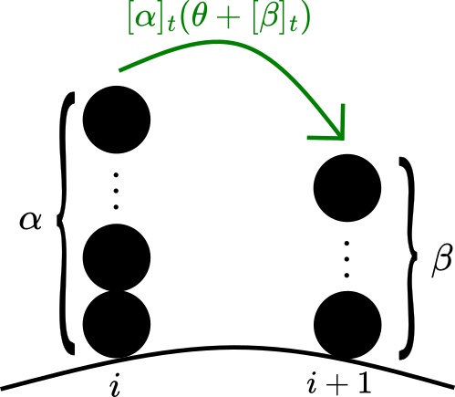
(a) Forward transition rate

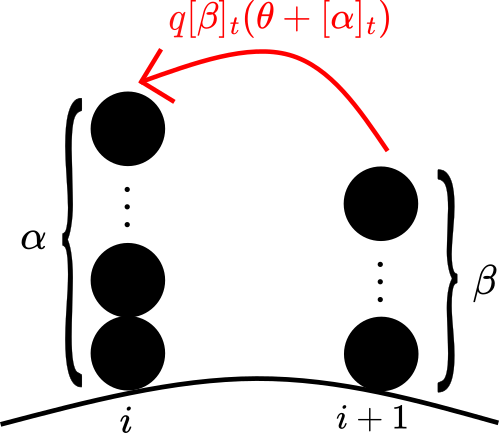
(b) Backward transition rate

Figure 1: Transition rates between two consecutive sites indexed by $i$ and $i+1$ in clockwise order having particles $\alpha$ and $\beta$ respectively.

To establish the relationship between the $(q,t,\theta)$ ASIP and the broader class of misanthrope processes, we verify the fundamental constraints. Recall that a misanthrope process is a simple process in which the transition rate for a neighbouring pair of sites containing $(\alpha,\beta)$ particles to transition to $(\alpha-1,\beta+1)$ is $u(\alpha,\beta)$. It has been shown [CT85, EW14] that when the rates satisfy the conditions

$$\frac{u(\beta,\alpha)}{u(\alpha+1,\beta-1)}=\frac{u(1,\alpha)u(\beta,0)}{u(\alpha+1,0)u(1,\beta-1)},$$ (10)

and

$$u(\beta,\alpha)-u(\alpha,\beta)=u(\beta,0)-u(\alpha,0)$$ (11)

we get a product form for the steady state which is independent of $q$. For the totally asymmetric ASIP (i.e. the $(0,t,\theta)$ ASIP), we have the rate

$$u(\alpha,\beta)=[\alpha]_{t}(\theta+[\beta]_{t}),$$ (12)

and the left-hand side of (10) is

$$\frac{u(\beta,\alpha)}{u(\alpha+1,\beta-1)}=\frac{[\beta]_{t}(\theta+[\alpha]_{t})}{[\alpha+1]_{t}(\theta+[\beta-1]_{t})},$$ (13)

which is equal to the right-hand side

$$\frac{u(1,\alpha)u(\beta,0)}{u(\alpha+1,0)u(1,\beta-1)}=\frac{(\theta+[\alpha]_{t})[\beta]_{t}\theta}{[\alpha+1]_{t}\theta(\theta+[\beta-1]_{t})}.$$ (14)

Similarly, the left-hand side of (11) is

$$u(\beta,\alpha)-u(\alpha,\beta)=[\beta]_{t}(\theta+[\alpha]_{t})-[\alpha]_{t}(\theta+[\beta]_{t})=\theta([\beta]_{t}-[\alpha]_{t}),$$ (15)

which is equal to the right-hand side

$$u(\beta,0)-u(\alpha,0)=[\beta]_{t}\theta-[\alpha]_{t}\theta=\theta([\beta]_{t}-[\alpha]_{t}).$$ (16)

This verification confirms that the $(0,t,\theta)$ ASIP belongs to the class of misanthrope processes, and thus the steady state is of product form. By standard arguments, it is also clear that the steady state of the $(q,t,\theta)$ ASIP is the same as that of the $(0,t,\theta)$ ASIP and hence, independent of $q$.

When $t\neq 1$, we also parametrize our rates differently in terms of

$$\theta=\frac{1-a}{a(1-t)},$$ (17)

so that the transitions depend on $a$ and $t$. In this notation,

$$(\alpha,\beta)\rightarrow(\alpha-1,\beta+1)\quad\text{with rate}\quad[\alpha]_{t}\left(\frac{1-a}{a(1-t)}+[\beta]_{t}\right)=\frac{[\alpha]_{t}(1-at^{\beta})}{a(1-t)},$$ (18)

and

$$(\alpha,\beta)\rightarrow(\alpha+1,\beta-1)\quad\text{with rate}\quad q\,[\beta]_{t}\left(\frac{1-a}{a(1-t)}+[\alpha]_{t}\right)=\frac{q[\beta]_{t}(1-at^{\alpha})}{a(1-t)}.$$ (19)

We will focus on this formulation only while discussing palindromic symmetry in Section 5.

3 Steady state

Having established that the $(q,t,\theta)$ ASIP belongs to the class of misanthrope processes, we now derive the exact form of the steady state. We begin with the general values of $t$ before specializing to $t=1$.

3.1 $t$ general

For $q\geq 0$ and $\theta>0$, it is easy to show that there is a sequence of transitions leading from any configuration in $\Omega_{L,n}$ to any other. This proves that the process is ergodic. Note that if $\theta=0$, no particle can enter an empty site, and ergodicity is broken. Hence, we require $\theta>0$. We focus on properties of the steady state, which is unique by ergodicity and which we denote by $\pi$. Thus, the probability of seeing any configuration $\eta=(\eta_{1},\eta_{2},\ldots,\eta_{L})\in\Omega_{L,n}$ in the long-time limit approaches $\pi(\eta)$. Using the result for the product state of a misanthrope process outlined in [EW14, Equation (22)],

$$f(m)=\prod_{i=1}^{m}\frac{u(1,i-1)}{u(i,0)},$$ (20)

and $\pi(\eta)\propto\prod_{i}f(\eta_{i})$. For the $(q,t,\theta)$ ASIP, this quantity is

$$f(m)=\prod_{i=1}^{m}\frac{\theta+[i-1]_{t}}{\theta[i]_{t}}.$$ (21)

Define the function $\varphi_{\theta,t}(m)$ by

$$\varphi_{\theta,t}(m)=\prod_{i=0}^{m-1}(\theta+[i]_{t}),$$ (22)

with $\varphi_{\theta,t}(0)=1$. We can rewrite (21) as

$$f(m)=\frac{\varphi_{\theta,t}(m)}{\theta^{m}[m]_{t}!},$$ (23)

We thus get the steady state weights using [EW14, Equation (4)] to be

$$\text{wt}_{\theta,t}(\eta)=\prod\limits_{i=1}^{L}f(\eta_{i})=\prod\limits_{i=1}^{L}\frac{\varphi_{\theta,t}(\eta_{i})}{\theta^{\eta_{i}}[\eta_{i}]_{t}!}.$$ (24)

By dropping the constant scaling factor of $\prod\limits_{i=1}^{L}\theta^{\eta_{i}}=\theta^{n}$ from the denominator and multiplying the numerator by a constant $[n]_{t}!$, we write the weights as

$$\text{wt}_{\theta,t}(\eta)={\begin{bmatrix}n\\ \eta_{1},\ldots,\eta_{L}\end{bmatrix}_{\!t}}\prod_{i=1}^{L}\varphi_{\theta,t}(\eta_{i})$$ (25)

where

$${\begin{bmatrix}n\\ \eta_{1},\ldots,\eta_{L}\end{bmatrix}_{\!t}}=\frac{[n]_{t}!}{[\eta_{1}]_{t}![\eta_{2}]_{t}!\ldots[\eta_{L}]_{t}!}$$ (26)

is the usual $t$-multinomial coefficient. As mentioned before, the steady state is of product form. Hence, weights of configurations depend only on the content and are independent of the ordering of sites. We can write its steady state probability as

$$\pi(\eta)=\frac{\text{wt}_{\theta,t}(\eta)}{Z_{L,n}}=\frac{1}{Z_{L,n}}{\begin{bmatrix}n\\ \eta_{1},\ldots,\eta_{L}\end{bmatrix}_{\!t}}\prod_{i=1}^{L}\varphi_{\theta,t}(\eta_{i})$$ (27)

where

$$Z_{L,n}=\sum_{\eta\in\Omega_{L,n}}\text{wt}_{\theta,t}(\eta)$$ (28)

is the nonequilibrium partition function which normalizes the probability distribution. The reader can verify that detailed balance holds at $q=1$, but not otherwise. The weight function defined in (25) is a bivariate polynomial of $\theta,t\in\mathbb{R^{+}}\setminus\{0\}$. As an example, the weights for the process with $L=3$ and $n=4$ are

$$\text{wt}_{\theta,t}(0,0,4) =\theta(\theta+1)(\theta+1+t)(\theta+1+t+t^{2}),$$ (29)

$$\text{wt}_{\theta,t}(0,1,3) =(1+t)(1+t^{2})\,\theta^{2}(\theta+1)(\theta+1+t),$$

$$\text{wt}_{\theta,t}(0,2,2) =(1+t^{2})(1+t+t^{2})\,\theta^{2}(\theta+1)^{2}$$

$$\text{wt}_{\theta,t}(1,1,2) =(1+t)(1+t^{2})(1+t+t^{2})\,\theta^{3}(\theta+1).$$

In the special case $\theta=1/t$, we obtain

$$\varphi_{1/t,t}(m)=\frac{1}{t}\left(\frac{1}{t}+[1]_{t}\right)\cdots\left(\frac{1}{t}+[m-1]_{t}\right)=\frac{[m]_{t}!}{t^{m}}$$ (30)

so the weight function (25) becomes

$$\textrm{wt}_{1/t,t}(\eta)=\frac{[n]_{t}!}{t^{n}}$$ (31)

which is the same for every configuration. Thus, the uniform distribution is the steady state in this case,

$$\pi(\eta)=\frac{1}{\bigm|\Omega_{L,n}\bigm|}=\frac{1}{\displaystyle\binom{L+n-1}{n}}.$$ (32)

3.2 $t=1$

We now turn our attention to the special case when $t=1$, where the model simplifies considerably. As mentioned above, this case at $q=0$ and $q=1$ has been studied in [CCG14], where they use the notation $d_{L}$ for what we call $\theta$. The transition rates discussed previously in (8) reduce to

$$(\alpha,\beta)\rightarrow(\alpha-1,\beta+1)\quad\textrm{with rate}\quad\alpha\,(\theta+\beta),$$ (33)

and the reverse transition (9) becomes

$$(\alpha,\beta)\rightarrow(\alpha+1,\beta-1)\quad\textrm{with rate}\quad q\,\beta\,(\theta+\alpha).$$ (34)

The $t$-multinomial coefficient also simplifies to the regular multinomial coefficient

$${\begin{bmatrix}n\\ \eta_{1},\eta_{2},\ldots,\eta_{L}\end{bmatrix}_{\!t=1}}=\binom{n}{\eta_{1},\eta_{2},\ldots,\eta_{L}}.$$

To express the weights in a more familiar form, we recall the rising factorial

$$x^{\overline{r}}=\frac{\Gamma(x+r)}{\Gamma(x)}=\frac{(x+r-1)!}{(x-1)!}=x\,(x+1)\dots(x+r-1),$$ (35)

for any real number $x$. We can thus simplify the steady state weight (25) to

$$\textrm{wt}_{\theta,1}=\binom{n}{\eta_{1},\dots,\eta_{L}}\prod_{i=1}^{L}\theta^{\overline{\eta_{i}}}$$ (36)

and the partition function is

$$Z_{L,n}=\sum_{\eta\in\Omega_{L,n}}\textrm{wt}_{\theta,1}$$ (37)

For example, when $L=3$ and $n=4$, substitute $t=1$ in (29) to obtain

$$Z_{3,4}=\sum_{\eta\in\Omega_{3,4}}\textrm{wt}_{\theta,1}(\eta)=81\theta^{4}+162\theta^{3}+99\theta^{2}+18\theta.$$ (38)

We now give a remarkable closed-form expression for the partition function when $t=1$. Recall the rising factorial variant of the Chu–Vandermonde identity [Com74, Equation [13d]], which states that

$$\sum^{n}_{i=0}\binom{n}{i}x^{\overline{i}}y^{\overline{n-i}}=(x+y)^{\overline{n}}.$$ (39)

Similarly, we have the analogous multinomial variant,

$$\sum_{\eta_{1}+\eta_{2}+\ldots+\eta_{L}=n}\binom{n}{\eta_{1},\eta_{2},\ldots,\eta_{L}}x_{1}^{\overline{\eta_{1}}}x_{2}^{\overline{\eta_{2}}}\ldots x_{L}^{\overline{\eta_{L}}}=(x_{1}+\ldots+x_{L})^{\overline{n}}.$$ (40)

Comparing this with our partition function for the weight function (36), we obtain

$$Z_{L,n}=\sum_{\eta_{1}+\cdots+\eta_{L}=n}\binom{n}{\eta_{1},\dots,\eta_{L}}\prod_{i=1}^{L}\theta^{\overline{\eta_{i}}}=(L\theta)^{\overline{n}}=L\theta(L\theta+1)\ldots(L\theta+n-1).$$ (41)

For our previous example, we obtain

$$Z_{3,4}=(3\theta)^{\overline{4}}=3\theta(3\theta+1)(3\theta+2)(3\theta+3)=81\theta^{4}+162\theta^{3}+99\theta^{2}+18\theta,$$

which matches the formula in (38).

4 Observables

We now calculate observables in the steady state of this process.

4.1 One-point correlation

Since multiple particles can occupy a single site, we can compute the distribution of the number of particles at a given site. We denote the steady state probability that there are $\alpha$ particles at site $i$ by $\langle\eta_{i}=\alpha\rangle$.

Since the steady state weights in (25) are of product form, we can easily show that

$$\langle\eta_{i}=\alpha\rangle={\begin{bmatrix}n\\ \alpha\end{bmatrix}_{\!t}}\varphi_{\theta,t}(\alpha)\frac{Z_{L-1,n-\alpha}}{Z_{L,n}},$$ (42)

for any site $i$. This is not easy to compute for general $\theta$ and $t$. But for $t=1$, the formulas become much simpler. Using (41), we get

$$\langle\eta_{i}=\alpha\rangle=\binom{n}{\alpha}\theta^{\overline{\alpha}}\frac{((L-1)\theta)^{\overline{n-\alpha}}}{(L\theta)^{\overline{n}}}.$$ (43)

This formula is also given in [CCG14, Page 526].

It turns out that there exists a distribution in the literature with the same probability mass function. This is called the beta-binomial distribution, denoted $\textrm{BetaBin}(n,\alpha,\beta)$, which depends on the size $n$, and two positive real parameters $\alpha$ and $\beta$. A random variable having this distribution counts the number of successes in $n$ Bernoulli trials, where the success probability is not fixed but is drawn from the well-known beta distribution [JKK05, Section 6.2.2]. Recall that the beta distribution $B(\alpha,\beta)$ is a continuous distribution on $[0,1]$ with probability density proportional to $x^{\alpha-1}(1-x)^{\beta-1}$. The normalizing constant is the beta function

$$B(x,y)=\frac{\Gamma(x)\Gamma(y)}{\Gamma(x+y)},$$

where $\Gamma$ is the gamma function

$$\Gamma(x)=\int\limits_{0}^{\infty}z^{x-1}e^{-z}dz.$$

The probability that a $\textrm{BetaBin}(n,\alpha,\beta)$ random variable $X$ takes value $x$ is given explicitly by

$$\mathbb{P}(X=x)=\binom{n}{x}\frac{B(x+\alpha,n-x+\beta)}{B(\alpha,\beta)}.$$ (44)

When $\alpha$ and $\beta$ are positive integers, the beta-binomial distribution becomes the negative hypergeometric distribution.

Starting from (43) and writing $\theta^{\overline{\alpha}}=\Gamma(\theta+\alpha)/\Gamma(\theta)$, a short calculation shows that

$$\langle\eta_{i}=\alpha\rangle=\binom{n}{\alpha}\frac{B(\alpha+\theta,n-\alpha+(L-1)\theta)}{B(\theta,(L-1)\theta)}.$$ (45)

Therefore, the distribution of particles at any site is given by the beta-binomial distribution $\textrm{BetaBin}(n,\alpha=\theta,\beta=(L-1)\theta)$.

From standard facts about the beta-binomial distribution [JKK05, Equation (6.12)], the average number of particles per site is

$$n\frac{\alpha}{\alpha+\beta}=\frac{n}{L},$$

which is evident from the translation-invariance of the $(q,t,\theta)$ ASIP, and the variance of the number of particles per site is

$$\frac{n\alpha\beta(\alpha+\beta+n)}{(\alpha+\beta)^{2}(\alpha+\beta+1)}=\frac{n(L-1)(L\theta+n)}{L^{2}(L\theta+1)}$$ (46)

Let $\rho\in[0,1]$ be a fixed constant. If we let $L,n\to\infty$ such that $n/L\to\rho$, then the variance approaches $\rho(\theta+\rho)$. See Table 1 for a comparison between the theoretical value of the variance and numbers from a numerical simulation for the $(q,1,\theta)$ ASIP with 6 sites and 15 particles.

$\theta$	Theoretical value	Simulation result	Error
$1/10=0.1$	20.3125	20.4164	0.50 %
$1/7=0.143$	17.78846	17.8761	0.48 %
$1/4=0.25$	13.75	14.0828	2.40 %
1	6.25	6.2558	0.09 %
3	3.61842	3.5551	1.75 %
6	2.87162	2.8769	0.18 %
10	2.56147	2.5776	0.39 %

Table 1: Comparision of the variance of the occupation number at the first site the $(0,1,\theta)$ ASIP with $L=6$ and $n=15$. The simulation results are averaged over 10000 steady states for 20 different runs.

4.2 Current at $t=1$

Just as for the one-point correlation, we do not have a closed-form formula for the current for general values of $t$ due to the lack of a closed-form expression for the partition function. So we will only calculate the current at $t=1$. This has been computed in the grand canonical ensemble in [CCG14, Page 526].

We derive the current by analyzing the net particle flow between neighbouring sites. Let us consider two consecutive sites labelled $i$ and $i+1$ having $\alpha$ and $\beta$ particles respectively. From the rates described in (33) and (34), we can write down the net rate of flow of particles between the two sites as

$$\alpha(\theta+\beta)-q\beta(\theta+\alpha)=(1-q)\alpha\beta+(\alpha-q\beta)\theta.$$

The steady state current $J$ is obtained by averaging this net flow over the steady state between these two sites where

$$J=\sum_{\alpha=0}^{n}\sum_{\beta=0}^{n-\alpha}\big((1-q)\alpha\beta+(\alpha-q\beta)\theta\big)\langle\eta_{i}=\alpha,\eta_{i+1}=\beta\rangle.$$ (47)

The two-point correlations also follow from the product form of the steady state weights as we showed for one-point correlations in (43), and we obtain

$$\langle\eta_{i}=\alpha,\eta_{i+1}=\beta\rangle=\binom{n}{\alpha}\binom{n-\alpha}{\beta}\theta^{\overline{\alpha}}\theta^{\overline{\beta}}\frac{((L-2)\theta)^{\overline{n-\alpha-\beta}}}{(L\theta)^{\overline{n}}}.$$ (48)

We compute the current by evaluating each term in the sum separately. The second term in the summation formula for $J$ in (47) is

$$\theta\sum_{\alpha=0}^{n}\sum_{\beta=0}^{n-\alpha}(\alpha-q\beta)\langle\eta_{i}=\alpha,\eta_{i+1}=\beta\rangle=\theta\sum_{\alpha=0}^{n}\sum_{\beta=0}^{n}(\alpha-q\beta)\langle\eta_{i}=\alpha,\eta_{i+1}=\beta\rangle,$$ (49)

where we have used the fact that $\langle\eta_{i}=\alpha,\eta_{i+1}=\beta\rangle=0$ whenever $\alpha+\beta>n$. Expanding this further, we get

$$\theta\sum_{\alpha=0}^{n}\alpha\Bigl(\sum_{\beta=0}^{n}\langle\eta_{i}=\alpha,\eta_{i+1}=\beta\rangle\Bigr)-q\theta\sum_{\beta=0}^{n}\beta\Bigl(\sum_{\alpha=0}^{n}\langle\eta_{i}=\alpha,\eta_{i+1}=\beta\rangle\Bigr)\\ =\theta\sum_{\alpha=0}^{n}\alpha\langle\eta_{i}=\alpha\rangle-q\theta\sum_{\beta=0}^{n}\beta\langle\eta_{i+1}=\beta\rangle,$$ (50)

which is just the difference of two one-point correlations. Thus

$$\theta\sum_{\alpha=0}^{n}\sum_{\beta=0}^{n-\alpha}(\alpha-q\beta)\langle\eta_{i}=\alpha,\eta_{i+1}=\beta\rangle=\frac{n\theta}{L}-q\frac{n\theta}{L}=\frac{(1-q)n\theta}{L}.$$ (51)

The evaluation of the first term for $J$ in (47) is slightly more complicated. We need to determine

$$\sum_{\alpha=0}^{n}\sum_{\beta=0}^{n-\alpha}\alpha\beta\,\langle\eta_{i}=\alpha,\eta_{i+1}=\beta\rangle.$$

Using (25), the two-point correlations can be easily derived, and this can be written as

$$\sum_{\alpha=0}^{n}\sum_{\beta=0}^{n-\alpha}\alpha\beta\binom{n}{\alpha}\binom{n-\alpha}{\beta}\frac{\theta^{\overline{\alpha}}\theta^{\overline{\beta}}((L-2)\theta)^{\overline{n-\alpha-\beta}}}{(L\theta)^{\overline{n}}}.$$ (52)

Letting $\kappa=(L-2)\theta$, the right hand side above becomes

$$\frac{n!}{(L\theta)^{\overline{n}}}\sum_{\alpha=1}^{n-1}\sum_{\beta=1}^{n-\alpha}\frac{\theta^{\overline{\alpha}}}{(\alpha-1)!}\frac{\theta^{\overline{\beta}}}{(\beta-1)!}\frac{\kappa^{\overline{n-\alpha-\beta}}}{(n-\alpha-\beta)!}.$$

It is easy to see that the rising factorial in (35) satisfies the identity $x^{\overline{n}}=x(x+1)^{\overline{n-1}}$. Using this, we can write the above sum as

$$\frac{n(n-1)\theta^{2}}{(L\theta)^{\overline{n}}}\sum_{\alpha=1}^{n-1}\sum_{\beta=1}^{n-\alpha}\binom{n-2}{\alpha-1,\beta-1,n-\alpha-\beta}(\theta+1)^{\overline{\alpha-1}}(\theta+1)^{\overline{\beta-1}}\kappa^{\overline{n-\alpha-\beta}}.$$

After using the multinomial Chu-Vandermonde identity in (40), it becomes

$$n(n-1)\theta^{2}\frac{(2\theta+\kappa+2)^{\overline{n-2}}}{(L\theta)^{\overline{n}}}.$$

Substituting back $\kappa=(L-2)\theta$ and simplifying, we obtain

$$\frac{n(n-1)\theta}{(L\theta+1)L}.$$ (53)

Adding the contributions from (51) and $(1-q)$ times the expression in (53) yields the exact expression for the steady state current,

$$J=\frac{(1-q)\,\theta\,n(L\theta+n)}{L(L\theta+1)}.$$ (54)

If we let $L,n\to\infty$ such that $n/L\to\rho$, then the current becomes $J=(1-q)\rho(\theta+\rho)$, which is also derived in [CCG14, Equation (24)], and which is $(1-q)$ times the limiting variance.

5 Phase diagram

We analyze the two-dimensional phase diagram of the $(q,t,\theta)$ ASIP in terms of the parameters $t$ and $\theta$ in the limit where both $L$ and $n$ go to infinity. Although there are no phase transitions, we show that there are crossovers and the steady state looks very different in different regions of the phase diagram.

We understand the most probable configurations by examining the polynomial structure of the steady state weights (25) and identifying the dominant terms in various asymptotic limits. We first establish key properties of the polynomial weights. Define the degree (resp. order) of a polynomial $p$ to be the largest (resp. smallest) exponent for variable $x$ with nonzero coefficient, denoted $\operatorname{deg}_{x}(p)$ (resp. $\operatorname{ord}_{x}(p)$). One can easily show

$$\operatorname{ord}_{t}(\text{wt}_{\theta,t}(\eta))=0,$$ (55)

and

$$\operatorname{deg}_{\theta}(\text{wt}_{\theta,t}(\eta))=n.$$ (56)

We now prove

$$\operatorname{ord}_{\theta}(\text{wt}_{\theta,t}(\eta))=L-n_{0}(\eta),$$ (57)

and

$$\operatorname{deg}_{t}(\text{wt}_{\theta,t}(\eta))=\frac{n(n-3)}{2}+L-n_{0}(\eta),$$ (58)

where $n_{0}(\eta)$ is the number of empty sites in the configuration $\eta$. From (22), we see that

$$\operatorname{ord}_{\theta}(\varphi_{\theta,t}(m))=\begin{cases}0&m=0,\\ 1&\textrm{otherwise},\end{cases}$$

and, since the $t$-multinomial coefficient has no dependence on $\theta$,

$$\operatorname{ord}_{\theta}(\text{wt}_{\theta,t}(\eta))=\operatorname{ord}_{\theta}\left(\prod\limits_{i=1}^{L}\varphi_{\theta,t}(\eta_{i})\right)=L-n_{0}(\eta).$$ (59)

Using $\operatorname{deg}_{t}([n]_{t}!)=n(n-1)/2$ we get

$$\operatorname{deg}_{t}\left({\begin{bmatrix}n\\ \eta_{1},\ldots,\eta_{L}\end{bmatrix}_{\!t}}\right)=\operatorname{deg}_{t}([n]_{t}!)-\sum_{i=1}^{L}\operatorname{deg}_{t}([\eta_{i}]_{t}!)=\frac{n^{2}}{2}-\sum\limits_{i=1}^{L}\frac{\eta_{i}^{2}}{2}.$$ (60)

Now for the remaining factor of $\prod\limits_{i=1}^{L}\varphi_{\theta,t}(\eta_{i})$, since

$$\operatorname{deg}_{t}(\theta+[j]_{t})=\begin{cases}0&\textrm{when }j=0,\\ j-1&\textrm{otherwise},\end{cases}$$

we get

$$\operatorname{deg}_{t}(\varphi_{\theta,t}(m))=\begin{cases}0&\textrm{when }m=0,\\ \frac{(m-1)(m-2)}{2}&\textrm{otherwise},\end{cases}$$

and therefore

$$\operatorname{deg}_{t}\left(\prod\limits_{i=1}^{L}\varphi_{\theta,t}(\eta_{i})\right)=\sum\limits_{\begin{subarray}{c}i=1\\ \eta_{i}\neq 0\end{subarray}}^{L}\Bigl(\frac{\eta_{i}^{2}}{2}-\frac{3\eta_{i}}{2}+1\Bigr)=\sum\limits_{i=1}^{L}\frac{\eta_{i}^{2}}{2}-\frac{3n}{2}+L-n_{0}(\eta).$$ (61)

Therefore, using (25) and adding the results from (60) and (61), we get (58). The reader can verify (55)-(58) for the $(q,t,\theta)$ ASIP with $L=3$ and $n=4$ by looking at (29).

We now analyse the phase diagram in various regions. To do so we will now estimate $\varphi_{\theta,t}(\eta)$ and ${\begin{bmatrix}n\\ \eta_{1},\ldots,\eta_{L}\end{bmatrix}_{\!t}}$ in different ranges of t. We start by taking extreme limits for $t$ and see what simplifications can be made when it is either very small or very large. When $t\ll 1$ we can write

$$[m]_{t}=\sum_{i=0}^{m-1}t^{i}\begin{cases}=0\qquad&\textrm{when }\eta_{i}=0,\\ \approx 1\qquad&\textrm{otherwise }.\end{cases}$$

This simplifies the $t$-multinomial coefficient to

$${\begin{bmatrix}n\\ \eta_{1},\eta_{2},\ldots,\eta_{L}\end{bmatrix}_{\!t}}\approx 1,$$ (62)

and $\varphi_{\theta,t}(\eta_{i})$ to

$$\varphi_{\theta,t}(\eta_{i})=(\theta)(\theta+[1]_{t})\ldots(\theta+[\eta_{i}-1]_{t})\begin{cases}=1\qquad&\textrm{when }\eta_{i}=0,\\ \approx\theta(\theta+1)^{\eta_{i}-1}\qquad&\textrm{otherwise}.\end{cases}$$ (63)

On the other hand, when $t\gg 1$, the only simplification we have is

$$[m]_{t}=\sum_{i=1}^{m-1}t^{m}\begin{cases}=1\qquad&\textrm{when }m=0,\\ \approx t^{m-1}\qquad&\textrm{otherwise, }\end{cases}$$ (64)

In the following subsections, we will analyze the cases when $t\ll 1$, $t=1$ and $t\gg 1$ in that order. Finally, we will consider the special case $\theta t=1$.

5.1 $t\ll 1$ and $\theta\ll 1$

In this regime, we see strong particle aggregation phenomena. The condition $\theta\ll 1$ in (63) simplifies it to

$$\varphi_{\theta,t}(\eta_{i})\begin{cases}=1\qquad&\textrm{when }\eta_{i}=0,\\ \approx\theta\qquad&\textrm{otherwise},\end{cases}$$ (65)

and using (62) along with it we get

$$\text{wt}_{\theta,t}(\eta)\approx\theta^{L-n_{0}(\eta)}.$$ (66)

Since $\theta\ll 1$, the configurations with the highest probability will be the ones which minimize $L-n_{0}(\eta)$ i.e. maximizing $n_{0}(\eta)$. In any given configuration $\eta$ the maximum number of empty sites possible are

$$\textrm{max}(n_{0}(\eta))=L-1,$$ (67)

which happens when all the particles occupy the same site. Thus, we see grouping of particles in a single site, showing the phenomenon of strong condensation, first coined in [EW14]. Calculations for the example in (29) with the parameter values $\theta=t=0.0001$ gives the steady state probabilities

$$\pi(0,0,4)=0.33,\pi(0,1,3)=3.32\times 10^{-5},\pi(0,2,2)=3.33\times 10^{-5},\pi(1,1,2)=3.33\times 10^{-9}.$$

See the movie t_.0001_theta_.0001.mp4 among the ancillary files for a simulation of the $(0,0.0001,0.0001)$ ASIP with $L=n=20$. A snapshot from that movie is shown in Figure 2.

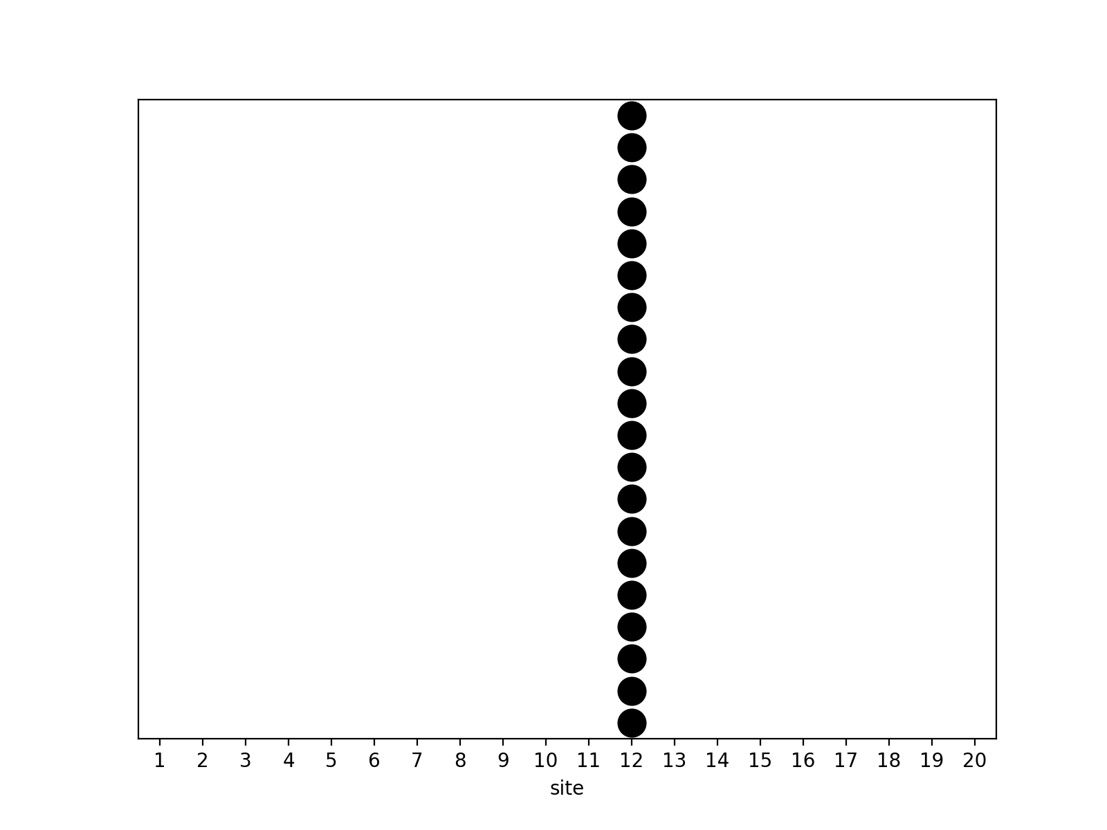
Figure 2: A snapshot of the $(0,0.0001,0.0001)$ ASIP with $L=20$ and $n=20$ in steady state.

5.2 $t\ll 1$ and $\theta\gg 1$

In this regime, we see an approximate uniform distribution across configurations. Using (62) and adding the condition $\theta\gg 1$ in (63), we obtain

$$\varphi_{\theta,t}(\eta_{i})\begin{cases}=1\qquad&\textrm{when }\eta_{i}=0,\\ \approx\theta^{\eta_{i}}\qquad&\textrm{otherwise}.\end{cases}$$ (68)

Therefore for any state $\eta$ we will have

$$\text{wt}_{\theta,t}(\eta)\approx\prod\limits_{i=1}^{L}\theta(\theta+1)^{\eta_{i}-1}\approx\theta^{n},$$ (69)

which is roughly the same for all configurations, so

$$\pi(\eta)\approx\frac{1}{\displaystyle\binom{L+n-1}{n}}.$$ (70)

Consider states where the particles are as evenly spread out as possible. We call these flattened states. Such states will have a higher probability as compared to others due to the higher value of its multinomial coefficient. One might expect to see flattened states in simulations because they have the highest probability. However, that is not the case and the reason is as follows. Due to the approximate uniform nature of the distribution, states with a larger number of permutations show up a lot more in simulations. The number of flattened states is a lot less than the number of states that have different number of particles in different sites. So we are more likely to see configurations with different number of particles in different sites and this will cause particles to cluster together. We call this phenomenon weak condensation.

Calculations for the example in (29) with the parameter values $\theta=1000$ and $t=0.01$ give the steady state probabilities

$$\pi(0,0,4)\approx 6.60\times 10^{-2},\pi(0,1,3)\approx 6.66\times 10^{-2},\\ \pi(0,2,2)\approx 6.66\times 10^{-2},\pi(1,1,2)\approx 6.72\times 10^{-2}.$$

See the movie t_.0001_theta_500.mp4 among the ancillary files for a simulation of the $(0,0.0001,500)$ ASIP with $L=n=20$. A snapshot from that movie is shown in Figure 3.

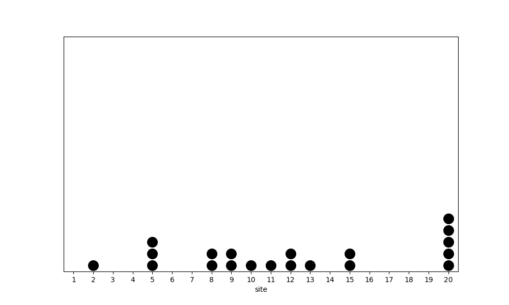
Figure 3: A snapshot of the $(0,0.0001,500)$ ASIP with $L=20$ and $n=20$ in steady state.

5.3 $t=1$ and $\theta\ll 1$

We find that this regime leads to condensation behaviour. Some nice simplifications have already been done for the $t=1$ case in (36) and further adding $\theta\ll 1$ we get

$$\textrm{wt}_{\theta,1}(\eta)\approx\binom{n}{\eta_{1},\dots,\eta_{L}}\prod\limits_{\begin{subarray}{c}i=1\\ \eta_{i}\neq 0\end{subarray}}^{L}\theta(1)(2)\ldots(\eta_{i}-1)=\binom{n}{\eta_{1},\dots,\eta_{L}}\prod\limits_{\begin{subarray}{c}i=1\\ \eta_{i}\neq 0\end{subarray}}^{L}\theta(\eta_{i}-1)!$$ (71)

giving

$$\textrm{wt}_{\theta,1}(\eta)\approx\binom{n}{\eta_{1},\dots,\eta_{L}}\theta^{L-n_{0}(\eta)}\prod\limits_{\begin{subarray}{c}i=1\\ \eta_{i}\neq 0\end{subarray}}^{L}(\eta_{i}-1)!=\frac{n!\;\theta^{L-n_{0}(\eta)}}{\prod\limits_{\begin{subarray}{c}i=1\\ \eta_{i}\neq 0\end{subarray}}^{L}\eta_{i}},$$ (72)

where the dominating factor is $\theta^{L-n_{0}(\eta)}$ which comes from every non-empty site and the factor in the denominator is subdominant. Since $\theta\ll 1$, $L-n_{0}(\eta)$ must be minimized. As discussed earlier, this happens when the maximum value of $n_{0}(\eta)$ is achieved as shown before in (67). Thus, condensate states are the most likely configurations. Numerical verification demonstrates this condensation phenomenon for example (29) with parameters $\theta=0.002$ and $t=1$ we get the steady state probability distribution

$$\pi(0,0,4)\approx 0.33,\pi(0,1,3)\approx 8.81\times 10^{-4},\pi(0,2,2)\approx 6.62\times 10^{-4},\pi(1,1,2)\approx 2.64\times 10^{-6}.$$

See the movie t_1_theta_.0001.mp4 among the ancillary files for a simulation of the $(0,1,\allowbreak 0.0001)$ ASIP with $L=n=20$. A snapshot from that movie is shown in Figure 4.

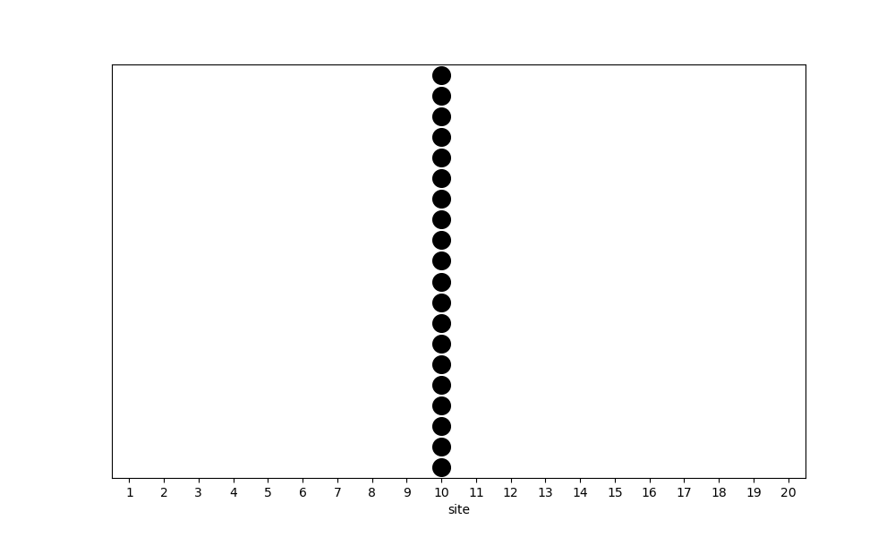
Figure 4: A snapshot of the $(0,1,0.0001)$ ASIP with $L=20$ and $n=20$ in steady state.

5.4 $t=1$ and $1\ll n\ll\theta$

For large $\theta$ when $t=1$, after adding an additional condition of $n\ll\theta$, we can write (36) as

$$\textrm{wt}_{\theta,1}\approx\binom{n}{\eta_{1},\dots,\eta_{L}}\prod\limits_{\begin{subarray}{c}i=1\\ \eta_{i}\neq 0\end{subarray}}^{L}\theta(\theta+1)\ldots(\theta+\eta_{i}-1)=\binom{n}{\eta_{1},\dots,\eta_{L}}\theta^{n}.$$ (73)

Dropping the common factor $\theta^{n}$ from all the weights, we get

$$\textrm{wt}_{\theta,1}\approx\binom{n}{\eta_{1},\dots,\eta_{L}},$$ (74)

which is again maximum for flattened states. For the example in (29) with parameters $\theta=10000$ and $t=1$, we get the steady state probability distribution

$$\pi(0,0,4)\approx 1.24\times 10^{-2},\pi(0,1,3)\approx\pi(3,1,0)=4.94\times 10^{-2},\\ \pi(0,2,2)\approx 7.41\times 10^{-2},\pi(1,1,2)\approx 0.148.$$

Following the argument in Section 5.2, we again see weak condensation in simulations as opposed to flattened states. To illustrate this, consider a system with $L=3$ and $n=6$, and parameters $\theta=2000$ and $t=1$. Here the flattened state has probability $\pi(2,2,2)=0.123$, which is clearly larger than $\pi(1,2,3)=0.082$. However, there is only one flattened state $(2,2,2)$. On the other hand, there are $6$ states with occupation numbers $1,2$ and $3$. So in the simulation, the probability of seeing the flattened state is $0.123$, whereas the probability of seeing a state with occupation numbers $1,2,3$ is $0.492$ which is much larger. See the movie t_1_theta_2000.mp4 among the ancillary files for a simulation of the $(0,1,2000)$ ASIP with $L=n=20$. A snapshot from that movie is shown in Figure 5.

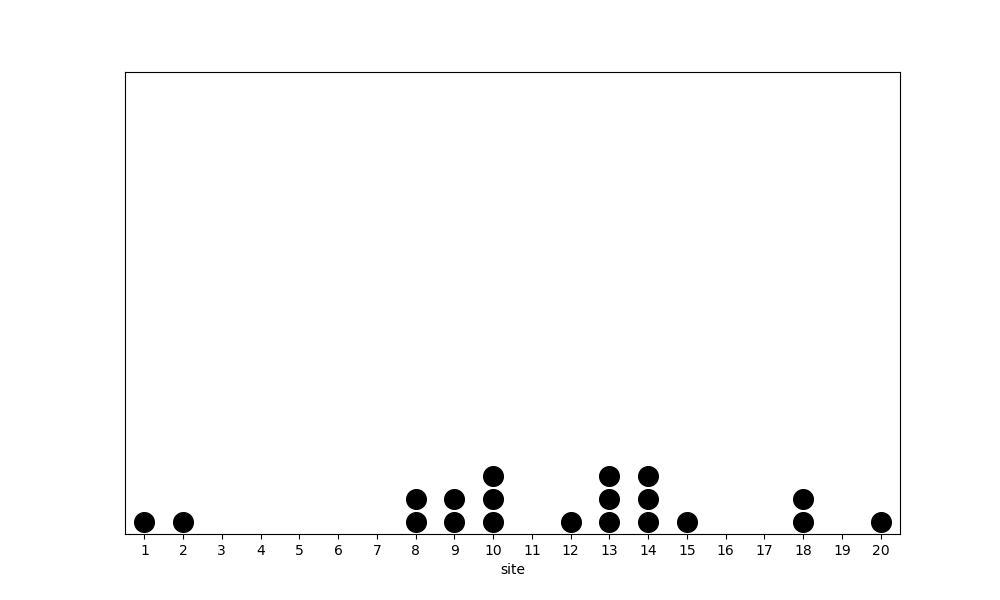
Figure 5: A snapshot of the $(0,1,2000)$ ASIP with $L=20$ and $n=20$ in steady state.

5.5 $\theta\ll 1\ll t$ and $\theta t\ll 1$

This region again favours stronger condensation similar to Section 5.1. Using (64) along with $\theta\ll 1$ will simplify (22) as

$$\varphi_{\theta,t}(\eta_{i})\begin{cases}=1\qquad&\textrm{when }\eta_{i}=0,\\ \approx\theta t^{\frac{(\eta_{i}-1)(\eta_{i}-2)}{2}}\qquad&\textrm{otherwise}.\end{cases}$$ (75)

Combining this with the largest term from the multinomial coefficient we can write

$$\text{wt}_{\theta,t}(\eta)=\theta^{L-n_{0}(\eta)}t^{\operatorname{deg}_{t}(\text{wt}_{\theta,t}(\eta))}+\textrm{ other terms }$$

where $n_{0}(\eta)$ is the number of empty sites in the configuration $\eta$. Using the formula for $\operatorname{deg}_{t}(\text{wt}_{\theta,t}(\eta))$ given in (58) we obtain

$$\text{wt}_{\theta,t}(\eta)\approx\theta^{L-n_{0}(\eta)}t^{\frac{n(n-3)}{2}+L-n_{0}(\eta)}=(\theta t)^{L-n_{0}(\eta)}t^{\frac{n(n-3)}{2}}.$$ (76)

The configuration with the highest steady state probability will therefore be dictated by the value of $\theta t$ which we will now explore. To maximize the weight (76) when $\theta t\ll 1$, we want to minimize $L-n_{0}(\eta)$, and hence maximize $n_{0}(\eta)$. So the dominant steady state becomes the condensate states where the value $n_{0}(\eta)$ takes its maximum value $L-1$ as in (67). Calculations for the example in (29) with the parameter values $\theta=0.000002$ and $t=1000$ give the steady state probabilities

$$\pi(0,0,4)\approx 0.33,\pi(0,1,3)\approx 6.62\times 10^{-4},\pi(0,2,2)\approx 6.62\times 10^{-4},\pi(1,1,2)\approx 1.33\times 10^{-6}.$$

See the movie t_500_theta_.0001.mp4 among the ancillary files for a simulation of the $(0,500,0.0001)$ ASIP with $L=n=20$. A snapshot from that movie is shown in Figure 6.

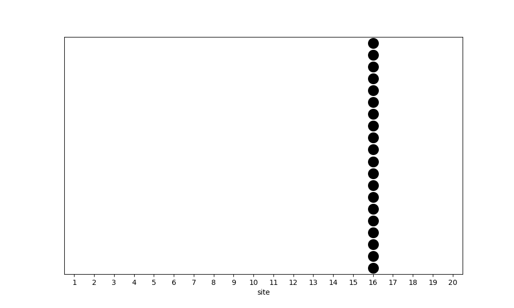
Figure 6: A snapshot of the $(0,500,0.0001)$ ASIP with $L=20$ and $n=20$ in steady state.

5.6 $\theta\ll 1\ll t$ and $\theta t\gg 1$

For $\theta\ll 1\ll t$ we analyze (76), this time for $\theta t\gg 1$. Here $L-n_{0}(\eta)$ must be maximized. For any state $\eta$ we have

$$\min(n_{0}(\eta))=\begin{cases}L-n&\textrm{when }n<L,\\ 0&\textrm{otherwise}.\end{cases}$$

Therefore, when $n\leq L$, there will at most be one particle per site in the likely configurations. When $L\leq n$, all sites are occupied. This time, flattened states will dominate because the $t$-multinomial coefficient is larger for such states. Numerical calculations confirm the preference for flattened configurations. For example,in (29) with parameters $\theta=0.002$ and $t=10^{6}$, we get the steady state probability distribution

$$\pi(0,0,4)\approx 8.32\times 10^{-8},\pi(0,1,3)\approx 1.66\times 10^{-4},\pi(0,2,2)\approx 1.66\times 10^{-4},\pi(1,1,2)\approx 0.33.$$

See the movie t_10000_theta_.01.mp4 among the ancillary files for a simulation of the $(0,10000,0.01)$ ASIP with $L=n=20$. A snapshot from that movie is shown in Figure 7.

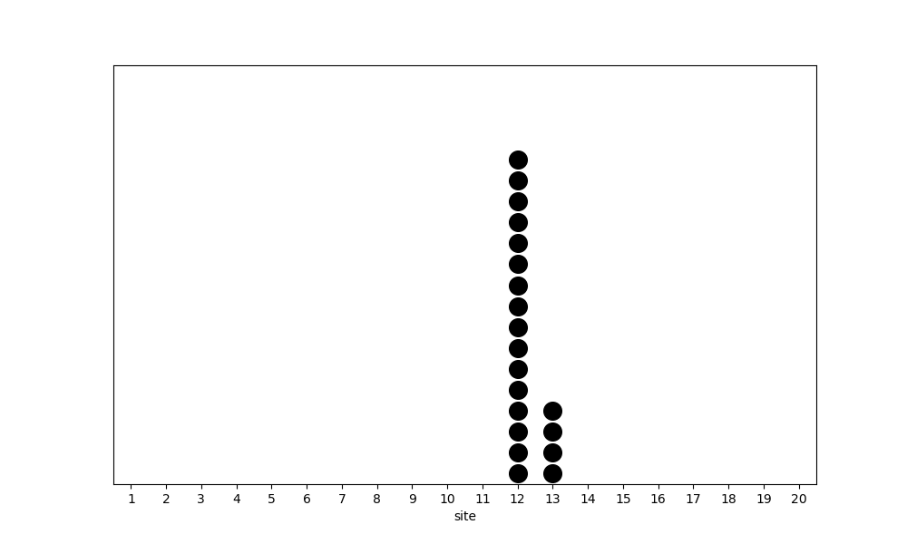
Figure 7: A snapshot of the $(0,10000,0.01)$ ASIP with $L=20$ and $n=20$ in steady state.

Remark 5.1.

When $t\gg 1$, the most dominant term of $t$ in the forward rates defined in (8) is $t^{\alpha+\beta-2}$. This rate spans many decades for most configurations even in a moderately sized system. We use the Gillespie algorithm [Gil76], which keeps track of successive states and their holding times. For such vastly varying transition rates, we have the problem of registering all these astronomical numbers of fast transitions and their extremely small holding times. Therefore, states with more particles in neighboring sites tend to dominate (since both $\alpha$ and $\beta$ are large) in simulations, and we are unable to see states with fewer particles in sites. This is why the movie and the snapshot do not match the analysis whenever $t\gg 1$.

5.7 $1\ll\theta\ll t$

Using (64) and simplifying

$$\varphi_{\theta,t}(\eta_{i})\begin{cases}=1\qquad&\textrm{when }\eta_{i}=0,\\ \approx\theta,&\textrm{for }\eta_{i}=1,\\ \approx\theta^{2}t^{\frac{(\eta_{i}-1)(\eta_{i}-2)}{2}}\qquad&\textrm{otherwise},\end{cases}$$ (77)

for $\theta\gg 1$ gives the steady state weights

$$\text{wt}_{\theta,t}(\eta)\approx\theta^{n_{1}(\eta)}(\theta^{2})^{L-n_{1}(\eta)-n_{0}(\eta)}t^{\operatorname{deg}_{t}(\text{wt}_{\theta,t}(\eta))}=\theta^{L-n_{1}(\eta)-n_{0}(\eta)}(\theta t)^{L-n_{0}(\eta)}t^{\frac{n(n-3)}{2}}.$$ (78)

Since $\theta\ll\theta t$ and the power of $t$ is independent of $\eta$, we look to maximize $L-n_{0}(\eta)$. This is possible when $n_{0}(\eta)=0$ i.e. all the sites are filled. Calculations for the example in (29) with the parameter values $\theta=100$ and $t=10000$ give the steady state probabilities

$$\pi(0,0,4)\approx 3.36\times 10^{-13},\pi(0,1,3)\approx 3.36\times 10^{-7},\pi(0,2,2)\approx 3.36\times 10^{-5},\pi(1,1,2)\approx 0.33.$$

See the movie t_10000_theta_100.mp4 among the ancillary files for a simulation of the $(0,10000,100)$ ASIP with $L=n=20$. A snapshot from that movie is shown in Figure 8(a). Clustering in the movie L_20_n_40_t_10000_theta_100.mp4 for the ASIP with the same parameters and size but $n=40$ can be attributed to Remark 5.1. See the snapshot in Figure 8(b).

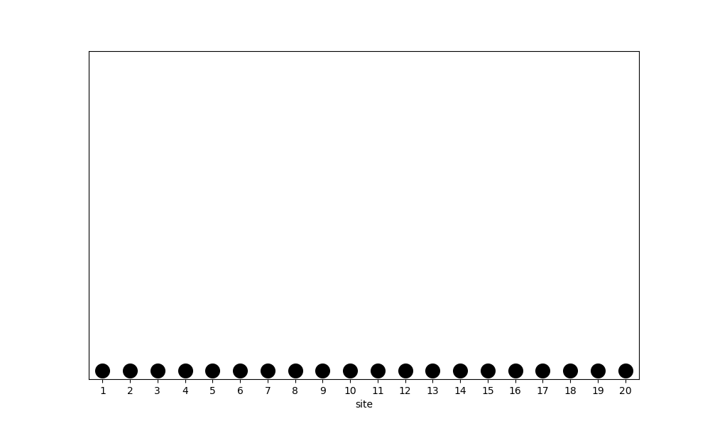
(a) $L=20$ and $n=20$

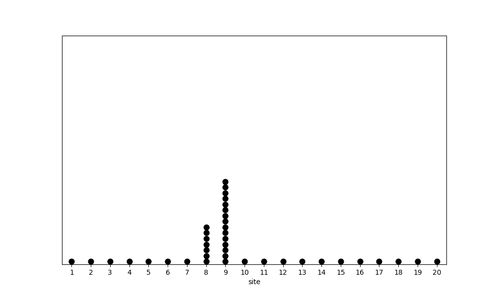
(b) $L=20$ and $n=40$

Figure 8: Snapshots for the $(0,10000,100)$ ASIP in steady state for two different systems.

5.8 $1\ll t\ll t^{n}\ll\theta$

Using (64) and simplifying

$$\varphi_{\theta,t}(\eta_{i})\approx\theta^{\eta_{i}},$$ (79)

we can write, after dropping the common factor of $\theta^{n}$ from all the weight expressions,

$$\text{wt}_{\theta,t}(\eta)\approx{\begin{bmatrix}n\\ \eta_{1},\ldots,\eta_{L}\end{bmatrix}_{\!t}}.$$ (80)

This $t-$multinomial coefficient is greatest when the particles will be maximally spread out, i.e., in the flattened configuration which was discussed in Section 5.6. Calculations for the example in (29) with the parameter values $\theta=10^{50}$ and $t=10000$ give the steady state probabilities

$$\pi(0,0,4)\approx 3.23\times 10^{-11},\pi(0,1,3)\approx 3.26\times 10^{-5},\pi(0,2,2)\approx 3.26\times 10^{-3},\pi(1,1,2)\approx 0.33.$$

See the movie t_100_theta_1e+50.mp4 among the ancillary files for a simulation of the $(0,100,10^{50})$ ASIP with $L=n=20$. A snapshot from that movie is shown in Figure 9.

Figure 9: A snapshot of the $(0,100,10^{50})$ ASIP with $L=20$ and $n=20$ in steady state.

5.9 $\theta t=1$

As calculated before in (32), we get a uniform distribution. Again, following the discussion from Section 5.2 we see that this regime shows weak condensation. Simulations in t_.01_theta_100.mp4, t_1_theta_1.mp4 and t_100_theta_.01.mp4 are added in the ancillary files for three different values of $t$ and $\theta$ where the product is $1$. Snapshots of these movies are shown in Figures 10(a), 10(b) and 10(c) respectively. For the latter, see Remark 5.1 to explain the clustering.

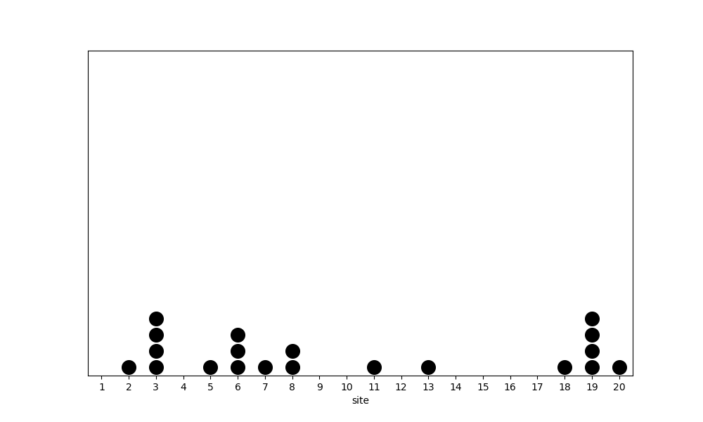
(a)

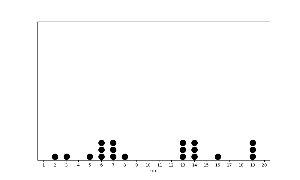
(b)

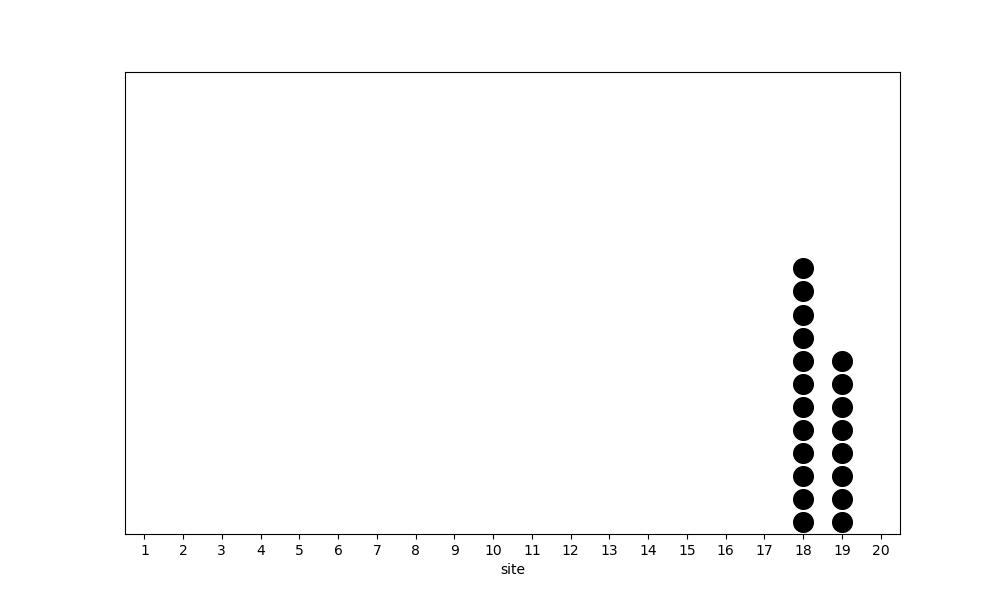
(c)

Figure 10: Snapshots for $L=20$ and $n=20$ in steady state for (a) $(0,0.01,100)$ ASIP, (b) $(0,1,1)$ ASIP and (c) $(0,100,0.01)$ ASIP.

The $\theta t=1$ curve marks a smooth crossover from the strong condensation observed when $\theta t\ll 1$ in Sections 5.1, 5.3 and 5.5 to the flattening observed when $\theta t\gg 1$ in Sections 5.4, 5.6, 5.7 and 5.8. This matches the trend observed in the variance plot shown in Figure 11.

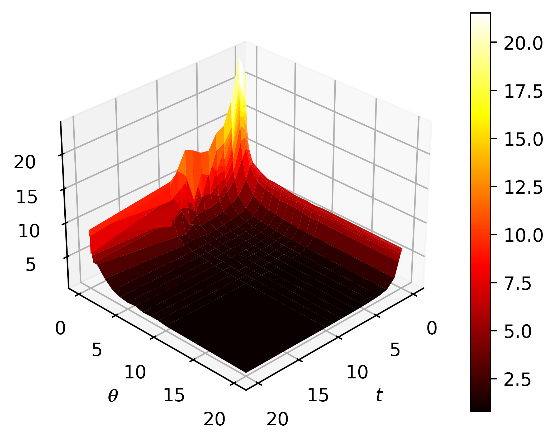
Figure 11: Variance of the single site occupation in a system with $L=6$ and $n=15$. The parameters $t,\theta$ each range over the 21 values $\{n,1/n\mid n\in\{1,\dots,10\}\}\cup\{20,1/20\}$. The variance is computed by averaging over 10000 steady state configurations for 20 different runs.

6 Palindromicity and antipalindromicity of the weights

As mentioned above, we will use the equivalent formulation of the rates in (18) and (19) when $t\neq 1$. Using the forward rate (18) in (20) for the calculation of the steady state weights, we get

$$f_{a}(m)=\prod_{i=1}^{m}\frac{u(1,i-1)}{u(i,0)}=\prod_{i=1}^{m}\frac{1-at^{i-1}}{(1-a)[i]_{t}}.$$

Recall the $t$-Pochhammer symbol given by

$$(a;t)_{m}=\prod^{m-1}_{k=0}(1-at^{k})=(1-a)(1-at)\dots(1-at^{m-1}).$$ (81)

Then we obtain, up to overall normalisation,

$$f_{a}(m)=\frac{(a;t)_{m}}{(t;t)_{m}},$$ (82)

using $(t;t)_{m}=[m]_{t}!(1-t)^{m}$. We thus obtain the steady state weight

$$\text{wt}_{a,t}(\eta)=\prod_{i=1}^{L}f_{a}(\eta_{i})=(t;t)_{n}\prod_{i=1}^{L}\frac{(a;t)_{\eta_{i}}}{(t;t)_{\eta_{i}}}$$ (83)

after rescaling. This makes all the weights polynomials in $a$ and $t$.

For example, the steady weights of the $(q,t,\theta)$ ASIP with $L=3$ and $n=4$ in (29), when rewritten in these variables, are

$$\text{wt}_{a,t}(0,0,4)= \;(1-a)(1-at)(1-at^{2})(1-at^{3}),$$ (84)

$$\text{wt}_{a,t}(0,1,3)= \;(1+t)(1+t^{2})(1-a)^{2}(1-at)(1-at^{2}),$$

$$\text{wt}_{a,t}(0,2,2)= \;(1+t^{2})(1+t+t^{2})(1-a)^{2}(1-at)^{2},$$

$$\text{wt}_{a,t}(1,1,2)= \;(1+t)(1+t^{2})(1+t+t^{2})(1-a)^{3}(1-at).$$

We denote the partition function in these variables as

$$Z^{a}_{L,n}=\sum_{\eta\in\Omega_{L,n}}\text{wt}_{a,t}(\eta).$$ (85)

Although the steady state weights factor, we do not seem to obtain simple formulas for the ordinary or exponential generating functions of $Z^{a}_{L,n}$. There is another variant, known as the Eulerian generating function [GR70] that will be useful to us. We will now show that the Eulerian generating function of the partition function is given by the product formula,

$$\sum_{n=0}^{\infty}Z^{a}_{L,n}\frac{x^{n}}{(t;t)_{n}}=\left(\frac{(ax;t)_{\infty}}{(x;t)_{\infty}}\right)^{L}.$$ (86)

To begin, we see that the generating function for $f_{a}(m)$ is

$$\sum_{m=0}^{\infty}f_{a}(m)z^{m}=\sum_{m=0}^{\infty}\frac{(a;t)_{m}}{(t;t)_{m}}z^{m}=\frac{(az;t)_{\infty}}{(z;t)_{\infty}},$$ (87)

using the general formulation of the $q$-binomial theorem [GR04, Equation (1.3.2)]. The Eulerian generating function of the partition function is then given, using (83), by

$$\sum^{\infty}_{n=0}Z^{a}_{L,n}\frac{x^{n}}{(t;t)_{n}}=\sum_{n=0}^{\infty}\left(\sum_{\eta\in\Omega_{L,n}}(t;t)_{n}\prod_{i=1}^{L}\frac{(a;t)_{\eta_{i}}}{(t;t)_{\eta_{i}}}\right)\frac{x^{n}}{(t;t)_{n}}.$$ (88)

The factor of $(t;t)_{n}$ cancels and we can split the product terms to get

$$\sum_{\eta_{1}\geq 0}\sum_{\eta_{2}\geq 0}\cdots\sum_{\eta_{L}\geq 0}\frac{(a;t)_{\eta_{1}}}{(t;t)_{\eta_{1}}}\frac{(a;t)_{\eta_{2}}}{(t;t)_{\eta_{2}}}\cdots\frac{(a;t)_{\eta_{L}}}{(t;t)_{\eta_{L}}}x^{\eta_{1}}x^{\eta_{2}}\cdots x^{\eta_{L}}.$$ (89)

Each of the $L$ sums can be performed independently using (87) to obtain (86).

We now study the symmetry properties of the steady state weights. Recall the order and degree of a polynomial defined in Section 5. One can easily compute that $\operatorname{ord}_{t}(\text{wt}_{a,t}(\eta))=\operatorname{ord}_{a}(\text{wt}_{a,t}(\eta))=0$. We begin by computing the polynomial degrees, which are crucial for establishing the symmetry properties. First, note that

$$\operatorname{deg}_{a}(a;t)_{\eta_{i}}=\eta_{i}$$

and

$$\operatorname{deg}_{t}(a;t)_{\eta_{i}}=\eta_{i}(\eta_{i}-1)/2.$$

Thus, the degree of the product of these Pochhammer terms is

$$\operatorname{deg}_{a}\Bigl(\prod_{i=1}^{L}(a;t)_{\eta_{i}}\Bigr)=\eta_{1}+\cdots+\eta_{L}=n,$$ (90)

and

$$\operatorname{deg}_{t}\Bigl(\prod_{i=1}^{L}(a;t)_{\eta_{i}}\Bigr)=\frac{\eta_{1}(\eta_{1}-1)}{2}+\cdots+\frac{\eta_{L}(\eta_{L}-1)}{2}=\frac{\eta_{1}^{2}+\cdots+\eta_{L}^{2}-n}{2}.$$ (91)

Combining these with (60) we get the degrees as

$$\operatorname{deg}_{a}(\text{wt}_{a,t}(\eta_{1},\ldots,\eta_{L}))=n,$$ (92)

and

$$\operatorname{deg}_{t}(\text{wt}_{a,t}(\eta_{1},\ldots,\eta_{L}))=\frac{n^{2}-\eta_{1}^{2}-\ldots-\eta_{L}^{2}}{2}+\frac{\eta_{1}^{2}+\ldots+\eta_{L}^{2}-n}{2}=\frac{n(n-1)}{2}.$$ (93)

Notice that the orders and degrees of $\text{wt}_{a,t}(\eta)$ in $t$ and $a$ are independent of the exact configuration $\eta$ and only depend on $n$, the total number of particles in the system. As an example, one can check that the degrees in $a$ and $t$ of steady state weights of all configurations computed in (84) are $4$ and $6$ respectively.

A polynomial $p(x)\in\mathbb{R}$ with $\operatorname{deg}_{x}(p)=d$ given by

$$p(x)=p_{0}+p_{1}x+\cdots+p_{d}x^{d},\qquad\qquad p_{d}\neq 0,$$

is said to be palindromic (resp. antipalindromic) if $p_{i}=p_{d-i}$ (resp. $p_{i}=-p_{d-i}$) for $0\leq i\leq d$. Similarly, a multivariate polynomial $p(x_{1},\dots,x_{m})$ with degrees $d_{1},\dots,d_{m}$ in the variables $x_{1},\dots,x_{m}$ respectively, is said to be palindromic (resp. antipalindromic) if the coefficient of $x_{1}^{i_{1}}\dots x_{m}^{i_{m}}$ in $p$ is the same as (resp. negative of) the coefficient of $x_{1}^{d_{1}-i_{1}}\dots x_{m}^{d_{m}-i_{m}}$ for $0\leq i_{1}\leq d_{1},\dots,0\leq i_{m}\leq d_{m}$. From the definition, the product of two palindromic polynomials is palindromic, the product of two antipalindromic polynomials is also palindromic, and the product of a palindromic and antipalindromic polynomial is antipalindromic.

We will now show that $\text{wt}_{a,t}(\eta)$ is a palindromic or antipalindromic polynomial in the variables $t$ and $a$ according to whether $n$ is even or odd. We have already shown in [AM24, Equation (4.3)] that the $t$-binomial coefficient is palindromic as a function of $t$. Since the $t$-multinomial coefficient can be expressed as a product of $t$-binomial coefficients, it is also palindromic. Thus, it remains to look at the product of the Pochhammer symbols.

Consider a single Pochhammer factor $(a;t)_{m}$ and look at its expansion,

$$(a;t)_{m}=\prod^{m-1}_{k=0}(1-at^{k})=(1-a)(1-at)\ldots(1-at^{m-1}).$$

There are $m$ factors, each containing two terms. Thus, each term $T$ in the expansion of this product can be represented as a binary vector $b=(b_{1},\dots,b_{m})\in\{0,1\}^{m}$, where $b_{i}=0$ means the term $1$ is chosen from the $i$’th factor and $b_{i}=1$ means the term $-at^{i-1}$ is chosen. Clearly, the sign of $T$ is the parity of the number of positions $i$ such that $b_{i}=1$. Let $\bar{b}=(1-b_{1},\dots,1-b_{m})$, with corresponding term in the expansion denoted $\overline{T}$. Then, the sign of $\overline{T}$ is the same as that of $T$ if $m$ is even and the opposite of that when $m$ is odd. Moreover, it is easy to check that $\operatorname{deg}_{a}(\overline{T})+\operatorname{deg}_{a}(T)=m$ and $\operatorname{deg}_{t}(\overline{T})+\operatorname{deg}_{t}(T)=m(m-1)/2$. Therefore, $(a;t)_{m}$ is palindromic if $m$ is even and and antipalindromic if $m$ is odd.

Now consider $\prod_{i=1}^{L}(a;t)_{\eta_{i}}$. If $n$ is even, then the number of $i$’s where $\eta_{i}$ is odd is also even and therefore the product becomes palindromic. Similarly, if $n$ is odd, the number of $i$’s where $\eta_{i}$ is odd is also odd and therefore the product becomes antipalindromic. Therefore $\text{wt}_{a,t}(\eta)$ is palindromic if $n$ is even and antipalindromic if $n$ is odd.

We can check this for the example in (84). A nice way of visualizing coefficients of two-variable polynomials is by arranging the coefficients as a matrix. For each configuration $\eta$, we write the matrix whose $(i,j)$’th entry is the coefficient of $a^{i-1}t^{j-1}$ below.

$$(0,0,4):\begin{pmatrix}1&0&0&0&0&0&0\\ -1&-1&-1&-1&0&0&0\\ 0&1&1&2&1&1&0\\ 0&0&0&-1&-1&-1&-1\\ 0&0&0&0&0&0&1\end{pmatrix},$$

$$(0,1,3):\begin{pmatrix}1&1&1&1&0&0&0\\ -2&-3&-4&-4&-2&-1&0\\ 1&3&5&6&5&3&1\\ 0&-1&-2&-4&-4&-3&-2\\ 0&0&0&1&1&1&1\end{pmatrix},$$

$$(0,2,2):\begin{pmatrix}1&1&2&1&1&0&0\\ -2&-4&-6&-6&-4&-2&0\\ 1&5&7&10&7&5&1\\ 0&-2&-4&-6&-6&-4&-2\\ 0&0&1&1&2&1&1\end{pmatrix}$$

and

$$(1,1,2):\begin{pmatrix}1&2&3&3&2&1&0\\ -3&-7&-11&-12&-9&-5&-1\\ 3&9&15&18&15&9&3\\ -1&-5&-9&-12&-11&-7&-3\\ 0&1&2&3&3&2&1\end{pmatrix}.$$

In each case, the matrix is invariant under a rotation of $180$ degrees.

For comparison, we also demonstrate the antipalindromic case with odd number of particles. Consider the system with $L=3$ and $n=3$. The matrices from the steady state weights are given by

$$(0,0,3):\begin{pmatrix}1&0&0&0\\ -1&-1&-1&0\\ 0&1&1&1\\ 0&0&0&-1\end{pmatrix},\quad(0,1,2):\begin{pmatrix}1&1&1&0\\ -2&-3&-3&-1\\ 1&3&3&2\\ 0&-1&-1&-1\end{pmatrix},$$

and

$$(1,1,1):\begin{pmatrix}1&2&2&1\\ -3&-6&-6&-3\\ 3&6&6&3\\ -1&-2&-2&-1\end{pmatrix}.$$

For all of these matrices, a rotation by $180$ degrees negates the matrix.

7 Enriched process for $t=1$ and $\theta\in\mathbb{N}$

In this section, we define a new class of particle systems which projects to the $(q,t,\theta)$ ASIP and when $t=1$ and $\theta$ takes integer values.

We will define the enriched ASIP on configurations consisting of three kinds of objects. We have integers labelled $1$ through $n$, $L(\theta-1)$ identical dots $\bullet$, and $L-1$ separators denoted by $\mid$. Thus, each configuration has length $L+n-1$. Further, we enforce the condition that there are $\theta-1$ $\bullet$’s between any two successive separators in each configuration. We will think of these configurations as embedded in a circle with a separator between the first and the last object. To avoid cluttering the notation, we will not depict this separator. We will denote by $\widehat{\Omega}^{\theta}_{L,n}$ the configuration space of the enriched ASIP. It is not difficult to see that the cardinality of this set is

$$|\widehat{\Omega}^{\theta}_{L,n}|=\frac{(n+L\theta-1)!}{(L\theta-1)!}=n!\,\binom{n+L\theta-1}{n}.$$

As an example, the set of configurations for $L=3$, $n=2$ and $\theta=2$ is

$$\widehat{\Omega}^{2}_{3,\;2}=\left\{\begin{split}\;\bullet\mid\bullet\mid\bullet\;1\;2,\;\bullet\mid\bullet\mid\bullet\;2\;1,\;\bullet\mid\bullet\mid 1\bullet 2,\;\bullet\mid\bullet\mid 1\;2\;\bullet,\;\bullet\mid\bullet\mid 2\bullet 1,\;\bullet\mid\bullet\mid 2\;1\;\bullet\\ \;\bullet\mid\bullet\;1\mid\bullet\;2,\;\bullet\mid\bullet\;1\mid 2\;\bullet,\;\bullet\mid\bullet\;1\;2\mid\bullet,\;\bullet\mid\bullet\;2\mid\bullet\;1,\;\bullet\mid\bullet\;2\mid 1\;\bullet,\;\bullet\mid\bullet\;2\;1\mid\bullet\\ \;\bullet\mid 1\;\bullet\mid\bullet\;2,\;\bullet\mid 1\;\bullet\mid 2\;\bullet,\;\bullet\mid 1\bullet 2\mid\bullet,\;\bullet\mid 1\;2\;\bullet\mid\bullet,\;\bullet\mid 2\;\bullet\mid\bullet\;1,\;\bullet\mid 2\;\bullet\mid 1\;\bullet\\ \;\bullet\mid 2\;\bullet\;1\mid\bullet,\;\bullet\mid 2\;1\;\bullet\mid\bullet,\;\bullet\;1\mid\bullet\mid\bullet\;2,\;\bullet\;1\mid\bullet\mid 2\;\bullet,\;\bullet\;1\mid\bullet\;2\mid\bullet,\;\bullet\;1\mid 2\;\bullet\mid\bullet\\ \;\bullet\;1\;2\mid\bullet\mid\bullet,\;\bullet\;2\mid\bullet\mid\bullet\;1,\;\bullet\;2\mid\bullet\mid 1\;\bullet,\;\bullet\;2\mid\bullet\;1\mid\bullet,\;\bullet\;2\mid 1\;\bullet\mid\bullet,\;\bullet\;2\;1\mid\bullet\mid\bullet\\ \;1\;\bullet\mid\bullet\mid\bullet\;2,\;1\;\bullet\mid\bullet\mid 2\;\bullet,\;1\;\bullet\mid\bullet\;2\mid\bullet,\;1\;\bullet\mid 2\;\bullet\mid\bullet,\;1\;\bullet\;2\mid\bullet\mid\bullet,\;1\;2\;\bullet\mid\bullet\mid\bullet\\ \;2\;\bullet\mid\bullet\mid\bullet\;1,\;2\;\bullet\mid\bullet\mid 1\;\bullet,\;2\;\bullet\mid\bullet\;1\mid\bullet,\;2\;\bullet\mid 1\;\bullet\mid\bullet,\;2\;\bullet\;1\mid\bullet\mid\bullet,\;2\;1\;\bullet\mid\bullet\mid\bullet\end{split}\right\}.$$ (94)

7.1 Dynamics

In this enriched ASIP, we let the particles hop around while the dots and separators remain stationary. The only hops that are allowed are those where a particle hops over a single separator to its right (resp. left) with rate $1$ (resp. with rate $q$) and inserts itself between any two objects. Since the enriched ASIP is periodic, particles before the first separator can jump to locations after the last separator with rate $q$, and similarly particles after the last separator can jump to locations before the first separator with rate $1$. Examples of allowed transitions are

$$(\;\bullet\;\underline{2}\mid\bullet\mid\bullet\mid 1\;\bullet\;)\xrightarrow[]{q}(\;\bullet\mid\bullet\mid\bullet\mid 1\;2\;\bullet\;)$$

and

$$(\;\bullet\;2\mid\bullet\mid\bullet\mid\underline{1}\;\bullet\;)\xrightarrow[]{1}(\;1\;\bullet\;2\mid\bullet\mid\bullet\mid\bullet\;),$$

where the particle moving is underlined. We illustrate all incoming and outgoing transitions for the chosen state $(\;\bullet\mid 1\;\bullet\mid\bullet\;2\;)$ in Figure 12.

Figure 12: All allowed incoming and outgoing transitions for state $(\;\bullet\mid 1\;\bullet\mid\bullet\;2\;)$ with their respective rates. The particle involved in the transition is underlined.

7.2 Steady state for the enriched ASIP

We begin by proving that this process is ergodic. We want to show that we can go from any given state to any other state in a finite number of moves. To do this, we deploy the following algorithm. Starting from a given state $\hat{\eta}\in\widehat{\Omega}^{\theta}_{L,n}$, we can move the particle $1$ across separators until it is at the leftmost position of the configuration. We can then move the particle $2$ immediately to the right of the particle $1$, and continuing this for all the numbered particles, one obtains the configuration

$$\hat{c}=(1\;2\;\ldots\;n\;\bullet\cdots\bullet\mid\bullet\cdots\bullet\mid\dots\mid\bullet\cdots\bullet).$$

Now, starting from $\hat{c}$, it is easy to create any other state by sequentially sending the numbered particles starting from the highest to the lowest to their required positions in a sequence of rightward jumps as per the desired state, thus proving ergodicity.

Since the enriched ASIP is ergodic, the steady state is unique. We now show that it is uniform, i.e.

$$\text{wt}_{\theta,t}(\hat{\eta})=1,$$ (95)

for any $\hat{\eta}\in\widehat{\Omega}^{\theta}_{L,n}$. To prove this, it will suffice to show that the sum of the rates of incoming and outgoing transitions to any state are the same. In Figure 12 for example, this sum is $5+5q$.

Fix a configuration $\hat{\eta}$. Fix an integer $i$, $1\leq i\leq L$. We will analyse the transitions of $\hat{\eta}$ that lead to changes between the $(i-1)$’th separator and the $i$’th separator, where the $0$’th separator is the one between the first and last object (which we omit in our notation). Suppose there are $p$ particles between these separators labelled $\alpha_{1},\alpha_{2},\ldots,\alpha_{p}$ from left to right. Similarly let $(\gamma_{1},\gamma_{2},\ldots,\gamma_{m})$ be the particles between the $(i-2)$’th separator and the $(i-1)$’th separator and $(\beta_{1},\beta_{2},\ldots,\beta_{r})$ be the particles between the $i$’th separator and $(i+1)$’th separator, so that $\hat{\eta}$ looks like

$$\hat{\eta}=\ldots\underset{\underset{i-2}{\downarrow}}{\mid}\ldots,\gamma_{1},\ldots,\gamma_{m},\ldots\underset{\underset{i-1}{\downarrow}}{\mid}\ldots,\alpha_{1},\ldots,\alpha_{p},\ldots\underset{\underset{i}{\downarrow}}{\mid}\ldots,\beta_{1},\ldots,\beta_{r},\ldots\underset{\underset{i+1}{\downarrow}}{\mid}\ldots\;.$$ (96)

We first analyse the forward transitions between these consecutive separators. For the outgoing transitions, each particle labelled $\alpha$ can jump to the right across the $i$’th separator. Since there are $\theta-1$ dots and $r$ particles labelled $\beta$ there, we get $r+\theta$ available spaces to transition to. Since the rate for each forward transition is $1$ and there are $p$ particles labelled $\alpha$, we get the total outgoing rate in the forward direction to be $p(r+\theta)$. Similarly, the total outgoing rate in the reverse direction is $qp(m+\theta)$, as the rate for each reverse transition is $q$. Now each of the outgoing transitions can be reversed with the rates flipped, so that the total incoming rate into $\hat{\eta}$ involving particles labelled $\alpha$ being $qp(r+\theta)$ in the reverse direction and $p(m+\theta)$ in the forward direction.

Now, let us sum the total incoming and outgoing transition rates. For convenience, let the number of particles between the $(i-1)$’th and $i$’th separators be $\eta_{i}$ for $1\leq i\leq L$. Then the total number of forward outgoing transitions from $\hat{\eta}$ is

$$\sum_{i=1}^{L}\eta_{i}(\eta_{i+1}+\theta)=\sum_{i=1}^{L}\left(\eta_{i}\eta_{i+1}+\theta\,n\right).$$ (97)

Similarly, the total number of forward incoming transitions into $\hat{\eta}$ is

$$\sum_{i=1}^{L}\eta_{i}(\eta_{i-1}+\theta)=\sum_{i=1}^{L}\left(\eta_{i}\eta_{i-1}+\theta\,n\right).$$ (98)

The number of transitions obtained in (97) and (98) are clearly the same due to periodic boundary conditions. By an identical argument, one can show that the total weight of reverse outgoing transitions equals that of reverse incoming transitions. Thus, the uniform distribution proposed in (95) satisfies the master equation.

7.3 Proof of projection

We will now show that the enriched ASIP defined in Section 7 projects to the $(q,t,\theta)$ ASIP. To that end, define $\Pi:\widehat{\Omega}_{L,n}^{\theta}\to\Omega_{L,n}$ by

$$\Pi(\hat{\eta})=(m_{1},\dots,m_{L}),$$ (99)

where $m_{i}$ counts the number of numbered particles between $(i-1)$’th and $i$’th separator. For the example of $\widehat{\Omega}_{3,2}^{2}$ shown in (94), we have

$$\Pi^{-1}(\{(1,0,1)\})=\{\;1\;\bullet\mid\bullet\mid 2\;\bullet\;,\quad\bullet\;1\mid\bullet\mid 2\;\bullet\;,\quad 1\;\bullet\mid\bullet\mid\bullet\;2\;,\quad\bullet\;1\mid\bullet\mid\bullet\;2\;,\\ 2\;\bullet\mid\bullet\mid 1\;\bullet\;,\quad\bullet\;2\mid\bullet\mid 1\;\bullet\;,\quad 2\;\bullet\mid\bullet\mid\bullet\;1\;,\quad\bullet\;2\mid\bullet\mid\bullet\;1\;\}.$$ (100)

We also define the rate from an enriched state to a projected state as

$$\textrm{rate}(\hat{\eta}\rightarrow m)=\sum_{\hat{\tau}\in\Pi^{-1}(m)}\textrm{rate}(\hat{\eta}\rightarrow\hat{\tau}).$$ (101)

To prove this projection, we need to show the lumping property [LPW09, Lemma 2.5]

$$\textrm{rate}(\hat{\eta}_{1}\rightarrow m^{\prime})=\textrm{rate}(\hat{\eta}_{2}\rightarrow m^{\prime})\quad\forall\,\hat{\eta}_{1},\hat{\eta}_{2}\in\Pi^{-1}(m),$$ (102)

for all $m,m^{\prime}\in\Omega_{L,n}$. Moreover, we have to show that this rate is the same as $\textrm{rate}(m\rightarrow m^{\prime})$ for the $(q,t,\theta)$ ASIP.

Let $m,m^{\prime}\in\Omega_{L,n}$ such that a particle crosses the $i$’th separator in $m$ to reach $m^{\prime}$, namely a forward transition. Then $m^{\prime}_{i}=m_{i}-1$, $m^{\prime}_{i+1}=m_{i}+1$, and $m^{\prime}_{j}=m_{j}$ for all $j\neq i,i+1$. Let $\hat{\eta}\in\widehat{\Omega}_{L,n}^{\theta}$ such that $\Pi(\hat{\eta})=m$. Then any transition that involves a particle between the $(i-1)$’th and $i$’th separators moving in the forward direction leading to a configuration $\hat{\eta}^{\prime}$ satisfies the property that $\Pi(\hat{\eta}^{\prime})=m^{\prime}$. As we have shown in Section 7.2, the total sum of these rates is $\eta_{i}(\eta_{i+1}+\theta)$, which is also $\textrm{rate}(m\rightarrow m^{\prime})$ in the $(q,t,\theta)$ ASIP. A similar argument goes through for reverse transitions, completing the proof of projection.

It is a standard result that if a Markov process projects onto another Markov process, then the steady state of the latter can be obtained by summing over the steady state probabilities of the former. In the case when $\theta$ is a positive integer, we can compute the steady state weights of the $(q,t,\theta)$ ASIP using the enriched ASIP. Since the steady state weights of the enriched ASIP are equal to $1$, $\text{wt}_{\theta,t}(m)=\bigm|\Pi^{-1}(m)\bigm|$. To find this, we first place $m_{i}$ particles between the $(i-1)$’th and $i$’th separator for each $i$ in

$$\binom{n}{m_{1},\ldots,m_{L}}$$

ways. Now, these $m_{i}$ particles have to be placed along with the $\theta-1$ dots there. This can be done in

$$\prod_{i=1}^{L}\frac{(m_{i}+\theta-1)!}{(\theta-1)!}$$

ways. Multiplying these factors gives us the steady state weight formula found previously in (36) up to the constant $1/((\theta-1)!)^{L}$.

Recall that the Markov chain tree theorem [LR83, AT89] expresses the steady state weights as polynomials in the rates. For us, when $t=1$, these are therefore polynomials in $\theta$ alone. We have so far given an alternate proof for the steady state distribution at $t=1$ and all integer values of $\theta$, which are of course infinitely many. Since we have shown that these steady state weights coincide for infinitely many values of $\theta$, it follows that the steady state for the $(q,1,\theta)$ ASIP given by (36) is correct as a function of $\theta$.

References

- [AM24] Arvind Ayyer and Samarth Misra. An exactly solvable asymmetric k-exclusion process. Journal of Physics A: Mathematical and Theoretical, 57, 07 2024.
- [AT89] Venkat Anantharam and Pantelis Tsoucas. A proof of the markov chain tree theorem. Statistics & Probability Letters, 8(2):189–192, 1989.
- [CCG14] Jiarui Cao, Paul Chleboun, and Stefan Grosskinsky. Dynamics of condensation in the totally asymmetric inclusion process. Journal of Statistical Physics, 155(3):523–543, 2014.
- [Com74] Louis Comtet. Advanced Combinatorics. D. Reidel Publishing Company, Boston, 1974.
- [CT85] Christiane Cocozza-Thivent. Processus des misanthropes. Z. Wahrsch. Verw. Gebiete, 70(4):509–523, 1985.
- [EW14] M R Evans and B Waclaw. Condensation in stochastic mass transport models: beyond the zero-range process. Journal of Physics A: Mathematical and Theoretical, 47(9):095001, feb 2014.
- [Gil76] Daniel T Gillespie. A general method for numerically simulating the stochastic time evolution of coupled chemical reactions. Journal of computational physics, 22(4):403–434, 1976.
- [GKR07] Cristian Giardinà, Jorge Kurchan, and Frank Redig. Duality and exact correlations for a model of heat conduction. Journal of Mathematical Physics, 48(3):033301, 03 2007.
- [GKRV09] Cristian Giardinà, Jorge Kurchan, Frank Redig, and Kiamars Vafayi. Duality and hidden symmetries in interacting particle systems. Journal of Statistical Physics, 135(1):25–55, 2009.
- [GR70] Jay Goldman and Gian-Carlo Rota. On the foundations of combinatorial theory. IV. Finite vector spaces and Eulerian generating functions. Studies in Appl. Math., 49:239–258, 1970.
- [GR04] George Gasper and Mizan Rahman. Basic hypergeometric series, volume 96 of Encyclopedia of Mathematics and its Applications. Cambridge University Press, Cambridge, second edition, 2004. With a foreword by Richard Askey.
- [GRV10] C. Giardinà, F. Redig, and K. Vafayi. Correlation inequalities for interacting particle systems with duality. Journal of Statistical Physics, 141:242–263, 2010.
- [GRV11] Stefan Grosskinsky, Frank Redig, and Kiamars Vafayi. Condensation in the inclusion process and related models. Journal of Statistical Physics, 142(5):952–974, 2011.
- [JKK05] Norman L. Johnson, Adrienne W. Kemp, and Samuel Kotz. Univariate discrete distributions. Wiley Series in Probability and Statistics. Wiley-Interscience [John Wiley & Sons], Hoboken, NJ, third edition, 2005.
- [Lan19] Claudio Landim. Metastable Markov chains. Probab. Surv., 16:143–227, 2019.
- [LPW09] David A. Levin, Yuval Peres, and Elizabeth L. Wilmer. Markov chains and mixing times. American Mathematical Society, Providence, RI, 2009. With a chapter by James G. Propp and David B. Wilson.
- [LR83] Frank Thomson Leighton and Ronald L Rivest. The Markov chain tree theorem. Massachusetts Institute of Technology, Laboratory for Computer Science, 1983.