Pauli Propagation: Simulating Quantum Spin Dynamics via Operator Complexity

Abstract

Simulating real-time quantum dynamics in interacting spin systems is a fundamental challenge, where exact diagonalization suffers from exponential Hilbert-space growth and tensor-network methods face entanglement barriers. In this work, we introduce a scalable Pauli propagation approach that evolves local observables directly in the Heisenberg picture. Theoretically, we derive a priori error bounds governed by the Operator Stabilizer Rényi entropy (OSE) $\mathcal{S}^{\alpha}(O)$, which explicitly links the truncation accuracy to operator complexity and prescribes a suitable Top-$K$ truncation strategy. For the 1D Heisenberg model with $J_{z}=0$, we prove the number of non-zero Pauli coefficients scales quadratically in Trotter steps, establishing the compressibility of Heisenberg-evolved operators. Numerically, we validate the framework on XXZ Heisenberg chain benchmarks, showing high accuracy with small $K$ in free regimes ($J_{z}=0$) and competitive performance against tensor-network methods (e.g., TDVP) in interacting cases ($J_{z}=0.5$). These results establish an observable-centric simulator whose cost is governed by operator complexity rather than entanglement, offering a practical alternative for studying non-equilibrium dynamics in quantum many-body systems.

I Introduction

Simulating real-time quantum dynamics in interacting many-body systems represents a fundamental challenge across condensed matter physics [1, 2, 3, 4], quantum information science [5, 6, 7, 8, 9], and statistical mechanics [10, 11, 12, 13, 14]. Understanding non-equilibrium phenomena such as thermalization [15, 14, 11, 12], information scrambling [16, 17, 18], and transport properties requires accurate numerical methods for evolving quantum states or observables in time [19, 20].

However, the exponential growth of Hilbert space dimension severely constrains classical simulations [21, 22, 23, 24]. Traditional approaches face critical limitations: Exact diagonalization is restricted to small systems by memory constraints, while tensor network methods encounter barriers with the rapid growth of entanglement entropy in generic quenched dynamics [25, 26, 27, 28, 29]. This entanglement barrier fundamentally restricts the simulation timescales for density matrix renormalization group (DMRG) [30, 31, 32] and time-dependent variational principle (TDVP) [33, 34, 35] approaches, particularly in higher dimensions or in systems undergoing information scrambling [36, 37, 38, 29].

Recent advances in Pauli-based simulating approach for quantum circuits reveal a promising alternative. By targeting specific observables rather than states, techniques developed for simulating noisy quantum circuits have demonstrated that these methods can outperform tensor networks in certain regimes [39, 40, 41, 42, 43, 44, 45, 46, 47, 48]. This motivates our operator-centric approach to Hamiltonian dynamics in the Heisenberg picture, focusing on the evolution of operators rather than states.

In this work, we develop a scalable Pauli propagation framework for simulating the real-time evolution of local observables in spin systems. The key idea is to Trotterize the unitary evolution and back-propagate each observable’s Pauli component through the sequence of elementary evolutions. The key insight is that each single-Pauli term acts linearly on the Pauli basis with a closed form. This enables sparse, structure-preserving updates to the observable’s Pauli expansion.

To control the combinatorial growth of Pauli terms, we introduce Top-$K$ truncation strategy that retains $K$ dominant coefficients at each evolution step, followed by norm renormalization for stability. The simulator’s cost thus depends on the compressibility of the Heisenberg-evolved observable rather than the entanglement of the evolving state.

A key theoretical contribution of our work is the derivation of a priori error bounds that link truncation accuracy to an intrinsic measure of operator complexity, the Operator Stabilizer Rényi entropy (OSE) [49]. We prove that the error incurred by the Top-$K$ truncation strategy decays at a rate controlled by OSE. This provides explicit resource prescriptions for choosing a proper $K$ to meet a target accuracy. Conceptually, the OSE plays the role dual to the Stabilizer Rényi entropies used for states [50], formalizing the intuition that observables with low Pauli entropy remain highly compressible under Heisenberg evolution.

We demonstrate that the Pauli basis decomposition intrinsically curbs the growth of operator support in paradigmatic models. For the 1D XY Heisenberg chain, the number of non-zero Pauli coefficients generated from a local $(Z_{l})$ grows only quadratically with the number of Trotter steps, i.e., $\order{s^{2}}$. This explains the sustained effectiveness of aggressive truncation even at late times and provides a concrete example where operator-complexity-based approaches could outperform those based on state entanglement. Furthermore, this conclusion is supported by numerical experiments.

Numerically, we validate our approach on 1D Heisenberg chain benchmarks relevant to non-equilibrium dynamics. In free regimes, our method achieves exact accuracy with a small number of retained Pauli coefficients $K$. The computational resources required to maintain a fixed accuracy scale merely linearly with the simulated time, This favorable scaling stems from the slow growth of operator complexity under time evolution, as captured by OSE. This contrasts sharply with state-based methods whose memory usage grows exponentially with entanglement. In interacting cases, where $J_{z}\neq 0$, our approach remains competitive with tensor-network time evolution methods. These results establish an observable-centric simulation paradigm whose cost is governed by operator complexity rather than entanglement, offering a practical alternative for studying non-equilibrium dynamics in quantum many-body systems.

Our results connect and extend recent advances in Pauli propagation for quantum circuits to Hamiltonian time evolution of lattice models, providing: (i) a practical algorithm with simple truncations, (ii) entropy-based error guarantees, and (iii) model-specific structure theorems that explain compressibility in local spin systems. Our approach establishes an operator-centric alternative to state-based simulators, with cost governed by operator complexity rather than entanglement, offering a practical pathway for studying non-equilibrium dynamics in quantum many-body systems.

The following section is organized as follows: Sec. II details our method and algorithmic implementation, Sec. III presents analytical error bounds based on OSE, Sec. IV contains numerical benchmarks on Heisenberg models, and Sec. V provides conclusions and future directions.

II Pauli Propagation Method

Consider $d\rho/dt=-i[H,\rho]$ with a Pauli decomposition $H=\sum_{i=1}^{N_{H}}w_{i}P_{i},\;P_{i}\in\{\mathbb{I},X,Y,Z\}^{\otimes n}$, where $N_{H}$ is the number of Pauli words $P_{i}$ and $n$ is the system size, $w_{i}$ are the Pauli coefficients. The density matrix evolves as

$$\rho(t)=\text{exp}\left(-iHt\right)\,\rho(0)\,\text{exp}\left(iHt\right).$$ (1)

Using the Trotter decomposition with $\tau=t/N$, there is:

$$\text{exp}\left(-iHt\right)=\prod_{s=1}^{N}\prod_{i=1}^{N_{H}}\text{exp}\left(-iw_{i}P_{i}\tau\right)+\mathcal{O}(\tau^{2}).$$ (2)

Thus, the density matrix at time $t$ can be approximated as:

$$\rho(t)\approx\left[\prod_{s=1}^{N}U(\tau)\right]\rho(0)\left[\prod_{s=1}^{N}U(\tau)\right]^{\dagger},$$ (3)

where $U(\tau):=\prod_{i=1}^{N_{H}}\text{exp}\left(-iw_{i}P_{i}\tau\right)$ is the Trotterized evolution operator for a single time step.

For an observable $O=\sum_{j}c_{j}P_{j}$, we could calculate the expectation value $\langle O\rangle_{\rho(t)}=\tr{O\rho(t)}$ by back-propagating those Pauli words $P_{j}$ in the Heisenberg picture under Pauli evolution.

Let $\vec{O}=(O_{0},O_{1},\ldots,O_{N})$ denote the evoluted trajectory of $O$ under reverse order of time. Therefore, $O_{N}=O$ and $O_{N-1},O_{N-2},\ldots,O_{0}$ defined recursively. That is, for step $s$, we have $O_{s}=\sum_{j}c_{s,j}P_{s,j}$ with $c_{s,j}=\frac{1}{2^{n}}\tr{P_{s,j}O_{s}}$, then the next operator:

$$O_{s-1} =U(\tau)^{\dagger}O_{s}U(\tau)$$ (4)

$$=\sum_{j}c_{s,j}U(\tau)^{\dagger}P_{s,j}U(\tau).$$

Consequently, calculating the expectation value of $O$ at time $t$ is now related to calculating the final operator $O_{0}$:

$$\langle O\rangle_{\rho(t)}\approx\tr{O\prod_{s=1}^{N}U(\tau)\rho(0)\prod_{s=1}^{N}{U(\tau)}^{\dagger}}=\tr{O_{0}\rho(0)},$$ (5)

For a single pair of Pauli words $(P_{s,j},P_{i})$, we noticed the closed form:

$$\left[\text{exp}\left(-iw_{i}P_{i}\tau\right)\right]^{\dagger}P_{s,j}\left[\text{exp}\left(-iw_{i}P_{i}\tau\right)\right]$$ (6)

$$=,$$

which can be calculated in $\order{n}$ by checking the commutation relation.

However, naively employing Eq. (6) to Eq. (4) would cause $\absolutevalue{O_{s-1}}$ to grow combinatorially as $\order{2^{N_{H}}\absolutevalue{O_{s}}}$, where $\absolutevalue{O_{s}}$ denotes the number of terms in $O_{s}$, making the computation infeasible.

To address this issue, we introduced the Top-$K$ truncation strategy at each step: given a threshold $K$, retain only $K$ coefficients with largest magnitude in $O_{s}=\sum_{j}c_{s,j}P_{s,j}$ and define:

$$\widehat{O}_{s}=\sum_{j=1}^{K}c_{s,j}^{\prime}P_{s,j}^{\prime},$$ (7)

where $\{c_{s,j}^{\prime}\}_{j=1}^{K}$ are the selected $K$ coefficients and $\{P_{s,j}^{\prime}\}_{j=1}^{K}$ are the associated Pauli words. We denote the resulting truncated observable sequence by $\{\widehat{O}_{s}\}_{s=0}^{N}$. Under this scheme, the total cost is $\order{nNN_{H}K}$.

Additionally, after truncation, we rescale $\widehat{O}_{0}$ to match the Hilbert-Schmidt norm of $O_{0}$:

$$\widehat{O}_{0}\leftarrow\widehat{O}_{0}\times\frac{\norm{O}_{2}}{\norm{\widehat{O}_{0}}_{2}},$$ (8)

such that $\norm{\widehat{O}_{0}}_{2}=\norm{O_{0}}_{2}$. Finally, we approximate the $\langle O\rangle_{\rho(t)}$ by $\langle\widehat{O}\rangle_{\rho(t)}=\tr{\widehat{O}_{0}\rho(0)}$.

The above procedure is summarized as Algorithm 1. More details are provided in Appendix A.

In addition to Top-$K$ truncation, another common truncation strategy in Pauli-based simulations is Hamming weight truncation [39, 40, 42, 43, 44, 45, 47], which retains only Pauli terms with lower Hamming weight. We also investigate this strategy and find that it is unnecessary in Heisenberg model simulations, see Appendix F.

Input: Hamiltonian $H$, initial state $\rho(0)$, observable $O$, time $t$, number of time steps $N$, term budget $K$

Output: Approximated observable value $\langle\hat{O}\rangle_{\rho(t)}$

Set $\tau\leftarrow t/N$;

Set $\widehat{O}_{N}\leftarrow O$;

for $s$ from $N$ to $1$ do

    Set $\widehat{O}_{s-1}\leftarrow\widehat{O}_{s}$;

   

   for $i$ in $1,\ldots,N_{H}$ do

       Set $O_{\text{Temp}}\leftarrow 0$;

      

      forall Pauli terms $P_{\alpha}$ in $\widehat{O}_{s-1}=\sum_{\alpha}c_{\alpha}P_{\alpha}$ do

          Set $O_{\text{Temp}}\leftarrow O_{\text{Temp}}+\text{exp}\left(-iw_{i}P_{i}\tau\right)^{\dagger}P_{\alpha}\text{exp}\left(-iw_{i}P_{i}\tau\right)$;

         

       end forall

      

      Set $O_{\text{Temp}}\leftarrow\text{Top-}K\text{ terms by }|c_{\alpha}|\text{ from }O_{\text{Temp}}$;

      

      Set $\widehat{O}_{s-1}\leftarrow O_{\text{Temp}}$;

      

    end for

   

end for

Set $\widehat{O}_{0}\leftarrow\widehat{O}_{0}\times\frac{\norm{O}_{2}}{\norm{\widehat{O}_{0}}_{2}}$;

Set $\langle\hat{O}\rangle_{\rho(t)}\leftarrow\tr{\widehat{O}_{0}\rho(0)}$;

return $\langle\hat{O}\rangle_{\rho(t)}$;

Algorithm 1 Pauli Propagation for Real-time Evolution

III Analytical Bounds

In this section, we provide analytical bounds on the error of the Top-$K$ truncation strategy. Firstly, we introduce the OSE, an intrinsic measure of the complexity of an operator in the Pauli basis.

Definition 1 (Operator Stabilizer Rényi entropy [49]).

Let $O$ be an operator on $n$ qubits with Pauli coefficients $c_{i}=\frac{1}{2^{n}}\tr{P_{i}O}$ for $P_{i}\in\{I,X,Y,Z\}^{\otimes n}$, and denote the squared coefficients by $\bm{c^{2}}=(c_{1}^{2},c_{2}^{2},\ldots)$. For $\alpha>0$, $\alpha\neq 1$, the Operator Stabilizer Rényi entropy (OSE) of $O$ is defined as:

$$\mathcal{S}^{\alpha}(O)\coloneqq\frac{\alpha}{1-\alpha}\,\ln{\norm{\bm{c^{2}}}_{\alpha}},$$ (9)

where $\norm{\bm{c^{2}}}_{\alpha}=\left(\sum_{i=1}^{\infty}c_{i}^{2\alpha}\right)^{\frac{1}{\alpha}}$.

This quantity can be viewed as the adjoint analogue of the stabilizer Rényi entropy [50], acting on observables rather than states. Like its state counterpart, OSE quantifies the ”non-stabilizerness” or ”magic” of an operator. A resource theory framework is established for OSE [49]. The following lemma records several basic properties of OSE:

Lemma 1.

The OSE $\mathcal{S}^{\alpha}(O)$ satisfies the following properties:

1. $\mathcal{S}^{\alpha}(O_{1}\otimes O_{2})=\mathcal{S}^{\alpha}(O_{1})+\mathcal{S}^{\alpha}(O_{2})$.

2. For a Clifford circuit $U$, we have $\mathcal{S}^{\alpha}(UOU^{\dagger})=\mathcal{S}^{\alpha}(O)$.

3. For $0<\alpha<0.5$, $\mathcal{S}^{\alpha}(O)$ is concave, i.e., for any $\sum_{i}\lambda_{i}=1$ with $\lambda_{i}\geq 0$, we have $\mathcal{S}^{\alpha}(\sum_{i}\lambda_{i}O_{i})\geq\sum_{i}\lambda_{i}\mathcal{S}^{\alpha}(O_{i})$.

4. For $0.5\leq\alpha<1$, $\text{exp}\left(\mathcal{S}^{\alpha}(O)\right)$ is convex, i.e., for any $\sum_{i}\lambda_{i}=1$ with $\lambda_{i}\geq 0$, we have $\text{exp}\left(\mathcal{S}^{\alpha}(\sum_{i}\lambda_{i}O_{i})\right)\leq\sum_{i}\lambda_{i}\text{exp}\left(\mathcal{S}^{\alpha}(O_{i})\right)$.

We now establish the following error bound for the Top-$K$ truncation:

Lemma 2.

Let $O=\sum_{P\in\{I,X,Y,Z\}^{\otimes n}}c_{P}P$, where $c_{P}=\frac{1}{2^{n}}\tr{PO}$. The approximated observable is given by:

$$\widehat{O}=\frac{\norm{O}_{2}}{\sqrt{2^{n}\sum_{i=1}^{K}c^{\prime 2}_{i}}}\sum_{i=1}^{K}c^{\prime}_{i}P^{\prime}_{i},$$ (10)

where $\{c^{\prime}_{i}\}$ and $\{P^{\prime}_{i}\}$ denote the $K$ largest magnitude coefficients and their corresponding Pauli words, respectively. Then the truncation error is bounded by:

$$\norm{O-\widehat{O}}_{Pauli,2}\leq\sqrt{2\varDelta(K)}.$$ (11)

where $\varDelta(K)\coloneqq\sum_{i=K+1}^{\infty}c^{\prime 2}_{i}$ denotes the squared sum of the tail terms. $\norm{A}_{Pauli,2}=\sqrt{\frac{1}{2^{n}}\tr{A^{\dagger}A}}$ is the normalized Hilbert-Schmidt norm.

Building on the preceding lemma, we further bound $\varDelta(K)$ using the OSE $\mathcal{S}^{\alpha}(O)$:

Theorem 1.

Let $O$ be an observable, for $0<\alpha<1$, we have:

$$\ln{\varDelta(K)}\leq\frac{1-\alpha}{\alpha}\left(\mathcal{S}^{\alpha}(O)-\ln{K}\right)+\ln{\frac{\alpha}{1-\alpha}}.$$ (12)

Consequently, for a given target error $\varepsilon$, to ensure $\norm{O-\widehat{O}}_{Pauli,2}\leq\varepsilon$, it suffices to require $\varDelta(K)\leq\frac{\varepsilon^{2}}{2}$. By Theorem 1, this condition is satisfied whenever:

$$K\geq\text{exp}\left(\mathcal{S}^{\alpha}(O)\right)\left(\frac{2\alpha}{(1-\alpha)\varepsilon^{2}}\right)^{\frac{\alpha}{1-\alpha}}$$ (13)

IV 1D Heisenberg system

The one-dimensional Heisenberg model is a paradigmatic quantum many-body system comprising spin-1/2 degrees of freedom on a one-dimensional chain and coupled via nearest-neighbor exchange interactions:

$$H=\sum_{i=1}^{L-1}J_{x}\sigma_{i}^{x}\sigma_{i+1}^{x}+J_{y}\sigma_{i}^{y}\sigma_{i+1}^{y}+J_{z}\sigma_{i}^{z}\sigma_{i+1}^{z},$$ (14)

where $L$ is the chain length, $J_{x,y,z}$ are the couplings constants, and $\sigma_{i}^{x,y,z}$ are Pauli operators acting on site $i$.

Like low-entangled structures for tensor network representations, the key to controlling the complexity of the Pauli propagation approach is to find systems with small OSE. There are two specific examples where the OSE can be analytically bounded. The first is the Clifford circuits, where the OSE remains constant. The second is the Heisenberg model in the case of $J_{z}=0$, which can be mapped to a free-fermion system [51, 52]. In this case, we prove a structure theorem showing that the time evolution of physical operator $Z_{l}$ admits a compact representation in the Pauli basis. In particular, we prove that:

Theorem 2.

For Hamiltonian given by:

$$H=\sum_{i=1}^{n}\left(J_{X}\sigma_{i}^{x}\sigma_{i+1}^{x}+J_{Y}\sigma_{i}^{y}\sigma_{i+1}^{y}\right),$$ (15)

the corresponding $s$-step Trotterized evolution operator is:

$$U_{s}=\prod_{t=1}^{s}\prod_{i=1}^{n}\text{exp}\left(-i\left(J_{X}\sigma_{i}^{x}\sigma_{i+1}^{x}+J_{Y}\sigma_{i}^{y}\sigma_{i+1}^{y}\right)\tau\right).$$ (16)

Then the evolved operator $Z_{l}$ satisfies:

$$\absolutevalue{\left\{c_{p}\mid c_{p}=\tr{PU_{s}^{\dagger}Z_{l}U_{s}}\neq 0\right\}}=\order{s^{2}},$$ (17)

for any $l\in\{1,\ldots,n\}$ and $P\in\{I,X,Y,Z\}^{\otimes n}$. In other words, after $s$-step Trotterization, the number of non-zero Pauli coefficients in the evolved operator $U_{s}^{\dagger}Z_{l}U_{s}$ scales as $\order{s^{2}}$.

This compact structure at $J_{z}=0$, predicted by the theory, manifests as at-most-quadratic computational complexity for our Pauli propagation method. However, it cannot be well exploited by numerical methods such as tensor networks. To demonstrate this, we examine two parameter regimes of the Heisenberg model, $J_{x}=J_{y}=1,J_{z}=0$ and $J_{x}=J_{y}=1,J_{z}=0.5$, and compare our approach with the tensor-network TDVP method implemented in the ITensor.jl package [53].

We consider a chain of length $L=50$ under open boundary conditions (OBC). The system is initialized in the Neel state $\ket{\psi}=\ket{\uparrow\downarrow\uparrow\downarrow\ldots}$, and we measure the staggered magnetization $m_{z}(t)=\frac{1}{L}\sum_{i=1}^{L}(-1)^{i}\langle S^{z}_{i}(t)\rangle$. The evolution is simulated up to time $t=10$ with a time step $\tau=0.05$.

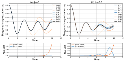
Figure 1: Time-evolution results for the one-dimensional Heisenberg model with length $L=50$, obtained using the Pauli propagation and TDVP methods, respectively. The orange lines denote TDVP results for different maximum bond dimensions $D$, and the blue lines denote Pauli propagation results for different $K$ values. For one representative curve, we also compare the absolute deviations from the exact results. (a) For $J_{x}=J_{y}=1$ and $J_{z}=0$, Pauli propagation attains accurate results at tiny cost, whereas for TDVP the error accumulates rapidly once the entanglement entropy exceeds the MPS capacity. (b) For $J_{z}\neq 0$, TDVP behaves similarly, while the computational cost of Pauli propagation is strongly affected by $J_{z}$ and becomes comparable to TDVP.

As shown in Fig. 1(a), when $J_{z}=0$, the Pauli propagation method attains accurate results with a very small Top-$K$ budget of $2^{12}$. In contrast, for TDVP, once $t>8$ the entanglement entropy exceeds the MPS capacity and the error accumulates rapidly. As shown in Fig. 1(b), when $J_{z}\neq 0$, TDVP behaves similarly, whereas the computational cost of Pauli propagation is strongly affected by $J_{z}$ and the accuracy becomes comparable to TDVP. Note that an MPS with bond dimension $D=80$ and Pauli propagation with $K=2^{19}$ have comparable numbers of free real parameters (about 730,000 for MPS and 512,000 for Pauli propagation).

Additionally, the exact reference results in the figure are obtained using TDVP without any bond dimension truncation. Therefore, we disregard Trotter errors and focus on comparing different representations as well as the impact of the corresponding truncation strategies.

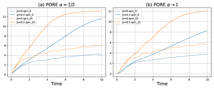
Figure 2: $\alpha=1/2$ and $\alpha\rightarrow 1$(Shannon) OSE over time. Where the blue line denotes the entropy of the Pauli Z operator with time evolution on the open boundary, and the orange line denotes the entropy corresponding to the Pauli Z operator with time evolution at the center of the one-dimensional chain.

In Fig. 2, we plot the OSE at $\alpha=1/2$ and $\alpha\rightarrow 1$ (Shannon) over time. In both cases, the entropy increases with time, indicating that the operator becomes more and more complex with time evolution. Moreover, for a fixed time the entropy increases with $J_{z}$, reflecting greater operator complexity as $J_{z}$ increases.

As shown in Theorem 1, once the target tolerance $\varepsilon$ is given, the required value of $K$ is entirely determined by the OSE. As an example, consider the propagation of the Pauli Z operator at the chain center: the maximum value of $\mathcal{S}^{\frac{1}{2}}(O)$ is $6.08$ for $J_{z}=0$ and $13.18$ for $J_{z}=0.5$, respectively. While setting $\varepsilon=0.001$, a sufficient condition to meet this error is $K>8.7\times 10^{8}$ for $J_{z}=0$ and $K>1.1\times 10^{12}$ for $J_{z}=0.5$. Note that this bound is a loose theoretical estimate. In practice, our numerical results in Fig. 1(a) show that it achieves accurate results once $K>4\times 10^{4}$. Additionally, we indeed numerically observed a higher cost when entropy is larger in the case of $J_{z}\neq 0$.

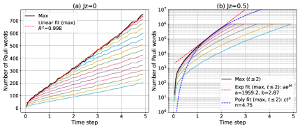
Figure 3: Growth behavior of Pauli words over time for different $J_{z}$ values.

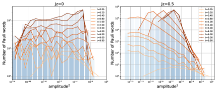
Figure 4: Distribution of the squared Pauli coefficients as a function of time for different values of $J_{z}$.

In Fig. 3, we plot the growth behavior of Pauli operators with non-zero coefficients over time for different $J_{z}$ values. For $J_{z}=0$, the number of Pauli coefficients grows almost exclusively linearly in time. This linear scaling implies that efficiently exact simulation of the dynamic evolution using Pauli propagation method is possible, which is consistent with our theoretical analysis.

While for $J_{z}=0.5$, the growth accelerates significantly and shows a quadratic growth trend. In Fig. 4, we plot the distribution of the squared Pauli coefficients as a function of time for different values of $J_{z}$. We can see that the distribution of the squared Pauli coefficients becomes more dispersed with time, and the dispersion becomes more significant with the increase of $J_{z}$.

V Conclusions and Discussions

In this work, we have introduced and analyzed a Pauli propagation framework for simulating the real-time evolution of local observables in quantum spin systems. The core of our method is to efficiently back-propagate the target observable through elementary Pauli evolutions with a computationally feasible Top-$K$ truncation strategy that retains only the most significant Pauli coefficients at each evolution step.

For analytical error bound, we have derived rigorous a priori bounds that explicitly link the truncation accuracy to OSE. We derived the relationship between truncation threshold $K$ and the OSE, establishing that higher OSE values necessitate larger $K$ for accurate simulations. Theorem 1 provides a prescription for choosing the truncation threshold K to achieve a desired accuracy $\varepsilon$, establishing that the simulation cost is governed by the intrinsic operator complexity rather than the entanglement of the quantum state. Our approach circumvents the entanglement barriers that challenge state-based tensor network methods.

We further demonstrated the compressibility of Heisenberg-evolved operators through an analytical study of the 1D XY model ($J_{z}=0$). We showed that the number of non-zero Pauli coefficients generated from a local operator grows only quadratically with the number of Trotter steps, $\mathcal{O}(s^{2})$. This analytical result demonstrated a specific example of the advantage of our method in simulating local observables in models with lower operator complexity, where the computational complexity remains manageable even at late times.

Numerical benchmarks on the one-dimensional Heisenberg model confirm the theoretical results. In the free regimes ($J_{z}=0$), the method attains high accuracy with a small Top-$K$ threshold $K=2^{12}$ and significantly outperforms TDVP, which fails at longer times due to entanglement growth. In interacting regimes ($J_{z}\neq 0$), the method remains competitive with TDVP, though the required K increases, reflecting the higher OSE values observed in Fig. 2. The growth in the number of Pauli terms Fig. 3 and the evolution of the coefficient distribution Fig. 4 further corroborate the connection between computational cost and operator complexity as measured by the OSE.

While our method offers a powerful alternative for simulating local observables, its performance is not universally efficient. The computational cost increases with the OSE, which is typically higher for strongly interacting systems or for non-local observables. Future work will explore the integration of higher-order Trotter formulas to better separate truncation errors from Trotter errors, and the combination of this framework with techniques like operator-space time-evolving decimation and MPO compression. Extensions to open quantum systems, higher dimensions, and the development of stochastic variants based on importance sampling of Pauli paths are promising directions.

In summary, the Pauli propagation method establishes an observable-centric alternative to state-based simulators for quantum dynamics simulation. It is particularly advantageous for problems where the relevant observables have low operator complexity, such as in transport studies or the calculation of out-of-time-order correlators, offering a scalable pathway in regimes where the growth of state entanglement limits traditional methods.

Appendix A Computational Cost

We analyze the computational complexity of Algorithm 1 in terms of the number of qubits $n$, number of Trotter steps $N$, number of Pauli terms in the Hamiltonian $N_{H}$, and the Top-$K$ budget $K$.

The computational cost comprises three main components:

Pauli conjugation

For a term $P_{i}$ in Hamiltonian and $n$-qubit Pauli $P_{\alpha}$ in evolved observable, Eq. (6) yields:

$$\Big(e^{-iw_{i}P_{i}\,\tau}\Big)^{\dagger}P_{\alpha}\Big(e^{-iw_{i}P_{i}\,\tau}\Big)$$ (18)

$$=$$

To implement this, we represent each Pauli operator $P_{\alpha}$ by a pair of binary strings $(\mathbf{x},\mathbf{z})\in\{0,1\}^{2n}$, where the $j$-th bits of $\mathbf{x}$ and $\mathbf{z}$ indicate whether $X$ or $Z$ acts on qubit $j$, respectively, with $Y$ represented by both bits being $1$. The (anti)commutation relation between $P_{i}$ and $P_{\alpha}$ can be determined by calculating the symplectic inner product of their binary representations with $\order{n}$ time complexity. If they commute, the conjugation leaves $P_{\alpha}$ unchanged. If they anticommute, we compute the product $P_{i}P_{\alpha}$ by performing bitwise XOR operations on their binary strings, which also takes $\order{n}$ time. Then, we update the coefficients according to the formula above, which takes $\order{1}$ time. Therefore a single conjugation costs $T_{\mathrm{conj}}(n)=\order{n}$.

Per Hamiltonian term within one time step.

For any time slice $s$ and a Hamiltonian term $P_{i}$, we need to compute the conjugation by $\Big(e^{-iw_{i}P_{i}\,\tau}\Big)^{\dagger}$ applied to all terms in the truncated observable $\widehat{O}_{s-1}$, followed by coefficient aggregation and Top-$K$ selection. Because the truncated observable $\widehat{O}_{s-1}$ contains at most $K$ operators, conjugating each of these $K$ terms produces at most two output terms per input (one if commuting; a two-term linear combination if anticommuting), resulting in at most $2K$ candidate terms. We aggregate coefficients of identical Pauli words using a hash table keyed by $(\mathbf{x},\mathbf{z})$. Finally, we select the Top-$K$ terms by magnitude from the at most $2K$ candidates. The costs of these three components are:

• Conjugations: There are at most $K$ calls to the Pauli conjugation procedure, costing $\order{K\,T_{\mathrm{conj}}(n)}=\order{Kn}$.

• Coefficient aggregation: There are at most $2K$ hash insert/update operations, the cost is expected to be $\order{K}$.

• Top-$K$ selection (Approximate Top-$K$): In our implementation, we don’t need to select the exact Top-$K$ terms; an approximate Top-$K$ suffices. To achieve this, we use a bucket-based selection method: First, we preset $B$ magnitude buckets covering the range of possible coefficient magnitudes. For example, if the maximum coefficient magnitude is $1$, we can set bucket as $[1/2,1),[1/4,1/2),[1/8,1/4),\ldots,[1/2^{B},1/2^{B-1})$, for a Pauli coefficient $c$, it falls into bucket $b$ if $2^{-(b+1)}\leq|c|<2^{-b}$. For each candidate coefficient, we place it into the corresponding bucket in $\order{1}$ time, giving $\order{K}$ time for all $\leq 2K$ candidates. The next step is to scan the buckets from high to low magnitude until collecting at least $K$ items, and return them as the approximate Top-$K$ set, which costs $\order{1}$ time with fixed $B$. Overall, the approximate Top-$K$ selection costs $\order{K}$ time.

Hence, for one $P_{i}$ in a time step, the total cost is $T_{\text{one }P_{i}}(n,K)=\order{Kn}$.

Per time step and total evolution.

Each time step processes all $N_{H}$ Hamiltonian terms in sequence, so the cost per time step is:

$$T_{\mathrm{step}}(n,K,N_{H})=\order{N_{H}\,K\,n}.$$ (19)

Over $N$ steps, the overall cost of the back-propagation evolution is:

$$T_{\mathrm{backprop}}=\order{N\,N_{H}\,K\,n}.$$ (20)

Final rescaling and expectation evaluation.

After completing the back-propagation, we need to rescale the truncated observable $\widehat{O}_{0}$ to match the Hilbert-Schmidt norm of the original observable $\widehat{O}_{0}\rightarrow\widehat{O}_{0}\cdot\frac{\norm{O}_{2}}{\norm{\widehat{O}_{0}}_{2}}$, and then evaluate the expectation value $\langle\widehat{O}\rangle_{\rho(t)}=\tr{\widehat{O}_{0}\rho(0)}$. To compute $\frac{\norm{O}_{2}}{\norm{\widehat{O}_{0}}_{2}}$, assuming the norm of $O$ is pre-computed, we use the fact that the Pauli operators form an orthonormal basis under the Hilbert-Schmidt inner product:

$$\norm{\widehat{O}_{0}}_{2}^{2}=\tr{\widehat{O}_{0}^{\dagger}\widehat{O}_{0}}=\tr{\left(\sum_{\alpha=1}^{K}c_{\alpha}P_{\alpha}\right)^{\dagger}\left(\sum_{\beta=1}^{K}c_{\beta}P_{\beta}\right)}=2^{n}\sum_{\alpha=1}^{K}c_{\alpha}^{2}.$$ (21)

Thus, the cost of rescaling is $\order{K}$ to obtain $\sum_{\alpha=1}^{K}c_{\alpha}^{2}$. Next, we evaluate the expectation value $\langle\widehat{O}\rangle_{\rho(t)}$. For a product state $\rho(0)=\otimes_{j=1}^{n}\rho_{j}$, and an expansion $\widehat{O}_{0}=\sum_{\alpha=1}^{K}c_{\alpha}P_{\alpha}$ with $P_{\alpha}=\bigotimes_{j=1}^{n}P_{\alpha,j}$, linearity yields

$$\langle\widehat{O}\rangle_{\rho(t)} =\tr{\widehat{O}_{0}\,\rho(0)}$$ (22)

$$=\sum_{\alpha=1}^{K}c_{\alpha}\,\tr{P_{\alpha}\,\rho(0)}$$

$$=\sum_{\alpha=1}^{K}c_{\alpha}\prod_{j=1}^{n}\tr{P_{\alpha,j}\,\rho_{j}}.$$

Each term $\tr{P_{\alpha,j}\,\rho_{j}}$ can be computed in $\order{1}$ time, so the total cost for evaluating the expectation value is $\order{K\,n}$.

Therefore, the total computational cost of Algorithm 1 is:

$$T_{\mathrm{total}}(n,K,N_{H},N)=\order{N\,N_{H}\,K\,n+K\,n}=\order{N\,N_{H}\,K\,n}.$$ (23)

Appendix B Proof of Lemma 1

Proof.

The proof is straightforward by using the properties of the OSE.

1. We consider the tensor product of two observables $O=O_{1}\otimes O_{2}$, and denote the Pauli coefficients of $O$, $O_{1}$ and $O_{2}$ as $\bm{c}$, $\bm{c}_{1}$ and $\bm{c}_{2}$ respectively. For $P=P_{1}\otimes P_{2}$, we have $c_{P}=c_{P_{1}}c_{P_{2}}$ for $P_{1}\in\{I,X,Y,Z\}^{\otimes n_{1}}$ and $P_{2}\in\{I,X,Y,Z\}^{\otimes n_{2}}$. Therefore, we have:

   $$\norm{\bm{c^{2}}}^{\alpha}_{\alpha} =\sum_{P_{1}\in\{I,X,Y,Z\}^{\otimes n_{1}}}\sum_{P_{2}\in\{I,X,Y,Z\}^{\otimes n_{2}}}c_{P_{1}\otimes P_{2}}^{2\alpha}$$ (24)

   $$=\sum_{P_{1}\in\{I,X,Y,Z\}^{\otimes n_{1}}}c_{P_{1}}^{2\alpha}\sum_{P_{2}\in\{I,X,Y,Z\}^{\otimes n_{2}}}c_{P_{2}}^{2\alpha}$$

   $$=\norm{\bm{c^{2}}_{1}}^{\alpha}_{\alpha}\norm{\bm{c^{2}}_{2}}^{\alpha}_{\alpha}.$$

   Taking into the entropy definition, we have:

   $$\mathcal{S}^{\alpha}(O)=\mathcal{S}^{\alpha}(O_{1})+\mathcal{S}^{\alpha}(O_{2}).$$ (25)

2. Consider the conjugation of $O$ by a Clifford circuit $U$, we denote the Pauli coefficients of $UOU^{\dagger}$ as $\bm{c}^{\prime}$. For $Q=U^{\dagger}PU$ with $P\in\{I,X,Y,Z\}^{\otimes n}$, by the property of the Clifford circuit, we have $Q\in\{I,X,Y,Z\}^{\otimes n}$ and $c^{\prime}_{Q}=c_{P}$. Therefore, we have:

   $$\norm{\bm{c^{\prime}}^{2}}_{\alpha}=\norm{\bm{c^{2}}}_{\alpha}.$$ (26)

   Taking into the entropy definition, we have:

   $$\mathcal{S}^{\alpha}(UOU^{\dagger})=\mathcal{S}^{\alpha}(O).$$ (27)

3. Let $O=\sum_{i}\lambda_{i}O_{i}$ be the weighted sum of the operators $O_{i}$. The Pauli coefficients of $c_{i}(O)$ for operator $O$ is defined as $c_{i}(O)=\frac{1}{2^{n}}\tr{P_{i}O}$. We have:

   $$c_{i}(O)=\sum_{j}\lambda_{j}c_{i}(O_{j}),$$ (28)

   where $c_{i}(O_{j})=\frac{1}{2^{n}}\tr{P_{i}O_{j}}$. Since $0<\alpha<0.5$, the function $f(x)=x^{2\alpha}$ is concave, by Jensen’s inequality, we have:

   $$\left(\sum_{j}\lambda_{j}c_{i}(O_{j})\right)^{2\alpha}\geq\sum_{j}\lambda_{j}c_{i}(O_{j})^{2\alpha}.$$ (29)

   Therefore, we have:

   $$\sum_{i}\left(\sum_{j}\lambda_{j}c_{i}(O_{j})\right)^{2\alpha}\geq\sum_{i}\sum_{j}\lambda_{j}c_{i}(O_{j})^{2\alpha}.$$ (30)

   Taking into the entropy definition, we have:

   $$\mathcal{S}^{\alpha}(O)\geq\frac{1}{1-\alpha}\ln\left(\sum_{i}\sum_{j}\lambda_{j}c_{i}(O_{j})^{2\alpha}\right).$$ (31)

   By the concavity of the logarithm function, there is:

   $$\ln\left(\sum_{i}\sum_{j}\lambda_{j}c_{i}(O_{j})^{2\alpha}\right)\geq\sum_{i}\lambda_{i}\ln\left(\sum_{j}c_{i}(O_{j})^{2\alpha}\right).$$ (32)

   Therefore, we obtain $\mathcal{S}^{\alpha}(\cdot)$ is a concave function.

   $$\mathcal{S}^{\alpha}(O)\geq\sum_{i}\lambda_{i}\mathcal{S}^{\alpha}(O_{i}).$$ (33)

4. Similarly, we have:

   $$c_{i}(O)=\sum_{j}\lambda_{j}c_{i}(O_{j}),$$ (34)

   where $c_{i}(O_{j})=\frac{1}{2^{n}}\tr{P_{i}O_{j}}$.

   On the other hand, we have:

   $$\text{exp}\left(\mathcal{S}^{\alpha}(O)\right)=\left(\sum_{i}\absolutevalue{c_{i}(O)}^{2\alpha}\right)^{\frac{1}{1-\alpha}}=\left(\sum_{i}\absolutevalue{c_{i}(O)}^{q}\right)^{\frac{1}{1-\alpha}}=\norm{\bm{c}(O)}_{q}^{r},$$ (35)

   where $q=2\alpha$, $r=\frac{2\alpha}{1-\alpha}$ and $\bm{c}(O)=(c_{1}(O),c_{2}(O),\ldots,c_{4^{n}}(O))$. By Minkowski inequality, we have:

   $$\norm{\bm{c}(O)}_{q}=\norm{\sum_{j}\lambda_{j}\bm{c}(O_{j})}_{q}\leq\sum_{j}\lambda_{j}\norm{\bm{c}(O_{j})}_{q}.$$ (36)

   Therefore, we have:

   $$\text{exp}\left(\mathcal{S}^{\alpha}(O)\right)\leq\left(\sum_{j}\lambda_{j}\norm{\bm{c}(O_{j})}_{q}\right)^{r}.$$ (37)

   Since $0.5\leq\alpha<1$, we have $r\geq 2$ and the function $f(x)=x^{r}$ is convex, by Jensen’s inequality, we have:

   $$\text{exp}\left(\mathcal{S}^{\alpha}(O)\right)\leq\left(\sum_{j}\lambda_{j}\norm{\bm{c}(O_{j})}_{q}\right)^{r}\leq\sum_{j}\lambda_{j}\norm{\bm{c}(O_{j})}_{q}^{r}=\sum_{j}\lambda_{j}\text{exp}\left(\mathcal{S}^{\alpha}(O_{j})\right).$$ (38)

   Therefore, we obtain $\text{exp}\left(\mathcal{S}^{\alpha}(\cdot)\right)$ is a concave function.

∎

Appendix C Proof of Lemma 2

Proof.

Let $\varDelta(K)\coloneqq\sum_{i=K+1}^{\infty}c^{\prime 2}_{i}$. The approximated observable is given by:

$$\widehat{O}=\frac{\norm{O}_{2}}{\sqrt{2^{n}\sum_{i=1}^{K}c^{\prime 2}_{i}}}\sum_{i=1}^{K}c^{\prime}_{i}P_{i}.$$ (39)

Note that $\norm{O}_{2}^{2}=2^{n}\sum_{i=1}^{\infty}c^{\prime 2}_{i}$, we have:

$$\norm{\widehat{O}}_{2}^{2}=\norm{O}_{2}^{2}.$$ (40)

Consider the cosine similarity between $O$ and $\widehat{O}$:

$$F_{HS}(\widehat{O},O)=\frac{\tr{O^{\dagger}\widehat{O}}}{\norm{O}_{2}\norm{\widehat{O}}_{2}}=\frac{\sqrt{2^{n}\sum_{i=1}^{K}c^{\prime 2}_{i}}}{\norm{\widehat{O}}_{2}}.$$ (41)

The Hilbert-Schmidt distance can be related to the cosine similarity as:

$$\norm{O-\widehat{O}}_{2}^{2} =\norm{O}_{2}^{2}+\norm{\widehat{O}}_{2}^{2}-2\norm{O}_{2}\norm{\widehat{O}}_{2}F_{HS}(\widehat{O},O)$$ (42)

$$=2\norm{O}_{2}^{2}(1-F_{HS}(\widehat{O},O)).$$

On the other hand, by $2^{n}\sum_{i=1}^{K}c^{\prime 2}_{i}=\norm{O}_{2}^{2}-2^{n}\varDelta(K)$, we have:

$$1-F_{HS}(\widehat{O},O) =\frac{\norm{O}_{2}-\sqrt{\norm{O}^{2}_{2}-2^{n}\varDelta(K)}}{\norm{O}_{2}}$$ (43)

$$=\frac{2^{n}\varDelta(K)}{\norm{O}_{2}\left(\norm{O}_{2}+\sqrt{\norm{O}^{2}_{2}-2^{n}\varDelta(K)}\right)}$$

$$\leq\frac{2^{n}\varDelta(K)}{\norm{O}^{2}_{2}}.$$

Therefore, the derivation can be upper bound by:

$$\norm{O-\widehat{O}}_{Pauli,2}=\frac{1}{\sqrt{2^{n}}}\norm{O-\widehat{O}}_{2}=\sqrt{2\varDelta(K)}.$$ (44)

∎

Appendix D Proof of Thm. 1

Proof.

First, the $\{c^{\prime 2}_{i}\}_{i=1}^{\infty}$ is a nonincreasingly sequence, we have:

$$\absolutevalue{c^{\prime 2}_{i}}^{\alpha}\leq\frac{1}{i}\sum_{j=1}^{i}\absolutevalue{c^{\prime 2}_{j}}^{\alpha}\leq\frac{1}{i}\sum_{j=1}^{\infty}\absolutevalue{c^{\prime 2}_{j}}^{\alpha}.$$ (45)

Therefore, we have:

$$\varDelta(K)=\sum_{i=K+1}^{\infty}c^{\prime 2}_{i}\leq\sum_{i=K+1}^{\infty}\left(\frac{1}{i}\sum_{j=1}^{\infty}\absolutevalue{c^{\prime 2}_{j}}^{\alpha}\right)^{\frac{1}{\alpha}}=\left(\sum_{i=K+1}^{\infty}i^{-\frac{1}{\alpha}}\right)\left(\sum_{j=1}^{\infty}\absolutevalue{c^{\prime 2}_{j}}^{\alpha}\right)^{\frac{1}{\alpha}}.$$ (46)

On the other hand, there is :

$$\sum_{i=K+1}^{\infty}i^{-\frac{1}{\alpha}}\leq\int_{K}^{\infty}x^{-\frac{1}{\alpha}}\mathrm{d}x=\frac{\alpha}{1-\alpha}K^{\frac{\alpha-1}{\alpha}}.$$ (47)

Therefore, we have:

$$\ln{\varDelta(K)}\leq\ln{\frac{\alpha}{1-\alpha}}+\frac{\alpha-1}{\alpha}\ln{K}+\frac{1}{\alpha}\ln{\left(\sum_{j=1}^{\infty}\absolutevalue{c^{\prime 2}_{j}}^{\alpha}\right)}=\frac{1-\alpha}{\alpha}\left(\mathcal{S}^{\alpha}(O)-\ln{K}\right)+\ln{\frac{\alpha}{1-\alpha}}.$$ (48)

This completes the proof of the theorem.

By Lemma 2, we have:

$$\norm{O-\widehat{O}}_{Pauli,2}\leq\sqrt{2\varDelta(K)}\leq\sqrt{2\frac{\alpha}{1-\alpha}}\text{exp}\left(\frac{1-\alpha}{2\alpha}\left(\mathcal{S}^{\alpha}(O)-\ln{K}\right)\right).$$ (49)

To guarantee that $\norm{O-\widehat{O}}_{Pauli,2}\leq\varepsilon$, it is sufficient to choose $K$ such that:

$$K\geq\text{exp}\left(\mathcal{S}^{\alpha}(O)\right)\left(\frac{2\alpha}{(1-\alpha)\varepsilon^{2}}\right)^{\frac{\alpha}{1-\alpha}}.$$ (50)

∎

Appendix E Proof of Thm. 2

Proof.

The Trotterized evolution employs the following gates:

$$U_{j,j+1}(\theta_{1})=\text{exp}\left(i\theta X_{j}X_{j+1}\right),$$ (51)

and

$$V_{j,j+1}(\theta_{2})=\text{exp}\left(i\theta Y_{j}Y_{j+1}\right),$$ (52)

where $\theta_{1}=-J_{X}\tau$ and $\theta_{2}=-J_{Y}\tau$, respectively.

Define the operators $J_{i,j}=X_{i}Z_{i+1}\ldots Z_{j-1}Y_{j}$, $H_{i,j}=Y_{i}Z_{i+1}\ldots Z_{j-1}X_{j}$, $K_{i,j}=X_{i}Z_{i+1}\ldots Z_{j-1}X_{j}$ and $L_{i,j}=Y_{i}Z_{i+1}\ldots Z_{j-1}Y_{j}$. The subspace:

$${span}\left\{Z_{l},J_{l,m},H_{l,m},K_{l,m},L_{l,m}\right\}$$ (53)

is invariant under the conjugation by $U_{j,j+1}(\theta)$ and $V_{j,j+1}(\theta)$.

For example, conjugating $Z_{l}$ by $U_{j,j+1}(\theta_{1})$, we have:

$$U_{j,j+1}(\theta_{1})^{\dagger}Z_{l}U_{j,j+1}(\theta_{1})$$ (54)

$$=$$

which confirms the claimed invariance.

For other operators in the algebra, the conjugation action can be verified similarly.

On the other hand, after $s$-step Trotterization, the light-cone of $Z_{l}$ is contained in the interval $[l-s,l+s]$. Consequently, the number of non-zero Pauli coefficients in the evolved operator $Z_{l}$ is upper bounded by:

$$\binom{2s}{1}+4\binom{2s}{2}=2s+4s(2s-1)=\order{s^{2}},$$ (55)

where $\binom{2s}{1}$ counts the number of $Z_{i}$ terms, and $4\binom{2s}{2}$ counts the number of $J_{i,j},H_{i,j},K_{i,j},L_{i,j}$ terms.

∎

Appendix F Weight Truncation

For weight truncation, previous works [43] have established error bounds under structural assumptions such as local scrambling. We assume the state $\rho$ is sampled from a local-scrambling ensemble, i.e $\rho=V\outerproduct{0}{0}^{\otimes n}V^{\dagger}$ with $V$ sampled from a local-scrambling ensemble. Then, the expectation error is bounded by:

Theorem 3.

Let $O=\sum_{P\in\{I,X,Y,Z\}^{\otimes n}}c_{P}P$ be an observable and $\widehat{O}$ be the approximated observable obtained by weight truncation with threshold $M$ and normalized:

$$\widehat{O}=\frac{\norm{O}_{2}}{\sqrt{2^{n}\sum_{wt(P)<M}c_{P}^{2}}}\sum_{wt(P)<M}c_{P}P,$$ (56)

where $wt(P)$ is the Hamming weight of the Pauli word $P$, i.e., the number of non-identity Paulis in $P$. Then for a state $\rho$ sampled from a local-scrambling ensemble, we have:

$$\mathbb{E}_{\rho}\absolutevalue{\langle\widehat{O}\rangle_{\rho}-\langle O\rangle_{\rho}}^{2}\leq\left(\frac{2}{3}\right)^{M}\norm{O}_{Pauli,2}^{2}+\sum_{wt(P)\geq M}c_{P}^{2},$$ (57)

where $\norm{O}_{Pauli,2}=\sqrt{\sum_{P}c^{2}_{P}}$ is normalized Hilbert-Schmidt norm.

This result is similar to that in Ref. [43], except that there is a normalization procedure after truncation in our method.

In our numerical experiments, we observe that, in 1D heisenberg chain, the weight truncation strategy is nonessential, since under the Top-$K$ truncation only lower weights usually survive.

As shown in Fig. 5, we analyze the distribution of the Pauli words coefficients in terms of their Hamming weight. We can see that the distribution of the Pauli words coefficients becomes more dispersed with time, and the dispersion becomes more significant with the increase of $J_{z}$. This indicates that the strategy of deactivate weight truncation is effective. Moreover, we could observe that as time evolves, the operator becomes more complex and involves more qubits, and the increase of $J_{z}$ further enhances this effect.

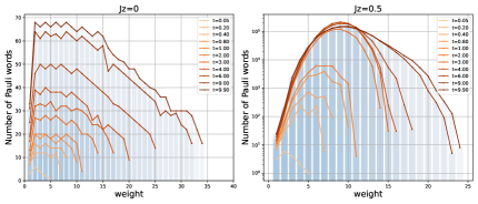
Figure 5: Pauli weight distribution of the Pauli words coefficients as a function of time for different values of $J_{z}$.

F.1 Proof of Theorem 3

Proof.

The proof is similar to that in Ref. [43], except that there is a normalization procedure after truncation in our method. By $\rho=V\outerproduct{0}{0}^{\otimes n}V^{\dagger}$ with $V$ sampled from a local-scrambling ensemble, we have:

$$\mathbb{E}_{\rho}\absolutevalue{\langle\widehat{O}\rangle_{\rho}-\langle O\rangle_{\rho}}^{2}=\mathbb{E}_{V}\absolutevalue{\tr{V^{\dagger}(\widehat{O}-O)V\outerproduct{0}{0}^{\otimes n}}}^{2}.$$ (58)

The difference between the approximated observable and the original observable is given by:

$$\widehat{O}-O=$$ (59)

$$\left(\frac{\norm{O}_{2}}{\sqrt{2^{n}\sum_{wt(P)<M}c_{P}^{2}}}-1\right)\left(\sum_{wt(P)<M}c_{P}P\right)$$

$$-\left(\sum_{wt(P)\geq M}c_{P}P\right).$$

Using the property of local-scrambling ensemble (Lemma 7 in Ref. [43]), we have:

$$\mathbb{E}_{V}\tr{V^{\dagger}PV\outerproduct{0}{0}^{\otimes n}}\tr{V^{\dagger}QV\outerproduct{0}{0}^{\otimes n}}$$ (60)

$$=$$

where the summation of $W$ is over all Pauli words with same support as $P$, i.e., $\mathrm{supp}(W)=\mathrm{supp}(P)$ for $W\in\{I,X,Y,Z\}^{\otimes n}$.

On the other hand, by Lemma 10 in Ref. [43], there is:

$$\mathbb{E}_{V}\tr{V^{\dagger}WV\outerproduct{0}{0}^{\otimes n}}^{2}\leq\left(\frac{2}{3}\right)^{wt(W)}.$$ (61)

Combining the above equations, we have:

$$\mathbb{E}_{V}\absolutevalue{\tr{V^{\dagger}(\widehat{O}-O)V\outerproduct{0}{0}^{\otimes n}}}^{2}$$ (62)

$$\leq\left(\frac{\norm{O}_{2}}{\sqrt{2^{n}\sum_{wt(P)<M}c_{P}^{2}}}-1\right)^{2}\left(\sum_{wt(P)<M}c_{P}^{2}\right)$$

$$+\left(\sum_{wt(P)\geq M}\left(\frac{2}{3}\right)^{wt(P)}c_{P}^{2}\right)$$

Using $\norm{O}_{2}^{2}=2^{n}\sum_{P}c_{P}^{2}$, we have:

$$\left(\frac{\norm{O}_{2}}{\sqrt{2^{n}\sum_{wt(P)<M}c_{P}^{2}}}-1\right)^{2}$$ (63)

$$=\left(\frac{\sqrt{2^{n}\sum_{P}c_{P}^{2}}}{\sqrt{2^{n}\sum_{wt(P)<M}c_{P}^{2}}}-1\right)^{2}$$

$$\leq\frac{\sum_{wt(P)\geq M}c_{P}^{2}}{\sum_{wt(P)<M}c_{P}^{2}}.$$

Therefore, we have:

$$\mathbb{E}_{\rho}\absolutevalue{\langle\widehat{O}\rangle_{\rho}-\langle O\rangle_{\rho}}^{2}\leq\left(\frac{2}{3}\right)^{M}\norm{O}_{Pauli,2}^{2}+\sum_{wt(P)\geq M}c_{P}^{2}.$$ (64)

∎