Deprojection of Galaxy Cluster X-ray, Sunyaev-Zel’dovich Temperature Decrement and Weak Lensing Mass Maps

Abstract

A general method of deprojecting two-dimensional images to reconstruct the three dimensional structure of the projected object – specifically X-ray, Sunyaev-Zel’dovich (SZ) and gravitational lensing maps of rich clusters of galaxies – assuming axial symmetry (Zaroubi et al. (1998)), is considered. Here we test the applicability of the method for realistic, numerically simulated galaxy clusters, viewed from three orthogonal projections at four redshift outputs. We demonstrate that the assumption of axial symmetry is a good approximation for the 3D structure in this ensemble of galaxy clusters. Applying the method, we demonstrate that a unique determination of the cluster inclination angle is possible from comparison between the SZ and X-ray images and, independently, between SZ and surface density maps. Moreover, the results from these comparisons are found to be consistent with each other and with the full 3D structure inclination angle determination. The radial dark matter and gas density profiles as calculated from the actual and reconstructed 3D distributions show a very good agreement. The method is also shown to provide a direct determination of the baryon fraction in clusters, independent of the cluster inclination angle.

1 Introduction

Recent years have witnessed significant improvements in the quality and quantity of data from clusters of galaxies in all wavebands, from the X-ray, through optical, to radio wavelengths. Together with advances in the theoretical modeling of the physical processes in clusters, these improvements call for new and more accurate methods of data analysis and comparison with various theoretical predictions.

In particular, uncovering the 3D structure of clusters is of great interest as it plays an important role in the determination of the Hubble constant from X-ray and SZ measurements (see Appendix), cluster mass and baryon fraction determination, and the underlying galaxy orbit structure. In order to reconstruct the 3D geometry of clusters researchers normally apply the spherical symmetry assumption, either within a parametric (e.g., Cavaliere & Fusco-Femiano 1976) or non-parametric (Fabian et al. 1981; and more recently Yushikawa & Suto 1999) framework. Although this simplifying assumption is very useful for many problems, it can lead to significant biases in others, e.g., the Hubble constant determination (e.g., Fabricant et al 1984).

Recently, a few studies have developed methods to take advantage of the full two dimensional information retained in the cluster images and extend the modeling of the underlying three dimensional structure to have a more general, aspherical distribution (e.g., Zaroubi et al. 1998; Reblinsky & Bartelmann 1999). In particular, Zaroubi et al. (1998; hereafter referred to as paper I) presented a model-independent method of image deprojection for probing the 3D structure in clusters of galaxies, assuming only that the underlying 3D structure has axial symmetry. The original testing of this method demonstrated that given images of the cluster in the X-ray, radio and a map of the projected total mass distribution, one could uniquely determine the inclination angle of the system symmetry axis, and determine the underlying 3D structure in the gas and dark matter (see also Grego et al.  2000). They studied the stability of the inversion method in the context of a specific analytical gas density profile: an axially symmetric, elliptical isothermal model; which is an extension of the widely used isothermal sphere model.

A few questions arise from the study in paper I: 1) Is the fundamental assumption of axial symmetry valid for real galaxy clusters? 2) Does substructure and dynamical evolution in galaxy clusters (as predicted to be abundant by hierarchical structure formation models) permit a robust, unique and stable numerical application of the method? 3) Can the cluster symmetry axis inclination angle be uniquely determined for more complex cluster gas/mass density distributions? 4) With realistic expected resolution and signal-to-noise from current observations, can the method be applied?

To probe these questions, we have performed a study of the inversion algorithm on a set of numerically simulated galaxy clusters. The goal is to test the axisymmetric deprojection algorithm, using as input a representative realization of the cluster population. We would like to emphasize at this stage that testing the applicability of the technique to current data sets is beyond the scope of the current paper. The method should be applied to each data set while taking into account its unique specifications, e.g., resolution, scanning strategy, data acquisition domain (UV plane vs. real space), etc. We intend indeed to tackle these issues for specific data sets in a forthcoming paper.

The outline of this study is as follows. In §2 the deprojection method is briefly reviewed, and we develop a new feature of the method that allows an inclination angle-independent determination of the baryon fraction in clusters. In §3, we briefly describe the input cluster simulations. In §4, we show in detail the results for a single, prototype simulated cluster. In §5, we apply the method to the full cluster simulation output. The paper is concluded with a discussion (§6).

2 The Deprojection Method

The method for deprojection is described elsewhere (Zaroubi et al. (1998)). Briefly, we deproject cluster images as follows. We adopt the convention that bold-face symbols denote 3D quantities (e.g., ${\bf k}=(k_{x},k_{y},k_{z})$). Let the observer’s coordinate system be defined with the Cartesian axes $(x^{\prime},y^{\prime},z^{\prime})$, with the $z^{\prime}$ axis aligned with the line of sight. Denote the (cluster) source function coordinate system by the axes $(x,y,z)$ where the $z$-axis is the cluster symmetry axis, forming an angle $\theta_{i}$ with respect to the line of sight (see diagram shown in Figure 1). Let $I(x^{\prime},y^{\prime})=\int\lambda^{\prime}({\bf x^{\prime}})dz^{\prime}$ denote a projected quantity (image) of the source function $\lambda$. The 3D Fourier transform (FT) of the source function is related to the image Fourier transform by

$$\lambda_{\bf k^{\prime}}^{\prime}(k_{x}^{\prime},k_{y}^{\prime},0) = \int e^{[-i(k^{\prime}_{x}x^{\prime}+k^{\prime}_{y}y^{\prime})]}I(x^{\prime},y^{\prime})\,{\rm d}x^{\prime}\,{\rm d}y^{\prime}$$ (1)

$$= I_{k^{\prime}}(k_{x}^{\prime},k_{y}^{\prime}).$$

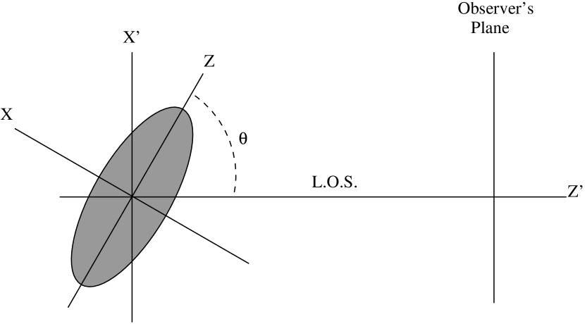
Figure 1: A diagram showing the coordinate systems used in the paper. $(x^{\prime},y^{\prime},z^{\prime})$ denote the the observers coordinates with $z^{\prime}$ aligned with the line of sight. $(x,y,z)$ denote the cluster source function coordinates with $z$-axis is the cluster symmetry axis.

The expression relating the FT of the source function in the observer and cluster rest frames is obtained simple by coordinate rotation, so that

$$\lambda_{k^{\prime}}^{\prime}({\bf k^{\prime}}) = \lambda_{k}\biggl{(}\sqrt{(-k_{z}^{\prime}\sin\theta_{i}+k_{x}^{\prime}\cos\theta_{i})^{2}+k_{y}^{\prime\,2}},k_{z}^{\prime}\cos\theta_{i}+k_{x}^{\prime}\sin\theta_{i}\biggr{)}$$ (2)

$$= \lambda_{k}(k,k_{z}).$$

where the last equality again holds due to axial symmetry. Inverse transforming, we find the desired expression for the source function in real space

$$\lambda^{\rm deproj}(r,z)={\frac{1}{(2\pi)^{2}}}\int k\,dk\,dk_{z}\,e^{ik_{z}z}J_{0}(k\,r)\,I_{k^{\prime}}\biggl{(}\frac{k_{z}}{\sin\theta_{i}},\sqrt{k^{2}-k^{2}_{z}\cot^{2}\theta_{i}}\biggr{)}.$$ (3)

The implementation of this method is straightforward, assuming for the moment that the inclination angle is known. The image FT is evaluated at wavevectors

$$k_{x}^{\prime}=k_{z}/\sin\theta_{i}\;\;\;{\rm and}\;\;\;k_{y}^{\prime}=\sqrt{k^{2}-k_{z}^{2}\cot\theta_{i}^{2}}$$ (4)

and the inverse transform applied.

For wavevectors $k<|k_{z}|\,\cot\theta_{i}$, the argument of the image FT becomes imaginary defining a cone in k-space known as the “cone of ignorance” (hereafter COI).

An interesting property of equation (3) is that the k-space information in the $k_{z}=0$ plane is fully known and independent of the cluster inclination angle. It is, therefore, straightforward to show, by integrating over Eq. 2 with respect to $z$, that the projection over the $x^{\prime}$-direction is related to the symmetry axis integrated density,

$$\rho^{z}(r)\equiv\int\lambda(r,z)dz={\frac{1}{2\pi}}\int k\,dkJ_{0}(k\,r)\,I_{k^{\prime}}(0,k),$$

where $I_{k^{\prime}}(0,k)$ is FT of $\int I(x^{\prime},y^{\prime})dx^{\prime}$. We can also define the z-projected cluster ‘mass’, $M^{z}(r)=\pi\int\rho^{z}(r)\,r\,dr$.

This relation is especially useful in the case of isothermal clusters, where the SZ map is proportional to the projected electron number density, hence to the projected gas density, and the surface density map is proportional to the projected total mass density. Therefore equation (2) provides an angle independent estimate of $\Omega_{b}/\Omega$, and enables evaluation of the ratio $\rho^{z}_{\rm gas}/\rho^{z}_{DM}$ and $M^{z}_{\rm gas}/M^{z}_{DM}$ as a function of the distance from the symmetry axis. Note also that since the gas and total mass distributions for an isothermal cluster are roughly proportional to each other in most of the volume (Ettori & Fabian (1999)), except the inner most region, this comparison is almost Hubble constant independent.

3 The Cluster Sample

To test the validity of the deprojection method, we employed a set of outputs from a gas dynamic simulation of the formation of an X-ray cluster. The simulation is Evrard’s contribution to the Santa Barbara cluster comparison project (Frenk et al. (1998)). Details of the simulation are provided elsewhere (Frenk et al. (1998)), but we very briefly outline the data set here:

The underlying structure formation model was CDM, with the G3 transfer function fit of Bardeen et al. (1986) at $z=20$. The simulation was performed in a flat universe, the initial fluctuation spectrum was given a shape parameter of $\Gamma=0.25$ and normalized such that the present day rms mass fluctuations in a spherical top-hat of radius $16\,h_{0.5}^{-1}{\rm Mpc}$ is $\sigma_{8}=0.65$. The cosmological parameters were assigned with as $H_{0}=50\;{\rm km/s/Mpc}$, $\Omega=1$, and a contribution from the baryons of $\Omega_{b}=0.1$.

The initial conditions for the simulation were generated with a constrained Gaussian random field (Hoffman & Ribak (1991)), and galaxy clusters identified with $3\sigma$ peaks of the field smoothed with a Gaussian filter of scale $10\,h_{0.5}^{-1}{\rm Mpc}$, and centered in a cubic region of side $64\,h_{0.5}^{-1}{\rm Mpc}$.

The evolution of the gas was followed using the Smoothed Particle Hydrodynamics (SPH) technique (Evrard (1988)) to $z=0$. Final maps of the projected total mass distribution, Compton y-parameter, and simplified versions of the X-ray luminosity and X-ray emission weighted temperature were produced. The projected quantities were calculated from a $(32\,h_{0.5}^{-1}{\rm Mpc})^{3}$ cube, and computed on a $256\times 256$ grid, corresponding to a physical scale of $10\,h_{0.5}^{-1}{\rm Mpc}$ at $z=0$. In the Rayleigh-Jeans regime, the Compton y-parameter is related to the SZ decrement as $\frac{\delta T}{T}=-2y$. We have applied this conversion to the simulation output.

For the purposes of this test, we employed three orthogonal projections of a single cluster at four redshifts: $z=0,0.3,0.6,\;{\rm and}\;0.9$. This, in effect, yields a sample of 12 semi-independent clusters to study with a wide range of dynamical states and physical distributions of the gas and dark matter. For example, at $z=0.6$, the cluster undergoes a major merger event, and thus the outputs at that redshift permit a study of the method while the cluster is in a highly unrelaxed state.

4 Application: The Prototype Cluster

For the first part of this analysis, we concentrate on a single ‘prototype cluster’; the simulation output at $z=0$. In Figure 2, we display the logarithmically scaled mass surface density, X-ray surface brightness, SZ decrement and emission weighted temperature distributions for the three orthogonal projections of the prototype cluster. The dimensions for the surface density, temperature and SZ decrement are physical ($M_{\odot}/{\rm Mpc}^{2}$ and $K$ for the first two, while the SZ decrement is dimensionless). The X-ray surface brightness was calculated as the line of sight integral $\int\rho_{\rm gas}^{2}T^{1/2}dl$ and has dimensions $M_{\odot}^{2}K^{1/2}/{\rm Mpc}^{5}$. In this section, unless stated otherwise, the images used for deprojection are the y-projection maps of the simulated protocluster.

For the prototype cluster, the projected gas and total mass distributions are elliptical, with axis ratios $a/b\gtrsim 2:1$. In all of the projections, an infalling sublump is evident, approximately $\simeq 3\,h_{0.5}^{-1}{\rm Mpc}$ (projected distance) from the cluster center. We note that the emission weighted temperature is nearly constant over the innermost $\simeq 3\,h_{0.5}^{-1}{\rm Mpc}$, with a value of $(7.5\pm 0.5)\times 10^{7}\,K$. In what follows for this specific cluster, we treat the gas distribution as being isothermal.

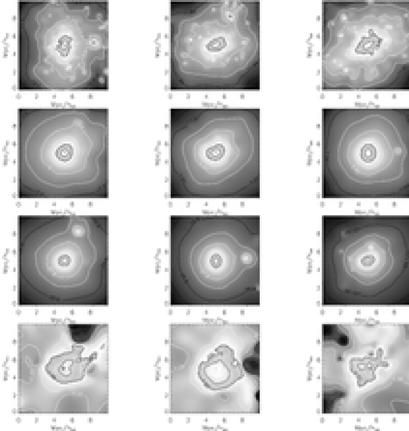
Figure 2: Left column: The x-projection for the prototype cluster. The grey scale and contours show the logarithmic intensity. Surface density (first panel; $M_{\odot}/{\rm Mpc}^{2}$), and Sunyaev-Zel’dovich decrement (second panel). X-ray surface brightness (third panel; $M_{\odot}^{2}K^{1/2}/{\rm Mpc}^{5}$), and emission weighted temperature (fourth panel; $K$). The middle and right columns show the same plots for the y- and z-projections respectively.

4.1 The Baryon Fraction

Using equation (2), we calculated the gas to total mass and density ratios for prototype cluster. The results are shown in Figure 3 for the y-projection maps. As discussed below (see §4.2.1), we do not know apriori if the cluster is prolate or oblate, and so we have calculated the ratios under both assumptions. However, this is the only unknown; no knowledge of the inclination angle is required to determine these ratios.

The value of density and mass ratios in the case of this prototype cluster is $\sim 0.1$. Under the assumption the cluster is prolate, this ratio is approximately constant at all radii, whereas in the oblate case, it rises by $\simeq 50$% towards the center. However, in both cases, at the outermost radii probed by our calculation, the density ratio becomes $\sim 0.105$ which is extremely close to the input ratio in the SPH/N-body simulation.

The density and mass ratios across the cluster, especially in relaxed clusters, are expected to have an almost constant value, with small radial dependence (Ettori & Fabian (1999)). Therefore, the greater variability shown in the density and mass ratios under the assumption of oblate cluster might be used as an indicator to that the protocluster at hand is most probably prolate. Inspection of the true 3D distribution shows that this is indeed the case. The same argument can be repeated for all the clusters we have analyzed in this paper (see Figs. 17,  18,  19, and  20).

Furthermore, the true full 3D distribution clearly shows that the gas radial density profile follows very faithfully the radial mass density profile down to the inner most $0.3{\rm Mpc}$, interior to this radius the ratio drops down due to the effect of the pressure (see Figs. 10 and 12 in Frenk et al. (1998)), which explains the drop in the gas to mass ratio at the inner most radii in the prolate case shown in the left panel of Figure 3.

Figure 3: The ratio of the z-integrated gas density and dark matter density, $\rho^{z}_{gas}/\rho^{z}_{DM}$ , as a function of r, calculated from the surface density and Sunyaev-Zel’dovich maps of the y-projection shown in the middle row of Figure 2 (solid line) and the corresponding gas to dark matter mass ratio (dashed line). The left and right panels are produced assuming a prolate and oblate cluster respectively.

4.2 The Cluster 3D Structure

To demonstrate the utility of the method for the determining the underlying 3D structure, we proceed in two ways: first, we demonstrate that a robust and stable determination of the inclination angle can be achieved using the sort of information that would be available from observations (i.e., X-ray, SZ and lensing maps). Secondly, using our knowledge of the true underlying 3D structure, available since we are employing simulated clusters, we determine the accuracy with which cumulated quantities (such as gas or total mass) can be determined from this method.

We encountered several subtle features of the deprojection procedure which we describe in detail below. However, the overall procedure is, conceptually at least, straightforward: we first determine the image axis of symmetry, which is the projection of the axis of symmetry in the 3D distribution. We allow both possibilities that the cluster is either oblate or prolate, and deproject using equation (3). As the inclination angle is unknown, we deproject each image over a wide range of assumed inclination angles, searching for the angle that consistently yields the best reconstructed ratios between the Sunyaev-Zel’dovich, X-ray and the total mass deprojections, as discussed below.

4.2.1 Determining the Symmetry Axis from Deprojection of the Images

To perform the image deprojection, the first step is to define the (projected) symmetry axis. This turns out to have a couple of subtle complications: First, the simulation data often seems to have, at least qualitatively, a varying axis of symmetry as a function of radius from the image centroid. Secondly, the images become progressively rounder from the surface density, to SZ, to X-ray maps respectively – how do the axes of symmetry found from each independently compare?

To determine the projected symmetry axis, we proceed as follows. Denote the image by $f[x,y]$, where $x,y\in[0,N-1]$, and $N$ is the image size ($N=256$ for this simulation data). Suppose the axis of symmetry is parallel to the $y$-axis, passing through the point $x=x_{c}$. Then, for a perfectly axially symmetric object

$$f[x_{c}-x,y]=f[x_{c}+x,y]\;\;\;\forall\,x,y.$$ (5)

Given a real image (which may only be approximately axially symmetric), the axis of symmetry is the one that, in some sense, ‘best’ satisfies equation (5). To determine this axis empirically, we scan through a set of points around $(x_{c},y_{c})$, (the starting point is usually chosen to be the coordinates of the object’s ‘center of mass’) and find the line that best satisfies the axially symmetric condition as quantified below.

In the case where the pixel counts are uncorrelated, and the model is that the image is axisymmetric with Poisson noise, then we form a $\chi 2$-like statistic that is minimized when the image is rotated with the axis of symmetry aligned with the y-axis:

$$R_{1}(\theta)=\frac{1}{N_{pix}}\sum_{x,y}\left(f_{\rm rot}[x_{c_{n}}-x,y]-f_{\rm rot}[x_{c_{n}}+x,y]\right)^{2}.$$ (6)

One consideration is that a $\chi^{2}$ estimator is only strictly valid in the limit that the errors follow a Gaussian distribution. However, in practise, X-ray observations are counting experiments, often with low signal-to-noise, and such estimators are not valid. An alternative is to consider a robust M-estimator (Press et al. (1992)). If we assume that the that the errors are distributed exponentially, then the maximum likelihood estimator for the axis angle is determined by minimizing over the sum

$$R_{2}(\theta)=\frac{1}{N_{pix}}\sum_{x,y}\left|\,f_{\rm rot}[x_{c_{n}}-x,y]-f_{\rm rot}[x_{c_{n}}+x,y]\,\right|^{1/2}.$$ (7)

We also considered an alternative, and less formal, approach to determining the symmetry axis. This was partially motivated by the shortcomings of the $\chi^{2}$ estimator for Poisson errors. Furthermore, since the X-ray and, to a lesser extent, the radio emission and mass density, are typically quite centrally concentrated, in the Poisson model for the noise, there is little contribution to the $R_{1}$ and $R_{2}$ sums from data at large radii from the cluster center, even if the difference in counts between symmetric pixels is large. Thus, the above estimators will be dominated by terms only from the central region of the cluster. To enable us to be sensitive to isophote rotation, we have adopted relative difference between symmetric pixels, which will give equal weight to all image pixels

$$R_{3}(\theta)=\frac{1}{N_{pix}}\sum_{x,y}\left|\frac{f_{\rm rot}[x_{c_{n}}-x,y]-f_{\rm rot}[x_{c_{n}}+x,y]}{f_{\rm rot}[x_{c_{n}}-x,y]+f_{\rm rot}[x_{c_{n}}+x,y]}\right|.$$ (8)

A ‘good fit’ for the symmetry axis will have $R_{3}(\theta)\rightarrow 0$, while poor fits will have $R_{3}(\theta)\rightarrow 1$.

We originally were interested to see if we could find an optimal estimator of the symmetry axis, based on equation (5). However, the brute force implementation of the sums to compute $R_{1}$, $R_{2}$ and $R_{3}$ are computationally very fast, and hence we have not pursued this further. In calculating all of these statistics to find the image axis of symmetry, we have allowed the point $(x_{c},y_{c})$ to be a free parameter in the fit. This becomes a highly non-linear minimization problem, and we have used the simplex method (Nelder & Mead (1965)) to simultaneously determine the axis angle and centroid.

In what follows, we have employed the $R_{3}$ to determine the projected image axis. This choice was made somewhat arbitrarily; our rationale was that since we are primarily interested in determining the long wavelength cluster features, we prefer to give increased weight to the image counts at large radii from the cluster center. In practice, this choice seems to work very well for recovering the cluster 3D structure, as we demonstrate in what follows below. However, we do note that using either the $R_{1}$ or $R_{2}$ statistics also give good results, and we do not have a definitive recommendation as to which to use in analyses of real data (in fact, during our preliminary work with the simulated cluster sample for this study, we used all three estimators and a similar procedure would be prudent when applying the method to real data).

One final complication arises in that apriori we do not know if the cluster is prolate or oblate. That is, in general, there will be two axes that best satisfy the axial symmetry condition corresponding to the case that the cluster is oblate or prolate. In the context of the deprojection and what follows, we use both axes and test via a comparison of the resulting 3D structure under each hypothesis which is valid.

4.2.2 Filling the COI

Having defined the image axis of symmetry, the next operation in the deprojection algorithm requires filling the COI of each deprojection. In paper I, a simple extrapolation scheme was used to fill the COI. Here we have explored somewhat more sophisticated extrapolation methods, such as fitting an elliptical isothermal model to the actual FT of the image outside the COI, and using the model fit to extrapolate into the COI. We find that our results are fairly insensitive to the precise algorithm applied to fill the COI, primarily because the information lost inside the COI is restricted to moderately high spatial frequencies. Whatever scheme we apply to fill the COI affects most the small scale details of the 3D densities we infer, while the large scale features are less affected.

This is clearly seen in Figure 4 where we plot the k-space structure of the SZ, X-ray and surface density maps, where we have assumed for the moment that the inclination angle is $32^{\circ}$ (this simply defines the region occupied by the COI. We motivate this choice of angle in §4.2.3). Most of the long wavelength power is outside the COI, which tends to dominate k-space primarily at fairly high spatial frequencies.

Still, in order to reduce the effect of ringing by the discontinuities at the edge of the COI, we need to do some sort of extrapolation into this regime. We display two alternatives here: first we simply perform a linear extrapolation into the COI with the amplitude fixed by the value at the cone boundary. This is shown by the solid line in Figure 4. Secondly, we note that for this cluster, the image FT of the SZ and X-ray images are reasonably well fit by the elliptical isothermal gas density model, and we have used this model to extrapolate the observed image FT into the COI with the dashed line in Figure 4. This prescription seems quite reasonable for the Sunyaev-Zel’dovich and X-ray surface brightness maps, while the fit for the surface density map is not as successful. This is somewhat expected as the former (which probe the gas density distribution) are smoother and not as sensitive to the details manifest in the cluster’s substructure as the surface density map.

Figure 4: The structure of the source function in k-space is shown for the surface density, Sunyaev-Zel’dovich and X-ray maps. The COI is filled with a simple linear extrapolation (solid line), and an isothermal elliptical profile (dashed line). For this example, the cluster is assumed to be prolate with $32^{\circ}$ inclination angle.

4.2.3 Determining the Inclination Angle and Image Deprojection

Having a prescription to fill the COI, we are now in position to do the deprojection, compare the results from the various projections, and determine the cluster inclination angle. We first consider the comparison of the SZ vs. X-ray deprojections. We deproject each image independently (with the same inclination angle), solve for the 3D gas density, and compare the results from each deprojection.

In paper I, we demonstrated that in order to determine the inclination angle from a comparison of the Sunyaev-Zel’dovich and X-ray maps, the shape alone of the density profiles from each image is insufficient as the method, for any given angle, produces the same profile shape from both maps. The only way to determine the angle is therefore from the ratio of the amplitudes. This ratio is used to determine the inclination angle (where we use our knowledge, for the moment, that $h=0.5$) yielding a best fit value of $\theta_{i}=32^{\circ}$ and $\theta_{i}=65^{\circ}$ for prolate and oblate cluster respectively. Figure 5 shows the gas density distribution as inferred from the deprojection of the SZ and X-ray maps for prolate and oblate clusters using the appropriate best fit angle for each case. The agreement between the two, in terms of both shape and amplitude, is very good (within $5-10\%$ difference at the center).

Figure 5: The deprojected gas density distribution from the SZ image (solid lines) and from the deprojection of the X-ray image (dashed lines). The prolate case is shown in the left panel ($\theta_{i}=32^{\circ}$), while the oblate case is shown in the right panel ($\theta_{i}=65^{\circ}$).

The comparison between the Sunyaev-Zel’dovich and surface density maps is somewhat more complicated, as we need to apply the hydrostatic equation to relate the dark matter and gas distributions

$$\nabla({\nabla(\rho_{g}kT_{x}/\mu m_{p})\over\rho_{g}})=-4\pi G\rho_{tot},$$ (9)

where $\rho_{g}$, $\rho_{tot}$ and $T_{x}$ are the gas and total mass densities and the cluster’s temperature respectively. The gas is assumed to be an ideal gas. For an isothermal cluster this equation becomes very simple, $\nabla^{2}\ln\rho_{g}=\alpha\rho_{tot}$, where $\alpha$ is a (known) numerical constant. Note that in the limit of $\Omega_{b}/\Omega\ll 1$ equation (9) is independent of the amplitude of the gas density, $\rho_{g}$ and therefore is sensitive to the shape of the gas profile. This forms an attractive supplement to the SZ versus X-ray comparison, which depends only on the amplitude.

Operationally, to compare the SZ and surface density deprojections we proceed in a similar fashion as with the SZ and X-ray maps: the SZ and surface density maps are deprojected for many angles assuming oblate and prolate structures. For each angle the gas density is inserted in equation (9) and the result is compared with the total density profile by a $\chi^{2}$-like statistic. The best fit between the two again occurs at the angles $32^{\circ}$ and $65^{\circ}$ for the prolate and oblate assumptions respectively. These comparisons are shown in Figure 6.

Figure 6: The deprojected dark matter density distribution from the surface density image (solid lines) and from, via the hydrostatic equation, the deprojection of the SZ image (dashed lines). The prolate case is shown in the left panel ($\theta_{i}=32^{\circ}$), while the oblate case is shown in the right panel ($\theta_{i}=65^{\circ}$).

Since we have three projections of the same underlying cluster, we can make a more sophisticated comparison. We deproject the y-projections and predict the two other orthogonal projections, searching for the inclination angle that provides the best fit when compared with the true x- and z-axis projections for the SZ, X-ray and surface density images. We again find an inclination angle of $\theta_{i}=32^{\circ}$ for the prolate case and $65^{\circ}$ for the oblate case. A comparison between the projected profiles and the real projections are shown in the left panels of Figures 7, 8 and 9. It is evident from those figures that the reconstruction works very well apart from the innermost region where the amplitude at the very center ($r\sim 0.2\,h_{0.5}^{-1}{\rm Mpc}$) is underestimated by $\approx 10\%$. Furthermore, due to heavy reliance on the elliptical isothermal gas density distribution model for filling the COI, the recovered 3D cluster distribution is somewhat over- elongated.

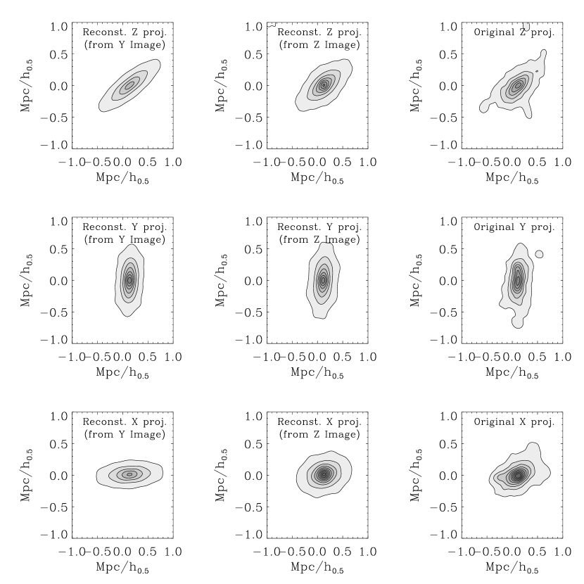
Figure 7: We determine the inclination angle by requiring consistency in the deprojection of the y-projection of the X-ray and SZ images. Using this, we predict the orthogonal projections of the surface density maps and compare with the true distributions. The left panels display the predicted x- y- and z- projections where the input image was taken to be the ‘observed’ y-projection SZ and X-ray images (and $\theta_{i}=32.^{\circ}$). The middle panel shows the result where the input image was taken to be the ‘observed’ z-projection SZ and X-ray images (and $\theta_{i}=84.^{\circ}$). The right panel shows the true underlying total mass distribution.

For an inclination angle of $32^{\circ}$ the COI covers most of k-space and one is forced to heavily rely on the assumed model to compensate for the lost information. As another example we deproject the z-projection image which has, for a prolate cluster, a rather large inclination angle, $\theta_{i}\approx 84^{\circ}$, and therefore has a negligible COI. The reconstructions from the z-projection maps are shown in the left panels of Figures 7, 8 and 9. Due to the minor COI extrapolation in this case the cluster center and geometry are better recovered and the other two projections are well predicted, even in the innermost region of the cluster.

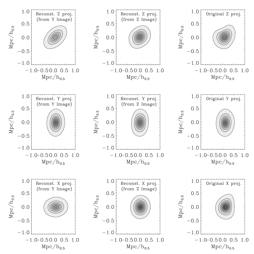
Figure 8: The same as in Fig. 7 but for the SZ maps

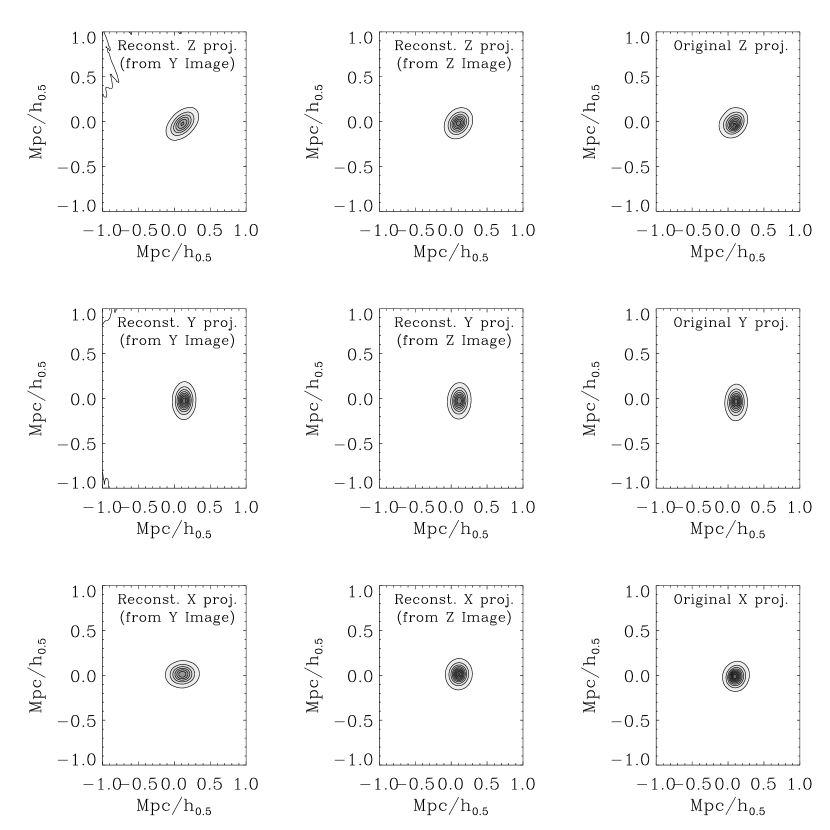
Figure 9: The same as in Fig. 7 but for the X-ray maps

Figure 10 shows the same comparison shown in the left panels of Figure 7 but for an oblate cluster. In this case the reconstructed x-projection is rather poorly predicted, supporting our contention regarding the cluster prolateness.

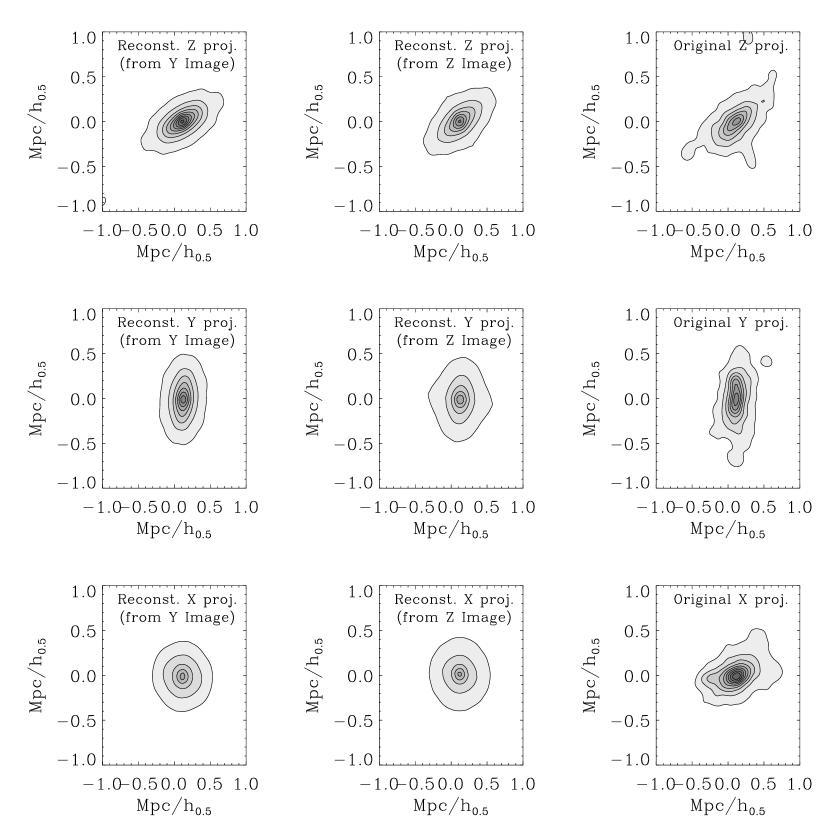
Figure 10: The same as Fig. 7; but assuming an oblate cluster

4.2.4 Comparison with the True 3D Distributions

Since we have the full 3D information from the simulations, we can robustly test the accuracy of the deprojection by comparing the deprojection with the true 3D gas or total mass distributions. In Figure 11, we deproject the X-ray and SZ images as a function of inclination angle. We transform the deprojected X-ray image to calculate the gas density from the deprojection, and compare with the true gas density by forming the normalized absolute difference:

$$\Delta(\theta_{i})=\sum\frac{|\rho^{\rm X-ray}_{\rm gas}(r,z)-\rho^{\rm true}_{\rm gas}(r,z)|}{|\rho^{\rm X-ray}_{\rm gas}(r,z)+\rho^{\rm true}_{\rm gas}(r,z)|},$$ (10)

where the $\rho^{\rm true}_{\rm gas}(r,z)$ is the true (axi-symmetrized) density field in the simulation.

In the left and middle panels of Figure 11, the dashed line displays the normalized absolute difference between the inferred and true gas densities as a function of inclination angle. For comparison, we also display (solid line) the difference between the gas density inferred from the X-ray deprojection versus that from the SZ – this mimics the procedure one would do in practice with real data, as discussed in §4.2.3. For this cluster, the agreement between the two is superb, especially under the assumption of a prolate cluster, demonstrating the reliability of the inclination angle determination (within $\lower 2.15277pt\hbox{$\;\buildrel<\over{\sim}\;$}\pm 5^{\circ}$) even in the case of a very wide COI.

Figure 11: The accuracy of the method: The dashed line displays the cumulated, normalized absolute difference between the inferred and true gas densities (where ‘true’ is the gas density obtained directly from our knowledge of the 3D distribution in the simulation data) as a function of inclination angle. For comparison, we also display (solid line) the difference between the gas density inferred from the X-ray deprojection versus that from the SZ – this mimics the procedure one would do in practice with real data. Left and middle panels show the result for prolate and oblate cluster assumption, respectively. Right panel: The same as before but with the comparison carried out with X-ray and SZ images that have realistic noise and resolution levels (§4.2.6).

A useful way to quantify the quality of the deprojection is to is see how well the radial profiles as calculated from the full and deprojected 3D distributions compare. In Figure 12 we calculate the radial profiles of the gas distribution and dark matter distribution. In both cases the reconstruction underestimated the density at the inner most center of the cluster but it yields a very accurate profile at radii $\gtrsim 0.3\;h_{0.5}^{-1}{\rm Mpc}$ for the gas density profile and $\gtrsim 0.5\,h_{0.5}^{-1}{\rm Mpc}$ for the dark matter density profile. The discrepancy between the real and reconstruction radial profiles in the innermost region, especially in the dark matter radial profile, is primarily due to the loss of the high frequency information in the COI, coupled with the finite resolution of the ‘observed’ maps. However, the total gas and mass differences are only of the order of few percent.

Figure 12: Left panel: The spherically averaged gas-density as a function of radius as calculated from the 3D deprojected gas distribution (solid line) and from the real (N-body) 3D distribution (diamonds). Right panel: The same as in the left panel but for the dark matter radial profile.

4.2.5 The Effect of Filling the COI on the Deprojection

In the full deprojection results shown until now, we have filled the COI by extrapolating an isothermal ellipsoidal profile that best fits the data outside the COI to within the COI. Here, we explore the effect of two different schemes for filling the COI. In the first scheme we simply let the values within the COI to smoothly (i.e., exponentially) drop to zero. The second scheme is to simply perform a linear extrapolation into the COI with the amplitude fixed by the value at the cone boundary (see Figure 4).

The general effect of first scheme is twofold. First, it results in a decrease in the amplitude of reconstructed source function, with the magnitude of the drop depending on the size of the COI. Second, it produces a double lobed shape distribution. As well, the second scheme results in a decrease in the amplitude of the reconstructed source function, and in more boxy shaped structures.

Figure 13 shows the predicted images obtained by projecting the 3D reconstructed SZ source function into x-, y-, and z-directions. Here we use the y-projected SZ as the input image for the algorithm. The inclination angle here is $32^{\circ}$ which means that the COI is quite wide. As expected, the re-projected y-image has the same quality as the comparable image (first column and second row) in Figure 8. The other two re-projected images show in both cases a drop in the amplitude and in the case of “constant filling” the reconstruction has a more boxy features while the “zero filling” results in a double lobed reconstruction.

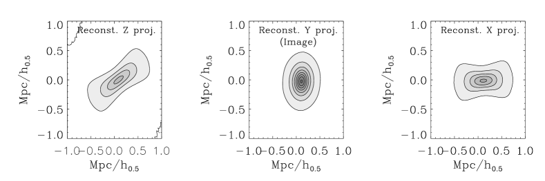
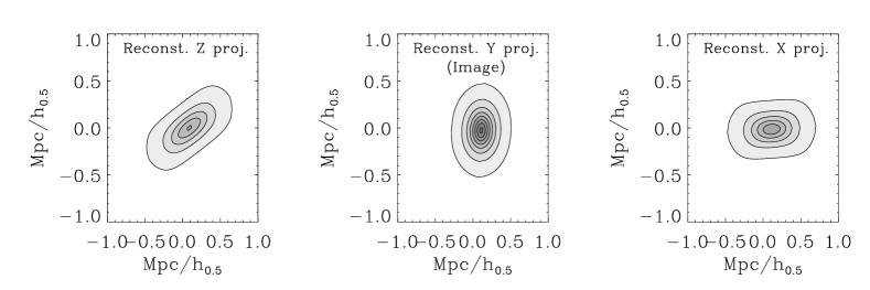
Figure 13: Upper row: Similar to the first column in Figure 8 but with the COI filled with values fixed to its boundary. Lower row: The same as the upper panels but with the COI filled with values that smoothly drop to zero.

4.2.6 Addition of Realistic Noise and Spatial Resolution

We have demonstrated thus far that our procedure for filling the COI and comparing the X-ray and SZ maps is sufficient to uniquely determine the inclination angle and hence determine the underlying 3D density structure. However, our calculations thus far have employed essentially infinite spatial resolution, and have been noise-free. In order to test if the method will be viable with realistic noise and instrumental response, we performed the following simple simulation: The SZ maps have been degraded to obtain $50^{\prime\prime}$ spatial resolution and peak $S/N\simeq 20$ similar to the resolution and sensitivity of the SZ observation attained at the OVRO and BIMA arrays (Carlstrom et al. (1995)). Similarly, the X-ray images have been degraded to spatial resolution of $10^{\prime\prime}$, and peak $S/N\simeq 10$, mimicking the resolution and sensitivity of CHANDRA for a rich cluster of galaxies.

The right panel of Figure 11 shows the angle determined from the X-ray vs. SZ maps comparison. The maps are initially denoised with a wavelet denoising algorithm (see Paper I; Brosch & Hoffman 1999; Hoffman 2000) and then the deprojected X-ray and SZ images are compared as a function of inclination angle. The best fit inclination angle in this case is $26^{\circ}$ which is within $6^{\circ}$ from the angle obtained from noiseless images; this is an excellent agreement that shows the potential of this method when applied to real data.

5 Testing the Method with the Full Simulated Cluster Sample

In Figure 14 we display the logarithmically scaled mass surface density, X-ray surface brightness, SZ decrement and emission weighted temperature distributions for the three orthogonal projections of the cluster at $z=0.3$. As before, the dimensions for the surface density, temperature and SZ decrement are physical ($M_{\odot}/{\rm Mpc}^{2}$ and $K$ for the first two, while the SZ decrement is dimensionless), while we recall that the X-ray surface brightness was calculated as the line of sight integral $\int\rho_{\rm gas}^{2}T^{1/2}dl$ and has dimensions $M_{\odot}^{2}K^{1/2}/{\rm Mpc}^{5}$. Figures 15 and 16 show the same plots for the cluster at $z=0.6$ and $z=0.9$ respectively.

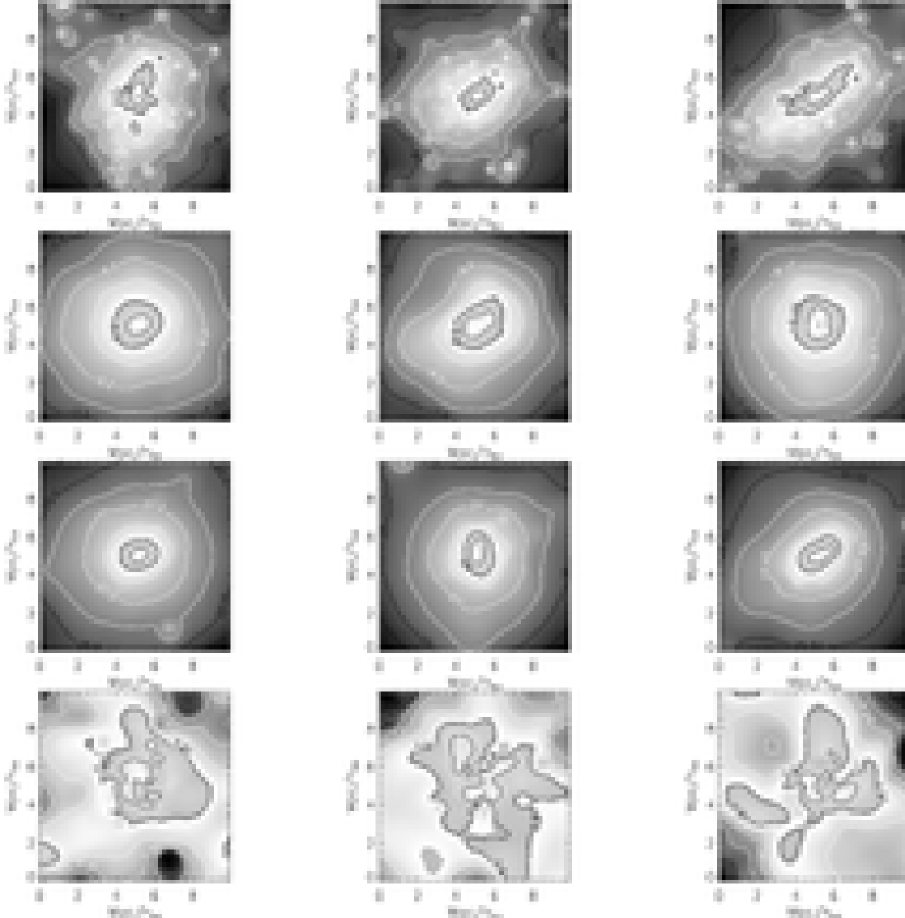
Figure 14: Left column: The x-projection for the prototype cluster at $z=0.3$. The grey scale and contours show the logarithmic intensity. Surface density (first panel; $M_{\odot}/{\rm Mpc}^{2}$), and Sunyaev-Zel’dovich decrement (second panel). X-ray surface brightness (third panel; $M_{\odot}^{2}K^{1/2}/{\rm Mpc}^{5}$), and emission weighted temperature (fourth panel; $K$). The middle and right columns display the same plots, but for the y- and z-projection maps respectively.

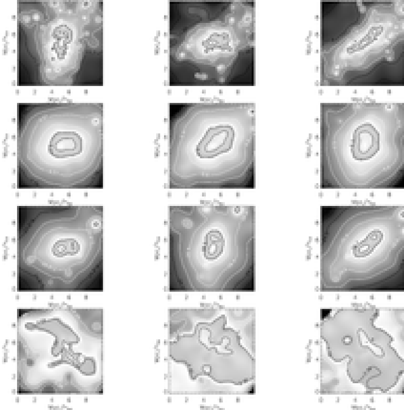
Figure 15: Left column: The x-projection for the prototype cluster at $z=0.6$. The grey scale and contours show the logarithmic intensity. Surface density (first panel; $M_{\odot}/{\rm Mpc}^{2}$), and Sunyaev-Zel’dovich decrement (second panel). X-ray surface brightness (third panel; $M_{\odot}^{2}K^{1/2}/{\rm Mpc}^{5}$), and emission weighted temperature (fourth panel; $K$). The middle and right columns display the same plots, but for the y- and z-projection maps respectively.

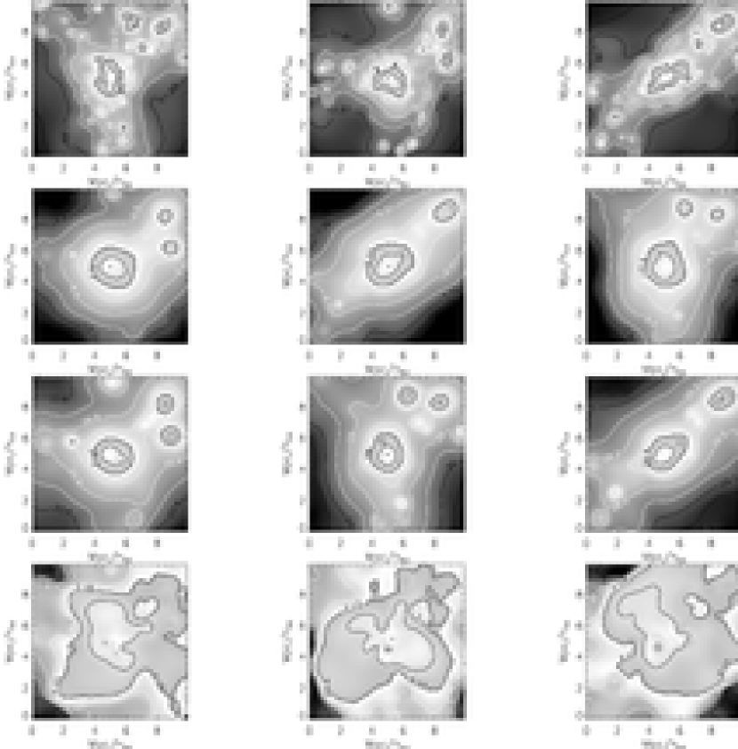
Figure 16: Left column: The x-projection for the prototype cluster at $z=0.9$. The grey scale and contours show the logarithmic intensity. Surface density (first panel; $M_{\odot}/{\rm Mpc}^{2}$), and Sunyaev-Zel’dovich decrement (second panel). X-ray surface brightness (third panel; $M_{\odot}^{2}K^{1/2}/{\rm Mpc}^{5}$), and emission weighted temperature (fourth panel; $K$). The middle and right columns display the same plots, but for the y- and z-projection maps respectively.

The merger history of the cluster can be traced through this series of simulation outputs. At $z=0.9$, the central mass concentration is in place, while two large sublumps are infalling at a projected co-moving distance of $\simeq 4\,h_{0.5}^{-1}{\rm Mpc}$ from the cluster center. At $z=0.6$, the entire system undergoes a major merger event. The three main mass concentrations are most clearly seen in the cores of the x- and y-projections (Figures 16 and 15), while the morphology of both the gas and dark matter in the z-projection becomes highly elliptical (Figure 14). This particular simulation output provides the most stringent test for the deprojection method: the system is clearly far away from dynamical equilibrium and certainly is very poorly described by a spherical model for the underlying gas and dark matter distributions. Nevertheless, as we shall demonstrate, the system is fairly well described as axially symmetric; the symmetry is qualitatively evident in the SZ and X-ray images, and, to a lesser extent, in the surface mass distributions.

Figure 17: The ratio of the z-integrated gas density and dark matter density, $\rho^{z}_{gas}/\rho^{z}_{DM}$ (solid lines), and the corresponding gas to dark matter mass ratio (dashed line), as a function of r, calculated from the surface density and Sunyaev-Zel’dovich maps of the z = 0 output. The left and right panels are produced assuming a prolate and oblate cluster respectively.

Figure 18: As in Figure 17 but for the z = 0.3 output.

5.1 The Baryon Fraction for All Clusters

Using equation (2), we calculated the gas to total mass and density ratios for the full suite of cluster outputs. The results are shown in Figures 17, 18, 19, and 20 for the simulation outputs at $z=0.0,0.3,0.6,\;{\rm and}\;0.9$ respectively.

In all cases, the method recovers very well the simulation input baryon fraction. The radial dependence of the gas to total mass ratio is flatter under the assumption of prolateness in the underlying 3D structure. Therefore, one can possibly use the expected small variability in gas to mass ratio to determine whether the cluster is prolate or oblate. In all the cases we examined, the gas to mass ratio shows less variability when its shape is assumed to be prolate, which is in total agreement with the real distribution of the gas and mass in those clusters.

Figure 19: As in Figure 17 but for the z = 0.6 output.

Figure 20: As in Figure 17 but for the z = 0.9 output.

5.2 The Inclination Angle

The inclination angle determination from the cluster SZ vs. X-ray images at the high redshifts is somewhat more complicated. This complication stems from the fact that at higher redshifts the cluster is not very relaxed, especially at $z=0.6$ where the cluster undergoes a major merger, rendering the connection between the images and the temperature uncertain. Nevertheless, we have attempted to reconstruct assuming a constant cluster temperature, chosen to be the mean temperature in the region around the cluster center with ‘intensities’ larger the $30\%$ of the image maximum density. We note that the scatter around that mean temperature in the chosen region is about $15\%$ at worst. Figure 21 shows the inclination angle as determined from a comparison of the SZ and X-ray images as viewed from the x, y and z-projections and at four different redshifts vs. the inclination angle as determined from the actual 3D distribution. The agreement between the two is very good.

Figure 21: The inclination angle as determined from the SZ vs. X-ray for each of the x,y, and z-projection images at four redshifts (12 clusters) drawn against the inclination angle as determined from the full real 3D distribution. The cluster at each redshift is marked with different symbols.

Obviously, filling the COI with an elliptical isothermal density becomes unrealistic for the $z=0.6$ case, where a major merger is taking place. In principle, one can vary the density model adopted for filling the COI. Here we choose to stay with the isothermal model with the hope of obtaining a reasonable reconstruction the cluster central region. Figures 22, 23 and  24 shows how well the method performs in the various redshifts when the z-projection images are used for reconstruction. Note the reconstruction is reasonable in all cases with the exception of the $z=0.6$ case where the details are different.

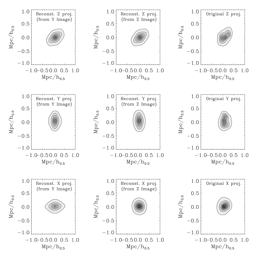
Figure 22: Similar to Fig. 8 (reconstruction from y & z-projection SZ maps); but with the cluster at redshift 0.3

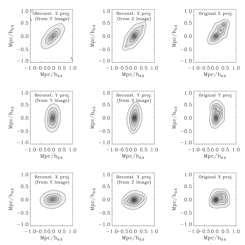
Figure 23: Similar to Fig. 8 (reconstruction from y & z-projection SZ maps); but with the cluster at redshift 0.6

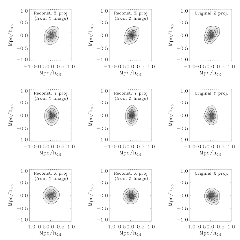
Figure 24: Similar to Fig. 8 (reconstruction from y & z-projection SZ maps); but with the cluster at redshift 0.9

6 Discussion

We have tested a method for deprojecting realistic galaxy cluster X-ray, SZ decrement and mass surface density maps, assuming only that the underlying gas/mass distributions are axially symmetric.

Conceptually, the deprojection procedure is straightforward: we first determine the image axis of symmetry, employing three different estimators accounting for the Poisson nature of the noise, and a technique giving increased weight to counts at large radii from the cluster center. Having a solution for the projected symmetry axis, we deproject the SZ, X-ray and surface mass distributions using equation (3), allowing for the possibility that the cluster is either oblate or prolate. As the inclination angle is the primary unknown, we deproject each image over a wide range of assumed inclination angles, searching for the angle that consistently yields the best reconstructed ratios between the Sunyaev-Zel’dovich, X-ray and the total mass deprojections.

At each inclination angle, we fill the information lost in the COI by either an elliptical isothermal model fitted to the data outside the COI, or a linear extrapolation into the COI with the amplitude fixed by the value at the cone boundary. The results are fairly insensitive to the precise algorithm applied to fill the COI, primarily because the information lost inside the COI is restricted to moderately high spatial frequencies.

For this study, we demonstrated this procedure in depth for a single, prototype cluster, and then applied the method to the entire sample. We demonstrated the goodness and robustness of the inclination angle determination in several ways: we compared the 3D gas density distribution as inferred from the SZ and X-ray deprojection, using the appropriate best fit angle for each case. The agreement between the two, in terms of both shape and amplitude, is very good (with a $5-10\%$ difference at the center).

We also determined the inclination angle by calculating the cumulated, normalized absolute difference between the inferred and true gas densities as a function of inclination angle (see Figure 11). The results agreed with our previous determinations to an accuracy of $\lower 2.15277pt\hbox{$\;\buildrel<\over{\sim}\;$}\pm 5^{\circ}$, demonstrating the reliability of the inclination angle determination even in the case of a very wide COI.

With the prototype cluster, we mimic observations of a rich galaxy cluster by CHANDRA (X-ray) and BIMA or OVRO (SZ) by degrading the resolution of the simulated data and adding noise. We again compared the deprojections of the two maps to determine the inclination angle and found $26^{\circ}$ (assuming a prolate cluster) which is within $6^{\circ}$ from the angle obtained from noiseless images; this is an excellent agreement that shows the potential of this method when applied to real data. We note here, that the purpose of this exercise is to show that the method has the potential of reproducing the 3D structure from the current data sets, this however does not mean that we have tested the application of the method to those data sets. The application of the method to each of those data sets and its unique specifications should be tested much more extensively, something we intend to carry out in a forthcoming study.

We also note, that since the current method is based on Fourier slice theorem it is well suited to analyze interferometric data, like the data obtained by the BIMA and OVRO experiments, where the raw data is given in the Fourier space U-V plane. For this kind of data one can for example, manipulate the X-ray or lensing data and transform them to the Fourier U-V plane and make the comparison with the SZ raw data at the wavenumbers covered in this plane which has the advantage of avoiding the U-V plane extrapolation needed in order to obtain a real space SZ image.

Finally, with the prototype cluster we tested the accuracy of the deprojection by comparing the true and inferred 3D radial profiles of the gas and total mass distributions (Figure 12). We found that the reconstruction underestimated the density at the innermost center of the cluster but it yields a very accurate profile at radii $\gtrsim 0.3\;h_{0.5}^{-1}{\rm Mpc}$ for the gas density profile and $\gtrsim 0.5\,h_{0.5}^{-1}{\rm Mpc}$ for the dark matter density profile. The discrepancy between the real and reconstruction radial profiles in the innermost region, especially in the dark matter radial profile, is primarily due to the loss of the high frequency information in the COI. However, the total, estimated over the whole the simulation volume, gas and mass differences are only of the order of few percent.

We also developed a feature of the method that provides a direct determination of the baryon fraction in clusters, independent of the cluster inclination angle. The only uncertainty comes from whether the underlying cluster gas density distribution is assumed to be prolate or oblate. For all of the clusters studied here, we note that the relative variations in the radial dependence for the baryon fraction for the prolate case are much smaller than if the cluster is oblate (see Figures 17, 18, 19, and 20). The shape of the baryon fraction radial profile provides an interesting possibility for discriminating between the prolate/oblate hypotheses: Due to the expected strong correlation between the gas and dark matter distributions, one expects their density and mass ratios to show relatively small variability as a function of radius from the cluster center. Indeed, for low- to intermediate redshift clusters $(z\lesssim 0.5)$, the baryon fraction has a relatively slight radial dependence $f_{b}(r)\propto r^{0.2}$ (Ettori & Fabian (1999)).

In conclusion, we have demonstrated that: 1) The fundamental assumption of axial-symmetry is a reasonable assumption when applied to a realistic subset of the general cluster population. 2) Under the assumption of axial symmetry, the method works very well for the purpose of recovering the 3D structure. 3) For a reasonable COI extrapolation scheme, the deprojection is robust, stable and unique even when most of k-space information has been lost in the projection. 4) The method is applicable for deprojecting cluster maps throughout the evolutionary history.

7 Appendix

The temperature decrement (the Sunyaev-Zel’dovich effect) the Rayleigh-Jeans regime due to upscattering of microwave background photons by the diffuse cluster electron gas in is given by

$$\frac{\delta T}{T}(x,y)=-2y=-2\frac{\sigma_{T}}{m_{e}c^{2}}\int n_{e}(\vec{r})\,k_{B}\,T_{x}(\vec{r})\,dl$$ (11)

where $\sigma_{T}$ is the Thompson cross section, $k_{B}$ the Boltzmann constant, $m_{e}$ is the electron mass, and $n_{e}(\vec{r})$ denotes the 3D electron gas distribution, with temperature $T_{x}(\vec{r})$.

The X-ray surface brightness in a given passband is given by

$$S_{X}(x,y)=\frac{1}{4\pi(1+z)^{3}}\int dl\,n_{e}^{2}(\vec{r})\Lambda(T_{x})$$ (12)

where the $\Lambda(T_{x})$ is the emissivity which is a function of the temperature and the energy passband at the cluster redshift.

These expressions can be rewritten in a general form, factoring out the normalization and 3D structural forms so that gas density an temperature are given by $n(x,y,z)=n_{0}f_{1}(\theta,\phi,\omega)$ and $T_{x}(\vec{r})=T_{x_{0}}f_{2}(\theta,\phi,\omega)$ where $D_{A}$ is the cluster angular diameter distance and $l=D_{A}\omega$. For galaxy clusters, the dominant emission mechanism is bremsstrählung in the limit of an optically thin plasma, so that $\Lambda\propto T_{x}^{1/2}$ and is a well-known function (Mewe et al. (1985); Mewe et al. (1986)). Thus we can write $\Lambda(T_{x})\simeq\Lambda_{0}(T_{x_{0}})\,f^{1/2}_{2}(\theta,\phi,\omega)$ and the SZ decrement can be written

$$\frac{\delta T}{T} = -2\,D_{A}\,\frac{k_{B}T_{X_{0}}}{m_{e}c^{2}}\sigma_{T}\,n_{0}\,\int f_{1}\,f_{2}\,d\omega$$ (13)

$$\equiv \Delta_{0}\;Q_{SZ}(f_{1},f_{2})$$

and

$$S_{X} = \frac{n_{0}^{2}\,\Lambda_{0}}{4\pi(1+z)^{3}}\;D_{A}\,\int f_{1}^{2}\,f_{2}^{1/2}\,d\omega$$

$$\equiv S_{X_{0}}\;Q_{X}(f_{1},f_{2}).$$

The combination of the SZ and X-ray observations affords the opportunity to determine the Hubble constant. The angular diameter distance to the cluster is given by

$$D_{A}=\frac{\Lambda_{0}}{16\pi(1+z)^{3}\sigma_{T}^{2}}\left(\frac{\Delta_{0}^{2}}{S_{X_{0}}}\right)\left(\frac{m_{c}c^{2}}{k_{B}T_{x_{0}}}\right)^{2}.$$ (15)

7.1 The isothermal $\beta$-model

Let us consider a concrete, analytical example. A convenient parameterization of the gas distribution is given by the standard $\beta$-model (e.g., Cavaliere & Fusco-Femaino (1976))

$$n_{e}(r)=n_{0}\left(1+\frac{r^{2}}{r^{2}_{c}}\right)^{-3\beta/2}.$$ (16)

Taking the further simplifying assumption of an isothermal gas, the form factors are given by

$$Q_{SZ} = \sqrt{\pi}\frac{\Gamma(3\beta/2-1/2)}{\Gamma(3\beta/2)}\theta_{c}\left(1+\frac{\theta^{2}}{\theta_{c}^{2}}\right)^{1/2-3\beta/2}.$$ (17)

and

$$Q_{X} = \sqrt{\pi}\frac{\Gamma(3\beta-1/2)}{\Gamma(3\beta)}\theta_{c}\left(1+\frac{\theta^{2}}{\theta_{c}^{2}}\right)^{1/2-3\beta}.$$ (18)

The required observations are the cluster redshift, a determination of the gas temperature, central density and a fit for $\beta$ and $\theta_{c}$.

We can slightly generalize the standard $\beta$-model, to allow for a more complicated 3D geometry. Consider as a toy-model a $\beta=2/3$, isothermal cluster with a gas density profile given by

$$\rho_{g}(x,y,z)=\frac{\rho_{g_{0}}\,r_{c}^{2}}{r_{c}^{2}+x^{2}/a^{2}+y^{2}/b^{2}+z^{2}/c^{2}}.$$ (19)

Without loss of generality, let us suppose the cluster z-axis forms an angle $\theta$ with respect to the line of sight. In this model, the Sunyaev-Zel’dovich decrement is given by

$$\frac{\delta T}{T} = -2\,\pi\,\frac{k_{B}T_{x}}{m_{e}c^{2}}\sigma_{T}\,n_{0}\,c^{\prime}\,r_{c}\,\biggl{[}1+\frac{x^{2}}{r_{c}^{2}a^{2}}+\frac{y^{2}}{r_{c}^{2}(c^{2}\sin^{2}\theta+b^{2}\cos^{2}\theta)}\biggr{]}^{-1/2}$$

$$= 2.5\times 10^{-4}\;c^{\prime}\;\biggl{(}\frac{r_{c}}{100\;{\rm kpc}}\biggr{)}\;\biggl{(}\frac{n_{0}}{0.01\;{\rm cm}^{-3}}\biggr{)}\;\biggl{(}\frac{T_{x}}{10\;{\rm keV}}\biggr{)}$$

$$\;\;\;\;\;\;\times\biggl{[}1+\frac{x^{2}}{r_{c}^{2}a^{2}}+\frac{y^{2}}{r_{c}^{2}(c^{2}\sin^{2}\theta+b^{2}\cos^{2}\theta)}\biggr{]}^{-1/2}$$

where

$$c^{\prime} = \biggl{(}\sin^{2}\theta/b^{2}+\cos^{2}\theta/c^{2}\biggr{)}^{-1/2}.$$ (20)

The observed surface brightness scales as

$$S_{X}(x,y) = \frac{n_{0}^{2}\,\Lambda_{0}}{4\pi(1+z)^{3}}r_{c}\;c^{\prime}\biggl{[}1+\frac{x^{2}}{r_{c}^{2}a^{2}}+\frac{y^{2}}{r_{c}^{2}(c^{2}\sin^{2}\theta+b^{2}\cos^{2}\theta)}\biggr{]}^{-3/2}\frac{{\rm\;erg}}{{\rm cm}^{2}{\rm s}}$$ (21)

It is immediately clear the error one makes when fitting a spherical isothermal $\beta$-model when the true underlying gas density follows this triaxial model. In the special case that $\theta=0^{\circ}$, then from equation (15), we find $\left(\frac{H}{H_{0}}\right)^{-1}=c$, where $H$ is the estimated value of the Hubble constant (see Figure 25).

We determine the error in the general case empirically. The value of $H_{0}$ extracted from SZ and X-ray observations assuming a spherical $\beta$ model will depend on the fitted values of the normalizations, $\beta$ and $r_{c}$.

Figure 25: The inferred value of the Hubble constant vs. the axis ratio, c, using the spherical $\beta$ model formalism, when the underlying surface density is triaxial. The model fit is done using $\chi 2$ minimization.

References

- Bardeen et al. (1986) Bardeen, J. M., Bond, J. R., Kaiser, N., & Szalay, A. S. 1986, ApJ, 304, 15
- Brosch & Hoffman (1999) Brosch, N., & Hoffman, Y. 1999, MNRAS, 305, 241
- Carlstrom et al. (1995) Carlstrom, J. E.; Joy, M.; Grego, L., 1995, ApJL, 456, L75.
- Cavaliere & Fusco-Femaino (1976) Cavaliere, A., & Fusco-Femaino, R. 1976, A&A, 49, 137
- Ettori & Fabian (1999) Ettori , S., & Fabian, A. C. 1999, MNRAS, 305, 834
- Evrard (1988) Evrard, A. E. 1988, MNRAS, 235, 911
- Fabian et al. (1981) Fabian, A. C., Hu, E. M., Cowie, L. L., & Grindlay, J. 1981, ApJ, 248, 47
- Fabricant et al. (1984) Fabricant, D., Rybicki, G., Gorenstein, P., 1984, ApJ, 286, 186
- Frenk et al. (1998) Frenk, C. S., White, S. D. M., Bode, P., Bond, J. R., Bryan, G. L., Cen, R., Couchman, H. M. P., Evrard, A. E., Gnedin, N., Jenkins, A., Khokhlov, A. M., Klypin, A., Navarro, J. F., Norman, M. L., Ostriker, J. P., Owen, J. M., Pearce, F. R., Pen, U.-L., Steinmetz, M., Thomas, P. A., Villumsen, J. V., Wadsley, J. W., Warren, M. S., Xu, G., & Yepes, G. 1999, ApJ, 525, 554
- Grego et al. (2000) Grego, L., Carlstrom, J. E., Joy, M. K., Reese, E. D., Holder, G. P., Patel, S., Cooray, A.R., & Holzapfel, W. L., 2000, ApJ, 539, 39
- Hoffman & Ribak (1991) Hoffman, Y., & Ribak, E. 1991, ApJ, 380, L5
- Mewe et al. (1985) Mewe, R., Gronenschild, E., & Oord, van den G. 1985, A&AS, 62, 197
- Mewe et al. (1986) Mewe, R., Lemen, J. R., & Oord, van den G. 1986, A&AS, 65, 511
- Nelder & Mead (1965) Nelder, J. A., & Mead, R. 1965, Computer Journal, 7, 308
- Press et al. (1992) Press, W. H., Teukolsky, S. A., Vetterling, W. T., & Flannery, B. P. 1992, in Numerical Recipes (Cambridge: Cambridge University Press), 694
- Yushikawa & Suto (1999) Yoshikawa, K., & Suto, Y. 1999, ApJ, 513, 549.
- Reblinsky & Bartelmann (1999) Reblinsky, K., & Bartelmann, M. 1999, in the proceedings of “Gravitational Lensing: Recent Progress and Future Goals”, Boston University, editors T.G. Brainerd and C.S. Kochanek.
- Zaroubi et al. (1998) Zaroubi, S., Squires, G., Hoffman, Y., & Silk, J. 1998, ApJ, 500, 87L