A Survey of FUSE and HST Sightlines through High-Velocity Cloud Complex C

Abstract

Using archival Far Ultraviolet Spectroscopic Explorer (FUSE) and Hubble Space Telescope (HST) data, we have assembled a survey of eight sightlines through high-velocity cloud Complex C. Abundances of the observed ion species vary significantly for these sightlines, indicating that Complex C is not well characterized by a single metallicity. Reliable metallicities based on [O I/H I] range from 0.1-0.25 solar. Metallicities based on [S II/H I] range from 0.1-0.6 solar, but the trend of decreasing abundance with H I column density indicates that photoionization corrections may affect the conversion to [S/H]. We present models of the dependence of the ionization correction on H I column density; these ionization corrections are significant when converting ion abundances to elemental abundances for S, Si, and Fe. The measured abundances in this survey indicate that parts of the cloud have a higher metallicity than previously thought and that Complex C may represent a mixture of “Galactic fountain” gas with infalling low-metallicity gas. We find that [S/O] and [Si/O] have a solar ratio, suggesting little dust depletion. Further, the measured abundances suggest an over-abundance of O, S, and Si relative to N and Fe. The enhancement of these $\alpha$-elements suggests that the bulk of the metals in Complex C were produced by Type II supernovae and then removed from the star-forming region, possibly via supernovae-driven winds or tidal stripping, before the ISM could be enriched by N and Fe.

1 Introduction

Almost four decades after their discovery (Muller, Oort, & Raimond 1963), the origin of high-velocity clouds (HVCs; Wakker & van Woerden 1997) remains a mystery. Defined by their incompatibility with a simple model of differential Galactic rotation, HVCs exhibit sub-solar metallicities and are currently favored to reside in the Galactic halo. Within this picture, it is not clear whether the source of HVCs is predominantly the accretion of low-metallicity gas onto the Galaxy (Wakker et al. 1999) or whether the material traces condensed outflows of hot enriched gas in a “Galactic fountain” (Shapiro & Field 1976; Bregman 1980). Intermediate-velocity clouds (IVCs), in contrast, exhibit solar metallicities and are thought to be of Galactic origin (Richter et al. 2001). Alternative hypotheses for the HVCs identify the majority of them as extragalactic objects within the Local Group at Galactocentric distances up to 500 kpc (Blitz et al. 1999), or posit that at least the subset known as Compact High Velocity Clouds (CHVCs) are extragalactic (Braun & Burton 1999). These objects would then be remnants of the formation of the Local Group. The statistics of moderate-redshift Mg II and Lyman limit absorbers (Charlton, Churchill, & Rigby 2000), would seem to rule out this hypothesis as a general scenario for group formation. In any event, the simulations which underpin the arguments for an extragalactic origin for the HVCs generally do not require such an identification for the very large complexes of HVCs, such as Complex C. However, within their model it is possible that Complex C might represent one of these building blocks viewed at a very close distance.

Complex C occupies nearly the same angular extent ($\sim 2000$ deg²) as the Magellanic Stream and consists of a number of separate HVC cores in the northern Galactic hemisphere. The Magellanic Stream has been linked to the Small Magellanic Cloud (SMC) through modeling of a tidal interaction with the Milky Way (Gardiner & Noguchi 1996) and through the similarity in metallicity of the Stream (0.2-0.3 solar; Lu et al. 1998; Gibson et al. 2000; Sembach et al. 2001) and SMC. In contrast, Complex C shows no obvious connection to the Galaxy. The distance to Complex C is at least 1.5 kpc (de Boer et al. 1994) from the non-detection of absorption lines toward high-latitude stars, although Wakker (2001) has recently put a new, albeit weak, lower limit at 6 kpc.

The lack of a strong distance constraint or evidence for interaction with the Galaxy make absorption-line studies of abundances in quasar sightlines the best option for gaining insight into the origin of Complex C. The first such study for Complex C, from HST Goddard High Resolution Spectrograph (GHRS) data along the Markarian 290 sightline by Wakker et al. (1999), inferred a metallicity of 0.1 solar based on the H$\alpha$-corrected [S II/H I] abundance. Those authors interpreted this abundance as evidence for infalling low-metallicity gas from the intergalactic medium (IGM) posited to explain the “G-dwarf problem.” Recently, however, other studies have demonstrated that the metallicity of Complex C varies from sightline to sightline. Gibson et al. (2001; hereafter G01) looked at all available archival GHRS and Space Telescope Imaging Spectrograph (STIS) data for five Complex C sightlines (including Mrk 290) and found that the metallicity inferred from the S II abundance varies between 0.1-0.4 solar, implying that Complex C may be contaminated by enriched gas from the Galactic disk. Other recent studies complicate the picture and further illustrate the point that Complex C may not be well described by a single metallicity. Richter et al. (2001a) combine FUSE and STIS data for the PG 1259+593 sightline and find an O I abundance of 0.1 solar, while Murphy et al. (2000) find an abundance of Fe II near 0.5 solar from FUSE observations of the Mrk 876 sightline.

The increasing availability of high-quality, far-ultraviolet FUSE and HST/STIS spectra has allowed the study of multiple transitions of the dominant ionization stages of N, O, Si, Fe, Ar, P, and S. In addition to estimates of the absolute abundances of these elements, the relative abundances of these elements can be inferred, sometimes more precisely than their absolute abundances. This allows a preliminary study of the depletion of refractory elements onto dust grains and the nucleosynthetic history of the gas.

Using HST-GHRS spectra, Savage & Sembach (1996) find that gas-phase abundances of refractory elements in the Galactic halo can be significantly depleted. For five halo sightlines, those authors find that the mean depletion from solar abundance is $\sim$ 0.3 dex for Si and $\sim$ 0.6 dex for Fe, while the S abundance is essentially solar. However, it is difficult to completely separate the effects of depletion from ionization effects. Although each element has a dominant ionization stage, no element is completely in one stage, and the fraction remaining in other stages varies with the element. As we show below, with enough measurements of different elements, it is possible to separate these two effects and assess the degree of depletion along sightlines toward Complex C.

Recent reviews have discussed the long history of exploiting relative abundances to reveal information about the chemical evolution of the gas (e.g., Pettini 2002; Matteucci 2002). Alpha-process elements (such as O, Ne, Si, and S) are produced predominantly by Type II supernovae (SNe), while Fe is produced primarily by Type Ia SNe. Nitrogen, however, is primarily produced by lower mass stars in the asymptotic giant branch (AGB) stage. With the bulk of $\alpha$-element production occurring relatively soon after star-formation is initiated, the release of N and Fe into the ISM can thus lag S or O enrichment by $\sim 250$ Myr (Henry et al. 2000). If the gas is somehow stripped from star-forming regions, either by a tidal interaction or in an outflow induced by combined SN-activity, then the resulting metal-content will be significantly N-poor. G01 and Wakker (2001) each interpret the low relative abundance of N in Complex C as evidence for primary enrichment by Type II SNe.

The cited Complex C abundance studies have all used different methods to infer metallicities of Complex C. Some studies fit the Complex C metal-line profiles with a Gaussian to determine the equivalent width, $W_{\lambda}$, while others simply integrate the profile over the Complex C velocity range established by the H I profile. These studies have also used different methods to determine species’ column densities, such as curve-of-growth (CoG) fitting, an apparent optical depth (AOD) calculation (Savage & Sembach 1991), or an assumption that these profiles are optically thin. In addition, except for the Richter et al. (2001a) work, these studies have typically concentrated on either FUSE or HST data alone. The FUSE data have the advantage that the covered spectral range includes numerous lines of O I, whose abundance is not as strongly influenced as S II by ionization effects (charge exchange keeps O I closely coupled to H I).

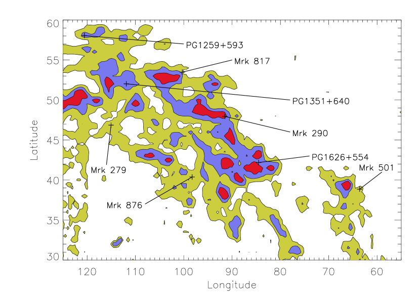
Figure 1: Contours of H I column density from the Leiden-Dwingeloo Survey (Hartmann & Burton 1997) for the high-velocity gas of Complex C ($-210\leq V_{LSR}\leq-95$ km s^-1). Contour levels are $N$(H I)$=1,3$, and $6\times 10^{19}$ cm^-2. The locations of the eight sightlines for this survey are labeled.

The goal of this work is to study all archival FUSE and HST data for sightlines through Complex C. Using a consistent method of analysis, we then determine abundances for the various metal species to infer information regarding the origin of HVC Complex C. The positions of the eight sightlines are shown in Figure 1, overlayed on H I emission data for Complex C from the Leiden-Dwingeloo Survey (LDS; Hartmann & Burton 1997). The FUSE and HST observations are discussed in § 2. Results for the analysis for the eight sightlines are presented in § 3. The results are discussed in § 4.

2 Observations

2.1 The FUSE data

The FUSE observations for these eight sightlines were obtained from the publicly available Multimission Archive (MAST) at the Space Telescope Science Institute. The total exposure times for FUSE observations towards the sightlines range from 8.3 ks for PG 1626+554 to 610.6 ks for PG 1259+593 and, as a result, data quality within the sample varies significantly. All sightlines were observed through the $30\arcsec\times 30\arcsec$ LWRS aperture in time-tag mode. A summary of the FUSE observations is shown in Table 1. For a complete description of the FUSE instrument and its operation see Moos et al. (2000) and Sahnow et al. (2000).

The raw data were obtained from the archive and calibrated spectra were extracted using a pass through the CALFUSE (v. 2.0.5) reduction pipeline. This version of the pipeline makes the correct transformation to a heliocentric wavelength scale. In versions earlier than 2.0, a sign error in file-header keywords resulted in the wrong heliocentric wavelength correction. In order to improve signal-to-noise for these data we include both “day” and “night” photons in the final calibrated spectra. The inclusion of “day” photons leads to strong airglow contamination of interstellar O I and N I absorption lines. However, the contamination is generally centered at $V_{LSR}=0$ km s^-1 and does not affect the higher-velocity Complex C absorption as confirmed by comparisons of unscreened spectra to spectra where “day” photons were screened by CALFUSE. Individual exposures were then coadded, weighted by their exposure times, to yield a final spectrum.

A single resolution element of the FUSE spectrum is about 20 km s^-1 ($\sim 10$ pixels) and, as a result data are oversampled at that resolution. Thus, to further improve signal-to-noise, data were rebinned over 3, 5, or 7 pixels depending on the initial data quality. A common problem with analysis of FUSE spectra is the setting of an absolute wavelength scale. The most common technique is to shift the wavelength scale by determining the velocity offset of line centroids from known absorption features. This was carried out by comparing the centroid of Galactic H I emission to various Galactic absorption features such as those of Ar I ($\lambda$1048.22, 1066.66), Fe II ($\lambda$1125.45, 1144.94), and H₂. We estimate the absolute wavelength scale to be accurate to within $\sim 10$ km s^-1.

2.2 The HST data

All available calibrated HST data for these sightlines were also obtained from MAST. The data consist of STIS and GHRS observations for seven of the sightlines. No HST spectroscopic data exist for PG 1626+554. See Table 2 for a summary of the HST observations. Final spectra were obtained by coadding individual exposures, weighted by their exposure times.

In order to both improve signal-to-noise and to match pixel size in velocity to that of the rebinned FUSE data, the HST data were rebinned to 3 or 5 pixels. In a few cases, data were not rebinned as the pixel sizes were already comparable to the rebinned FUSE data. Finally, the absolute wavelength scale was set as for the FUSE data, comparing the N I ($\lambda$1199.550) and S II ($\lambda$1250.584, 1253.811, 1259.519) lines to the centroid of Galactic H I emission.

3 Results

We detect metal-line absorption associated with Complex C in each of these sightlines. Individual line profiles were normalized by fitting low-order polynomials to the continuum in the region immediately surrounding the line in question. Regions within $\pm 3$ Å about the Galactic line-centroid were used for the continuum normalization, although in a number of cases spurious absorption near the line required the use of a much larger region for continuum measurement. For each sightline, the velocity range of Complex C is determined from the H I profile from the LDS data. The equivalent width, $W_{\lambda}$, of an absorption feature could then be measured by integrating the line over the velocity range occupied by Complex C. In the cases of Fe III $\lambda$1122.524 and N I $\lambda$1134.165, the complex C components are contaminated by the Galactic components of the Fe II $\lambda$1121.975 and $\lambda$1133.665, respectively. The contributions of these Fe II lines to the absorption feature were determined from a CoG fit to other Fe II lines integrated over the same velocity range. Uncertainties determined for the equivalent widths include error contributions from both photon statistics and continuum placement. In some cases, photon counting errors were estimated empirically from the data. For FUSE data, where individual lines are often measured in two different channels, equivalent widths are calculated by averaging values measured from the individual channels, weighted by a factor determined by their relative errors. When lines can not be measured, we estimate 3$\sigma$ upper limits to the line equivalent width.

In order to measure column densities of the various metal species, we fitted a CoG to the data. This requires the measurement of at least two lines for one species in each sightline. We are able to empirically determine a best-fit CoG for five of the eight sightlines. The three sightlines for which a CoG could not be fitted to the data have the lowest signal-to-noise, and the lines for which $W_{\lambda}$ can be measured are highly uncertain. Thus, to estimate column densities, and more often than not their upper limits, we adopt a CoG with doppler parameter $b=10$ km s^-1 for the lower quality data. This $b$-value is generally consistent with those obtained from the sightlines with the highest quality data. The doubly-ionized species of S and Fe typically reside in a different phase of the ISM than neutral and singly-ionized species and are thus not well described by a $b$-value determined from species of a lower degree of ionization. S III and Fe III in these sightlines have low measured values of $W_{\lambda}$, and their column densities are measured in the optically thin case (Spitzer 1978) by,

$$N(\mbox{cm}^{-2})=1.13\times 10^{17}\frac{W_{\lambda}(\mbox{m\AA})}{f\lambda_{0}^{2}(\mbox{\AA})}.$$ (1)

We adopt rest wavelengths and oscillator strengths from Morton (2002) except for several of the Fe II lines, where the oscillator strengths are from Howk et al. (2000).

A significant problem in determining the abundances of these various ions is in obtaining the H I column density of Complex C along these sightlines. H I columns cannot be determined from HST or FUSE data, as neutral hydrogen absorption in the Lyman series from Complex C is saturated and blended with saturated absorption from the Galaxy. A common approach in abundance studies is to adopt H I columns from 21-cm emission. However, beam sizes in the single-dish data are, at the smallest, of order a few arc-minutes compared to the subarc-second effective beams in HST and FUSE quasar absorption-line studies. Even over arc-minute scales, variations in H I columns can be significant (Wakker & Schwarz 1991) and if H I is clumped on scales of arc-seconds, then single-dish data will poorly reflect columns along quasar sightlines. Our approach then, is to adopt H I columns from the data of Wakker et al. (2001) taken at the Effelsberg 100-m telescope which, with a $9\arcmin.1$ beam, samples H I columns on a far smaller scale than the LDS 36$\arcmin$ beam. That survey includes H I profiles for all of our Complex C sightlines except PG 1626+554, where we measure the H I column from the LDS data. For these sightlines, the H I columns from the $9\arcmin.1$ beam range from 0.19 dex below to 0.28 dex above those of the 36$\arcmin$ beam. We adopt this range as the systematic error associated with the beam-size mismatch, although it should be stressed that the difference could be even greater when extrapolating to smaller scales. Future H I observations of Complex C at high spatial-resolution would be extremely useful to resolve this issue.

Metallicities are measured with respect to the solar (meteoritic) abundances of Grevesse & Sauval (1998; hereafter GS98). In addition, measured abundances from previous metallicity studies of Complex C are revised using the GS98 abundances so as to make reliable comparisons to our results. Holweger (2001) has recently presented new solar photospheric abundances, the most notable of which is a low value of [O/H]${}_{\sun}=5.45\times 10^{-4}$. The use of this abundance would increase our measured values of [O I/H I]_C by 0.094 dex. We use O I as a probe of cloud metallicity because the ionization state of oxygen is coupled to hydrogen through a resonant charge exchange reaction. Previous studies (Wakker et al. 1999; G01) have used [S II/H I]_C to probe metallicity, but have had to contend with ionization corrections, since, as we discuss in § 4.1, that quantity seems to depend on the photoionization correction as well as the actual sulfur metallicity.

In a number of cases we are unable to determine a metallicity based on [O I/H I]_C due to contamination of the O I $\lambda$1039.23 line by Galactic H₂ (5-0) R(2) Lyman absorption. In addition, the data quality for these particular sightlines precludes measurements of the weaker O I lines in the 920-950 Å range of the FUSE SiC channels. We can estimate the column density of O I along a given sightline at $N_{15}$(O I)$=(0.68)Z_{0.1}N_{19}$(H I), where $N_{n}$ is the column density in units of $10^{n}$ cm^-2 and $Z_{0.1}$ is the metallicity in units of 0.1 solar. Thus in cases where [O I/H I]_C could not be measured due to H₂ contamination, we estimate the expected equivalent width of the O I $\lambda$948.686 line based on the derived or assumed CoG for each sightline.

We have also made an attempt to measure molecular hydrogen in Complex C. Richter et al. (2001b, 2002) previously analyzed FUSE data for the PG 1259+593 and PG 1351+640 sightlines and were unable to detect high velocity H₂ associated with Complex C, whereas they find that molecular hydrogen is ubiquitous in IVCs where dust is more prevalent. In many cases we detect strong Galactic H₂ absorption, although H₂ associated with Complex C could not be measured within the sensitivity limits of the observations. FUSE is typically sensitive to H₂ column densities as low as $\sim 10^{14}$ cm^-2. In order to put upper limits on column densities of H₂, we measure 3$\sigma$ limits on $W_{\lambda}$ for the strong $J=0$ and $J=1$ Werner lines and assume that the lines are optically thin. Upper limits on molecular hydrogen column density as well as the molecular fraction, $f$(H₂)=2$N$(H₂)/[2$N$(H₂)+$N$(H I)], are shown in Table 3. Clearly there is very little molecular gas associated with Complex C.

Spectra for these eight sightlines, as well as line equivalent widths and the resulting column densities, abundances, and metallicities of the observed species are presented in §§ 3.1-3.8. Line profiles for O VI $\lambda$1031.93 are presented but not discussed. For a thorough discussion of high-velocity O VI from these and other sightlines see Sembach et al. (2002).

3.1 Mrk 279

Mrk 279 has good quality FUSE data with an average S/N of $\sim 9$ per pixel in the 1040-1050 Å range in the LiF1a channel. The GHRS data have been previously analyzed by G01, who determined a Complex C sulfur metallicity, revised assuming a GS98 solar abundance, of [S II/H I]${}_{\rm C}=-0.29\pm 0.18$ based on the measurement of S II $\lambda$1250 alone.

Profiles of some of the observed species are shown in Figure 2, along with the Effelsberg profile of H I emission. High-velocity H I emission is clearly present, though there appears to be significant blending with intermediate velocity components. Wakker et al. (2001) identify eight components to the full H I profile, two of which are at high velocity. We follow the approach of G01 and choose an integration range that spans these two components ($-180\leq V_{LSR}\leq-90$ km s^-1). Since there appears to be significant blending with an IVC, we directly integrate the Effelsberg H I profile to determine $N$(H I) over this range.

Equivalent widths for the Mrk 279 sightline are shown in Table 4. The S II $\lambda$1253 line could not be measured from the GHRS spectrum owing to contamination from a Ly$\alpha$ absorber intrinsic to Mrk 279. The S II $\lambda$1259 line is not included in the spectrum, and thus only S II $\lambda$1250 is reported. G01 raise the issue that an intrinsic Ly$\alpha$ absorber seen just redward of S II $\lambda$1250 may contaminate the line at higher negative velocities, although the equivalent width of the Complex C component and the implied S II metallicity are consistent with other sightlines in our survey.

We have measured the equivalent widths of five O I and four Fe II lines associated with Complex C. The data are best fitted by a CoG with doppler parameter $b=9.7^{+5.0}_{-2.8}$ km s^-1, as shown in Figure 3. Resulting column densities, abundances, and metallicities for the ion species are shown in Table 4. The implied metallicity for this sightline from the O I measurement is around $\sim 0.2$ solar, significantly lower than the $\sim 0.5$ solar measurement of G01 from S II data. We measure a S II metallicity closer to $\sim 0.6$ solar from the same data, and we suspect that ionization effects may play a role for that species (see § 4.1).

We note that the H I profile seems to indicate a significant blending of the lower-velocity Complex C component (centered at $V_{LSR}\sim-105$ km s^-1) with an IVC (centered at $V_{LSR}\sim-75$ km s^-1) known as IV9. IVCs typically have metallicities near solar, and our chosen integration range for Complex C may include absorption from IV9, thus biasing our measurements to higher metallicities. In order to test this, we have performed an abundance analysis of the higher-velocity Complex C component (centered at $V_{LSR}\sim-140$ km s^-1) using the integration range $-180\leq V_{LSR}\leq-120$ km s^-1. Results from this analysis are shown in Table 4, where values in parenthesis indicate measurements for the $-140$ km s^-1 component. The abundances of this component are similar to that of both components in the full integration range. The indicated metallicity based on O I is $\sim 15$% lower than in the case of the full integration range, indicating some contamination by IV9 in the range $-120\leq V_{LSR}\leq-90$ km s^-1. However, it should be noted that the O I abundance of this component indicates a metallicity of $\sim 0.17$ solar.

3.2 Mrk 290

The GHRS data for this sightline have been well studied by Wakker et al. (1999) and G01. Each group uses S II measurements to infer Complex C metallicities of about $\sim 0.1$ solar. The FUSE data are poor, consisting of only 13 ks of exposure time, and have an average S/N of only $\sim 1$ per unbinned pixel in the 1040-1050 Å range in the LiF1a channel.

Profiles of some of the observed species are shown in Figure 4, along with the LDS profile of H I emission. The LDS H I profile shows a clear demarkation between the Complex C and Galactic H I components. The integration range for equivalent width determinations is thus set by the extent of the Complex C component ($-165\leq V_{LSR}\leq-80$ km s^-1). The column density of H I along this sightline from the Effelsberg data is ($12.3\pm 0.6$)$\times$10¹⁹ cm^-2, the highest column sightline from this sample. Wakker et al. (1999) combined Effelsberg single-dish data with Westerbork Synthesis Radio Telescope (WSRT) interferometric data to measure $N$(H I)$=9.2\times 10^{19}$ cm^-2 at 1$\arcmin$ resolution. The high H I column, coupled with the poor quality of the currently available FUSE data, makes this sightline an obvious choice for further FUSE observations.

Given the data quality, we are only able to place upper limits on Complex C metallicities for species in the FUSE bandpass. In addition, strong Galactic H₂ (5-0) R(2) Lyman absorption blends with O I absorption from Complex C, limiting our measurement of that species to only an upper limit. Equivalent width measurements, column densities, abundances, and metallicities for the sightline are summarized in Table 5.

In order to measure column densities, we assume that the data can be fitted by a $b=10$ km s^-1 CoG, which adequately fits the S II GHRS measurements. Since the upper limits on the FUSE lines are quite high, located on the flat part of the CoG, we use equation 1 to calculate column densities from lines which are generally optically thin for the other sightlines, namely N I $\lambda$1134.17, Si II $\lambda$1020.70, and Ar I $\lambda$1048.22. The O I $\lambda$1039.23 and Fe II $\lambda$1144.94 lines do not satisfy the optically thin requirement for the other sightlines, and column densities from these lines are derived via the CoG method.

We obtain a similar S II metallicity as Wakker et al. (1999) and G01 for Complex C along this sightline, [S II/H I]${}_{\rm C}=$$-1.00^{+0.16}_{-0.15}$. Using the WSRT H I column would increase this value by 0.13 dex. Again, it is likely that the S II metallicity is not the ideal tracer of the true metallicity along this sightline. Measurements of the H₂/O I $\lambda$1039.23 blend place an unrestrictive upper limit to the metallicity along this sightline of $<0.6$ solar. It would be useful to study O I lines in the $920-950$ Å range to better constrain the metallicity. However, FUSE observations of this wavelength range require long exposures owing to the relatively low-sensitivity of the SiC1b and SiC2a channels. If the metallicity along this sightline lies in the range 0.1-0.25 solar, then the expected $W_{\lambda}$ of the O I $\lambda 948.69$ line, determined from the CoG, is within the range 100-115 mÅ.

3.3 Mrk 501

Existing FUSE data for this sightline are of generally poor quality with a S/N of $\sim 1.5$ per unbinned pixel in the $1040-1050$ Å range of the LiF1a channel. Due to the low signal-to-noise of the HST data, G01 were able to place only upper limits on S II metallicity.

Figure 5 shows some of the observed absorption profiles, along with the LDS profile of H I emission. The high-velocity component of the H I profile is not well-separated from Galactic and intermediate H I emission. The only sensible approach is to integrate over the two high-velocity H I components ($-135\leq V_{LSR}\leq-65$ km s^-1) identified by Wakker et al. (2001). The H I column density, ($1.6\pm 0.1$)$\times$10¹⁹ cm^-2, of Complex C along this sightline is the lowest among the sightlines in this sample.

Since Mrk 501 absorption features in both the FUSE and GHRS spectra cannot be measured above the noise, we place 3$\sigma$ upper limits on $W_{\lambda}$ for Complex C absorption features. Equivalent width, column density, abundance, and metallicity upper limits for the sightline are summarized in Table 6. The determination of column densities was carried out through a procedure analogous to that of the Mrk 290 data.

The upper limit of [O I/H I]${}_{\rm C}<$$-0.54$ places a useful limit on the metallicity at $<0.3$ solar. With slightly improved signal-to-noise through a longer FUSE exposure for this sightline, the O I metallicity could possibly be measured. Toward this end, we have planned a 55 ks exposure with FUSE during Cycle 3. The limit we place on the S II metallicity of [S II/H I]${}_{\rm C}<0.05$, near solar, is about 0.2 dex higher than the limit of G01.

3.4 Mrk 817

The FUSE data for Mrk 817 are of high quality, with a S/N of $\sim 11$ per unbinned pixel in the 1040-1050 Å range for the LiF1a channel. The GHRS data are also of good quality and were analyzed by G01, who measured a metallicity, revised assuming a GS98 solar abundance, of [S II/H I]${}_{\rm C}=$$-0.41\pm 0.07$ based on measurements of the S II $\lambda$1250 and $\lambda$1253 lines.

Figure 6 shows profiles of some of the observed species, as well as the LDS profile of H I emission. The Complex C component of the H I profile is clearly separated from the Galactic and intermediate-velocity components, and the range of integration is chosen to match the velocity range of the high-velocity component ($-140\leq V_{LSR}\leq-80$ km s^-1).

The measured values of $W_{\lambda}$ for the Mrk 817 sightline are shown in Table 7. The S II $\lambda$1250 and $\lambda$1253 lines are easily detected in the GHRS spectrum, although the stronger S II $\lambda$1259 line is just redward of the spectrum’s upper-wavelength cutoff. Determination of the local continuum associated with the S II $\lambda$1253 line is difficult owing to the superposition of the line with the Ly$\alpha$ emission line intrinsic to Mrk 817. The error associated with the uncertain continuum is not included in the value quoted for S II $\lambda$1253 in Table 7.

We fitted a CoG with doppler parameter $b=10.8^{+3.2}_{-2.2}$ km s^-1, shown in Figure 7, to equivalent width data for the five O I, six Fe II, and two S II lines. The resulting column densities, abundances, and metallicities for the ion species are shown in Table 7. The O I measurement implies a metallicity along this sightline of $\sim 0.25$ solar, nearly the same as that of the Mrk 279 sightline. Our measured value of [S II/H I]${}_{\rm C}=$$-0.34\pm 0.08$ implies a metallicity closer to $\sim 0.5$ solar, although as for Mrk 279 a photoionization correction may be necessary to obtain a true metallicity from S II measurements. It should be noted that, although the O I metallicity determined for the Mrk 817 sightline is consistent with the loose upper limit set for the Mrk 290 sightline, G01 argue that their disparate S II measurements cannot be reconciled by a single metallicity for Complex C.

3.5 Mrk 876

Archival FUSE data for Mrk 876 are of good quality, with a S/N of $\sim 6$ per unbinned pixel in the 1040-1050 Å range of the LiF1a channel. Unfortunately, this is not an optimal sightline for metallicity studies as it passes through a very large column of Galactic molecular hydrogen with N(H₂)=2.3$\times$10¹⁸ cm^-2 (Shull et al. 2000), strong absorption from which contaminates many of the most important Complex C absorption features. These data were originally presented by Murphy et al. (2000) who measured a metallicity, revised assuming a GS98 solar abundance, of [Fe II/H I]${}_{\rm C}=$$-0.31^{+0.15}_{-0.23}$. The STIS data for Mrk 876 include the N I $\lambda 1199.55$ line, although the S II lines are not covered by the spectral bandpass. G01 measured a surprisingly low N I metallicity for this sightline and argue for a differing nucleosynthetic history for the enrichment of sulfur and nitrogen.

Observed absorption line profiles are shown in Figure 8. The Effelsberg profile of H I emission, also shown in Figure 8, exhibits two high-velocity components in the velocity range $-210\leq V_{LSR}\leq-95$ km s^-1. This span is chosen as the integration range for the Complex C $W_{\lambda}$ measurements shown in Table 8. Owing to the strong Galactic H₂ absorption, we are unable to measure, or put meaningful upper limits on, the important O I $\lambda$1039.23 line. Other oxygen lines in the 920-950 Å range are difficult to measure within the sensitivity limits, partly due to the absence of data for the SiC2 channel.

From the available data, we are able to fit a CoG with $b=16.1^{+7.4}_{-3.9}$ km s^-1, shown in Figure 9, to the four observed Fe II lines. Resulting column densities, abundances, and metallicities for the ion species are listed in Table 8. We measure an Fe II metallicity of [Fe II/H I]${}_{\rm C}=$$-0.42^{+0.15}_{-0.12}$. Our N I measurement from $\lambda$1199.55 of [N I/H I]${}_{\rm C}=$$-1.09^{+0.16}_{-0.15}$ is greater than the G01 measurement of [N I/H I]${}_{\rm C}=$$-1.28\pm 0.09$ from the same data. The data quality in the SiC1b channel is insufficient to adequately measure O I absorption, though we are able to place a 3$\sigma$ upper limit on the metallicity based on [O I/H I]_C at $<0.5$ solar. However, we note that we are able to measure the O I $\lambda\lambda$929.52, 936.63 lines at the 2$\sigma$ level, indicating that the metallicity along this sightline may be relatively high. The absorption profile of the 929.52 Å line strongly hints at the two-component structure seen in H I. Higher quality FUSE data especially for the SiC channels, along with STIS observations over a larger bandpass for this target, would allow a far more complete investigation of metallicities along this sightline.

In an attempt to investigate the sub-component structure of Complex C absorption in this sightline, we have performed seperate abundance analyses of the components centered at $V_{LSR}\sim-175$ km s^-1 (integration range $-210\leq V_{LSR}\leq-150$ km s^-1) and $V_{LSR}\sim-130$ km s^-1 (integration range $-150\leq V_{LSR}\leq-95$ km s^-1). This is similar to the approach taken by Murphy et al. (2000) where these components were fitted separately. Results are presented in Table 8. Measurements of [Fe II/H I]_C for the $-175$ and $-130$ km s^-1 components are $-0.71^{+0.14}_{-0.15}$ and $-0.35^{+0.10}_{-0.09}$, respectively, suggesting that the lower velocity component may be of a significantly higher metallicity than the higher velocity component. If the lower velocity component is indeed at a smaller distance, then it is possible that it could have a higher degree of enrichment from the Galaxy. In addition, we are able to make tenuous measurements of the O I $\lambda\lambda$929.52, 936.63 lines in the lower-velocity component at $W_{\lambda}=$ 48$\pm$16 and 53$\pm$19, respectively, consistent with a metallicity near 0.3 solar. This value, however, is highly uncertain, and better quality data are necessary for confirmation.

3.6 PG 1259+593

Of these eight sightlines, the data for PG 1259+593 are of the highest quality. The FUSE data have an unbinned S/N of $\sim 8$ in the 1040-1050 Å range of the LiF1a channel, while the STIS spectrum covers useful absorption lines in the 1150-1700 Å range. The bulk of these data were recently analyzed by Richter et al. (2001a) who measured a metallicity from the O I lines of $\sim 0.1$ solar. The data presented here include an additional 400 ks of exposure time obtained with FUSE, which allowed us to refine these abundances and obtain a new measurement of Ar I.

Figure 10 shows some of the observed absorption profiles along with the LDS profile of H I emission. The H I profile shows a clear division between the Complex C high-velocity component, the intermediate-velocity component (the IV Arch), and the Galactic component. The integration range is thus set at $-155\leq V_{LSR}\leq-95$ km s^-1, with little chance that profiles are contaminated by intermediate-velocity gas. The metallicity of the IV Arch is considered by Richter et al. (2001a), who find solar abundances and conclude the cloud to be of Galactic origin. Measured values of $W_{\lambda}$ are shown in Table 9.

We have measured six O I, eight Fe II, four Si II, two S II, and two Si II lines to which we have fitted a CoG with $b=10.0^{+1.9}_{-1.5}$ km s^-1, shown in Figure 11. Richter et al. (2001a) empirically determined a similar value, $b=9.8^{+4.7}_{-1.2}$ km s^-1. Resulting column densities, abundances, and metallicities for the ion species are listed in Table 9. The Complex C abundances measured for this sightline are among the lowest of the sightlines in this sample. We confirm the result of Richter et al. (2001a) for O I  where we measure [O I/H I]${}_{\rm C}=$$-1.00^{+0.19}_{-0.25}$, implying a metallicity of $\sim 0.1$ solar. The S II abundance is also low, [S II/H I]${}_{\rm C}=$$-0.74^{+0.13}_{-0.13}$, with only the Mrk 290 sightline indicating a lower S II metallicity. The high quality of these new data allow a measurement of [Ar I/H I]${}_{\rm C}=$$-1.22^{+0.13}_{-0.16}$. This target is the only sightline for which a $>3\sigma$ detection can be made from Ar I $\lambda$1048.22.

3.7 PG 1351+640

Currently available FUSE data for this sightline are of fair quality, with an average S/N of $\sim 3$ in the 1040-1050 Å range for the LiF1a channel per unbinned pixel. However, the target was not observed by the SiC1 channels thus limiting our ability to detect absorption at $\lambda\lesssim 990$ Å. The STIS data are of good quality, although the spectral range of the observations (1195-1299 Å) is more limited than the STIS data for PG 1259+593.

The observed absorption profiles, along with the LDS profile of H I emission, are shown in Figure 12. The high-velocity H I component of the profile appears to be separated from the prominent intermediate-velocity feature, and we choose the integration range of Complex C to span the extent of the high-velocity emission ($-190\leq V_{LSR}\leq-95$ km s^-1). Measured values of $W_{\lambda}$ are shown in Table 10. The O I $\lambda$1039.230 Complex C feature is contaminated by Galactic H₂ (5-0) R(2) Lyman absorption, and thus only an upper limit to the Complex C contribution can be established. In addition, poor data quality in the SiC channels precludes any determination of O I abundance based on the 920-950 Å lines. Further FUSE observations would obviously be very helpful. In the STIS spectrum, strong absorption features of unknown origin coincide with the Complex C components of N I $\lambda$1199.55 and S II $\lambda$1259.52, although we are able to measure the S II $\lambda$1253.80 line.

We have used the two detected Fe II lines to determine a best-fit CoG with $b=13.7^{+3.3}_{-2.5}$ km s^-1. Resulting column densities, abundances, and metallicities for the ion species are listed in Table 10. We measure an abundance [Fe II/H I]${}_{\rm C}=$$-0.45^{+0.26}_{-0.17}$, which is among the highest of the sightlines in this sample. The upper limit placed on the metallicity based on the O I $\lambda$1039.23/H₂ blend is at $<0.5$ solar. Limits on N(O I) based on lines in the SiC channels do not improve on this value. We expect a value of $W_{\lambda}$ in the range 100-130 mÅ, corresponding to a metallicity range of 0.1-0.25 solar, for the O I $\lambda 948.69$ line. The upper limit [S II/H I]${}_{\rm C}<$$-0.49$ is consistent with the trend we observe in this sample for [S II/H I]_C versus $N$(H I).

3.8 PG 1626+554

The FUSE data for this final target in our sample are poor, with an average S/N of $\sim 1.2$ per unbinned pixel in the 1040-1050 Å range. The data consists of only 8.3 ks of exposure time, the shortest exposure in this sample. In addition, GHRS or STIS data for this target do not exist. Observed absorption profiles are shown in Figure 14 along with the LDS profile of H I emission. The H I profile shows a prominent high-velocity component, well-separated from lower-velocity emission, spanning the velocity range of $-155\leq V_{LSR}\leq-75$ km s^-1. This target is not included in the Wakker et al. (2001) Effelsberg survey, so we use the LDS data to measure a neutral hydrogen column of the high-velocity component, $N$(H I)$=(6.2\pm 0.4)\times 10^{19}$ cm^-2. We note that the systematic error associated with abundance measurements in this sightline are quite high due to the large beam size for the $N$(H I) measurement.

Owing to data quality, we are unable to make a 3$\sigma$ detection of any of the Complex C absorption features; the most significant detection is the Fe II $\lambda$1144.94 line at the 2$\sigma$ level. The O I $\lambda$1039.23 feature is prominent, but strong Galactic H₂ contamination is likely. Given the possible H₂ contamination, it would be useful to obtain high-quality SiC data to analyze O I lines in the 920-950 Å region. The O I $\lambda 948.686$ line is expected to have a $W_{\lambda}$ value in the range 80-100 mÅ, corresponding to a range in metallicity of 0.1-0.25 solar. Measurements of equivalent width, column density, abundance, and metallicity are summarized in Table 11. Column densities were determined as for Mrk 290.

The upper limit of [O I/H I]${}_{\rm C}<$$-0.79$ is quite low and, aside from the uncertain $N$(H I) from the LDS data, suggests that the metallicity may be close to that of the $\sim 0.1$ solar value along the PG 1259+593 sightline. The Fe II upper limit is also quite low, and the 2$\sigma$ measurement of the 1144.939 Å line at $W_{\lambda}$= 81$\pm$39 suggests an Fe II abundance below 0.1 solar. Clearly this is an interesting sightline for further FUSE and HST observations, along with higher-resolution H I data.

4 Discussion

4.1 Ionization Effects on Elemental Abundances

For the eight sightlines, we have calculated abundances of various ion species, O I, S II, Fe II, Si II, and N I, which are the dominant ionization states in warm neutral clouds. However, there are certain to be regions in these clouds with ionized hydrogen. As a result, the measured column of H I does not fully reflect the total column of H along the line of sight. This is not a problem for elements such as N or O, where the ionization state is coupled to that of H through charge-exchange interactions. Elements such as S and Si, however, are certain to be singly-ionized in both H I and H II regions. Therefore, in order to make definitive statements regarding elemental abundances, one must take into account possible photoionization corrections to ion abundances.

In Figure 15, we have plotted the runs of S II, Si II, Fe II, and O I abundance versus $N$(H I). The abundance [S II/H I], and to a lesser extent [Si II/H I], shows a trend of decreasing abundance with column density. If one assumes that the elemental abundance does not vary significantly as a function of column density, then such a trend can be explained by an ionization effect.

In order to model the effect of column density on ion abundances, we have generated a grid of photoionization models using the code CLOUDY (Ferland 1996). We make the simplified assumption that the absorbing gas can be treated as plane-parallel slabs illuminated by incident radiation dominated by OB associations. The models assume a $T=35,000$ K Kurucz model atmosphere and a cloud metallicity of $Z_{\sun}=0.1$. While the extent of the incident ionizing field on Complex C is not well known, H$\alpha$ emission measures of Complex C have been argued (Bland-Hawthorn & Putman 2001; Weiner et al. 2002) to be consistent with radiation from our Galaxy at the level of log $\phi\approx 5.5$ (photons cm^-2 s^-1), which we assume as the normally-incident ionizing flux in the models. For three assumed gas volume densities, $n_{\rm H}$, we calculate the logarithmic difference between [X^ion/H I] and [X^element/H] versus $N$(H I), shown in Figure 16 for S, Si, and Fe. We find that the ionization corrections necessary for O and N are negligible, and that [O I/H I]_C and [N I/H I]_C should reflect actual values of [O/H] and [N/H]. It would be useful to check this for N by measuring Complex C N II $\lambda 1084$. However, this absorption feature cannot be measured in these sightlines since it is saturated and blended with saturated Galactic absorption.

Given the simplified nature of these models and the uncertainty in the actual gas densities, these models are for illustrative purposes only and are designed mainly to explain the general trend observed in the ion abundances versus H I column. The models show that the spread in values of [S II/H I]_C observed in these sightlines is more a reflection of ionization conditions in the cloud than actual variations in [S/H]. A similar statement can be made for the [Si II] trend. For the intermediate density model ($n_{\rm H}=0.03$ cm^-3), the ionization correction to the [S II/H I]_C puts those values more in line with the [O I/H I]_C measurements. Fe is not subject to as large a photoionization correction, which may explain the lack of a strong trend in [Fe II/H I]_C versus $N$(H I).

4.2 The Origin of Complex C

In Table 12, we show the measured abundances, relative to solar, of O I, S II, Fe II, Si II, and N I. As demonstrated in § 4.1, many of these ion species’ abundances are subject to ionization corrections in order to convert to elemental abundances. Oxygen and nitrogen are particularly insensitive to such effects, and the values listed should accurately reflect the true values of [O/H]_C and [N/H]_C.

We find that the metallicity of Complex C ranges from 0.1-0.25 solar for the three sightlines in which O I could be measured. The upper limits on [O I/H I]_C established for the other sightlines are consistent with such a range. As stated by G01, the moderate abundances imply that Complex C is unlikely to be representative of purely infalling extragalactic gas. Further, we find that the metallicity varies from sightline to sightline; the [O I/H I]_C and ionization-corrected [S II/H I]_C, within their $1\sigma$ error bars, suggest variations by factors of 2-3. Although N is produced through different mechanisms than O, the two cases for which N I could be measured differ in abundance by 0.7 dex, further suggesting that Complex C cannot be characterized by a single metallicity. Metallicities in the range 0.1-0.3 solar are characteristic of tidally-disrupted dwarf-satellites (LMC and SMC) or gas in the outer disk ($>1.5R_{\sun}$) of the Galaxy (Gibson 2002). While the calculated metallicities are still somewhat low to assign a Galactic origin, it is tempting to assign a mixed origin to Complex C, with gas of Galactic (and/or satellite) origin blending with infalling low-metallicity clouds. If this is the case, one might expect, with better data, to see a trend of lower metallicity with higher $N$(H I), since the mixing of infalling gas with enriched Galactic disk gas may take considerable time. The interpretation of Complex C metallicity may therefore depend on the alignment of the background AGN with the cloud core or halo. We suggest that further FUSE and HST observations of many of these sightlines, together with higher-resolution 21-cm H I maps, will more completely address these issues.

In order to further explore issues concerning the origin of Complex C, we have calculated elemental abundances relative to O I. We consider data only from the three sightlines (Mrk 279, Mrk 817, and PG 1259+593) for which an O I column density could be measured. Figure 17 shows measured values of [S II/O I], [Si II/O I], [Fe II/O I], and [N I/O I], where we have plotted the column density weighted mean values for the three sightlines. The upper limit for [N I/O I] is taken as the least restrictive of the limits from the various sightlines.

Using the ionization corrections discussed in § 4.1 for the intermediate density model ($n_{\rm H}=0.03$ cm^-3) at log $N$(H I)=19.5, we can determine relative elemental abundances by adding an offset to the values illustrated in Figure 17. With these corrections, we find that [S/O]_C and [Si/O]_C are consistent with a solar relative abundance. The fact that Si is not depleted implies that dust is not a significant constituent of Complex C. The possible absence of dust in Complex C is reinforced by the non-detection of H₂, whose formation is facilitated by surfaces of interstellar dust grains (Shull & Beckwith 1982). The corrected [Fe/O] is sub-solar by $\sim 0.2$ dex, which in the absence of dust depletions suggests a slight enhancement of the $\alpha$-elements O, Si, and S. We note that [Fe II/S II] and [Fe II/Si II] are sub-solar. As a result, we can be reasonably confident in the corrected [Fe/O] given appropriate corrections to S II and Si II. In addition, N is depleted by at least 0.5 dex relative to O for these three sightlines. Evidence for under-abundant N is also apparent for the Mrk 876 sightline, where N I is reduced by 0.8 dex from solar with respect to the $\alpha$-element ion Si II, much greater than any possible ionization correction along this sightline.

The enrichment of $\alpha$-elements relative to Fe and the significant depletion of N suggest that the metals were produced primarily by massive stars and injected into the ISM by Type II SNe. The gas could have then been removed from the star-forming regions before Fe and N production and delivery could pollute the ISM. If the gas originated in a star-forming region with sufficiently correlated SN activity, then it could have been driven into the halo through chimneys (Norman & Ikeuchi 1989) in a “Galactic fountain” scenario. If the gas originated in the inner disk, then additional mixing with infalling extragalactic gas would be necessary to explain the metallicities. Alternatively, the similarity in metallicity to the LMC and SMC suggests that the gas may have been tidally stripped from the outer disk of the Milky Way or an unknown dwarf irregular galaxy. These scenarios are all speculative. Our study suggests, however, that the data are not consistent with a simple model of an infalling low-metallicity cloud of extragalactic origin.

Figure 2: A sample of normalized absorption profiles from FUSE and GHRS data for Mrk 279, along with the Effelsberg profile of H I emission (top panel). The vertical dashed lines indicate the $-180$ to $-90$ km s^-1 range of integration for measurements of $W_{\lambda}$.

Figure 3: Empirical curve of growth for ions observed in the Mrk 279 sightline. The O I and Fe II lines are best fitted by a curve with $b=9.7^{+5.0}_{-2.8}$ km s^-1.

Figure 4: A sample of normalized absorption profiles from FUSE and GHRS data for Mrk 290, along with the LDS profile of H I emission (top panel). The vertical dashed lines indicate the $-165$ to $-80$ km s^-1 range of integration for measurements of $W_{\lambda}$.

Figure 5: A sample of normalized absorption profiles from FUSE and GHRS data for Mrk 501, along with the LDS profile of H I emission (top panel). The vertical dashed lines indicate the $-135$ to $-65$ km s^-1 range of integration for measurements of $W_{\lambda}$.

Figure 6: A sample of normalized absorption profiles from FUSE and GHRS data for Mrk 817, along with the LDS profile of H I emission (top panel). The vertical dashed lines indicate the $-140$ to $-80$ km s^-1 range of integration for measurements of $W_{\lambda}$.

Figure 7: Empirical curve of growth for ions observed in the Mrk 817 sightline. The O I, Fe II, and S II lines are best fitted by a curve with $b=10.8^{+3.2}_{-2.2}$ km s^-1.

Figure 8: A sample of normalized absorption profiles from FUSE and GHRS data for Mrk 876, along with the Effelsberg profile of H I emission (top panel). The vertical dashed lines indicate the $-210$ to $-95$ km s^-1 range of integration for measurements of $W_{\lambda}$.

Figure 9: Empirical curve of growth for ions observed in the Mrk 876 sightline. The Fe II lines are best fitted by a curve with $b=16.1^{+7.4}_{-3.9}$ km s^-1.

Figure 10: A sample of normalized absorption profiles from FUSE and STIS data for PG 1259+593, along with the LDS profile of H I emission (top panel). The vertical dashed lines indicate the $-155$ to $-95$ km s^-1 range of integration for measurements of $W_{\lambda}$.

Figure 11: Empirical curve of growth for ions observed in the PG 1259+593 sightline. The O I, Fe II, S II, Si II, and N I lines are best fitted by a curve with $b=10.0^{+1.9}_{-1.5}$ km s^-1.

Figure 12: A sample of normalized absorption profiles from FUSE and STIS data for PG 1351+640, along with the LDS profile of H I emission (top panel). The vertical dashed lines indicate the $-190$ to $-95$ km s^-1 range of integration for measurements of $W_{\lambda}$.

Figure 13: Empirical curve of growth for ions observed in the PG 1351+640 sightline. The Fe II lines are best fitted by a curve with $b=13.7^{+3.3}_{-2.5}$ km s^-1.

Figure 14: A sample of normalized absorption profiles from FUSE data for PG 1626+554, along with the LDS profile of H I emission (top panel). The vertical dashed lines indicate the $-155$ to $-75$ km s^-1 range of integration for measurements of $W_{\lambda}$.

Figure 15: Plots of ion abundances of S II, Si II, Fe II, and O I vs. H I column density for the eight sightlines through Complex C.

Figure 16: CLOUDY models of the ionization correction for S, Si, and Fe versus H I column density for three volume densities ($n_{\rm H}=0.1$, 0.03, and 0.01 cm^-3). The models feature an ionizing flux (photons cm^-2 s^-1) of log $\phi=5.5$ and a stellar spectrum with $T_{eff}=35,000$ K. Other model details can be found in the text. Plotted are the difference between the species’ singly-ionized abundance relative to neutral hydrogen, [X II/H I], and the true elemental abundance, [X/H]. We find that the corrections necessary for O I and N I are negligible.

Figure 17: Column density weighted mean abundances relative to O I of S II, Si II, Fe II, and N I for the three sightlines through Complex C for which an O I measurement could be made. The dashed line indicates a solar relative abundance.

Table 1: SUMMARY OF FUSE OBSERVATIONS

Sightline	Program ID	Observation Date(s)	$T_{exp}$(ks)	Number of Exposures
Mrk 279	P108	1999 Dec; 2000 Jan	91.9	27
Mrk 290	P107	2000 Mar	12.8	4
Mrk 501	P107	2000 Feb	11.6	4
Mrk 817	P108	2000 Feb, Dec; 2001 Feb	190.0	63
Mrk 876	P107	1999 Oct	52.8	10
PG 1259+593	P108	2000 Feb; 2001 Jan, Mar	610.6	215
PG 1351+640	P107, S601	2000 Jan; 2002 Feb	119.0	34
PG 1626+554	P107	2000 Feb	8.3	2

Table 2: SUMMARY OF HST OBSERVATIONS

	Proposal	Observation			Number of
Sightline	ID	Date	Instrument	$T_{exp}$(ks)	Exposures	$\lambda_{i}$(Å)	$\lambda_{f}$(Å)
Mrk 279	6593	1997 Jan	GHRS	19.9	4	1222.6	1258.7
Mrk 290	6590	1997 Jan	GHRS	7.1	3	1232.9	1267.9
Mrk 501	3584	1993 Feb	GHRS	30.0	1	1222.5	1257.6
Mrk 817	6593	1997 Jan	GHRS	26.8	3	1222.7	1258.7
Mrk 876	7295	1998 Sep	STIS	2.3	1	1194.8	1249.4
PG 1259+593	8695	2001 Jan	STIS	81.3	34	1140.1	1729.6
PG 1351+640	7345	2000 Aug	STIS	14.7	2	1194.4	1299.0

Table 3: LIMITS ON H₂ COLUMN DENSITIES AND FRACTIONS

	$J=0$		$J=1$
Sightline	line	$W_{\lambda}$(mÅ)	line	$W_{\lambda}$(mÅ)	log $N$(H2)	$f$(H2)
Mrk 279	W(1-0) R(0)	$<36$	W(1-0) Q(1)	$<36$	$<14.24$	$<1.0\times 10^{-5}$
Mrk 290	W(0-0) R(0)	$<172$	W(0-0) Q(1)	$<167$	$<15.07$	$<2.0\times 10^{-5}$
Mrk 501	W(0-0) R(0)	$<118$	W(0-0) Q(1)	$<121$	$<14.93$	$<1.1\times 10^{-4}$
Mrk 817	W(0-0) R(0)	$<18$	W(0-0) Q(1)	$<17$	$<14.09$	$<8.1\times 10^{-6}$
Mrk 876	W(0-0) R(0)	$<51$	W(0-0) Q(1)	$<51$	$<14.56$	$<3.1\times 10^{-5}$
PG 1259+593	W(1-0) R(0)	$<38$	W(0-0) Q(1)	$<25$	$<14.25$	$<4.2\times 10^{-6}$
PG 1351+640	W(0-0) R(0)	$<83$	W(0-0) Q(1)	$<83$	$<14.77$	$<1.9\times 10^{-5}$
PG 1626+554	W(0-0) R(0)	$<166$	W(0-0) Q(1)	$<160$	$<15.06$	$<3.7\times 10^{-5}$

Table 4: SUMMARY OF MEASUREMENTS–MRK 279 SIGHTLINE

	$\lambda$		$W_{\lambda}$	log $N(X)$
Species	(Å)	$f$	(mÅ)	($N$ in cm-2)	log $A(X)_{\sun}$	[$X$/H I]C
H I	…	…	…	$19.52^{+0.06}_{-0.06}$	…	…
				($19.24^{+0.07}_{-0.08})$
N I	1134.165	0.0152	$<26$	$<14.24$	$-4.08\pm 0.06$	$<$$-1.20$
O I	924.950	0.00154	$33\pm 12$	$15.64^{+0.35}_{-0.24}$	$-3.17\pm 0.06$	$-0.71^{+0.36}_{-0.25}$
				($15.29^{+0.37}_{-0.23})$		($-0.78^{+0.38}_{-0.25}$)
…	929.517	0.00229	$44\pm 12$	…	…	…
…	936.630	0.00365	$54\pm 11$	…	…	…
…	948.686	0.00632	$92\pm 10$	…	…	…
…	1039.230	0.00919	$101\pm 7$	…	…	…
Si II	1020.699	0.0164	$48\pm 8$	$14.67^{+0.11}_{-0.11}$	$-4.44\pm 0.01$	$-0.41^{+0.13}_{-0.13}$
				($14.30^{+0.12}_{-0.13}$)		($-0.50^{+0.14}_{-0.15}$)
P II	963.801	1.459	$<32$	$<12.53$	$-6.44\pm 0.06$	$<$$-0.55$
…	1152.818	0.245	$<24$	…	…	…
S II	1250.584	0.00543	$19\pm 6$	$14.45^{+0.13}_{-0.18}$	$-4.80\pm 0.06$	$-0.27^{+0.16}_{-0.20}$
				($14.21^{+0.15}_{-0.21}$)		($-0.23^{+0.18}_{-0.23}$)
S III	1012.495	0.0442	$<25$	$<13.79$	$-4.80\pm 0.06$	$<$$-0.93$
Ar I	1048.220	0.263	$<21$	$<12.97$	$-5.60\pm 0.06$	$<$$-0.95$
Fe II	1096.877	0.032	$30\pm 7$	$14.16^{+0.21}_{-0.11}$	$-4.50\pm 0.01$	$-0.86^{+0.22}_{-0.13}$
				($14.01^{+0.22}_{-0.13}$)		($-0.73^{+0.23}_{-0.15}$)
…	1121.975	0.0202	$33\pm 7$	…	…	…
…	1125.448	0.016	$29\pm 8$	…	…	…
…	1144.938	0.106	$78\pm 8$	…	…	…
Fe III	1122.524	0.0539	$33\pm 9$	$13.74^{+0.10}_{-0.14}$	$-4.50\pm 0.01$	$-1.28^{+0.12}_{-0.15}$

Table 5: SUMMARY OF MEASUREMENTS–MRK 290 SIGHTLINE

	$\lambda$		$W_{\lambda}$	log $N(X)$
Species	(Å)	$f$	(mÅ)	($N$ in cm-2)	log $A(X)_{\sun}$	[$X$/H I]C
H I	…	…	…	$20.09^{+0.02}_{-0.02}$	…	…
N I	1134.165	0.0152	$<183$	$<15.02$	$-4.08\pm 0.06$	$<$$-0.99$
O I	1039.230	0.00919	$<151$	$<16.69$	$-3.17\pm 0.06$	$<$$-0.23$
Si II	1020.699	0.0164	$<141$	$<14.97$	$-4.44\pm 0.01$	$<$$-0.68$
S II	1253.801	0.0109	$26\pm 7$	$14.29^{+0.15}_{-0.14}$	$-4.80\pm 0.06$	$-1.00^{+0.16}_{-0.15}$
…	1259.519	0.0166	$36\pm 12$	…	…	…
Ar I	1048.220	0.263	$<133$	$<13.72$	$-5.60\pm 0.06$	$<$$-0.77$
Fe II	1144.938	0.106	$<161$	$<15.46$	$-4.50\pm 0.01$	$<$$-0.13$

Table 6: SUMMARY OF MEASUREMENTS–MRK 501 SIGHTLINE

	$\lambda$		$W_{\lambda}$	log $N(X)$
Species	(Å)	$f$	(mÅ)	($N$ in cm-2)	log $A(X)_{\sun}$	[$X$/H I]C
H I	…	…	…	$19.19^{+0.03}_{-0.03}$	…	…
N I	1134.165	0.0152	$<101$	$<14.77$	$-4.08\pm 0.06$	$<$$-0.34$
O I	1039.230	0.00919	$<94$	$<15.48$	$-3.17\pm 0.06$	$<$$-0.54$
Si II	1020.699	0.0164	$<90$	$<14.78$	$-4.44\pm 0.01$	$<0.03$
S II	1253.801	0.0109	$<42$	$<14.44$	$-4.80\pm 0.06$	$<0.05$
Ar I	1048.220	0.263	$<91$	$<13.55$	$-5.60\pm 0.06$	$<$$-0.04$
Fe II	1144.938	0.106	$<92$	$<14.24$	$-4.50\pm 0.01$	$<$$-0.45$

Table 7: SUMMARY OF MEASUREMENTS–MRK 817 SIGHTLINE

	$\lambda$		$W_{\lambda}$	log $N(X)$
Species	(Å)	$f$	(mÅ)	($N$ in cm-2)	log $A(X)_{\sun}$	[$X$/H I]C
H I	…	…	…	$19.48^{+0.01}_{-0.01}$	…	…
N I	1134.165	0.0152	$<18$	$<14.05$	$-4.08\pm 0.06$	$<$$-1.35$
O I	924.950	0.00154	$49\pm 9$	$15.72^{+0.24}_{-0.16}$	$-3.17\pm 0.06$	$-0.59^{+0.25}_{-0.17}$
…	929.517	0.00229	$50\pm 9$	…	…	…
…	936.630	0.00365	$73\pm 9$	…	…	…
…	948.686	0.00632	$92\pm 8$	…	…	…
…	1039.230	0.00919	$115\pm 5$	…	…	…
Si II	1020.699	0.0164	$36\pm 5$	$14.48^{+0.07}_{-0.08}$	$-4.44\pm 0.01$	$-0.56^{+0.07}_{-0.08}$
P II	963.801	1.459	$<55$	$<12.84$	$-6.44\pm 0.06$	$<$$-0.20$
…	1152.818	0.245	$<19$	…	…	…
S II	1250.584	0.00543	$16\pm 3$	$14.34^{+0.05}_{-0.05}$	$-4.80\pm 0.06$	$-0.34^{+0.08}_{-0.08}$
…	1253.801	0.0109	$28\pm 3$	…	…	…
S III	1012.495	0.0442	$<24$	$<13.78$	$-4.80\pm 0.06$	$<$$-0.90$
Ar I	1048.220	0.263	$<15$	$<12.81$	$-5.60\pm 0.06$	$<$$-1.07$
Fe II	1063.176	0.0548	$66\pm 4$	$14.31^{+0.11}_{-0.08}$	$-4.50\pm 0.01$	$-0.67^{+0.11}_{-0.08}$
…	1096.877	0.032	$46\pm 5$	…	…	…
…	1121.975	0.0202	$41\pm 5$	…	…	…
…	1125.448	0.016	$32\pm 6$	…	…	…
…	1143.226	0.0177	$34\pm 6$	…	…	…
…	1144.938	0.106	$104\pm 6$	…	…	…
Fe III	1122.524	0.0539	$30\pm 6$	$13.70^{+0.08}_{-0.10}$	$-4.50\pm 0.01$	$-1.28^{+0.08}_{-0.10}$

Table 8: SUMMARY OF MEASUREMENTS–MRK 876 SIGHTLINE

	$\lambda$		$W_{\lambda}$	log $N(X)$
Species	(Å)	$f$	(mÅ)	($N$ in cm-2)	log $A(X)_{\sun}$	[$X$/H I]C
H I	…	…	…	$19.37^{+0.02}_{-0.02}$	…	…
				($19.26^{+0.03}_{-0.03}$)
N I	1199.550	0.130	$136\pm 21$	$14.20^{+0.15}_{-0.14}$	$-4.08\pm 0.06$	$-1.09^{+0.16}_{-0.15}$
				($13.99^{+0.12}_{-0.10}$)		($-1.19^{+0.14}_{-0.12}$)
…	1134.165	0.0152	$<49$	…	…	…
O I	936.630	0.00365	$<108$	$<15.88$	$-3.17\pm 0.06$	$<$$-0.32$
				($15.55^{+0.42}_{-0.28}$)		($-0.54^{+0.43}_{-0.29}$)
Si II	1020.699	0.0164	$55\pm 14$	$14.67^{+0.13}_{-0.16}$	$-4.44\pm 0.01$	$-0.26^{+0.13}_{-0.16}$
				($14.53^{+0.11}_{-0.13}$)		($-0.29^{+0.11}_{-0.13}$)
P II	1152.818	0.245	$<40$	$<13.21$	$-6.44\pm 0.06$	$<0.28$
Ar I	1048.220	0.263	$<43$	$<13.30$	$-5.60\pm 0.06$	$<$$-0.47$
Fe II	1121.975	0.0202	$52\pm 12$	$14.45^{+0.15}_{-0.12}$	$-4.50\pm 0.01$	$-0.42^{+0.15}_{-0.12}$
				($14.41^{+0.09}_{-0.08}$)		($-0.35^{+0.10}_{-0.09}$)
…	1125.448	0.016	$37\pm 12$	…	…	…
…	1143.226	0.0177	$53\pm 14$	…	…	…
…	1144.938	0.106	$149\pm 13$	…	…	…
Fe III	1122.524	0.0539	$<48$	$<13.90$	$-4.50\pm 0.01$	$<$$-0.97$

Table 9: SUMMARY OF MEASUREMENTS–PG 1259+593 SIGHTLINE

	$\lambda$		$W_{\lambda}$	log $N(X)$
Species	(Å)	$f$	(mÅ)	($N$ in cm-2)	log $A(X)_{\sun}$	[$X$/H I]C
H I	…	…	…	$19.92^{+0.01}_{-0.01}$	…	…
N I	1134.165	0.0152	$20\pm 7$	$14.02^{+0.19}_{-0.12}$	$-4.08\pm 0.06$	$-1.82^{+0.20}_{-0.13}$
…	1199.550	0.130	$79\pm 13$	…	…	…
O I	924.950	0.00154	$55\pm 11$	$15.75^{+0.18}_{-0.24}$	$-3.17\pm 0.06$	$-1.00^{+0.19}_{-0.25}$
…	929.517	0.00229	$54\pm 10$	…	…	…
…	936.630	0.00365	$73\pm 10$	…	…	…
…	948.686	0.00632	$71\pm 12$	…	…	…
…	1039.230	0.00919	$97\pm 6$	…	…	…
…	1302.169	0.0519	$203\pm 8$	…	…	…
Al II	1670.787	1.828	$193\pm 13$	$13.45^{+0.17}_{-0.16}$	$-5.51\pm 0.01$	$-0.96^{+0.17}_{-0.16}$
Si II	1020.699	0.0164	$50\pm 7$	$14.67^{+0.20}_{-0.15}$	$-4.44\pm 0.01$	$-0.81^{+0.20}_{-0.15}$
…	1193.290	0.585	$174\pm 13$	…	…	…
…	1304.370	0.0917	$134\pm 8$	…	…	…
…	1526.707	0.132	$178\pm 10$	…	…	…
P II	1152.818	0.245	$<23$	$<12.96$	$-6.44\pm 0.06$	$<$$-0.52$
S II	1253.801	0.0109	$30\pm 10$	$14.38^{+0.12}_{-0.11}$	$-4.80\pm 0.06$	$-0.74^{+0.13}_{-0.13}$
…	1259.519	0.0166	$44\pm 10$	…	…	…
S III	1012.495	0.0442	$<23$	$<13.76$	$-4.80\pm 0.06$	$<$$-1.36$
Ar I	1048.220	0.263	$27\pm 7$	$13.10^{+0.12}_{-0.15}$	$-5.60\pm 0.06$	$-1.22^{+0.13}_{-0.16}$
Fe II	1055.262	0.0075	$27\pm 7$	$14.40^{+0.17}_{-0.08}$	$-4.50\pm 0.01$	$-1.02^{+0.17}_{-0.08}$
…	1063.176	0.0548	$75\pm 7$	…	…	…
…	1096.877	0.032	$49\pm 6$	…	…	…
…	1121.975	0.0202	$44\pm 6$	…	…	…
…	1125.448	0.016	$41\pm 6$	…	…	…
…	1143.226	0.0177	$41\pm 7$	…	…	…
…	1144.938	0.106	$88\pm 7$	…	…	…
…	1608.451	0.0580	$130\pm 16$	…	…	…
Fe III	1122.524	0.0539	$<26$	$<13.64$	$-4.50\pm 0.01$	$<$$-1.78$

Table 10: SUMMARY OF MEASUREMENTS–PG 1351+640 SIGHTLINE

	$\lambda$		$W_{\lambda}$	log $N(X)$
Species	(Å)	$f$	(mÅ)	($N$ in cm-2)	log $A(X)_{\sun}$	[$X$/H I]C
H I	…	…	…	$19.80^{+0.02}_{-0.02}$	…	…
N I	1134.165	0.0152	$<83$	$<14.86$	$-4.08\pm 0.06$	$<$$-0.86$
O I	1039.230	0.00919	$<178$	$<16.30$	$-3.17\pm 0.06$	$<$$-0.33$
Si II	1020.699	0.0164	$84\pm 19$	$14.97^{+0.17}_{-0.18}$	$-4.44\pm 0.01$	$-0.39^{+0.17}_{-0.18}$
S II	1253.801	0.0109	$<42$	$<14.51$	$-4.80\pm 0.06$	$<$$-0.49$
Ar I	1048.220	0.263	$<59$	$<13.50$	$-5.60\pm 0.06$	$<$$-0.70$
Fe II	1143.226	0.0177	$89\pm 19$	$14.85^{+0.26}_{-0.17}$	$-4.50\pm 0.01$	$-0.45^{+0.26}_{-0.17}$
…	1144.938	0.106	$171\pm 19$	…	…	…

Table 11: SUMMARY OF MEASUREMENTS–PG 1626+554

	$\lambda$		$W_{\lambda}$	log $N(X)$
Species	(Å)	$f$	(mÅ)	($N$ in cm-2)	log $A(X)_{\sun}$	[$X$/H I]C
H I	…	…	…	$19.79^{+0.03}_{-0.03}$	…	…
N I	1134.165	0.0152	$<118$	$<14.83$	$-4.08\pm 0.06$	$<$$-0.88$
O I	1039.230	0.00919	$<114$	$<15.83$	$-3.17\pm 0.06$	$<$$-0.79$
Si II	1020.699	0.0164	$<135$	$<14.95$	$-4.44\pm 0.01$	$<$$-0.40$
Ar I	1048.220	0.263	$<128$	$<13.70$	$-5.60\pm 0.06$	$<$$-0.49$
Fe II	1144.938	0.106	$<116$	$<14.57$	$-4.50\pm 0.01$	$<$$-0.72$

Table 12: COMPLEX C ION ABUNDANCES

Sightline	log $N_{HI}$(cm-2)	[O I/H I]C	[S II/H I]C	[Fe II/H I]C	[Si II/H I]C	[N I/H I]C
Mrk 279	$19.52^{+0.06}_{-0.06}$	$-0.71^{+0.36}_{-0.25}$	$-0.27^{+0.16}_{-0.20}$	$-0.86^{+0.22}_{-0.13}$	$-0.41^{+0.13}_{-0.13}$	$<$$-1.20$
Mrk 290	$20.09^{+0.02}_{-0.02}$	$<$$-0.23$	$-1.00^{+0.16}_{-0.15}$	$<$$-0.13$	$<$$-0.68$	$<$$-0.99$
Mrk 501	$19.19^{+0.03}_{-0.03}$	$<$$-0.54$	$<0.05$	$<$$-0.45$	$<0.03$	$<$$-0.34$
Mrk 817	$19.48^{+0.01}_{-0.01}$	$-0.59^{+0.25}_{-0.17}$	$-0.34^{+0.08}_{-0.08}$	$-0.67^{+0.11}_{-0.08}$	$-0.56^{+0.07}_{-0.08}$	$<$$-1.35$
Mrk 876	$19.37^{+0.02}_{-0.02}$	$<$$-0.32$	…	$-0.42^{+0.15}_{-0.12}$	$-0.26^{+0.13}_{-0.16}$	$-1.09^{+0.16}_{-0.15}$
PG 1259+593	$19.92^{+0.01}_{-0.01}$	$-1.00^{+0.19}_{-0.25}$	$-0.74^{+0.13}_{-0.13}$	$-1.02^{+0.17}_{-0.08}$	$-0.81^{+0.20}_{-0.15}$	$-1.82^{+0.20}_{-0.13}$
PG 1351+640	$19.80^{+0.02}_{-0.02}$	$<$$-0.33$	$<$$-0.49$	$-0.45^{+0.26}_{-0.17}$	$-0.39^{+0.17}_{-0.18}$	$<$$-0.86$
PG 1626+554	$19.79^{+0.03}_{-0.03}$	$<$$-0.79$	…	$<$$-0.72$	$<$$-0.40$	$<$$-0.88$

References

- (1) Abgrall, H., Roueff, E., Launay, F., Roncin, J. Y., & Subtil, J. L. 1993, A&AS, 101, 323
- (2) Bland-Hawthorn, J., & Putman, M. E. 2001, in ASP Conf. Ser. 240, Gas and Galaxy Evolution, eds. J. E. Hibbard, M. Rupen, and J. H. van Gorkom (San Francisco: ASP), 369
- (3) Blitz, L., Spergel, D. N., Teuben, P. J., Hartmann, D., & Burton, W. B. 1999, ApJ, 514, 818
- (4) Braun, R., & Burton, W. B. 1999, A&A, 341, 437
- (5) Bregman, J. N. 1980, ApJ, 236, 577
- (6) Charlton, J. C., Churchill, C. W., & Rigby, J. R. 2000, ApJ, 544, 702
- (7) de Boer, K. S., et al. 1994, A&A, 286, 925
- (8) Ferland, G. J. 1996, HAZY, A Brief Introduction to Cloudy (Univ. Kentucky Dept. Phys. Astron Internal Rep.)
- (9) Gardiner, L. T., & Noguchi, M. 1996, MNRAS, 278, 191
- (10) Gibson, B. K. 2002, in ASP Conf. Ser. 273, The Dynamics, Structure, and History of Galaxies, eds. G. S. Da Costa & H. Jerjen, in press
- (11) Gibson, B. K., Giroux, M. L., Penton, S. V., Putman, M. E., Stocke, J. T., & Shull, J. M. 2000, AJ, 120, 1830
- (12) Gibson, B. K., Giroux, M. L., Penton, S. V., Stocke, J. T., Shull, J. M., & Tumlinson, J. 2001, AJ, 122, 3280 (G01)
- (13) Grevesse, N., & Sauval, A. J. 1998, SSRv, 85, 161 (GS98)
- (14) Hartmann, D., & Burton, W. B. 1997, Atlas of Galactic Neutral Hydrogen (Cambridge: Cambridge Univ. Press)
- (15) Henry, R. B. C., Edmunds, M. G., Köppen, J. 2000, ApJ, 541, 660
- (16) Holweger, H. 2001, in AIP Conf. Ser. 598, Solar and Galactic Composition, ed. R. F. Wimmer-Schweingruber (New York: Springer), 23
- (17) Howk, J. C., Sembach, K. R., Roth, K. C., & Kruk, J. W. 2000, ApJ, 544, 867
- (18) Lu, L., Sargent, W. L., Savage, B. D., Wakker, B. P., Sembach, K. R., & Oosterloo, T. A. 1998, AJ, 115, 162
- (19) Matteucci, F. 2002, in Cosmochemistry: The Melting Pot of Elements, eds. C. Esteban, A. Herrero, R. Garcia Lopez, & F. Sanchez (Cambridge: Cambridge Univ. Press), in press
- (20) Moos, H. W., et al. 2000, ApJ, 538, L1
- (21) Morton, D. C. 2002, in preparation
- (22) Muller, C. A., Oort, J. H., & Raimond, E. 1963, CR Acad. Sci. Paris, 257, 1661
- (23) Murphy, E. M., et al. 2000, ApJ, 538, L35
- (24) Norman, C. A., & Ikeuchi, S. 1989, ApJ, 345, 372
- (25) Pettini, M. 2002, in Cosmochemistry: The Melting Pot of Elements, eds. C. Esteban, A. Herrero, R. Garcia Lopez, & F. Sanchez (Cambridge: Cambridge Univ. Press), in press
- (26) Richter, P., et al. 2001a, ApJ, 559, 318
- (27) Richter, P., Sembach, K. R., Wakker, B. P., & Savage, B. D. 2001b, ApJ, 562, L181
- (28) Richter, P., Wakker, B. P., Savage, B. D., & Sembach, K. R. 2002, ApJ, submitted
- (29) Sahnow, D. J., et al. 2000, ApJ, 538, L7
- (30) Savage, B. D., & Sembach, K. R. 1991, ApJ, 379, 245
- (31) Savage, B. D., & Sembach, K. R. 1996, ARA&A, 34, 279
- (32) Sembach, K. R., Howk, J. C., Savage, B. D., & Shull, J. M. 2001, AJ, 121, 992
- (33) Sembach, K. R., et al. 2002, ApJS, submitted
- (34) Shapiro, P. R., & Field, G. B. 1976, ApJ, 205, 762
- (35) Shull, J. M., & Beckwith, S. 1982, ARA&A, 20, 163
- (36) Shull, J. M., et al. 2000, ApJ, 538, L73
- (37) Spitzer, L. 1978, Physical Processes in the Interstellar Medium (New York: Wiley)
- (38) Wakker, B. P. 2001, ApJS, 136, 463
- (39) Wakker, B. P., et al. 1999, Nature, 402, 388
- (40) Wakker, B. P., Kalberla, P. M. W., van Woerden, H., de Boer, K. S., & Putman, M. E. 2001, ApJS, 136, 537
- (41) Wakker, B. P., & Schwarz, U. J. 1991, A&A, 250, 484
- (42) Wakker, B. P., & van Woerden, H. 1997, ARA&A, 35, 217
- (43) Weiner, B. J., Vogel, S. N., & Williams, T. B. 2002, in ASP Conf. Ser. 254, Extragalactic Gas at Low Redshift, eds. J. S. Mulchaey and J. Stocke (San Francisco: ASP), 256