The Radial Structure of SNR N103B

Abstract

We report on the results from a Chandra ACIS observation of the young, compact, supernova remnant N103B. The unprecedented spatial resolution of Chandra reveals sub-arcsecond structure, both in the brightness and in spectral variations. Underlying these small-scale variations is a surprisingly simple radial structure in the equivalent widths of the strong Si and S emission lines. We investigate these radial variations through spatially resolved spectroscopy using a plane-parallel, non-equilibrium ionization model with multiple components. The majority of the emission arises from components with a temperature of 1 keV: a fully ionized hydrogen component; a high ionization timescale (n_et$>10^{12}$ s cm^-3) component containing Si, S, Ar, Ca, and Fe; and a low ionization timescale (n_et$\sim$10¹¹ s cm^-3) O, Ne, and Mg component. To reproduce the strong Fe K$\alpha$ line, it is necessary to include additional Fe in a hot ($>2$ keV), low ionization (n_et$\sim$10^10.8 s cm^-3) component. This hot Fe may be in the form of hot Fe bubbles, formed in the radioactive decay of clumps of ⁵⁶Ni. We find no radial variation in the ionization timescales or temperatures of the various components. Rather, the Si and S equivalent widths increase at large radii because these lines, as well as those of Ar and Ca, are formed in a shell occupying the outer half of the remnant. A shell of hot Fe is located interior to this, but there is a large region of overlap between these two shells. In the inner 30% of the remnant, there is a core of cooler, 1 keV Fe. We find that the distribution of the ejecta and the yields of the intermediate mass species are consistent with model prediction for Type Ia events.

1 INTRODUCTION

N103B is one of the brightest radio and X-ray sources in the Large Magellanic Cloud (LMC). As a result, this young, compact, supernova remnant (SNR) has been selected for further study in many radio, X-ray, and optical surveys of the LMC SNRs (Dickel & Milne, 1995; Hughes et al., 1995; Russell & Dopita, 1990; Williams et al., 1999) and the general properties of this object are quite well known. At radio and X-ray wavelengths, the emission arises from a region 30^′′ in diameter (or 7.3 pc, assuming a distance of 50 kpc to the LMC) with the emission in the western half being $\sim 3$ times brighter than in the eastern half (Dickel & Milne, 1995; Williams et al., 1999). A deep H$\alpha$ image (Williams et al., 1999; Smith, 1998) reveals several bright clumps which are located in the vicinity of the bright radio and X-ray regions. In all three bands, a partial shell is plainly visible.

The remnant is located on the northeastern edge of an H II region, approximately 40 pc from the young, rich star cluster NGC 1850. While SNRs in the Magellanic Clouds are commonly associated with H II regions, no other known LMC remnant is associated with a young star cluster (Chu & Kennicutt, 1988). For years, it was naturally assumed that the progenitor of N103B was a massive member of this cluster. However, the ASCA spectrum (Hughes et al., 1995) of this remnant shows strong emission features from highly ionized Si, S, Ar, Ca, and Fe, while K-shell emission from O, Ne, and Mg are relatively weak; this spectrum is more consistent with the nucleosynthesis products of a Type Ia SN (Nomoto, Thielemann, & Yokoi, 1984; Iwamoto et al., 1999) than the core collapse of a massive star (Tsujimoto et al., 1995). On the other hand, the optical spectrum is not dominated by the strong Balmer lines often associated with the remnants of Type Ia events (Tuohy et al., 1982; Hughes et al., 1995). Thus the classification of this remnant is still somewhat uncertain.

N103B is believed to be only $\sim 1000-2000$ years old (Hughes et al., 1995), and the X-ray emission is still dominated by the ejecta. The deep, high resolution ACIS observation provides an opportunity to study not only the abundances but also the distribution of the ejecta, and to compare them with models and observations of Type Ia and Type II remnants. There are several striking differences in the ejecta profiles of Type Ia and II SNRs, which we discuss below. By studying the ejecta in N103B, we have gain further information about its progenitor state. Moreover, assessing whether or not N103B is the result of a Type Ia explosion bears on the relative number of young Ia and non-Ia SNRs in the LMC which, though based on sparse statistics, may be anomalous (Hughes et al., 1995)

The ejecta in Type Ia SNRs may retain some of the initial stratification generated in the explosion. As predicted by Nomoto, Thielemann, & Yokoi (1984) and Iwamoto et al. (1999), Fe should initially remain in the interior, while Si, S, Ar, and Ca should appear primarily near the rim of the remnant. The ASCA observations of Tycho’s SNR, which is commonly believed to be the result of a Type Ia SN event, showed that the radial profile of the Fe K$\alpha$ line peaks at a smaller radius than the profiles of the other emission lines and the continuum emission (Hwang & Gotthelf, 1997). Furthermore, Hwang, Hughes, & Petre (1998) find that the Fe K$\alpha$ line is quite strong compared to the Fe L-shell emission. To reproduce the correct ratio of Fe K to Fe L emission, a large amount of Fe must exist in a very hot ($\geq 2$ keV) plasma with a low-ionization timescale which produces primarily Fe K-shell emission. The authors argue that this Fe is hotter than the rest of the ejecta and has a lower ionization timescale because it is confined to the interior of the remnant and has been more recently shocked.

By contrast, in several of the Type II SNRs in the Milky Way, for example Cas A (Hughes et al., 2000; Hwang, Holt, & Petre, 2000) and G292.0+1.8 (Park et al., 2002), the abundance structure is quite complex and the original distribution is not readily apparent. Equivalent width maps of G292.0+1.8 show a high degree of non-radial structure in which the abundances of the ejecta in the clumps of emission vary throughout the remnant (Park et al., 2002). In Cas A, the Fe ejecta are even found exterior to the lighter elements, indicating that the ejecta have actually over-turned (Hughes et al., 2000).

Utilizing the superb spatial resolution of Chandra, we can observe directly whether the ejecta in N103B have retained their original radial stratification, or whether it has been destroyed. While the distribution of the ejecta will not likely provide a definitive classification, it is interesting to compare this remnant to other Type Ia and Type II remnants.

To study the distribution of the ejecta in this complex remnant, we use a combination of narrow band imaging and spatially resolved spectroscopy, both of which are available for the first time at the required angular resolution with Chandra. In §2, we describe the data set and reduction. The methods used to perform the narrow band imaging and spatially resolved spectroscopy, as well as the scientific results, are presented in §3. In §4, we propose a 3D model for the distribution of the ejecta, consider their origin, and estimate their masses. Finally, in §5, we summarize our findings and suggest avenues for future work on this remnant.

2 OBSERVATIONS AND DATA REDUCTION

The Chandra ACIS observation of N103B was carried out on 1999 December 4 for 40.8 ks. At that time, the focal plane temperature of the instrument was -110 ^oC. The remnant was positioned at the aim point of the ACIS-S3 chip, which is one of two back-side illuminated devices. In this paper we present the analysis of data which were re-processed by the Chandra X-ray Center (CXC) on 2000 July 10. We processed the data using a combination of the CIAO 2.1 software package developed by the Chandra X-ray Center and tools developed by the ACIS team at Penn State.

The Level 1 events provided by the CXC, which include all telemetered event grades, were first corrected for Charge Transfer Inefficiency (CTI) as described by Townsley et al. (2001b). The ACIS back-side illuminated detectors suffer from CTI in both the parallel and serial directions, with the main effect of creating a non-uniform gain across the device. There is also a degradation in energy resolution which increases towards the top of the device. Both of these effects complicate the spectral analysis of extended objects such as SNRs. For a more detailed discussion of the CTI in ACIS, the reader is directed to Townsley et al. (2001b).

The data were then cleaned, following the standard CXC pipeline threads, to remove events flagged by the CXC as well as times with a poor aspect solution. Finally, the data were filtered to keep only ASCA event grades (g02346). We employ response matrices created to match the CTI-corrected data (Townsley et al., 2001a). The primary effect of CTI-correction in this data set is to improve the spectral resolution and create a uniform gain across the chip. The increase in count rate is minimal so we continue to use the quantum efficiency data provided by the CXC.

It was found that nearly 35% of the frames exhibited intense flares in which the background count rate over the entire detector increased by an order of magnitude. We found no way to distinguish these particle flares from real events, either by energy, event grade or more sophisticated filtering methods similar to those used to remove flaring pixels. While a higher background count rate increases the noise in the background-subtracted spectrum, removing the contaminating flares would result in a significant loss of real data. N103B is quite compact, extending over only 30^′′, thus the contamination from this background is quite minimal, contributing only 0.5% of the total counts in the source region. We find no significant difference between the best-fit parameters and reduced chi-squared of data which include the flares and those in which the high background frames were removed. Therefore, in order to have as large a dataset as possible, we did not remove the frames with background flares.

3 RESULTS AND ANALYSIS

3.1 Basic Results

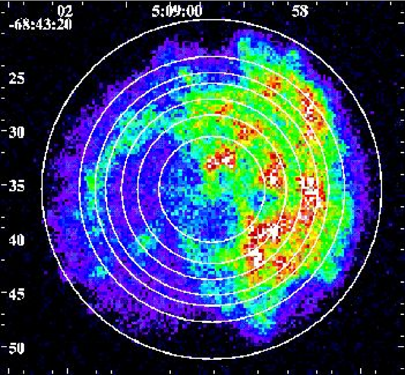
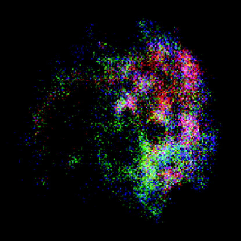
Figure 2: Top -- Intensity map of N103B, using a linear scaling, ranging from 0 (black) -- 75 (white) counts pix^-1. The annular regions to be analyzed in §3.3.1 are indicated with solid rings. Bottom -- An X-ray color image of N103B with red (0.5 -- 0.9 keV), green (0.9 -- 1.2 keV) and blue (1.2 -- 10.0 keV). The bin size in both images is 0.5^′′.

The spectrum extracted from the entire remnant is very similar to the ASCA spectrum (Hughes et al., 1995), showing strong K$\alpha$ lines of Si, S, Ar, Ca, and Fe and soft X-ray emission ($\sim 1$ keV) dominated by emission from Fe L-shell transitions (Figure 1). The Fe K$\alpha$ line at $\sim$6.4 keV is much more significant in the Chandra spectrum, as the ASCA spectrum was contaminated by background at high energies (Hughes et al., 1995). In Figure 2 (Top), we show the 0.4-8 keV image of N103B obtained with Chandra. This image reveals significant structure at the arc-second level and the bright western half of the remnant is now resolved as a series of dense knots as well as diffuse emission. An X-ray color image composed from red (0.5 -- 0.9 keV), green (0.9 -- 1.2 keV) and blue (1.2 -- 10 keV), shown in Figure 2 (Bottom), further reveals that the spectral characteristics vary throughout the remnant as well. On large scales, the emission in the northwest is softer than the emission from the south. The color varies slightly from one knot to the next, showing that the spectral variability extends to small scales as well.

3.2 Narrow Band Imaging

To gain insight into the distribution of Si and S throughout the remnant, we produced continuum-subtracted (CS) and equivalent-width (EW) images following the methods outlined by Hwang, Holt, & Petre (2000). To do this, images were extracted from the energy interval of the Si and S emission lines as well as two continuum regions straddling each of these lines. The energy intervals and image properties used for each image are listed in Table 1.

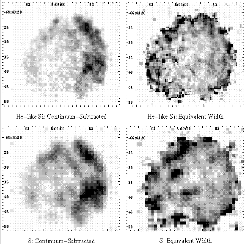
Figure 3: Continuum-Subtracted (left) and Equivalent Width (right) images of N103B in He-like Si and S. All images are plotted with a linear scale ranging from 0 (white) -- 10 counts pix^-1 (subtracted images) and 0 (white) -- 1 keV (EW images). The bin size and smoothing size for each image is listed in Table 1.

After smoothing each image with a boxcar, a linear interpolation between the two continuum images was performed pixel by pixel to create an image of the continuum contained in the energy interval of the emission line. We neglected any spectral variations within the two continuum bands, since they are negligible compared to the variations between the bands. The CS image was produced by subtracting this continuum image from the original line image. To create the EW image, the CS image was divided by the continuum and then this ratio was normalized by the width of the energy interval (in units of keV) to obtain the EW image. As can be seen in Figure 3, the CS images for He-like Si and S are strikingly similar to the 0.4 -- 8 keV image (Fig. 2, Top), showing bright knots throughout the western half of the remnant. Underlying radial trends in the remnant are clearly revealed in the EW map, however.

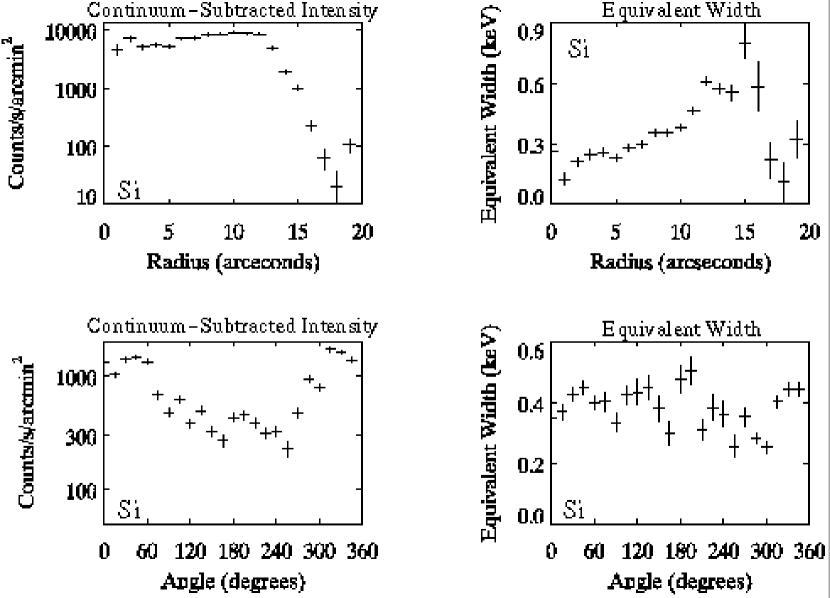
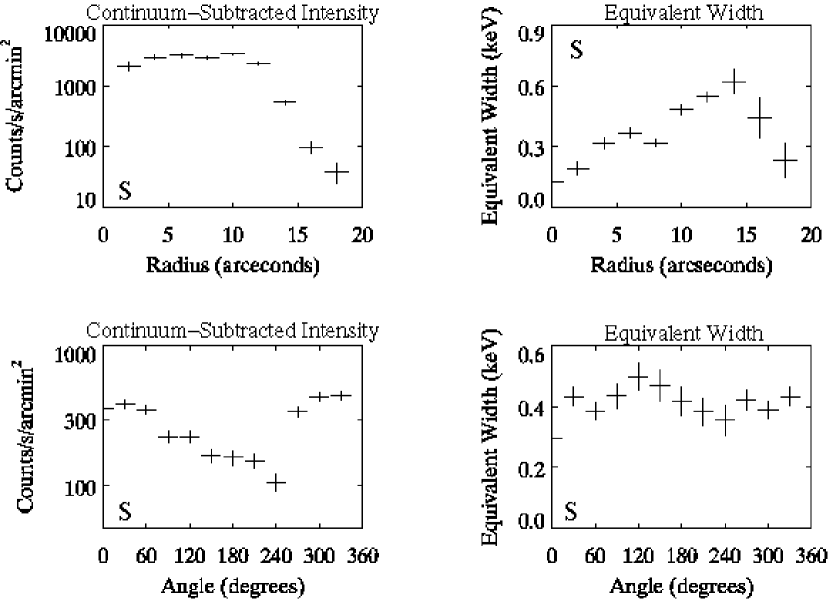
Figure 4: The dependence of the Continuum-Subtracted Intensity (left) and Equivalent Width (right) upon radius and angle for He-like Si (top two panels) and S (bottom two panels). 0^o is West.

It is apparent from the He-like Si and S EW images that the strength of these lines (as compared to the continuum) increases significantly along the rim of the remnant. To determine whether the emergence of the ring-like structure is an artifact of the low count rate in the rim, the original line and continuum images were collapsed into the radial and azimuthal dimensions by binning the images into rings and sectors. The CS intensity and EW were calculated for each bin, this time employing a logarithmic interpolation between the continuum regions, which is more suitable for the spectrum of N103B (see Figure 1). The radial and azimuthal plots, shown in Figure 4, confirm what is seen in both the CS and EW images (Figure 3). The CS intensity peaks at a radius of $\sim 10^{\prime\prime}$ with a strong azimuthal dependence. By contrast, the EW plots show little azimuthal dependence. Most importantly, there is a clear increase in the equivalent width with radius beginning at a radius of $\sim 10^{\prime\prime}$ and peaking at $\sim 15^{\prime\prime}$, which is the rim of the remnant.

The Si and S EW images reveal an extremely simple radial structure, in contrast to the spatial and spectral complexity revealed by the false-color and X-ray color images. A detailed study of the these radial variations present an excellent way to study the spatial distribution of the ejecta. Thus, in the following sections, we focus solely on the radial variations and leave an analysis of the intriguing small-scale structure seen in the X-ray color image to future work.

3.3 Spectral Modeling

To study the radial variations in more detail, we divided the remnant into 7 concentric rings, each with $\sim 35,000$ counts. The extraction region for each ring is listed in Table 2 and shown in Figure 2 (Top). The equivalent width (EW) of the emission lines depends both upon the total number of emitting atoms which are present as well as the temperature and ionization state of the atoms. To determine the cause for the variations in the EW, it is necessary to perform detailed spectral modeling to determine which of these factors are contributing.

3.3.1 The Spectral Model

We use a plane-parallel shock, non-equilibrium ionization (NEI) model (Hughes, Rakowski, & Decourchelle, 2000), which has been incorporated into the XSPEC v. 11.0.1 analysis package. This model uses a single temperature, T, but includes a range of ionization timescales, integrated from 0 to n_et s cm^-3, where n_e is the electron density and t is the time elapsed since the material was heated to a temperature T. This NEI model allows for each element to have independent temperatures and ionization states which can be linked as desired. We use two absorbing columns, using the cross-sections of Balucinska-Church & McCammon (1992): one to account for galactic absorption (frozen at $7\cdot 10^{20}$ cm^-2; Dickey & Lockman 1990) and the other, with lowered abundances, to model the absorption within the LMC (allowed to vary to obtain the best fit). The abundances of the LMC column are fixed at the values derived from the optical studies of H II regions and evolved supernova remnants in the LMC by Russell & Dopita (1992) and X-ray studies of evolved supernova remnants by Hughes, Hayashi, & Koyama (1998). When neither study provided a measurement, the abundance of that element was set to 0.3, relative to solar, which is the average abundance in the LMC. Throughout, the solar abundance pattern of Anders & Grevesse (1989) is used. The assumed values are given in Table 3. Finally, a narrow Gaussian component at $\sim 0.7$ keV is added to all the spectra to fill in a deficit in the modeled spectrum at the energy. A similar deficit is noted by Hwang, Hughes, & Petre (1998) in the analysis of several SNRs using an earlier version of this NEI code. Thus we believe that a line or line-blend is missing from the model, and the deficit does not indicate a serious flaw in the derived model parameters.

We find that it is impossible to fit the spectra with a single NEI plasma model for all elemental species; it is necessary to include several thermodynamic components to adequately model the data. The bulk of the continuum emission arises from a $\sim$ 1 keV plasma, which we model as hydrogen (although any featureless continuum would suffice as well). Emission from Si, S, Ar, Ca, Fe also arises from a $\sim$ 1 keV plasma with a large ionization timescale (n_et$>10^{12}$ s cm^-3). In all the spectra, the strength of the Fe K-$\alpha$ emission line is under-predicted by this single temperature model. Following the results of Hwang, Hughes, & Petre (1998), we allow for additional Fe in a high temperature ($>2$ keV) plasma which has a low ionization timescale (n_et$<$10¹¹ s cm^-3). Finally, the H-like Mg emission line is too weak, relative to the He-like line, to arise from the same high ionization timescale plasma as the Si. Thus we include O, Ne, and Mg emission in a third lower-ionization timescale (n_et $\sim 10^{11}$ s cm^-3) component. The temperature of this component is poorly constrained, but is generally consistent with 1 keV. Although Ne and O lines are not explicitly seen in the $ACIS$ spectrum, they are seen in $XMM-Newton$ RGS (van der Heyden et al., 2002) and $Chandra$ LETG (Migliazzo et al., 2002) grating observations. In our data the O and Ne lines are blended with the many emission lines from L-shell transitions of Ar, Ca, and Fe, so it is not surprising that clear O and Ne emission lines are not seen. We add O and Ne to the lower-ionization timescale component, as O and Ne are produced in the O-burning zone along with Mg, as discussed in Sec. 4.1. Throughout, we refer to the components as the ‘‘H’’, ‘‘Si’’,‘‘Hot Fe’’, and ‘‘O’’ components.

We do not account for any emission from Co and Ni. The bulk of the radioactive Co and Ni produced in the initial explosion will have decayed already, although some non-radioactive isotopes may to be present. Furthermore, the L-shell emission of these lines overlap with those of Fe and no K$\alpha$ lines are evident, making it difficult to constrain the abundances of these elements. Finally, it is not necessary to include a blastwave component at a separate temperature to model these data. A swept-up ISM component may be related to the 1 keV hydrogen plasma that we require in our fits.

3.3.2 Spectral Analysis Results

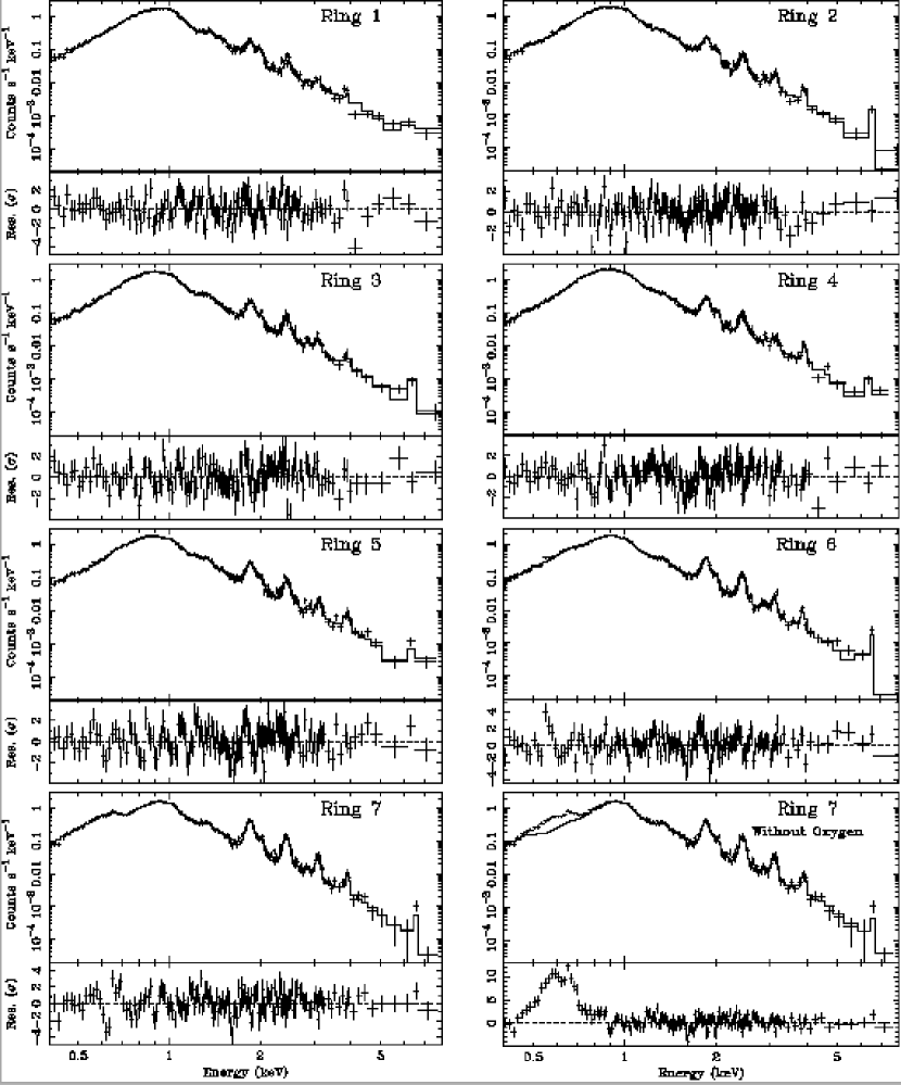
Figure 5: The first seven panels show the spectrum from each of the seven extraction regions along with the best fit using the four-component NEI model. The fit parameters are shown in Tables 4 and 5. The eighth panel (lower right corner) shows the effect of removing the oxygen emission from the best fit model for Ring 7. As seen in the residuals, the oxygen emission is quite strong, despite the lack of a clear emission line in the spectrum. The upper portion of each panel shows the data and the model (solid line) while the bottom portion shows the residuals, normalized to the standard deviation, $\sigma$.

The spectral fits are shown in Figure 5 and the model parameters are listed, with 90% errors, in Tables 4 and 5. These errors were obtained by stepping through each parameter to determine the change in the $\chi^{2}$. The true errors on the quantities may be larger, since this method assumes that the best-fit model is correct and does not incorporate the systematic uncertainties which may be introduced by the chosen model. Furthermore, the error bars on quantities which are dependent upon each other, such as temperature and ionization, may be larger than estimated since these parameters were not varied in pairs. Also included in Figure 5 (lower right corner) is a plot of the spectrum and model for Ring 7 in which the oxygen emission has been omitted; clearly, oxygen is required to fit the data, although the emission line is not resolved. We leave a detailed discussion of the quality of model fits to the end of this section and here briefly present the results of the spectral fits, which will be discussed in more detail in the §4.

In Table 4, we list the best fit temperatures and ionization states for the O, Si, and Hot Fe components. The temperature of the H component is identical to the Si temperature, within error bars, and is not listed. In general, the temperature and ionization timescale within each component remain fairly constant with radius. We note that the LMC column density decreases greatly in the outermost ring. It is difficult to determine whether this decrease takes place throughout the entire ring, as the soft emission from the north-west (Fig. 2 Bottom) contributes a large fraction of the total emission in the outermost ring.

In Table 5, we present the volume emission measure (EM) of each element, given by $n_{\rm e}n_{\rm i}V/4\pi D^{2}$, where $n_{\rm e}$ and $n_{\rm i}$ are densities of the electrons and ions, respectively, $V$ is the volume of the emitting region, and $D$ is the distance to the remnant. Within the O and Si components we report the EMs of the other elements in the component relative to either the O or Si EM. If the emission from each species within a single component arises from the same volume, then the ratio of two EMs within a component is simply a ratio of the ion densities of the two elements, which in turn is related to their abundances and masses. As described in the previous section, the O, Ne, and Mg emission lines are not clearly resolved and the EMs associated with this component should be treated with caution.

There are several striking trends in the EMs reported in Table 5. First, the EM of Si rises steadily from Ring 1 to Ring 7, mimicking the behavior of the equivalent width of He-like Si shown in Fig. 4, while the EM of the hot Fe declines (See Fig 6). Second, the EMs of S, Ar, Ca, and Fe, relative to Si, are roughly constant within the error bars. An exception is the highly elevated Fe EM in Ring 1. Third, neither the H nor O EM show any clear radial trend and they vary in concert, with the O EM being 2$\cdot 10^{-5}$ times the H EM, within errors. Although the Ne and Mg EMs, relative to O, are not constant within error bars, they also do not show any clear radial trend.

From this spectral analysis, it is clear that the increase in the equivalent widths of Si and S with radius seen in the narrow band images (Figs. 3 and 4) is not due to a change in the temperature or ionization state of the Si and S emitting plasma, but an increase in the EM of the Si component. Since the temperature, ionization, and composition of the Si component are roughly the same in the seven extraction regions, the only way to increase the EM is by increasing either the ion density or the volume of the Si component contained in the outer extraction regions. In either case, the variations in the EM trace the physical distribution of the Si component, and can be a powerful tool for studying the morphology of this emission component. Similarly, the distribution of the hot Fe component is also traced by its EM. In §4.2, we model the variations in the EMs of the hot Fe and Si components in detail to place constraints on the three-dimensional distribution of the material in these two components.

Finally, we note that the densities of S, Ar, and Ca, relative to Si, are elevated above those expected from the LMC (Table 3), while the relative density of the Fe in the Si component is considerably lower than expected from the LMC. Although some ISM may have been swept up, it is clear that the emission in the Si component arises primarily from ejecta. The hot Fe is naturally assumed to also be a component of the ejecta. However, the densities of Ne and Mg, relative to O, are significantly higher than expected from the LMC (0.18 and 0.054, Table 3) or either a Type Ia (0.014 and 0.059) or Type II (0.11 and 0.069) SNR (Iwamoto et al., 1999; Tsujimoto et al., 1995). It is not entirely clear whether the O, Ne, and Mg emission arise from ejecta or the swept-up material. In §4.3 and §4.4, we will study the EMs in detail to investigate the origin of the various emission components.

3.3.3 Discussion of the Spectral Fits

The model fit in all seven rings is generally quite good across the entire 0.4-8 keV range. Here we discuss several sources of the residuals and their impact upon the fit parameters.

Although the CTI correction compensates for gain variations across the detector, minor errors ($\leq 1\%$) in the gain are expected to remain (Townsley et al., 2001a). This is particularly true for data obtained at a focal plane temperature of -110^o as there is a limited data-base of calibration data with which to tune the CTI corrector. We noticed slight systematic shifts in the energy centroids of the strong K-shell Si, S, Ar and Ca emission lines, which become progressively worse in the outer rings. While these shift are not large, the data are of sufficient quality that they affect the $\chi^{2}$ of the fit dramatically Further, the emission measures of the elements would be somewhat underfit, compromising our analysis of the ejecta distribution. Thus, in our fits we applied a slight adjustment to the gain ($<1\%$), by including the slope of the gain as an additional fit parameter. Some slight offsets are still visible in the residuals, but these are not significant.

The residuals in the fit to the spectrum of Ring 7 are considerably larger than seen in the other rings. The spectra of the eastern and western halves of this ring are quite different below 1 keV, which makes it difficult to fit the combined spectrum. The spectrum of the eastern half of Ring 7 is quite similar to those of the inner six rings while the spectrum of the western half exhibits the 0.7 keV deficit seen in the combined spectrum (Fig. 5). The quality of the spectral fit to the eastern half of Ring 7 is quite good ($\chi^{2}_{\nu}=1.3$) with fit parameters, particularly the emission measures, similar to those derived from the fit to Ring 7 as a whole, although with larger error bars due to the greatly reduced count rate. Thus we are confident that, despite the statistically poorer fit to Ring 7 as a whole, the derived fit parameters are reliable.

4 DISCUSSION - ORIGIN AND DISTRIBUTION OF THE EJECTA

In the previous section, we demonstrated that N103B contains a large amount of hot Fe with a low ionization timescale, similar to that found in Tycho’s SNR (Hwang, Hughes, & Petre, 1998). As shown by the radial variations in the emission measure (EM), this hot Fe component is located centrally, as seen in Tycho’s SNR (Hwang & Gotthelf, 1997), while the Si component, composed of Si, S, Ar, Ca, and additional Fe, is more prominent in exterior regions of the remnant. Qualitatively, the distribution of the elements is more similar to that inferred for Tycho’s SNR than that seen in Cas A and G292.0+1.8. With this in mind, we compare the properties of N103B with remnants of Type Ia SNe.

To aid the following discussion, we begin with a brief overview of nucleosynthesis models in Type Ia SNe and the predicted distribution of the ejecta. Then in §4.2, we model the variations in the Si and hot Fe EMs in detail, taking into account the 3D structure, to place constraints upon the distribution of the ejecta. In §4.3, we discuss the origin of the hot Fe component and in §4.4 briefly discuss the H and O components. Finally, in §4.5, we calculate the masses of the ejecta and compare with the expected masses of the ejecta produced in Type Ia and Type II SNe.

4.1 Overview of Nucleosynthesis in Type Ia SNe

Iwamoto et al. (1999) model the nucleosynthesis in Chandrasehkar mass models for Type Ia SNe. The authors consider pure deflagration models (of varying deflagration speed) as well as delayed detonation models in which the deflagration front transitions to a detonation front. Here we describe the fast deflagration W7 model (Nomoto, Thielemann, & Yokoi, 1984; Iwamoto et al., 1999). Complete Si burning occurs in the inner $\sim 0.8~{}\rm M_{\odot}$ of the white dwarf, producing the Fe-peak nuclei: Ni, Fe, and Co. The central core ($\sim 0.2~{}\rm M_{\odot}$) is primarily non-radioactive ⁵⁶Fe and ⁵⁴Fe, but ⁵⁶Ni is the dominant species produced throughout the rest of the Si-burning zone. Incomplete Si burning (from $0.8-1.2~{}\rm M_{\odot}$) leaves behind ⁵⁴Fe, Ca, Ar, S, and Si. Finally, in the outer $\sim 0.2~{}\rm M_{\odot}$ O, Ne, and C are burned, leaving behind additional Si as well as Mg, Ne, and O. The transition from one burning zone to the next is rather sharp and the overlap between complete and incomplete Si burning products is quite small. The delayed detonation models produce a qualitatively similar distribution, but the transition between the complete and incomplete Si-burning zones is blurred and the Fe-peak nuclei and Si-burning products can co-exist throughout a large fraction of the remnant.

4.2 3D Distribution of the Ejecta

In §3.3.2, we concluded that the EMs in the Si and hot Fe components change either because the ion density or volume changed from one extraction region to the next. In principle, one could assume that all seven extraction regions contained an identical volume of ejecta from both components and that the ion densities varied from one region to the next. However, it is more physically reasonable to explain the EM variations with changes in the volume.

As suggested by the models for Type Ia SN nucleosynthesis presented above, in the absence of mixing, the ejecta of a SNR are expected to be radially stratified with Fe-rich core surrounded by a Si-rich shell. Although each of the seven extraction regions we have chosen will include emission from both the Fe core and Si shell, an interior extraction region will contain a larger volume of the Fe core than an exterior extraction region, while the opposite holds for the Si shell. Qualitatively, one can easily account for the variations in the Si and hot Fe emission measures by this simple geometrical effect.

To place constraints upon the 3D distribution of the ejecta, we begin by modeling the ejecta as a spherical volume with three zones. An outer shell is filled by the Si component and hot Fe is located in a shell interior to this. To account for the enhancement of Fe in Ring 1, we include a small sphere of Fe in the center of the remnant. This is also consistent with the slight decrease in the hot Fe EM in Ring 1, as the volume of the hot Fe zone contained in the Ring 1 is reduced (Table 5 and Fig. 6). The inner sphere of Fe may be associated with the core of ⁵⁴Fe and ⁵⁶Fe. Within each zone, the density is assumed to be constant. The transition radii between the zones are given by $\rho_{1}$ and $\rho_{2}$, where $\rho$ is normalized by 16^′′, which is the projected radius of the outermost extraction region.

From this 3D model, we predict the EMs that would be observed by determining the volume of each of the three zones which is contained in a particular extraction region, given the assumed $\rho_{1}$ and $\rho_{2}$. The volume of a sphere contained in a 2D annular extraction region is given by:

$$V=4\pi\int_{{\rm R}_{1}}^{{\rm R}_{2}}\rm{RdR}\int_{\sqrt{\rho^{2}-{\rm R}_{1}^{2}}}^{\sqrt{\rho^{2}-{\rm R}_{2}^{2}}}dz=\frac{4}{3}\pi((\rho-{\rm R}_{1}^{2})^{3/2}-(\rho-{\rm R}_{2}^{2})^{3/2}),$$

where R and z are the cylindrical coordinates, $\rho$ is the radius of the sphere, and R₁ and R₂ are the inner and outer radii of the annular extraction region. Given the inner and outer radius of each of the three zones, $\rho_{1}$ and $\rho_{2}$, it is possible to determine the volume of each zone which is contained in a particular extraction region.

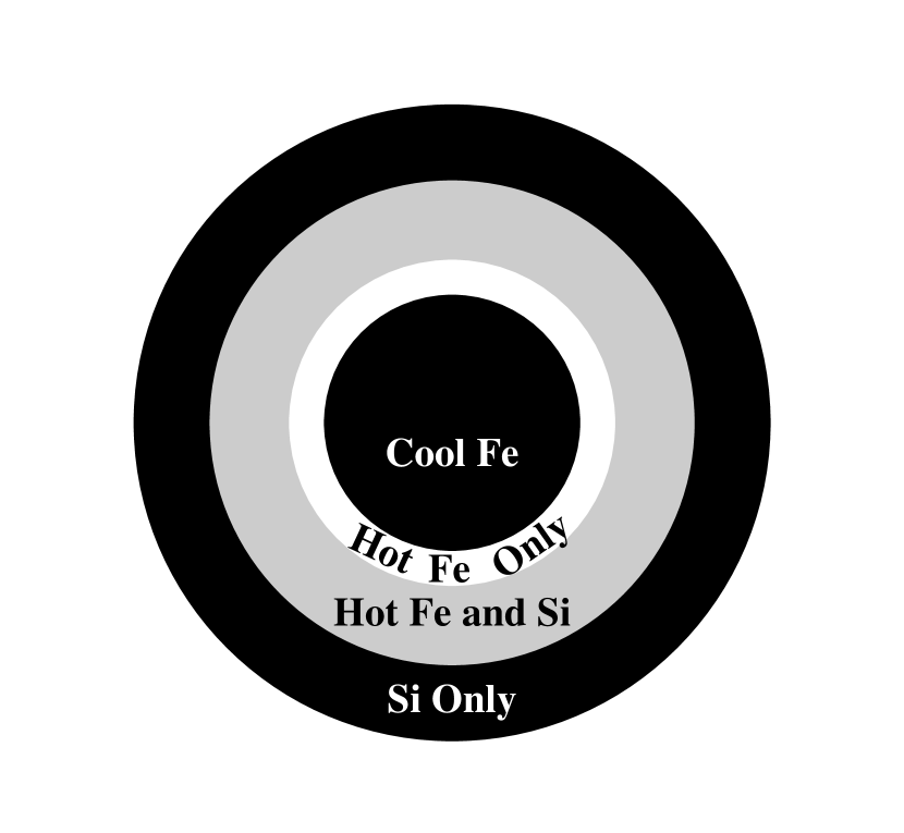
Figure 7: Model cross-section of N103B, based upon the three-zone model developed in §4.2 and the fit parameters found in Table 6.

In each extraction region, EM_obs = $K\cdot V_{\rm zone}/V_{\rm tot}$, where EM_obs is the measured EM (Table 5), $V_{\rm zone}$ is the calculated volume of the zone which is contained in the extraction region, and $V_{\rm tot}$ is the total volume of the remnant. In terms of physical quantities, $K$ = $n_{\rm e}n_{\rm i}V_{\rm tot}/4\pi D^{2}$ cm^-5. The Si and hot Fe EMs were fit separately by stepping through a range of $\rho_{1}$, $\rho_{2}$, and $K$ to map out a 3D $\chi^{2}$ space to locate the minimum. When fitting the Si EM, $\rho_{1}$ is set to 0, since changes in this parameter do not affect the Si EM. The fit parameters are shown in Table 6 and the best fits are plotted in Fig. 6. Although the fits are statistically unacceptable, the qualitative agreement between the observed data and the predictions of this simple model is remarkable. In Fig. 7, we show a schematic diagram of the three-zone model for N103B.

Although this model assumes that the hot Fe and Si zones do not mix, it is clear from the different fit values of $\rho_{2}$ (Table 6) that there must be a large region of overlap between the two zones. As a result, the masses obtained in §4.5 will be somewhat overestimated, because we assume throughout that each component completely fills the volume of its zone. The large overlap between the hot Fe and Si components could indicate that the distribution may be more similar to that predicted by the delayed detonation models (See §4.1). However, significant mixing between these two layers could occur at a later time, and we cannot rule out a fast deflagration model for this remnant.

4.3 Origin of the Hot Fe

We have found that the Fe K-shell and a large fraction of the Fe L-shell emission arises from a hot ($>2$ keV), low ionization timescale (n_et$\sim$10^10.8 s cm^-3) plasma. Although the hot Fe is located in the interior, it overlaps spatially with the Si component. It would be very difficult to shock the hot Fe at a significantly later time than the Si component, as suggested for Tycho’s SNR (Hwang, Hughes, & Petre, 1998). Alternatively, the electron density in the hot Fe component could be much lower than in the Si component, leading to a low ionization timescale.

In their analysis of SN 1987A, Li, McCray, & Sunyaev (1993) find that $\sim 10$% of the energy released in the radioactive decay sequence $\rm{{}^{56}Ni(e^{+},\gamma)^{56}Co(e^{+},\gamma)^{56}Fe}$ is absorbed locally. As a result, clumps of Ni/Co/Fe are heated to a much higher temperature than the rest of the plasma. These clumps expand until they come into pressure equilibrium with the surrounding plasma. It is estimated these bubbles have a filling factor of 30$\%$ in SN 1987A. While the hot, low density bubbles initially include Ni, Fe, and Co, the bubbles will eventually be composed primarily of ⁵⁶Fe. The low density of the bubbles leads naturally to a lower ionization timescale.

Blondin, Borkowski, & Reynolds (2001) model the dynamics of these Fe bubbles. As the reverse shock passes through the bubbles, the postshock temperature is significantly higher, due to the low density of the bubbles. Additionally, they find that the presence of Fe bubbles leads to vigorous mixing, which will destroy the initial radial structure of the remnant; a distinct shell of ejecta are not expected. Large variations in pressure and temperature are expected as well. They further find that as the bubbles expand into the surrounding material, the ejecta are compressed into narrow, dense filaments which partially trace out the boundaries of the Fe bubbles. It is expected that 90% of the emission measure in the SNR may arise from less than 2% of the volume of the shocked gas.

Wang & Chavalier (2001) consider the effects of Fe bubbles in the specific case of a Type Ia remnant with an exponential density profile which is expanding into a constant density medium. This study was motivated, in part, by observations of Tycho’s SNR, which indicate the existence of ejecta at very large radii (Hwang & Gotthelf, 1997) as well as two nearly undecelerated knots of ejecta (Hughes, 1997). They suggest that the ejecta at large radii are primarily in the form of dense clumps which decelerated less rapidly than the surrounding ejecta. To exist so close to the boundary of the shock, the knots must be $\sim$ 100 denser than the surrounding medium. This high compression factor is not a natural consequence of Rayleigh-Taylor instabilities and Wang & Chavalier (2001) argue that Fe bubbles are necessary to create such dense clumps of ejecta. Since the hot Fe bubbles and the other ejecta are expected to be shocked at the same time, the ionization timescale for the hot Fe is expected to be $\sim$ 100 smaller than for the other ejecta.

The Fe bubbles are an attractive explanation for the hot Fe seen in this remnant for several reasons. The location of the hot Fe component, as shown in Fig. 6 is consistent with the expected distribution of ⁵⁶Ni, as described in §4.1. Furthermore, the Fe component has an ionization timescale which is $\sim$ 100 times lower than that of the Si component. Morphologically, N103B has a filamentary structure, particularly on the western side of the remnant (Fig. 2, Top) and as in Tycho’s SNR, there is a large amount of ejecta at relatively large radii (Fig. 4). However, the mixing in N103B does not appear to be as severe as predicted by the hydrodynamical simulations of Blondin, Borkowski, & Reynolds (2001) and Wang & Chavalier (2001).

4.4 The Hydrogen and Oxygen Components

Before beginning a discussion of the H and O components, it is important to note that the EMs of O, Ne, and Mg should be treated with caution, since there are no strong, isolated, emission lines from these species observed in our spectrum (See §3.3.1). Thus, any conclusions drawn here should be viewed with some caution.

While the EMs of the H and O components vary quite a bit from one ring to the next, there is no clear radial trend, as is seen in the Si and hot Fe components. The H and O components vary in concert, with the O EM $\sim 2\cdot 10^{-5}$ times the H EM and the EMs of both components $\sim$ 50% larger in the rings in which the bright clumps occupy a large projected area of the extraction region. This strongly suggests that the H and O components must be physically connected. The lack of radial variations and the sharp drop in emissivity beyond 16^′′ suggests that the H and O components are not in a shell surrounding the remnant, but are found in a clumpy foreground or background structure in the ISM which has interacted with the remnant and been heated to X-ray emitting temperatures.

However, the number density of O, relative to H, is an order of magnitude smaller than expected from material in the LMC. This problem would be resolved if the O component were linked with only a portion of the H component, but then it would be difficult for the two components to fluctuate simultaneously by 50%. On the other hand, the Ne and Mg number densities, relative to O, are much higher than expected from the ISM.

One could argue that the O component is composed of ejecta. However, in this case, it is very difficult to understand the intimate relationship between the H and O components and the lack of radial variations in the O EM. Furthermore, the number densities of Ne and Mg, relative to O, are also higher than expected for both Type Ia and Type II SNRs.

Using the radial variations alone, very little can be said about the origin or distribution of the H and O components. Spectroscopy of the bright clumps may give more insight into these questions. It is clear, though, that the H and O components do not occupy the same physical space as the Si component. Therefore, the abundances and EMs of the species in the O and Si component should be compared with extreme caution.

4.5 Masses of the Ejecta

Using the emission measures (EMs) listed in Table 5 and the 3D model of the ejecta distribution found in §4.2, the mass of each element can be estimated. Recall that the normalization factor used in the 3D model is $K=n_{\rm e}n_{\rm i}V_{\rm tot}$/4$\pi D^{2}$ cm^-5, where $V_{\rm tot}$ is the total volume of the remnant.

Within the Si component, the electron density, $n_{\rm e}/n_{\rm Si}$, is given by the sum over all species of $n_{i}/n_{\rm Si}X_{i}\cdot Z_{i}$, with $i$ ranging from Si to Fe. We obtain $n_{i}/n_{\rm Si}$ directly from Table 5, $X_{i}$ is the ionization fraction calculated within the NEI code, and $Z_{i}$ is the charge of each species. We averaged the values of $n_{i}/n_{\rm Si}$ for S, Ar, and Ca from all seven rings, but excluded the first ring when calculating $n_{\rm Fe}/n_{\rm Si}$. Using this information, we obtained $n_{\rm e}/n_{\rm Si}$ = 39. Since the extraction region of Ring 7 extends to 16^′′, or 3.9 pc, we use this as the boundary of the total emitting volume. Using $D$ = 50 kpc, we obtain $n_{\rm Si}=1.4\cdot 10^{-3}{\rm cm}^{-3}$. If we assume that the Si component completely fills the Si zone ($\rho$ = 0.51--1.0), then we obtain a Si mass of 0.21M_⊙. Using the average $n_{i}/n_{\rm Si}$ used above, we obtain the masses of all the elements in the Si component, which are listed in Table 7.

Similarly, in the hot Fe component, $n_{\rm e}/n_{\rm hot\,\rm Fe}$ = 19 and $n_{\rm hot\,\rm Fe}=1.6\cdot 10^{-3}{\rm cm}^{-3}$. Assuming that the hot Fe component fills the region $\rho$ = 0.4 -- 0.77, we obtain 0.21M_⊙ of hot Fe. Finally, to estimate the mass in the Fe core, we use the excess Fe EM in Ring 1, which is 3.9$\cdot 10^{6}$ cm^-5. We also note since there is an Fe enhancement only in Ring 1, the Fe core probably does not exceed $\rho=0.32$. In this zone, $n_{\rm e}/n_{\rm Fe}$ = 21, leading to $n_{\rm Fe}=5.1\cdot 10^{-3}{\rm cm}^{-3}$ and a Fe core mass of 0.06 M_⊙. From all three zones, we have a combined Fe mass of 0.34 M_⊙. It is impossible to calculate the masses in the H and O components because we have no estimate of the emitting volume.

The masses calculated above could be over- or underestimated for several reasons. First, we note that the estimated electron density in the Si component is not even twice that in the Fe component. If we wish to rely only upon a difference in electron density to account for the difference in ionization timescale, the Si component will need to be in the form of dense clumps with a very small filling factor. This is not inconsistent with the simulations performed by (Blondin, Borkowski, & Reynolds, 2001) (Wang & Chavalier, 2001). However, if the Si component is highly clumped, the masses from this component will be significantly reduced. Second, the assumption of a pure metal plasma results in a larger mass than if we had assumed a highly enriched but still H/He dominated plasma. This is particularly relevant in the Si component, as it is possible that some ISM has been swept up into this outer shell. Finally, we cannot assume that all of the ejecta are visible in X-rays. Since the remnant is not center-filled, it is possible that the ejecta in the interior have not been completely shocked by the reverse front. Thus the mass of the Fe ejecta in particular may be considerably higher than estimated above.

Given these considerations, the estimated masses of Si, S, Ar, Ca, and Fe are in better agreement with the predictions of a Type Ia (W7) model than a core-collapse SN (Table 7). Additionally, the O-rich component of N103B appears to be associated with a structure in the ISM, rather than an O-rich zone of ejecta one would expect from a core-collapse SN.

5 CONCLUSIONS AND SUGGESTIONS FOR FUTURE WORK

The spectrum of N103B obtained through this Chandra observation is quite similar to the ASCA spectrum (Hughes et al., 1995), showing strong K$\alpha$ lines of Si,S, Ar, Ca and Fe, suggesting a Type Ia origin for the remnant. The Chandra image of N103B reveals structure at the sub-arcsecond level. The bright western side of the remnant, seen in previous X-ray images, is composed of a series of bright knots and filaments. An X-ray color image reveals that the spectral characteristics also vary dramatically throughout the remnant.

We find that despite the complex spatial and spectral morphology suggested by the false-color and X-ray color images, there are striking radial trends in the equivalent widths of the strong Si and S emission lines, as revealed by narrow band imaging. The equivalent widths remain fairly constant within the interior, then rise rapidly at a radius of 10^′′. To investigate the cause for the increase in equivalent width through spatially resolved spectroscopy, we divided the remnant into seven concentric rings, each with approximately 35,000 counts.

The data are well fit by a plane-parallel, non-equilibrium ionization model. The continuum emission arises primarily from a 1 keV hydrogen plasma. An additional $\sim$ 1 keV plasma with a high ionization timescale (n_et$>10^{12}$ s cm^-3) contains Si, S, Ar, Ca, and Fe. A hot ($>2$ keV), low ionization (n_et$\sim$10^10.8 s cm^-3) Fe plasma is required to produce the strong Fe K$\alpha$ line. Finally, the O, Ne, and Mg are located in a plasma with an ionization timescale of n_et$\sim$10¹¹ s cm^-3 and temperature of roughly $\sim$ 1 keV. The components are referred to as the H, Si, hot Fe, and O components, respectively.

Using this spectral model, we have determined that there are no significant radial variations in the temperatures or ionization timescales of the components. Instead, we find that the emission measures (EM = $n_{e}n_{i}V/4\pi D^{2}$) of the species in the Si component increase radially, mimicking the radial profiles of the Si and S equivalent width images. An exception is an enhancement of Fe in the innermost extraction region. In contrast to the Si component, the hot Fe EM has a profile which drops rapidly at radii greater than 10^′′.

The EM variations in the Si and hot Fe components are well modeled by a simple three-zone model for the ejecta. In the interior of the remnant is a sphere of Fe with a temperature of 1 keV and a high ionization timescale, which occupies only the inner 3% of the remnant’s volume. Exterior to this is a shell of hot Fe which is plausibly in the form of hot Fe bubbles. Finally, surrounding the hot Fe is a shell of Si, S, Ar, Ca, and Fe. The Si and hot Fe components coexist for a large fraction of the remnant volume, implying that the difference in ionization timescale, $n_{e}$t, is due to a difference in electron density.

We have limited information about the location and origin of the H and O components. The EMs of these components show no radial trends, like those seen in the Si component. Furthermore, these components vary in concert, suggesting that the two components are physically linked. It is likely that these two components are associated with a clumpy foreground or background structure in the ISM which has been shocked by the remnant, rather than a shell of ejecta or swept-up material. It is clear that the O component does not occupy the same volume as the Si component, and that any comparison between these two components must be performed with care. In particular global O, Si, and Fe abundances derived from integrated spectra of this remnant cannot be directly compared to nucleosynthesis models without first taking into account the different physical locations of the different components.

Finally, we estimate the masses of Si, S, Ar, Ca, and Fe and find that they are more consistent with the yields of a Type Ia SN than a Type II SN. In particular, the large mass of Fe (0.34 M_⊙) suggests that a Type Ia origin for N103B is more likely. Further support for a Type Ia origin is the lack of an O-rich component of ejecta. Finally, the properties of N103B are strikingly similar to Tycho’s remnant. Both require a hot Fe component and show a radial segregation of the Fe and Si components of the ejecta. The results of this analysis indicate that the properties of N103B are consistent with a Type Ia origin. However, further work must be done, particularly to determine the location and origin of the O component, before eliminating a Type II origin.

Certainly, a more realistic 3D model of the ejecta is needed, which takes into account the initial structure of the remnant, the expansion, and potentially mixing between the layers. Additionally, throughout this paper, we have ignored the large asymmetry between the eastern and western halves of the remnant; to model this remnant more accurately, this must be taken into account. Using more sophisticated models for seven radial bins is pointless however, and we suggest that the analysis be improved by combining this ACIS dataset with the 0^th order Chandra LETG grating data. With this larger dataset, the remnant could be sampled with finer radial bins and the differences between the eastern and western halves could be explored. Also, by using the information from the Chandra and XMM-Newton gratings observations, one could restrict the parameters of the O component more effectively, thereby reducing some of the uncertainties in this analysis.

Finally, this analysis has ignored the intriguing small-scale variations in brightness and color. An exploration of these may yield more clues to the origin and distribution of the O and H components. In particular, it important to determine whether these clumps have the same composition as the rest of the remnant, or whether they are dominated by emission lines or continuum. Again, while several of the brighter clumps have 10,000 counts, the model we have proposed cannot be safely used unless a strong Fe K$\alpha$ line is present to remove some of the confusion between the two different sources of Fe emission. Again, combining the 0^th order Chandra LETG grating and ACIS datasets should improve matters greatly.

Figure 1: The integrated spectrum for N103B. The spectrum has been binned so that a minimum of 25 counts are in each energy bin. The K$\alpha$ and K$\beta$ lines of highly ionized Mg, Si, S, Ar, Ca and Fe are labeled.

Figure 6: Plot of the Si and hot Fe emission measures (EMs) as a function of radius. The data points and error bars represent the fit values, shown in Table 5, while the lines connect the predicted EM for each ring, calculated using the simple 3D model for the ejecta discussed in §4.2. The sudden increase in both the measured and predicted EMs in Ring 4 is due to the slightly larger volume contained in Ring 4, as compared to Rings 3 and 5.

Table 1:

	He-like Si	S (He- & H-like)
Line (eV)	1750:1915	2340:2540
Left Cont. (eV)	1565:1730	2120:2320
Right Cont. (eV)	2100:2265	2600:2800
Bin Size (′′)	0.5	1.0
Smoothing Scale (′′)	1.5	3.0

Table 2: Radial Extraction Regions

	Inner	Outer
Ring	Radius (′′)	Radius (′′)
1	0.0	5.0
2	5.0	7.0
3	7.0	8.5
4	8.5	10.0
5	10.0	11.0
6	11.0	12.5
7	12.5	16.0

Table 3: List of LMC Abundances^†

He	10.94 ∗	Mg	7.08 ∗∗	Ca	5.89 ∗
C	8.04 ∗	Al	5.98	Cr	5.47 ∗
N	7.14 ∗	Si	7.04 ∗∗	Fe	7.01 ∗∗
O	8.35 ∗	S	6.70 ∗	Co	4.41
Ne	7.61 ∗	Cl	4.76 ∗	Ni	6.04 ∗
Na	5.83	Ar	6.29 ∗

Table 4: Fit Parameters for the Three Thermodynamic Components ^∗

			O-Ne-Mg		Si-S-Ar-Ca-Fe		Fe
		NH	kT	log net	kT	log net	kT	log net
Ring	$\chi^{2}_{\nu}$/$\nu$	$10^{22}$cm-2	(keV)	(s cm-3)	(keV)	(s cm-3)	(keV)	(s cm-3)
1	1.4/141	$0.34^{\;0.02}_{\;0.01}$	$1.2^{\;0.2}_{\;0.1}$	$11.00^{\;0.03}_{\;0.2}$	$1.02^{\;0.01}_{\;0.01}$	$\geq 12.9$	$\geq 8$	$10.79^{\;0.02}_{\;0.09}$
2	1.2/150	$0.36^{\;0.01}_{\;0.01}$	$0.87^{\;0.05}_{\;0.2}$	$11.1^{\;0.2}_{\;0.2}$	$0.90^{\;0.02}_{\;0.02}$	$\geq 12.6$	$4.5^{\;2}_{\;0.9}$	$10.84^{\;0.03}_{\;0.07}$
3	1.4/147	$0.36^{\;0.01}_{\;0.01}$	$1.03^{\;0.06}_{\;0.06}$	$11.01^{\;0.04}_{\;0.03}$	$1.07^{\;0.01}_{\;0.02}$	$12.03^{\;0.2}_{\;0.07}$	$5.2^{\;0.8}_{\;0.5}$	$10.75^{\;0.02}_{\;0.02}$
4	1.3/158	$0.40^{\;0.01}_{\;0.01}$	$1.07^{\;0.08}_{\;0.07}$	$10.99^{\;0.04}_{\;0.2}$	$0.95^{\;0.06}_{\;0.01}$	$12.4^{\;0.2}_{\;0.2}$	$6.6^{\;1}_{\;0.8}$	$10.84^{\;0.01}_{\;0.1}$
5	1.3/155	$0.36^{\;0.01}_{\;0.02}$	$1.1^{\;0.3}_{\;0.1}$	$11.1^{\;0.1}_{\;0.1}$	$0.95^{\;0.02}_{\;0.01}$	$12.3^{\;0.2}_{\;0.4}$	$\geq 7$	$10.69^{\;0.02}_{\;0.02}$
6	1.4/159	$0.36^{\;0.02}_{\;0.01}$	$0.93^{\;0.2}_{\;0.04}$	$11.03^{\;0.1}_{\;0.03}$	$0.89^{\;0.02}_{\;0.03}$	$12.1^{\;0.7}_{\;0.2}$	$\geq 7$	$10.70^{\;0.02}_{\;0.02}$
7	1.7/161	$0.27^{\;0.02}_{\;0.02}$	$1.8^{\;0.4}_{\;0.4}$	$10.88^{\;0.07}_{\;0.1}$	$0.89^{\;0.02}_{\;0.02}$	$\geq 12.4$	$\geq 2$	$10.8^{\;0.2}_{\;0.1}$

Table 5: Fitted Emission Measures ^∗

Ring	H	O	EM Ratios		Si	EM Ratios				Hot Fe
	($10^{11}$)†	($10^{6}$)†	Ne/O	Mg/O	($10^{6}$)†	S/Si	Ar/Si	Ca/Si	Fe/Si	($10^{6}$)†
1	$4.6^{\;0.2}_{\;0.4}$	$7.9^{\;1}_{\;0.7}$	$1.3^{\;0.3}_{\;0.4}$	$0.19^{\;0.08}_{\;0.04}$	$6.0^{\;0.7}_{\;0.7}$	$0.7^{\;0.1}_{\;0.2}$	$0.12^{\;0.12}_{\;0.07}$	$0.19^{\;0.1}_{\;0.05}$	$0.82^{\;0.08}_{\;0.1}$	$2.4^{\;0.2}_{\;0.1}$
2	$7.0^{\;0.2}_{\;0.4}$	$13^{\;1}_{\;4}$	$1.0^{\;0.3}_{\;0.1}$	$0.24^{\;0.08}_{\;0.04}$	$7.0^{\;0.7}_{\;0.7}$	$0.9^{\;0.1}_{\;0.1}$	$0.28^{\;0.07}_{\;0.07}$	$0.4^{\;0.2}_{\;0.1}$	$\leq 0.04$	$4.5^{\;0.2}_{\;0.4}$
3	$4.4^{\;0.1}_{\;0.1}$	$9.3^{\;1}_{\;0.7}$	$1.2^{\;0.1}_{\;0.1}$	$0.19^{\;0.04}_{\;0.04}$	$7.0^{\;0.3}_{\;0.3}$	$0.9^{\;0.1}_{\;0.1}$	$0.24^{\;0.05}_{\;0.1}$	$0.2^{\;0.1}_{\;0.1}$	$0.23^{\;0.05}_{\;0.05}$	$3.3^{\;0.2}_{\;0.2}$
4	$6.8^{\;0.2}_{\;0.2}$	$12^{\;1}_{\;2}$	$0.9^{\;0.1}_{\;0.1}$	$0.09^{\;0.03}_{\;0.02}$	$8.6^{\;0.7}_{\;0.7}$	$1.0^{\;0.1}_{\;0.1}$	$0.17^{\;0.1}_{\;0.07}$	$0.5^{\;0.1}_{\;0.1}$	$0.08^{\;0.1}_{\;0.02}$	$4.1^{\;0.1}_{\;0.2}$
5	$4.4^{\;0.6}_{\;0.4}$	$9.3^{\;1}_{\;0.7}$	$1.1^{\;0.1}_{\;0.1}$	$0.17^{\;0.04}_{\;0.04}$	$8.0^{\;0.7}_{\;0.7}$	$1.0^{\;0.1}_{\;0.1}$	$0.26^{\;0.05}_{\;0.1}$	$0.4^{\;0.1}_{\;0.1}$	$0.23^{\;0.06}_{\;0.02}$	$2.8^{\;0.2}_{\;0.2}$
6	$6.8^{\;0.6}_{\;0.4}$	$14^{\;7}_{\;2}$	$0.6^{\;0.1}_{\;0.4}$	$0.12^{\;0.02}_{\;0.02}$	$12.2^{\;1}_{\;0.7}$	$1.1^{\;0.1}_{\;0.1}$	$0.19^{\;0.07}_{\;0.05}$	$0.4^{\;0.2}_{\;0.1}$	$0.20^{\;0.06}_{\;0.06}$	$2.0^{\;0.3}_{\;0.2}$
7	$4.4^{\;0.6}_{\;0.4}$	$11^{\;1}_{\;2}$	$0.6^{\;0.1}_{\;0.1}$	$0.11^{\;0.02}_{\;0.02}$	$15^{\;1}_{\;1}$	$1.0^{\;0.1}_{\;0.1}$	$0.34^{\;0.05}_{\;0.07}$	$0.3^{\;0.2}_{\;0.1}$	$0.23^{\;0.05}_{\;0.05}$	$0.6^{\;0.2}_{\;0.4}$

Table 6: Model Fits to Emission Measures^∗

	Si	Hot Fe
$\chi^{2}$	20	57
$\rho_{1}^{{\dagger}}$		0.40${}^{\;0.02}_{\;0.02}$
$\rho_{2}^{{\dagger}}$	0.51${}^{\;0.03}_{\;0.05}$	0.77${}^{\;0.01}_{\;0.02}$
K	1.7${}^{\;0.1}_{\;0.2}$	1.12${}^{\;0.07}_{\;0.07}$
(107cm-5)

Table 7: Comparison of Estimated and Model Masses ^∗

	Estimated	Type II †	Type Ia ††
Element	Mass	13 -- 25 M⊙	W7
Si	0.21	0.083	0.154
S	0.22	0.029	0.085
Ar	0.07	0.005	0.015
Ca	0.11	0.004	0.012
Fe	0.34	0.099	0.626

References

- Anders & Grevesse (1989) Anders, E. & Grevesse, N. 1989, Geochim. Cosmochim. Acta, 53, 197.
- Balucinska-Church & McCammon (1992) Balucinska-Church, M. & McCammon, D. 1992, ApJ, 400, 699