The cosmological constant and general isocurvature initial conditions

Abstract

We investigate in detail the question whether a non-vanishing cosmological constant is required by present-day cosmic microwave background and large scale structure data when general isocurvature initial conditions are allowed for. We also discuss differences between the usual Bayesian and the frequentist approaches in data analysis. We show that the COBE-normalized matter power spectrum is dominated by the adiabatic mode and therefore breaks the degeneracy between initial conditions which is present in the cosmic microwave background anisotropies. We find that in a flat universe the Bayesian analysis requires $\Omega_{\Lambda}\neq 0$ to more than $3\sigma$, while in the frequentist approach $\Omega_{\Lambda}=0$ is still within $3\sigma$ for a value of $h\leq 0.48$. Both conclusions hold regardless of initial conditions.

I Introduction

Ever since the beginning of modern cosmology, one of the most enigmatic ingredients has been the cosmological constant. Einstein introduced it to find static cosmological solutions (which are, however, unstable) Einst . Later, when the expansion of the Universe had been established, he called it his “greatest blunder”.

In relativistic quantum field theory, for symmetry reasons the vacuum energy momentum tensor is of the form $\epsilon g_{\mu\nu}$ for some constant energy density $\epsilon$. The quantity ${\Lambda}=8\pi G\epsilon$ can be interpreted as a cosmological constant. Typical values of $\epsilon$ expected from particle physics come, e.g., from the super-symmetry breaking scale which is expected to be of the order of $\epsilon\raise 1.72218pt\hbox{$>$}\kern-6.99997pt\lower 2.6694pt\hbox{$\sim$}1{\;\mathrm{TeV}^{4}}$ leading to ${\Lambda}\raise 1.72218pt\hbox{$>$}\kern-6.99997pt\lower 2.6694pt\hbox{$\sim$}1.7\times 10^{-26}{\;\mathrm{GeV}^{2}}$, and corresponding to $\Omega_{\Lambda}\raise 1.72218pt\hbox{$>$}\kern-6.99997pt\lower 2.6694pt\hbox{$\sim$}10^{58}$. Here we have introduced the density parameter $\Omega_{\Lambda}\equiv\epsilon/\rho_{\rm crit}={\Lambda}/(8\pi G\rho_{\rm crit})$, where $\rho_{\rm crit}=8.1\times 10^{-47}\,h^{2}{\;\mathrm{GeV}^{4}}$ is the critical density and the fudge factor $h$ is defined by $H_{0}=100\,h{\;\mathrm{km}}{\;\mathrm{s}^{-1}}{\;\mathrm{Mpc}^{-1}}$, it lies in the interval $0.5\lesssim h\lesssim 0.8$. $H_{0}$ is the Hubble parameter today.

Such a result is clearly in contradiction with kinematical observations of the expansion of the universe, which tell us that the value of $\Omega_{\rm tot}$, the density parameter for the total matter-energy content of the universe, is of the order of unity, ${\cal O}({\Omega_{\rm tot}})\sim 1$. For a long time, this apparent contradiction has been accepted by most cosmologists and particle physicists, with the hind thought that there must be some deep, not yet understood reason that vacuum energy — which is not felt by gauge-interactions — does not affect the gravitational field either, and hence we measure effectively ${\Lambda}=0$.

This slightly unsatisfactory situation became really disturbing a couple of years ago, as two groups, which had measured luminosity distances to type Ia supernovae, independently announced that the expansion of the universe is accelerated in the way expected in a universe dominated by a cosmological constant Riess ; Perl . The obtained values are of the order ${\cal O}(\Omega_{\rm m})\sim{\cal O}(\Omega_{\Lambda})\sim 1$ and cannot be explained by any sensible high energy physics model. Tracking scalar fields or quintessence quint ; quint2 and other similar ideas kess have been introduced in order to mitigate the smallness problem — i.e., the fact that $\epsilon\sim 10^{-46}{\;\mathrm{GeV}^{4}}$. However, none of those is completely successful and really convincing at the moment.

After the supernovae Ia results, cosmologists have found many other data-sets which also require a non-vanishing cosmological constant. The most prominent fact is that anisotropies in the cosmic microwave background (CMB) indicate a flat universe, $\Omega_{\rm tot}=\Omega_{\rm m}+\Omega_{\Lambda}=1$, while measurements of clustering of matter, e.g., the galaxy power spectrum, require $\Gamma\equiv h\Omega_{\rm m}\simeq 0.2$. But also CMB data alone, with some reasonable lower limit on the Hubble parameter, like $h>0.6$, have been reported to require $\Omega_{\Lambda}>0$ at high significance (see, e.g., Refs. Net ; VSA and others).

This cosmological constant problem is probably the greatest enigma in present cosmology. The supernova results are therefore under detailed scrutiny. For example Ref. Mez is not convinced that the data can only be understood by a non-vanishing cosmological constant. Cosmological observations are usually very sensitive to systematic errors which are often very difficult to discover. Therefore, in cosmology an observational result is usually accepted by the scientific community only if several independent data-sets lead to the same conclusion. But this seems exactly to be the case for the cosmological constant.

This situation prompted us to investigate in detail whether present structure formation data does require a cosmological constant. One may ask whether enlarging the space of models for structure formation does mitigate the cosmological constant problem. There are several ways to enlarge the model space, e.g. one may allow for features in the primordial power spectrum, like a kink subir . In the present paper we study the cosmological constant problem in relation to the initial conditions for the cosmological perturbations. In a first step we re-discuss the usual results obtained assuming purely adiabatic models and we investigate to which extent CMB alone or CMB and large scale structure (LSS) require $\Omega_{\Lambda}\neq 0$ in a flat universe. We shall first present the usual Bayesian analysis, but we also discuss the results which are obtained in a frequentist approach. We find that even if $\Omega_{\Lambda}=0$ is excluded at high significance in a Bayesian approach this is no longer the case from the frequentist point of view. In other words the probability that a model with vanishing $\Omega_{\Lambda}$ leads to the present-day observed CMB and LSS data is not exceedingly small. We then study how the results are modified if we allow for general isocurvature contributions to the initial conditions BMT1 ; BMT2 ; TRD1 . In this first study of the matter power spectrum from general isocurvature modes we discover that a COBE-normalized matter power spectrum reproduces the observed amplitude only if it is highly dominated by the adiabatic component. Hence the isocurvature modes cannot contribute significantly to the matter power spectrum and do not lead to a degeneracy in the initial conditions for the matter power spectrum when combined with CMB data. This is the main result of our paper.

The paper is organized as follows: In the next section we discuss the setup for our analysis, the space of cosmic parameters and of initial conditions, and we recall the difference between Bayesian and frequentist approach. In Sec. 3 we present the results for adiabatic and for mixed (adiabatic and isocurvature) perturbations. Sec. 4 is dedicated to the conclusions.

II Analysis setup

II.1 Cosmological parameters

As it has been discussed in the literature, the recent data-sets, BOOMERanG Net , MAXIMA MAX2 , DASI DASI , VSA VSAdat , CBI CBI and Archeops Arch are in very good agreement up to the third peak in the angular power spectrum of CMB anisotropies, $\ell\sim 1000$. In our analysis we therefore use the COBE data COBE (7 points excluding the quadrupole) for the $\ell$ region $3\leq\ell\leq 20$ and the BOOMERanG data to cover the higher $\ell$ part of the spectrum (19 points in the range $100\leq\ell\leq 1000$). Since Archeops has the smallest error bars in the region of the first acoustic peak, we also include this data-set (16 points in the range $15\leq\ell\leq 350$). Including any of the other mentioned data does not influence our results significantly. The BOOMERanG and Archeops absolute calibration errors ($10\%$ and $7\%$ at $1\sigma$, respectively) as well as the uncertainty of the BOOMERanG beam size are included as additional Gaussian parameters, and are maximized over. We make use of the Archeops window functions found in Ref. ARCH:homepage , while for BOOMERanG a top-hat window is assumed.

For the matter power spectrum, we use the galaxy-galaxy power spectrum from the 2dF data which is obtained from the redshift of about $10^{5}$ galaxies 2dF . We include only the 22 decorrelated points in the linear regime, i.e., in the range $0.017\leq k\leq 0.314\quad[h{\;\mathrm{Mpc}^{-1}}]$, and the window functions of Ref. 2dF which can be found on the homepage of M. Tegmark teg .

Our grid of models is restricted to flat universes and we assume purely scalar perturbations. Since the goal of this paper is more to make a conceptual point than to consider the most generic model, we fix the baryon density to the BBN preferred value $\Omega_{\rm b}h^{2}\equiv\omega_{\rm b}=0.020$ burles . We investigate the following 3 dimensional grid in the space of cosmological parameters: $0.80\leq n_{\rm S}~{}(0.05)\leq 1.20$, $0.35\leq h~{}(0.025)\leq 1.00$, $0.00\leq\Omega_{\Lambda}~{}(0.05)\leq 0.95$, where $n_{\rm S}$ is the scalar spectral index and the numbers in parenthesis give the step size we use. The total matter content $\Omega_{\rm m}\equiv\Omega_{\rm c}+\Omega_{\rm b}$ is $\Omega_{\rm m}=1-\Omega_{\Lambda}$, and $\Omega_{\rm c}$ indicates the cold dark matter contribution. For all models the optical depth of reionization is $\tau=0$ and we have 3 families of massless neutrinos. For each point in the grid we compute the ten CMB and matter power spectra, one for each independent set of initial conditions (see Sec. II.2 below).

II.2 Allowing for isocurvature modes

We enlarge the space of models by including all possible isocurvature modes. As it has been argued in Ref. BMT1 , generic initial conditions for a fluid consisting of photons, neutrinos, baryons and dark matter allow for five relevant modes, i.e., modes which remain regular when going backwards in time. These are the usual adiabatic mode (AD), the cold dark matter isocurvature mode (CI), the baryon isocurvature mode (BI), the neutrino isocurvature density (NID) and neutrino isocurvature velocity (NIV) modes. The CMB and matter power spectra from the cold dark matter and the baryon isocurvature modes are identical (see the argument given in Ref. lewis2 ) and therefore from now on we will just consider one of those, namely the CI mode. We assume that all these four modes are present with arbitrary initial amplitude and arbitrary correlation or anti-correlation. The only requirement is that their superposition must be a positive quantity, since the $C_{\ell}$’s and matter power spectrum are quadratic and thus positive observables. For simplicity we restrict ourselves to the case where all modes have the same spectral index. Initial conditions are then described by the spectral index $n_{\rm S}$ and a positive semi-definite $4\times 4$ matrix, which amounts to eleven parameters instead of two in the case of pure AD initial conditions. More details can be found in Ref. TRD1 . For the search among initial conditions we use the simplex method described in Ref. TRD1 , with the following modification. We find it convenient to express the matrix $\mathbf{A}$ describing the initial conditions as

$$\mathbf{A}=\mathbf{U}\mathbf{D}\mathbf{U}^{T},$$ (1)

where $\mathbf{A}\in\mathcal{P}_{n}$, $\mathbf{U}\in\mathcal{SO}_{n}$, $\mathbf{D}=\textrm{diag}(d_{1},d_{2},\dots,d_{n})$ and $d_{i}\geq 0$, $i\in\{1,2,\dots,n\}$. Here $\mathcal{P}_{n}$ denotes the space of $n\times n$ real, positive semi-definite, symmetric matrices and $\mathcal{SO}_{n}$ is the space of $n\times n$ real, orthogonal matrices with $\det=1$. As explained above, here we take $n=4$. We can write $\mathbf{U}$ as an exponentiated linear combination of generators $\mathbf{H}_{i}$ of $\mathcal{SO}_{n}$:

$$\mathbf{U}=\exp\left(\sum_{i=1}^{(n^{2}-n)/2}\alpha_{i}{\mathbf{H}_{i}}\right),$$ (2)

with

$$\mathbf{H}_{1}=\left(\begin{array}[]{cccc}0&1&0&\ldots\\ -1&0&0&\ldots\\ 0&0&0&\ldots\\ \vdots&\vdots&\vdots&\ddots\end{array}\right),$$ (3)

and so on, with $-\pi/2<\alpha_{i}<\pi/2$, $i\in\{1,2,\dots,(n^{2}-n)/2\}$. In analogy to the Euler angles in three dimensions, we can re-parameterize $U$ in the form

$$\mathbf{U}=\prod_{i=1}^{(n^{2}-n)/2}\exp\left(\psi_{i}{\mathbf{H}_{i}}\right),$$ (4)

with some other coefficients $-\pi/2<\psi_{i}<\pi/2$, $i\in\{1,2,\dots,(n^{2}-n)/2\}$, whose functional relation with the $\alpha_{i}$’s does not matter. The diagonal matrix $\mathbf{D}$ can be written as

$$\mathbf{D}=\textrm{diag}\left(\tan(\theta_{1}),\ldots,\tan(\theta_{n})\right),$$ (5)

with $0\leq\theta_{i}<\pi/2$, for $i\in\{1,2,\dots,n\}$. In this way, the space of initial conditions for $n$ modes is efficiently parameterized by the $(n^{2}+n)/2$ angles $\theta_{i},\psi_{j}$. In our case, $n=4$ and the initial conditions are described by the ten dimensional hypercube in the variables $(\theta_{1},\ldots,\theta_{4},\psi_{1},\ldots,\psi_{6})$. This is of particular importance for the numerical search in the parameter space. One can then go back to the explicit form of $\mathbf{A}$ using Eqs. (4), (5) and (1).

For a given initial condition determined by a positive semi-definite matrix ${\bf A}$ and a spectral index $n_{\rm S}$ we quantify the isocurvature contribution to the CMB anisotropies by the parameter $\beta$ defined as

$$\beta\equiv\frac{\displaystyle\sum_{\scriptscriptstyle X={\rm CI},{\rm NIV},{\rm NID}}\left<(\ell(\ell+1))C_{\ell}^{\scriptscriptstyle(X,X)}\right>_{\ell}}{\displaystyle\sum_{\scriptscriptstyle Y={\rm AD},{\rm CI},{\rm NIV},{\rm NID}}\left<\ell(\ell+1)C_{\ell}^{\scriptscriptstyle(Y,Y)}\right>_{\ell}},$$ (6)

where the average $<,>$ is taken in the $\ell$ range of interest, in our case $3\leq\ell\leq 1000$, and where $C_{\ell}^{\scriptscriptstyle(X,X)}$ stands for the auto-correlator of the CMB anisotropies with initial conditions $X$.

II.3 Bayesian or frequentist?

For the sake of clarity, we briefly recall two possible points of view which one can take when doing data analysis, the Bayesian and the frequentist approach, and highlight their difference. More details can be found, e.g., in Refs. FC ; redbook ; KS . Another possibility is based on Markov Chain Monte Carlo techniques, which we do not discuss here; see instead lewis and references therein.

When fitting experimental data, we minimize a $\chi^{2}$ over the parameters which we are not interested in. This procedure is equivalent to marginalization if the random variables are Gaussian distributed. The Maximum Likelihood (ML) principle states that the best estimate for the unknown parameters $\mathbf{\Theta}$ is the one which maximizes the likelihood function:

$$\mathcal{L}=\mathcal{L}_{0}\exp(-\chi^{2}/2).$$ (7)

We then draw $1\sigma$, $2\sigma$ and $3\sigma$ likelihood contours around the ML point, i.e., the one for which the $\chi^{2}$ is minimal in our grid of models. The likelihood contours are defined to be $\Delta\equiv\chi^{2}-\chi^{2}_{\rm ML}=2.30$, $6.18$, $11.83$ away from the ML value for the joint likelihood in two parameters, $\Delta=1$, $4$, $9$ for the likelihood in only one parameter. This is the Bayesian approach: in a somewhat fuzzy way, likelihood intervals measure our degree of belief that the particular set of observations used in the analysis is generated by a parameter set belonging to the specified interval. In this case, one implicitly accepts the ML point in parameter space as the true value, while points which are further away from it are less and less “likely” to have generated the measurements. This is the content of Bayes’ Theorem, which allows us to interpret the joint conditional probability $\mathcal{L}(\mathbf{x}|\mathbf{\Theta})$ of measuring $\mathbf{x}$ for a fixed set of parameters $\mathbf{\Theta}$ as the inverse probability $P(\mathbf{\Theta}|\mathbf{x})$ for the value of $\mathbf{\Theta}$ given the measurements $\mathbf{x}$.

On the other hand, in the frequentist approach one asks a different question: What is the probability of obtaining the experimental data at hand, if the Universe has some given cosmological parameters, e.g., a vanishing cosmological constant? Clearly, if we want to answer the question whether a certain set of experimental data forces a non-vanishing cosmological constant, this is actually the correct question to ask. To the extent to which the $C_{\ell}$’s can be approximated as Gaussian variables, the quantity $\chi^{2}$ is distributed according to a chi-square probability distribution with $F=N-M$ degrees of freedom (dof), which we denote by $P^{(F)}(\chi^{2})$, where $N$ is the number of independent (uncorrelated) experimental data points and $M$ is the number of fitted parameters. From the distribution $P^{(F)}$ one can readily estimate confidence intervals. For a given parameter set $\tilde{\mathbf{\Theta}}$ with chi-square $\tilde{\chi}^{2}$ the probability that the observed chi-square will be larger than the actual value by chance fluctuations is

$$\int_{\tilde{\chi}^{2}}^{\infty}P^{(F)}(x)dx\equiv 1-\gamma.$$ (8)

In other words, if the measurements could be repeated many times in different realizations of our universe, the estimated confidence interval would asymptotically include the true value of the parameters $100\gamma\%$ of the time.

It is customary in cosmological parameter estimation to present likelihood plots drawn using the Bayesian approach. It is misleading that such Bayesian contours are usually called “confidence contours”, which properly designate frequentist contours. Likelihood (Bayesian) contours are usually much tighter than the confidence contours drawn from the frequentist point of view. This is a consequence of the ML point having often a $\chi^{2}/F$ much smaller than $1$, because the data-sets are highly consistent with each other and also because usually not all points are completely independent. If we consider the usual situation in which likelihood contours are drawn in a two dimensional plane with all other parameters maximized, the frequentist approach is more conservative than the Bayesian one. This is because in general, for reasonably good ML values $\tilde{\chi}_{\rm{ML}}^{2}\raise 1.72218pt\hbox{$<$}\kern-8.00003pt\lower 2.6694pt\hbox{$\sim$}{\cal O}(F)$ and $F>2$,

$$\int_{\tilde{\chi}_{F}^{2}}^{\infty}P^{(F)}(x)dx=\int_{\tilde{\chi}_{2}^{2}}^{\infty}P^{(2)}(x)dx~{}$$ (9)

only for $\tilde{\chi}_{F}^{2}>\tilde{\chi}_{2}^{2}$. When looking at likelihood contours one should thus keep in mind that a point more than say $3\sigma$ away from the ML point is not necessarily ruled out by data, as we shall show below. In order to establish this, one has to look at confidence contours, i.e., ask the frequentist’s question. In the following, the term “likelihood contours” will refer to contours drawn in the Bayesian approach, while the term “confidence contours” will be reserved for contours coming form the frequentist point of view.

III Results

III.1 Adiabatic perturbations

We first fit CMB data only ($N=42$) by maximizing $M=7$ parameters, i.e., the BOOMERanG and Archeops calibration errors, BOOMERanG beam size error, $n_{\rm S}$, $h$, $\Omega_{\Lambda}$ and the overall amplitude of the adiabatic spectrum, and we find (Bayesian likelihood intervals on $\Omega_{\Lambda}$ alone):

$$\Omega_{\Lambda}=0.80_{-0.35}^{+0.10}\mbox{ at $2\sigma$ $\quad$ and $\quad$}_{-0.80}^{+0.12}\mbox{ at $3\sigma$}.$$ (10)

The asymmetry in the intervals arises because the value of $\Omega_{\Lambda}$ for our ML model is relatively large. One could achieve a better precision in determining the ML value of $\Omega_{\Lambda}$ by using a finer grid and varying $\omega_{\rm b}$ as well, which has extensively been done in the literature and is not the scope of this work. Moreover, the position of the acoustic peaks in CMB anisotropies is mainly sensitive to the age of the universe at recombination, which depends only on $\Omega_{\rm m}h^{2}$, and to the angular diameter distance, which depends on $\Omega_{\rm m}$, $\Omega_{\Lambda}$ and the curvature of the universe. When the universe is flat, the angular diameter distance is weakly dependent on the relative amounts of $\Omega_{\rm m}$ and $\Omega_{\Lambda}$ as soon as $\Omega_{\Lambda}$ is not too large (see e.g. Ref. melch ). Hence, one can achieve a sufficiently low value of $\Omega_{\rm m}h^{2}$ either via a large cosmological constant or via a very low Hubble parameter, $h\raise 1.72218pt\hbox{$<$}\kern-8.00003pt\lower 2.6694pt\hbox{$\sim$}0.45$.

We now include the matter power spectrum $P_{\rm m}$, assuming $P_{\rm m}=b^{2}P_{\rm g}$, where $P_{\rm g}$ is the observed galaxy power spectrum and $b$ some unknown bias factor (assumed to be scale independent), over which we maximize. Inclusion of this data in the analysis breaks the $\Omega_{\Lambda}$, $h$ degeneracy, since $P_{\rm m}$ is mainly sensitive to the shape parameter $\Gamma\equiv\Omega_{\rm m}h$. We therefore obtain significantly tighter overall likelihood intervals for $\Omega_{\Lambda}$:

$$\Omega_{\Lambda}=0.70_{-0.17}^{+0.13}\mbox{ at $2\sigma$ $\quad$ and $\quad$}_{-0.27}^{+0.15}\mbox{ at $3\sigma$}.$$ (11)

We plot joint likelihood contours for $\Omega_{\Lambda}$, $h$ with AD initial conditions in Fig. 1.

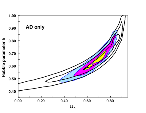
Figure 1: Joint likelihood contours (Bayesian), with CMB only (solid lines, showing $1\sigma$, $2\sigma$, $3\sigma$ contours) and CMB+LSS (filled) for purely adiabatic initial conditions.

From the Bayesian analysis, one concludes that CMB and LSS together require a non-zero cosmological constant at very high significance, more than $7\sigma$ for the points in our grid! Note that the ML point has a reduced chi-square $\hat{\chi}^{2}_{F=56}=0.59$, significantly less than $1$.

The frequentist analysis, however, excludes a much smaller region of parameter space (Fig. 2). The frequentist contours must be drawn for the effective number of dof, i.e., using the number of effectively independent data points. We can therefore roughly take into account a $10\%$ correlation, which is the maximum correlation between data points given in Arch ; Net , by replacing $F$ by the effective number of dof, $F_{\rm eff}=0.9N-M$, and rounding to the next larger integer (to be conservative). One could argue that the BOOMERanG and Archeops data points are not completely independent, since BOOMERanG observed a portion of the same sky patch as measured by Archeops. This possible correlation is difficult to quantify, but should not be too important since the sky portion observed by Archeops is a factor of 10 larger than BOOMERanG’s and therefore we ignore it here. Fig. 2 is drawn with $F_{\rm eff}=31$ for CMB alone and $F_{\rm eff}=50$ for CMB+LSS, but we have checked that our results do not change much if we use a $5\%$ correlation. It is interesting to note that there are regions in Fig. 2 which are excluded with a certain confidence by CMB data alone but are no longer excluded at the same confidence when we include LSS data. In other words, it would seem that taking into account more data and therefore more knowledge about the universe, does not systematically exclude more models, i.e., the CMB+LSS contours are not always contained in the CMB alone contours. This apparent contradiction vanishes when one realizes that the confidence limits on, e.g., $\Omega_{\Lambda}$ alone in the frequentist approach are just the projection of the confidence contours of Fig. 2 on the $\Omega_{\Lambda}$ axis. One can readily verify in Fig. 2 that the confidence limits for the combined data-set are always smaller than the ones for CMB data alone. There are points with $\Omega_{\Lambda}=0$ and $h\simeq 0.40$ which are still compatible within $2\sigma$ with both LSS and CMB data, at the price of pushing somewhat the other parameters. In the best fit with $\Omega_{\Lambda}=0$ shown in Fig. 3, one has to live with a red spectral index $n_{\rm S}=0.80$. Furthermore, the calibration of the BOOMERanG and Archeops data points is reduced in this fit by $34\%$ and $26\%$, respectively, i.e., more than 3 times the quoted $1\sigma$ systematic error.

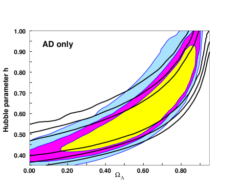
Figure 2: Confidence contours (frequentist) with CMB only (solid lines, $1\sigma$, $2\sigma$, $3\sigma$ contours and $F_{\rm eff}=31$) and CMB+LSS (filled, $F_{\rm eff}=50$) for purely adiabatic initial conditions.

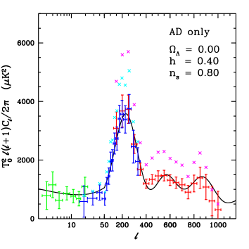
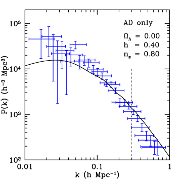
Figure 3: Best fit with $\Omega_{\Lambda}=0$ and purely AD initial conditions, compatible with CMB and LSS data within $2\sigma$ confidence level. In the lower panel, only the 2dF data points left of the vertical, dotted line — i.e., in the linear region — have been included in the analysis. Note the low first acoustic peak due to the joint effect of the red spectral index and of the absence of early ISW effect. In this fit, the calibration of BOOMERanG (red errorbars) and Archeops (blue errorbars) has been reduced by $34\%$ and $26\%$, respectively. This is more than 3 times the quoted $1\sigma$ calibration errors for both experiments. To appreciate the difference, we plot the non recalibrated value of the BOOMERanG and Archeops data points as light blue and magenta crosses, respectively. In the upper panel, green errorbars are the COBE measurements. Even though the fit is “by eye” very good, it seems highly unlikely that the calibration error is so large.

In both cases, it is clear that one can exploit the $\Omega_{\Lambda}$, $h$ degeneracy to fit CMB data alone with a model having $\Omega_{\Lambda}=0$. For a flat universe like the one we are considering, one has then to go to a much smaller value of the Hubble parameter than the one indicated by other measurements, most notably the HST Key Project HST , which gives $h=0.72\pm 0.08$. The LSS data are mainly sensitive to the shape parameter $\Gamma\sim 0.2$. Hence LSS with $\Omega_{\rm m}=1.0$ would require an even lower value of $h$ which is not compatible with CMB. Therefore inclusion of LSS data tends to exclude any flat model without a cosmological constant. Summing up, for purely adiabatic initial conditions the Bayesian approach gives very strong support to $\Omega_{\Lambda}\neq 0$; in the more conservative frequentist point of view, while $\Omega_{\Lambda}\neq 0$ cannot be excluded with very high confidence, present LSS and CMB data start to be incompatible with a flat universe with vanishing cosmological constant. These conclusions are in qualitative agreement with previous works netti ; pryke ; max ; novos ; RM ; MCMC ; Arch2 .

In the next section we investigate the stability of those well known results with respect to inclusion of non-adiabatic initial conditions.

III.2 Isocurvature modes

We now enlarge the space of models by including all possible isocurvature modes with arbitrary correlations among themselves and the adiabatic mode as described in the previous section. We first consider CMB data only and maximize over initial conditions. The number of parameters increases by nine and the number of dof decreases correspondingly with respect to the purely AD case considered above. Likelihood (Bayesian, see Fig. 4) and confidence (frequentist, see Fig. 7) contours widen up somewhat along the degeneracy line. The enlargement is less dramatic than for other parameter choices, see, e.g., Ref. TRD1 where the degeneracy in $\omega_{\rm b},h$ was analyzed. This is partially due to our prior of flatness which reduces the space of models to the ones which are almost degenerate in the angular diameter distance. Most of our models have the first acoustic peak of the adiabatic mode already in the region preferred by experiments. Hence in most of the fits isocurvature modes play a modest role, especially in the parameter regions with large $\Omega_{\Lambda}$, $h$ (cf Fig. 9 and the discussion below). Nevertheless, because of the $\Omega_{\Lambda}$, $h$ degeneracy, even a modest widening of the contours along the degeneracy line results in an important worsening of the likelihood limits. The ML point does not depart very much from the purely adiabatic case, but now we cannot constrain $\Omega_{\Lambda}$ at more than $1\sigma$ (Bayesian, CMB only):

$$\Omega_{\Lambda}=0.85_{-0.35}^{+0.05}\mbox{ at $1\sigma$, }$$ (12)

and no limits for $0.0\leq\Omega_{\Lambda}\leq 0.95$ at higher confidence.

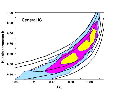
Figure 4: Joint likelihood contours (Bayesian) with general isocurvature initial conditions, with CMB only (solid lines, $1\sigma$, $2\sigma$, $3\sigma$) and CMB+LSS (filled). The disconnected $1\sigma$ region is an artificial feature due to the grid resolution.

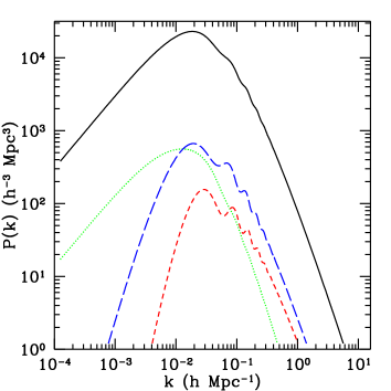
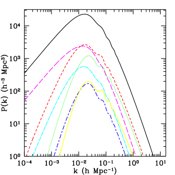
Figure 5: Dark matter power spectra of the different auto- (upper panel) and cross-correlators (lower panel) for a concordance model with $\Omega_{\Lambda}=0.70$, $h=0.65$, $n_{\rm S}=1.0$, $\omega_{\rm b}=0.020$, with the corresponding CMB power spectrum COBE-normalized (see the text for details). The color codes are as follows: in the upper panel, AD: solid/black line, CI: dotted/green line, NID: short-dashed/red line, NIV: long-dashed/blue line; in the lower panel, AD: solid/black line (for comparison), $<{\rm AD},{\rm CI}>$: long-dashed/magenta line, $<{\rm AD},{\rm NID}>$: dotted/green line, $<{\rm AD},{\rm NIV}>$: short-dashed/red line, $<{\rm CI},{\rm NID}>$: dot-short dashed/blue line, $<{\rm CI},{\rm NIV}>$: dot-long dashed/light-blue line, and $<{\rm NID},{\rm NIV}>$: solid/yellow line. The adiabatic mode is by far dominant over all others.

In Fig. 5 we plot the dark matter power spectra of the different auto- (upper panel) and cross-correlators (lower panel) for a concordance model. The norm of each pure mode (AD, CI, NID, NIV) is chosen such that the corresponding CMB power spectrum is COBE-normalized. The cross-correlators are normalized according to totally correlated spectra, i.e.

$$A_{(\rm{X},\rm{Y})}=\sqrt{A_{\rm{X}}A_{\rm{Y}}/2}~{},$$ (13)

where $A_{(\rm{X},\rm{Y})}$ denotes the norm of the cross-correlator between the modes $X$,$Y$ and $A_{\rm X}$ the norm of the pure mode $X$. The CMB power spectrum for this set of cosmological parameters can be found in Ref. BMT2 . A crucial result is that the COBE-normalized amplitude of the AD matter power spectrum is nearly two orders of magnitude larger than the isocurvature contribution. The main reason for this is the amplitude of the Sachs Wolfe plateau which is about $\frac{1}{3}\Psi$ for adiabatic perturbations and $2\Psi$ for isocurvature perturbations. Here $\Psi$ is the gravitational potential. This difference of a factor of about $36$ in the power spectrum on large scales is clearly visible in the comparison of $P_{\rm AD}$ and $P_{\rm CI}$ (the difference increases at smaller scales). The case of the neutrino modes is even worse since they start up with vanishing dark matter perturbations. That the CDM isocurvature matter power spectrum is much lower than the adiabatic one has been known for some time (see e.g. Ref. banday ). However, it was not recognized before that the same holds true for the neutrino isocurvature matter power spectra as well, and – more importantly – that this leads to a way to break the strong degeneracy among initial conditions which is present in the CMB power spectrum alone.

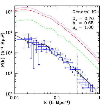
Figure 6: Concordance model fit with general IC and LSS data only. The total spectrum (solid/black) is the result of a large cancellation of the purely AD part (long-dashed/red) by the large, negative sum of the various correlators (dotted/magenta, plotted in absolute value). The short-dashed/green curve is the sum of the three pure isocurvature modes, CI, NID and NIV. Note that the resulting total spectrum is less than one tenth of the purely adiabatic part.

In an analysis with general initial conditions including LSS data only we obtain very broad likelihood and confidence contours which exclude only the lower right corner of the $(\Omega_{\Lambda},h)$ plane. In contrast to the CMB power spectrum, the matter power spectrum can be fitted with extremely high adiabatic and isocurvature contributions, which are then typically cancelled by large anti-correlations between the spectra. This behavior is exemplified for a model with general IC and $\Omega_{\Lambda}=0.70$, $h=0.65$, $n_{\rm S}=1.0$ in Fig. 6. The best fits with LSS data only are dominated by large isocurvature cross-correlations. Clearly, the resulting CMB power spectrum is highly inconsistent with the COBE data. Hence such “bizarre” possibilities are immediately ruled out once we include CMB data. Conversely, moderate isocurvature contributions can help fitting the CMB data, and do not influence the matter power spectrum, which is completely dominated by the AD mode alone. Combining CMB and LSS data (see Fig. 4) we find now (Bayesian, mixed IC):

$$\Omega_{\Lambda}=0.65_{-0.25}^{+0.22}\mbox{ at $2\sigma$ $\quad$ and $\quad$}_{-0.48}^{+0.25}\mbox{ at 3$\sigma$}.$$ (14)

The likelihood limits are larger than for the purely adiabatic case but it is interesting that the Bayesian analysis still excludes $\Omega_{\Lambda}=0$ at more than $3\sigma$ even with general initial conditions, for the class of models considered here. Because of the above explained reason, the widening of the limits is not as drastic as one might fear. Therefore, combination of CMB and LSS measurements turn out to be an ideal tool to constrain the isocurvature contribution to the initial conditions.

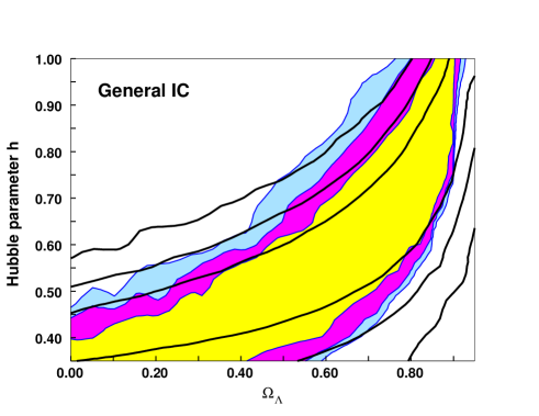
Figure 7: Confidence contours (frequentist) with general isocurvature initial conditions with CMB only (solid lines, $1\sigma$, $2\sigma$, $3\sigma$ contours $F_{\rm eff}=22$) and CMB+LSS (filled, $F_{\rm eff}=41$).

From the frequentist point of view, one notices that the region in the $\Omega_{\Lambda},h$ plane which is incompatible with data at more than $3\sigma$ is nearly independent on the choice of initial conditions (compare Fig. 2 and Fig. 7). Enlarging the space of initial conditions seemingly does not have a relevant benefit on fitting present-day data with or without a cosmological constant. The reason for this is that the (COBE-normalized) matter power spectrum is dominated by its adiabatic component and therefore the requirement $\Omega_{\rm m}h\sim 0.2$ remains valid. In Fig. 8 we plot the best fit model with general initial conditions and $\Omega_{\Lambda}=0$. We summarize our likelihood and confidence intervals on $\Omega_{\Lambda}$ (this parameter only) in Table 1.

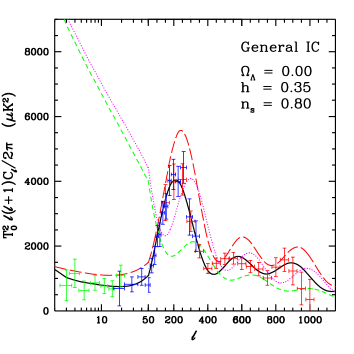
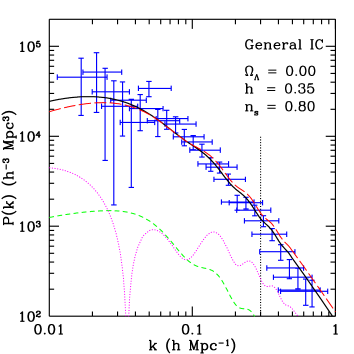
Figure 8: Best fit with general IC and $\Omega_{\Lambda}=0$. As for purely AD, even with general IC the absence of the cosmological constant suppresses in an important way the height of the first peak. In both panels we plot the best total spectrum (solid/black), the purely AD contribution (long-dashed/red), the sum of the pure isocurvature modes (short-dashed/green) and the sum of the correlators (dotted/magenta, multiplied by $-1$ in the upper panel and in absolute value in the lower panel). The matter power spectrum is completely dominated by the AD mode, while the correlators play an important role in cancelling unwanted contributions in the CMB power spectrum at the level of the first peak and especially in the COBE region. For this model we have $\beta=0.39$, while the BOOMERanG and Archeops calibrations are reduced by $28\%$ and $12\%$, respectively.

In Fig. 9 we plot the isocurvature contribution to the best fit models with CMB and LSS in terms of the parameter $\beta$ defined in Eq. (6). The best fit with $\Omega_{\Lambda}=0$ has an isocurvature contribution of about $40\%$.

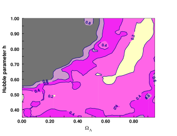
Figure 9: Isocurvature content $0.0\leq\beta\leq 1.0$ of best fit models with CMB and LSS data. The contours are for $\beta=0.20,0.40,0.60,0.80$ from the center to the outside.

It would be of great interest to investigate whether the result $\Omega_{\Lambda}\neq 0$ is robust with respect to addition of general initial conditions in an open universe TRDprep .

Table 1: Results for the likelihood (Bayesian) and confidence (frequentist) intervals for $\Omega_{\Lambda}$ alone (all other parameters maximized). A bar, $-$, indicates that at the given likelihood/confidence level the analysis cannot constraint $\Omega_{\Lambda}$ in the range $0.0\leq\Omega_{\Lambda}\leq 0.95$. Where the quoted interval is smaller than our grid resolution, an interpolation between models has been used.

AD only
		Bayesian			Frequentist
Data-set	$\quad\Omega_{\Lambda}$	$1\sigma$	$2\sigma$	$3\sigma$	$1\sigma$	$2\sigma$	$3\sigma$	$F$	$\chi^{2}/F$
CMB+flatness	$0.80$	${}_{-0.08}^{+0.08}$	${}_{-0.35}^{+0.10}$	${}_{\quad-}^{+0.12}$	$<0.93$	$-$	$-$	$35$	$0.58$
CMB +LSS+flatness	$0.70$	${}_{-0.05}^{+0.05}$	${}_{-0.17}^{+0.13}$	${}_{-0.27}^{+0.15}$	$0.15<\Omega_{\Lambda}<0.90$	$\quad<0.92$	$\quad<0.92$	$56$	$0.59$
General IC
CMB+flatness	$0.85$	${}_{-0.35}^{+0.05}$	$-$	$-$	$-$	$-$	$-$	$26$	$0.74$
CMB +LSS+flatness	$0.65$	${}_{-0.10}^{+0.15}$	${}_{-0.25}^{+0.22}$	${}_{-0.48}^{+0.25}$	$<0.90$	$<0.92$	$\quad<0.95$	$47$	$0.67$

IV Conclusions

The conclusions of this work are threefold. The first one is not new, but seems to be dangerously forgotten in recent cosmological parameters estimation literature: namely that likelihood contours cannot be used as “exclusion plots”. The latter are usually substantially wider, less stringent. A more rigorous possibility are frequentist probabilities, which however suffer from the dependence on the number of really independent measurements which is often very difficult to come by.

Secondly, we have found that in COBE-normalized fluctuations, the matter power spectrum has negligible isocurvature contributions and is essentially given by the adiabatic mode. Hence the shape of the observed matter power spectrum still requires $\Omega_{\rm m}h\simeq 0.2$, independent of the choice of initial conditions. Due to this behavior, the condition $\Omega=\Omega_{\Lambda}+\Omega_{\rm m}=1$ requires either a cosmological constant or a very small value for the Hubble parameter, independently from the isocurvature contribution to the initial conditions.

The third conclusion from our work are the following results for the presence of a cosmological constant: For flat models, a likelihood (Bayesian) analysis strongly favors a non-vanishing cosmological constant. Even if we allow for isocurvature contributions with arbitrary correlations, a vanishing cosmological constant is still excluded at more than $3\sigma$. If we would allow for open models, a significant contribution from the NIV mode which has the first acoustic peak at $\ell=170$ in flat models, possibly could at the same time give a good fit to CMB data and allow for the observed shape parameter $\Gamma$ with a reasonable value of $h$. For technical reasons we shall study this case in a forthcoming paper TRDprep .

The situation changes considerably in the frequentist approach. There, even for purely adiabatic models, $\Omega_{\Lambda}=0$ is still within $3\sigma$ for a value of $h\leq 0.48$ which is marginally defendable. The conclusion does not change very much when we allow for generic initial conditions.

- (1) A. Einstein, Sitzungsber. Preuss. Akad. Wiss. 142, (1917).
- (2) A.G. Riess et al., Astron. J. 116, 1009 (1998).
- (3) S. Perlmutter et al., Astrophys. J. 517, 565 (1999).
- (4) B. Ratra and P.J.E. Peebles, Phys. Rev. D37, 3406 (1988); C. Wetterich Nucl. Phys. B302, 668 (1988).
- (5) P.G. Ferreira and M. Joyce, Phys. Rev. Lett. 79, 4740 (1997).
- (6) R.R. Caldwell, R. Dave and P. Steinhardt, Phys. Rev. Lett. 80, 1582 (1998).
- (7) C.B. Netterfield et al., Astrophys. J. 571, 604 (2002).
- (8) J.A. Rubino-Martin et al., preprint astro-ph/0205367.
- (9) A. Meszaros, Astrophys. J. (accepted), preprint astroph/0207558.
- (10) J. Barriga, E. Gaztanaga, M. Santos and S. Sakar, Mon.Not.Roy.Astron.Soc. 324 977 (2001).
- (11) M. Bucher, K. Moodley, and N. Turok, Phys. Rev. D62, 083508 (2000).
- (12) M. Bucher, K. Moodley, and N. Turok, Phys. Rev. Lett. 87 191301 (2001).
- (13) R. Trotta, A. Riazuelo, and R. Durrer Phys. Rev. Lett. 87 231301 (2001).
- (14) A.T. Lee et al., preprint astro-ph/0104459.
- (15) N.W. Halverson et al., preprint astro-ph/0104489 (2001).
- (16) P.F. Scott et al., preprint astro-ph/0205380; A. Taylor et al., preprint astro-ph/0205381.
- (17) T.J. Pearson et al., peprint astro-ph/0205388.
- (18) A. Benoît et al., preprint astro-ph/0210305.
- (19) G.F. Smoot et al., Astrophys. J. 396, L1 (1992); C.L. Bennett et al., Astrophys. J. 430, 423 (1994); M. Tegmark and A.J.S. Hamilton, in 18th Texas Symposium on relativistic astrophysics and cosmology, edited by A.V. Olinto et al., pp 270 (World Scientific, Singapore, 1997).
- (20) M. Tegmark, A. Hamilton and Y. Xu, Month. Not. R. Astron. Soc. (accepted), preprint astro-ph/0111575.
- (21) S. Burles, K.M. Nollet, and M.S. Turner, Astrophys. J. 552, L1 (2001).
- (22) C. Gordon, and A. Lewis, preprint astro-ph/0212248.
- (23) G.J. Feldman and R.D. Cousins, Phys. Rev. D57, 3873-3889 (1998).
- (24) A.G. Frodesen, O. Skjeggestad and H. Tofte, Probability and Statistics in Particle Physics (Universitetsforlaget, Bergen-Oslo-Tromso 1979).
- (25) M.G. Kendall, and A. Stuart, The advanced theory of statistics, Vol. 2, 4th ed. (High Wycombe, London, 1977).
- (26) A. Lewis, and S. Bridle, Phys. Rev. D66, 103511 (2002).
- (27) A. Melchiorri, and L.M. Griffiths, New Astronomy Reviews 45, 4-5 (2001).
- (28) W. Freedman et al., Astrophys. J. 553, 47 (2001).
- (29) C.B. Netterfield et al., Astrophys. J. 571, 604 (2002).
- (30) C. Pryke et al., Astrophys. J. 568, 46 (2002).
- (31) X. Wang, M. Tegmark, and M. Zalderriaga, Phys. Rev. D65, 123001 (2002).
- (32) R. Durrer, B. Novosyadlyj, and S. Apunevich, Astrophys. J. 583, 1 (2003).
- (33) J.A. Rubino-Martin et al., preprint astro-ph/0205367.
- (34) A. Lewis and S. Bridle, preprint astro-ph/0205436.
- (35) A. Benoît et al., preprint astro-ph/0210306.
- (36) R. Stompor, J.A. Banday, K.M. Gorsky, Astrophys. J. 463, 8 (1996).
- (37) R. Trotta, A. Riazuelo, and R. Durrer, in preparation.
- (38) Archeops homepage: http://www.archeops.org/ .
- (39) M. Tegmark site: http://www.hep.upenn.edu/~max/ .