GRS 1915+105: The brightest Galactic black hole

Abstract

We compare the evolution of spectral shape with luminosity in GRS 1915+105 with that of ‘normal’ black holes. The pathological variability of GRS 1915+105, which probably indicates a disc instability, does not require that GRS 1915+105 belongs in a different class to all the other objects. At comparable fractions of Eddington luminosity its spectra and (more importantly) apparent disc stability, are both similar to that seen in the ‘normal’ black holes. Its unique limit-cycle variability only appears when it radiates at uniquely high (super-Eddington) luminosities.

1 Introduction

GRS 1915+105 is a spectacularly variable accreting black hole in our Galaxy. It was first detected in X-rays by the WATCH all sky monitor on board the GRANAT satellite in 1992 (Castro-Tirado, Brandt & Lund 1992), but achieved fame when radio observations showed it to be the first galactic superluminal source, implying relativistic plasma ejection (Mirabel & Rodríguez 1994). Several more superluminal jet sources have since been found (GRO J1655–40, XTE J1748–288, V4641 Sgr), while a much larger number of black holes (the microquasars) show jet-like radio morphology (e.g. Mirabel & Rodríguez 1999). Mildly relativistic jets are now recognized as a common feature of black holes at high mass accretion rates (Fender & Kuulkers 2001).

However, GRS 1915+105 is still unique in its variability properties. On long timescales, its outburst duration of over 10 years is unprecedented, and completely at odds with the predictions of the disc instability models which can successfully describe some aspects of the other black hole transient outbursts (King & Ritter 1998; Dubus, Hameury & Lasota 2001; Esin, Lasota & Hynes 2000). On short timescales, the X-ray variability is even more singular, showing episodes where it continually switches between states in a quasi–regular way (Greiner, Morgan & Remillard 1996; Chen, Swank & Taam 1997). Belloni et al. (1997a) showed that these rapid changes were associated with the accretion disc spectrum switching from hot and bright, implying a small inner disc radius, to cooler and dimmer, with a larger inferred radius. They interpreted this as the result of a limit-cycle instability in the inner accretion disc, such that it is continually emptying and refilling.

Following Belloni et al. (1997a, b), most models for the origin of this unique limit-cycle behaviour of the accretion disc have concentrated on the radiation pressure instability in a standard Shakura-Sunyaev accretion disc (Shakura & Sunyaev 1973). In the $\alpha$ disc prescription the viscous heating is proportional to the total pressure $P_{\rm tot}=P_{\rm gas}+P_{\rm rad}$, i.e. the sum of the gas and radiation pressures. Where radiation pressure dominates the heating rate is dramatically sensitive to temperature ($P_{\rm rad}\propto T^{4}$ compared to $P_{\rm gas}\propto T$), and the radiative and convective cooling in the disc cannot keep pace. By itself, this would just lead to the classic thermal-viscous instability (Lightman & Eardley 1974; Shakura & Sunyaev 1976). However, there is another stable disc solution at high temperatures, where optically thick advective cooling becomes important (Abramowicz et al. 1988). Putting all this together at a given radius and $\alpha$ gives rise to an S-curve on a plot of disc surface density, $\Sigma$ versus mass accretion rate through the disc, $\dot{m}\propto T^{4}$. The lower, middle and upper branches of the S corresponding to heating $\propto P_{\rm gas}$ balanced by radiative cooling (stable), heating $\propto P_{\rm rad}$ balanced by radiative cooling (unstable) and heating $\propto P_{\rm rad}$ balanced by advective cooling (stable; Abramowicz et al. 1988; Chen et al. 1995). No steady state equilibrium solution is possible at mass accretion rates corresponding to the middle branch. Instead there is a continual limit-cycle with the material switching between the two stable states, one which has too high a mass accretion rate, leading to the emptying of the disc, and one with too low as mass accretion rate, so the disc refills.

However, it is difficult to understand why the radiation pressure instability is not apparent in other black hole X-ray transients (see e.g. Gierliński & Done 2003b, hereafter GD03). The only features distinguishing black holes are mass and spin. GRS 1915+105 is the most massive galactic black hole known at $\sim$14 M_⊙ (Greiner, Cuby & McCaughrean 2001a), but this is not significantly larger than the typical $10M_{\odot}$ of the other black holes (Bailyn et al. 1998). It may well be spinning close to maximal, but so may GRO J1655–40 (Zhang, Cui & Chen 1997; Cui, Zhang & Chen 1998). If the difference is not in the black hole itself, then it must be connected to the accretion flow. GRS 1915+105  accretes at high fractions of the Eddington limit, but so do many other black hole transients (see e.g the review by Tanaka & Lewin 1995). GRS 1915+105 has a jet, which is clearly linked to limit-cycle behaviour of the disc (Pooley & Fender 1997; Eikenberry et al. 1998), but the ratio of radio to X-ray power is similar to that of other X-ray transients (Fender & Kuulkers 2001). Why then is the variability from GRS 1915+105 unique?

Recently, Done & Gierliński (2003; hereafter DG03) used the huge Rossi X-ray Timing Explorer (RXTE) database to systematically analyze the spectra of many black hole systems. These were all consistent with the same spectral evolution as a function of Eddington luminosity fraction, $L/L_{\rm Edd}$, so these form a ‘normal’ black hole sample for comparison with GRS 1915+105. Here we analyze the RXTE data on GRS 1915+105 and plot it together with the ‘normal’ black holes. We show that GRS 1915+105 is unique in being the only black hole binary which spends any considerable time above $L/L_{\rm Edd}\sim 1$, and speculate that this is the trigger for the limit-cycle variability in GRS 1915+105.

The reason GRS 1915+105 alone gets to such consistently high mass accretion rates can be simply related to its evolutionary state. The secondary is a giant (Greiner et al. 2001b), so Roche lobe overflow occurs in a much wider binary than for a main sequence star. The 33.5-day period of GRS 1915+105 is by far the longest of any low-mass X-ray binary (LMXB) known. This implies a huge disc size, as the outer radius is set by tidal truncation. During quiescence the disc builds up an immense reservoir of mass, which can fall onto the black hole when the outburst is triggered (King & Ritter 1998). The underlying cause of all the unique long and short-term variability of GRS 1915+105 is then ultimately linked to the evolution of the huge disc structure, which can contain enough material to maintain super-Eddington accretion rates over timescales of tens of years.

2 Data selection and reduction

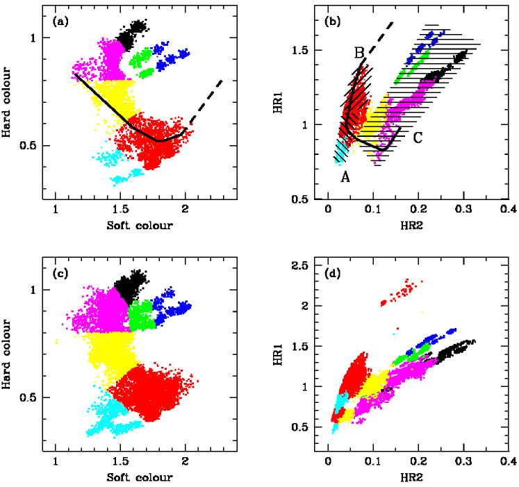
Figure 1: (a) shows the intrinsic colour-colour diagram for each 128-s spectrum of GRS 1915+105  using the data selection of B00. These colours are corrected for interstellar absorption and for the instrument response, giving a measure of the intrinsic spectral slope in the 3–6.7 keV (soft colour) and 6.7–16.0 keV (hard colour) bandpass (see DG03). (b) shows the corresponding instrument colour-colour diagram as used by B00. Regions marked in the same colours in panels (a) and (b) correspond to the same data. The shading indicates the spectral states A, B and C defined by B00, while the solid/dotted line is again from B00, indicating the path of a typical instability. The B00 data are on 1-s resolution, and so their colours can follow the very rapid variability in the flares (indicated by the dotted line) which are not sampled by the 128-s spectra used here. Panels (c) and (d) reproduce panels (a) and (b) but for all observations from PCA epochs 2–4. The intrinsic diagram looks very similar, but the instrument diagram is very different due to gain changes in the detector. There is no longer a unique correspondence between the intrinsic spectral shape and instrument count ratios (e.g. the red region indicating a particular spectral shape is split into three separate regions in instrument counts).

RXTE has been in operation since January 1996. The Proportional Counter Array (PCA) on board RXTE had undergone several major gain changes, marking five instrument epochs. Here we analyze all PCA data before the end of PCA epoch 4, i.e. observations between 1996 April 6 and 2000 May 11 (epoch 5 is marked by the loss of the propane layer for detector 0). We use ftools 5.2 and follow standard data reduction procedure as recommended by the RXTE team. To maximize the number of observations which can be used we select data from PCA detector 0 only, as it is switched on most of the time. The source is dramatically variable so we extract data in 128-s bins, giving a quite overwhelming number of 16489 individual spectra. There is variability on shorter timescales (see e.g. Belloni et al. 2000; hereafter B00) but this is the shortest timescale on which the spectra are generally limited by systematic errors (set to 1 per cent) rather than statistical errors below 10 keV. We also accumulate both light curves and spectra for each of the 500 separate pointings, designated by unique observation IDs, typically each giving a few kiloseconds of data. The light curves for each observation ID are extracted over 3–20 keV with the 16-second time resolution of the Standard 2 data.

3 Spectral modelling

We use xspec (Arnaud 1996) to fit the PCA data in 3–20 keV range with 1 per cent error added in each energy channel to represent the systematic uncertainties of the detector response. We assume the abundances of Anders & Ebihara (1982) unless stated otherwise, and fix the interstellar galactic absorbing column at $4.7\times 10^{22}$ cm^-2 (Chaty et al. 1996). For calculating luminosities we assume distance of 12.5 kpc (Mirabel & Rodríguez 1994 but see Fender et al. 1999). All parameter ranges are quoted for $\Delta\chi^{2}$ = 2.7.

Following DG03 we fit a physically motivated continuum model consisting of a multicolour disc spectrum which also forms the seed photons for Compton scattering to higher energies. We use the diskbb model (Mistuda et al. 1984) to describe the disc emission. The temperature is constrained to $kT_{\rm disc}\geq 0.4$ keV. so as not to produce an unphysically large component outside of the energy range of the PCA data. For Comptonization we use thcomp (not included in the standard distribution of xspec, see Zdziarski, Johnson & Magdziarz 1996), parameterized by asymptotic photon spectral index ($\Gamma\geq 1$) and electron temperature ($kT_{\rm comp}\leq$ 100 keV).

3.1 Simple model

The physically motivated continuum model does not fully describe the observed spectra from X-ray binaries as there is also Compton reflection from the disc. Following DG03 we approximate this by adding a broad Gaussian line (width fixed at $0.5$ keV) and smeared edge (index for photoelectric cross-section fixed at -2.67 and smearing width of 7 keV; see Ebisawa 1991). This model spectrum is described as M1 in Table 2 and throughout the text.

We use this to fit each 128-s spectrum from GRS 1915+105. It gives a good description of most of the data; only 5 per cent have reduced $\chi^{2}/\nu>1.5$ (where $\nu$ is number of degrees of freedom). We follow the approach of DG03 in compressing all the resulting spectral information from the model fits into two intrinsic colours, which are calculated by integrating the (absorption corrected) model flux over 4 energy bands (3–4, 4–6.4, 6.4–9.7, 9.7–16 keV) to form soft and hard colours. These roughly describe the unabsorbed spectral slope from 3–6.4 keV and 6.4–16 keV, respectively.

This method contrasts with that of the more usual instrument colours, which are defined using the ratios of observed counts in given energy bands (as opposed to modelled flux ratios). Both methods have their advantages and disadvantages. The advantage of our method is that modelling corrects for both instrument response and absorption in a single step, and gives colours which reflect the underlying source spectrum. Thus many objects, with data taken from many different instruments and/or gain epochs, with very different absorption columns, can be easily plotted together on the same diagram. Instrument colours can be modified to correct for different gain epochs (e.g. Di Salvo et al. 2003, van Straaten et al. 2003), but different absorptions prevent a straightforward comparison of many different objects. Another advantage of our approach is that the model spectra allow us to estimate the bolometric luminosity, which is surely a major physical driver of the spectral evolution. The disadvantage of course is that these luminosities are model dependent (though the colours are not as long as absorption does not substantially affect the spectrum above 3 keV: DG03). More importantly, the requirement for good signal-to-noise spectra for the model fitting means that the intrinsic colours have lower time resolution than the instrument ones.

Belloni et al. (2000: hereafter B00) used instrument colours for their major study of the variability of GRS 1915+105 as seen in Epoch 3. Fig. 1a and b shows a comparison of our derived intrinsic colours (defined by model flux ratios) for the Epoch 3 data with those of the instrument colours (defined by observed count ratios) as used by B00. Data from different regions of Fig. 1a are colour-coded, so that their corresponding position on Fig.1b can easily be identified, so that we can use the B00 insights into the nature of the variability as a function of colour. In particular, they unified the incredibly rich variability patterns into transitions between 3 main spectral states – A, B and C which they associate with a disc instability (Belloni et al. 1997a, b). These states are shown by the shaded areas in Fig. 1b, while the thick black line shows the track in colour-colour space of a dramatic transition ($\lambda$-type variability, taken from observation ID 10408-01-38-00 as shown in figure 2m of B00). The dotted line shows the continuation of this track which is seen in high time resolution data. B00 are able to get a good instrument colour on 1-s time resolution, as opposed to the 128-s spectra needed for the model fitting used here.

While we cannot follow the most rapid variability, Figs. 1c and 1d show some of the power of our intrinsic colour approach when combining all the data from Epochs 2–4. The intrinsic colour-colour diagram is very similar to that derived just from B00 data (compare panels a and c in Fig. 1), whereas the straightforward instrument colours are strongly affected, with data from different Epochs ending up at very different position in the diagram (Epoch 2 has much higher HR1 and HR2 than epoch 3, while Epoch 4 has much lower HR1 and HR2). While these gain change effects can be corrected for (di Salvo et al. 2003; van Straaten et al. 2003), the key issue in this paper is that the unabsorbed flux ratios shown in Fig. 1c can be directly compared with the unabsorbed colours from many other black holes given in e.g. DG03. We can use this straightforward comparison of multiple objects to search for the differences between GRS 1915+105 and the ‘normal’ black holes which underlay its unique variability.

3.2 Variability as a function of colour

B00 show that the unique limit-cycle variability of GRS 1915+105 occurs in only $\sim$50 per cent of the data. Rather than do a detailed classification of the variability pattern (as in B00), we simply parameterize the variability in a given observation (one individual RXTE pointing with unique observation ID) by calculating the fractional r.m.s. (variance divided by mean intensity) from its light curve with resolution of 16 s. Some of the observations are too short for this to be reliable, so we restrict this to light curves in which there are more than 128 data points (i.e. over 2048 s of data). This fractional r.m.s. represents the integral of the power spectrum from frequencies lower than 1/2048 to 1/32 Hz. The low frequency power spectrum is generally flatter than $f^{-1}$ (e.g. Morgan et al. 1997) so the fractional r.m.s. is not strongly dependent on the length of the light curve.

Assuming that the power spectrum is stable for each type of variability, we can use the individual observation IDs identified by B00 as being characteristic of each class to get an estimate of their fractional r.m.s.. The state transition classes $\mu,\theta,\lambda,\kappa,\rho,\nu,\alpha,\beta,\delta$ and $\gamma$ have $17,36,52,54,35,47,27,49,16$ and $7$ per cent variability, respectively, while the single state classes $\phi$ and $\chi$ have $7$ and $3$ per cent, respectively. While it is plain that our crude fractional r.m.s. criteria cannot make subtle distinctions between the types of state transition, nevertheless it is clear that restricting the fractional r.m.s. to less than 5 per cent will select typically only the $\chi$ stable state (through may include a little contamination by the $\phi$ and $\gamma$ type of variability), while selecting fractional r.m.s. greater than 40 per cent will pick out the dramatic state transition variability of type $\lambda,\kappa,\nu,\beta$ (perhaps with a little contribution from $\theta$ and $\rho$ states. It is these dramatic variability patterns which are unique to GRS 1915+105 which we want to identify.

The intrinsic colours for the resulting 292 spectra were found using the model described above. Obviously, some of the spectra are averaged over periods of high variability, including the limit-cycle spectral transitions. These do not represent real physical spectra: the average of two blackbodies of different temperatures is not a blackbody at the average temperature, nor is the average of two power laws of different spectral slopes given by a single power law of the average slope! Instead, the colours extracted from these spectra give the time averaged position of the source on the colour-colour diagram. Fig. 2 shows these intrinsic colours, with r.m.s. variability indicated. This illustrates the result of B00 that the limit-cycle variability which is unique to GRS 1915+105 is associated with very particular spectral shapes which mark out the track of the instability.

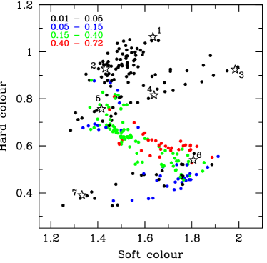
Figure 2: The intrinsic colour-colour diagram of the individual PCA pointings with $>2048$ s of data. These cover the full range of spectral behaviour seen in Fig. 1c. The points are colour coded according to the amount of fractional r.m.s. variability present in the 3–20 keV light curve for each observation as given in the key in the top-left corner of the figure. The numbered stars show the positions of the individual spectra used for spectral analysis in Sec. 3.3.

3.3 Detailed analysis of selected spectra

Obs.	Obs. ID	Live time	Count rate	r. m. s.
		(s)	(s-1)	per cent
1	30703-01-34-00	2400	873$\pm$2	4.0$\pm$0.3
2	20402-01-29-00	4208	1157$\pm$3	2.9$\pm$0.2
3	10408-01-27-00	7552	1562$\pm$3	1.9$\pm$0.1
4	30402-01-09-00	3712	1751$\pm$4	1.5$\pm$0.1
5	30184-01-01-00	15184	1896$\pm$4	1.3$\pm$0.1
6	20402-01-55-00	7552	3267$\pm$8	3.9$\pm$0.2
7	30703-01-08-00	4000	1099$\pm$3	3.5$\pm$0.2

Table 1: Log of seven PCA observations selected for detailed spectral analysis. The root mean square variability is calculated from 3–20 keV light curves with 16-s resolution.

Model	xspec components	Description
M1	wabs*smedge*(diskbb+thcomp+gaussian)	Simple model of multicolour disc with thermal Comptonization. Reflection features are approximated by broad Gaussian and smeared edge. Absorption with solar abundances fixed at $N_{H}=4.7\times 10^{22}$ cm-2.
M2	wabs*(diskbb+thcomp+relrep)	Multicolour disc, thermal Comptonization and its ionized Compton reflection, relativistically smeared. Absorption with solar abundances fixed at $N_{H}=4.7\times 10^{22}$ cm-2.
M3	varabs*(diskbb+thcomp+relrep)	The same as M2, but with anomalous abundance absorption of Si and Fe.
M4	varabs*(diskbb+thcomp+relrep+6$\times$gaussian)	The same as M3, but with narrow resonant absorption Lyman $\alpha$, $\beta$ and $\gamma$ lines from He-like and H-like iron. The absorption lines are assumed to be narrow and the $\beta/\alpha$ and $\gamma/\alpha$ ratios are fixed to the oscillator strength ratios. This is our best physical model.
M5	varabs*smedge*(diskbb+thcomp+gaussian)	The same as M1, but with anomalous abundance absorption of Si and Fe. This is a very fast model which gives very similar colours to M4.

Table 2: Summary of spectral models used in this paper.

Obs.	$kT_{\rm disc}$	$\Gamma$	$kT_{\rm comp}$	$L_{\rm disc}$	$L_{\rm comp}$	$\chi^{2}/\nu$
	(keV)		(keV)	($10^{38}$ erg s-1)
1	$<0.74$	$2.00_{-0.09}^{+0.05}$	$>10$	$2.6\pm 1.6$	$5.1_{-1.3}^{+2.3}$	16.4/36
2	$0.82_{-0.19}^{+0.15}$	$2.15\pm 0.16$	$>7$	$3.5\pm 0.4$	$4.2_{-0.7}^{+1.5}$	10.5/36
3	$1.36_{-0.63}^{+0.60}$	$1.97_{-0.85}^{+0.18}$	$5.2_{-1.4}^{+1.1}$	$<6.3$	$4.2_{-2.0}^{+4.1}$	10.2/36
4	$0.79_{-0.38}^{+0.22}$	$2.16_{-0.18}^{+0.10}$	$5.0_{-0.7}^{+0.8}$	$<4.8$	$5.8_{-1.2}^{+3.9}$	18.7/36
5	$<0.87$	$2.35_{-0.14}^{+0.11}$	$5.5_{-0.7}^{+1.1}$	$<6.4$	$6.4_{-1.2}^{+5.1}$	10.8/36
6	$0.90^{+0.13}_{-0.05}$	$2.70_{-0.15}^{+0.16}$	$3.2\pm 0.2$	$<3.5$	$11.1_{-1.7}^{+1.8}$	5.1/36
7	$1.17_{-0.01}^{+0.02}$	$<1.26$	$2.14_{-0.02}^{+0.06}$	$6.64\pm 0.05$	$0.98\pm 0.01$	62.2/36

Table 3: Best-fitting parameters for the selected spectra using the standard model M1 (see Table 2). Luminosities have been calculated for the distance of 12.5 kpc and the disc inclination of 66^∘. Eddington luminosity for a 14 M_⊙ black hole is $17.6\times 10^{38}$ erg s^-1.

We use Fig. 2 to select seven observations which do not show significant variability and cover full range of behaviour in the colour-colour diagram. The chosen points are marked with numbered stars on Fig. 2, and listed in Table 1. We will refer to these spectra as S1–S7. The best-fitting parameters of the simple model M1 are shown in Table 3. We also show unabsorbed luminosities of the disc ($L_{\rm disc}$) and Comptonized ($L_{\rm comp}$) components, calculated for a distance of 12.5 kpc and disc inclination of 66^∘. The disc is not significantly detected for S3–S6. The fits are generally an excellent description of the data, despite their use of a phenomenological broad line and smeared edge to approximately model the reflection features. The one exception to this is S7, which has $\chi^{2}/\nu=62.2/36$. Fig. 3 (panel M1) shows the residuals of this fit in terms of the ratio of data/model.

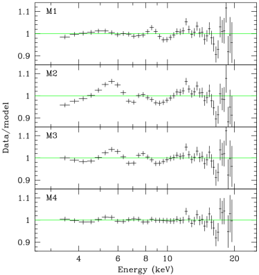
Figure 3: Residuals (data/model) for spectrum 7 (Table 1) fit with different models as summarized in Table 2. M4 is the most complex, but is the only physically motivated model which can fit this spectrum.

In the next step we replace the phenomenological description of the reflection features with the reflection code of Życki, Done & Smith (1998). This calculates the self-consistent line emission and reflected continuum from an ionized, relativistically smeared disc illuminated by a Comptonized continuum. We fix the iron abundance at 3 times solar (Lee et al. 2002). The model is parameterized by amplitude of reflection ($0\leq\Omega/2\pi\leq 2$), reflector ionization, $\xi$, and inner disc radius ($6\leq R_{\rm in}/R_{g}\leq 1000$, where $R_{g}\equiv GM/c^{2}$). We call this model M2 (see Table 2). Fitting results in Table 4 show that the fit is generally adequate except for S7 again, but the $\chi^{2}$ is always worse than for the simple model M1 fits. The physical description of the line and reflection features allows less freedom to fit the spectrum than the phenomenological components, and shows that there is more spectral complexity in the data (predominantly in S7) than is described by reflection.

Obs.	$kT_{\rm disc}$	$\Gamma$	$kT_{\rm comp}$	$\Omega/2\pi$	$\log(\xi)$	$R_{\rm in}$	$L_{\rm disc}$	$L_{\rm comp}$	$\chi^{2}/\nu$
	(keV)		(keV)		(erg cm s-1)	($R_{g}$)	($10^{38}$ erg s-1)
1	$<0.62$	$2.07_{-0.04}^{+0.02}$	$>18$	$0.15\pm 0.04$	$3.7_{-0.5}^{+0.2}$	$43_{-20}^{+80}$	$<1.8$	$5.3_{-0.6}^{+0.9}$	31.1/37
2	$0.91\pm 0.09$	$2.30\pm 0.02$	$>17$	$0.17_{-0.04}^{+0.14}$	$4.0_{-0.7}^{+0.6}$	$43_{-23}^{+75}$	$3.36_{-0.13}^{+0.15}$	$4.0_{-0.2}^{+0.4}$	28.9/37
3	$1.96\pm 0.25$	$1.61_{-0.47}^{+0.23}$	$4.2_{-0.4}^{+0.6}$	$>1.26$	$<2.6$	$41_{-14}^{+40}$	$5.2_{-1.1}^{+0.4}$	$1.7_{-0.3}^{+1.3}$	21.0/37
4	$0.80_{-0.24}^{+0.31}$	$2.35_{-0.16}^{+0.05}$	$6.4\pm 0.7$	$0.18_{-0.02}^{+0.04}$	$3.4_{-0.4}^{+0.3}$	$>100$	$<4.5$	$5.6_{-1.5}^{+3.0}$	46.6/37
5	$0.79_{-0.31}^{+0.12}$	$2.48_{-0.04}^{+0.08}$	$>6.2$	$0.18_{-0.02}^{+0.04}$	$3.4^{+0.3}_{-1.4}$	$>100$	$<5.6$	$5.6_{-0.7}^{+3.3}$	34.5/37
6	$0.94_{-0.02}^{+0.04}$	$3.03_{-0.07}^{+0.10}$	$3.53_{-0.17}^{+0.11}$	$0.50_{-0.11}^{+0.16}$	$<1.9$	$40_{-24}^{+230}$	$<1.9$	$10.7_{-0.9}^{+1.0}$	16.8/37
7	$1.17_{-0.06}^{+0.03}$	$1.5^{+0.5}_{-0.3}$	$2.58^{+0.30}_{-0.15}$	$1.40_{-0.22}^{+0.19}$	$3.6_{-0.2}^{+0.1}$	$>350$	$6.8_{-0.3}^{+0.2}$	$0.5_{-0.1}^{+0.3}$	208/37

Table 4: Best-fitting parameters for the selected spectra using a model with relativistically smeared, ionized reflection (M2 in Table 2).

Fig. 3 (panel M2) shows the residuals for the reflection model of S7, where the main mismatch is a marked excess in the data at $\sim$5.5 keV. This feature is systematically present in the other 6 spectra also, but is much less significant. While such features are obviously indicative of a strongly redshifted, broad shoulder to the iron line emission, these effects are already included in our model spectra (which has iron at 3$\times$ solar abundance, so the line is extremely strong). Instead this most probably represents the effects of excess absorption. Individual edges from neutral elements can be resolved with the Chandra grating spectra, and these clearly show that the neutral absorption has strong abundance anomalies, with Si and Fe being a factor 3.5 and 2.3 overabundant, respectively (Lee et al. 2002). This most probably arises from material ejected during the formation of the black hole (Lee et al. 2002), so it should be fairly far from the system, and constant with time. We use the varabs code to model this, fixing the column of all the elements at $4.7\times 10^{22}$ cm^-2 except for Si and Fe which are fixed at $16.4$ and $10.9\times 10^{22}$ cm^-2 respectively as measured by Chandra (Lee et al. 2002). We call this model M3 (Table 2).

We do not tabulate the detailed results of this intermediate model and only note that the increased absorption improves the fit for no increase in the number of degrees of freedom for all the data except S3. While $\chi^{2}/\nu$ = 34/37 for S3 is somewhat worse than that for the standard abundance model, it is an adequate fit to the data. However, S7 still has an unacceptable $\chi^{2}/\nu=93/37$, as shown by its residuals in Fig. 3 (panel M3).

High- and moderate-resolution spectral data indicate yet more complexity in the absorption, in that as well as the anomalous abundance neutral absorption there is clear evidence for ionized absorption. Both ASCA and Chandra detect resonance line absorption from highly ionized iron, and show that this is variable with time and/or spectral state of GRS 1915+105 (Kotani et al. 2000; Lee et al. 2002). We model this by narrow Gaussian lines corresponding to He- and H-like iron, with K$\alpha$ transitions at 6.67 and 6.9 keV, respectively. We also include the (fixed energy) K$\beta$ and $\gamma$ lines at $7.80,8.21$ keV for He-like and $8.16,8.61$ keV for H-like, with fixed relative intensity to the K$\alpha$ transition of 0.07 and 0.06 for He-like and 0.2 and 0.07 for H-like (Kotani et al. 2000). Thus there are only two additional free parameters, which are the intensities of the 6.67 and 6.90 keV absorption lines, denoted as $I_{6.67}$ and $I_{6.90}$, respectively. These are not strongly detected in S1–6, but the fit to S7 is significantly improved, and now gives an acceptable $\chi^{2}/\nu=34.2/35$. Residuals to this fit are shown in Fig. 3 (panel M4).

We use the xstar code (Kallman et al. 1996) to check the assumption that the dominant opacity is from the iron absorption lines (as opposed to lines from other elements and/or photoelectric edges). We assume the same Si/Fe abundance anomalies as in the neutral absorption, illuminated with a $\Gamma=2$ power law. This self-consistent absorption model gives an identical $\chi^{2}$ to that of the resonance absorption lines model of Table 5. The resulting parameters imply these lines arise in an equivalent hydrogen column of $\sim 3\times 10^{23}$ cm^-2 with ionization parameter $\xi\sim 10^{3.7}$ ergs cm s^-1. None of the seven spectra are significantly better fit with the full xstar ionized absorption models so we use the absorption lines in all subsequent fits as they are easier to constrain.

Our final model M4 consists of the disc emission, its thermal Comptonization, ionized and relativistically smeared reflection, cold absorption with anomalous abundance of silicon and iron and resonance absorption lines from highly ionized iron. The fit results to all the seven spectra are in Table 5.

The effective increase in cold absorption affected mostly the soft part of the spectrum, decreasing the soft colour by $\sim$0.2, when M2 was replaced by M4. The extrapolated bolometric disc luminosity is also heavily dependent on the assumed absorption model. With model M4 the disc luminosity is significantly larger than with M2. This is particularly well seen for spectrum S3, where changing the absorption model has switched the fit from a high disc temperature ($\approx$ 2 keV), low Comptonized luminosity model, to a low disc temperature ($\approx$ 0.7 keV), high Comptonized luminosity model. In S6 the best-fitting M4 model is disc-dominated ($\sim$0.1 of total power in the Comptonized tail), though this particular fit is very poorly constrained and a more Comptonized spectrum ($\sim$0.6 luminosity in the tail) is also possible. This shows the difficulties in dealing with such an absorbed source, and illustrates the reason for the conservative limit of DG03 of restricting their sample to objects with column of $<2\times 10^{22}$ cm^-2.

We note that none of the models including reflection (M2–4) give any indication for the extreme relativistically smeared components expected for an X-ray illuminated disc which extends down to the last stable orbit around a black hole. All the inner radii derived from relativistic smearing are substantially larger than $\sim$20 $R_{g}$ (10 Schwarzchild radii). Similarly large radii are also inferred by Martocchia et al. (2002) from BeppoSAX data on this source. This is important as there is some evidence that GRS 1915+105 is an extreme Kerr black hole (Zhang et al. 1997; Cui et al. 1998; Sobolewska & Życki 2003), with the disc extending down to 1.24 $R_{g}$. However, the line broadening does not rule out such a disc since the reflector is highly ionized. The innermost disc may well be so highly ionized that iron in the disc is completely stripped, so there are no line features produced in the most strongly curved space-time regions though there can be continuum emission/reflection from the disc (see also Wilson & Done 2001 for a similar conclusion for the very high state spectra of XTE J1550–564).

Obs.	$kT_{\rm disc}$	$\Gamma$	$kT_{\rm comp}$	$\Omega/2\pi$	$\log(\xi)$	$R_{\rm in}$	$I_{6.67}$	$I_{6.95}$	$L_{\rm disc}$	$L_{\rm comp}$	$\chi^{2}/\nu$
	(keV)		(keV)		(erg cm s-1)	($R_{g}$)	($10^{-3}$ cm-2 s-1)		($10^{38}$ erg s-1)
1	$<0.45$	$2.07\pm 0.03$	$>12$	$0.20\pm 0.03$	$3.8_{-0.5}^{+0.6}$	$11\pm 3$	$<1.6$	$<3.7$	$10.9_{-3.6}^{+1.6}$	$4.9_{-0.4}^{+1.1}$	26.4/35
2	$0.55^{+0.11}_{-0.10}$	$2.37^{+0.02}_{-0.06}$	$>25$	$0.34_{-0.08}^{+0.24}$	$4.3\pm 0.5$	$18_{-4}^{+10}$	$<3.0$	$7.1^{+5.1}_{-2.3}$	$6.8_{-0.6}^{+2.6}$	$5.0_{-0.7}^{+1.3}$	15.2/35
3	$0.70_{-0.16}^{+0.17}$	$2.11\pm 0.05$	$5.54_{-0.37}^{+0.44}$	$0.23^{+0.07}_{-0.03}$	$3.3\pm 0.4$	$25_{-7}^{+15}$	$<3.5$	$<8.3$	$<2.2$	$6.0_{-0.1}^{+0.3}$	33.7/35
4	$<0.47$	$2.30\pm 0.04$	$5.53_{-0.33}^{+0.41}$	$0.25_{-0.04}^{+0.06}$	$3.5_{-0.5}^{+0.4}$	$34_{-12}^{+30}$	$<5.3$	$<12.4$	$12.5_{-5.9}^{+5.7}$	$8.7_{-0.3}^{+0.7}$	38.3/35
5	$<0.47$	$2.51_{-0.05}^{+0.04}$	$6.55_{-0.53}^{+0.63}$	$0.23\pm 0.06$	$3.5\pm 0.5$	$45_{-19}^{+71}$	$<7.7$	$<13.1$	$20.9_{-7.7}^{+6.9}$	$10.2_{-0.3}^{+0.8}$	18.9/35
6	$1.61_{-0.61}^{+0.08}$	$<2.85$	$2.78_{-0.08}^{+0.52}$	$>0.12$	$4.9_{-2.7}^{+0.3}$	$*$	$*$	$<18$	$16.2_{-9.8}^{+0.9}$	$1.2_{-0.5}^{+8.0}$	9.8/35
7	$0.99_{-0.05}^{+0.07}$	$1.93_{-0.20}^{+0.41}$	$2.43_{-0.08}^{+0.14}$	$1.88_{-0.38}^{+0.12}$	$3.3\pm 0.3$	$>150$	$22^{+9}_{-13}$	$14^{+7}_{-6}$	$7.9_{-0.4}^{+0.3}$	$0.9_{-0.2}^{+0.6}$	34.2/35

Table 5: Best-fitting parameters for the selected spectra (Table 1) using our best physical model with reflection, anomalous neutral abundances and ionized iron absorption lines (M4 in Table 2). An asterisk indicates that the parameter is completely unconstrained.

3.4 Physical model applied to all pointed spectra

The previous section has shown that a physically motivated model for GRS 1915+105 which can adequately describe all the selected spectra includes anomalous abundance neutral absorption, ionized absorption, relativistically smeared, ionized reflection, with continuum from the disc and thermal Comptonization. The high absorption means that the derived soft colour and disc luminosity change substantially with changing the model. Nonetheless, we now have a physical model which incorporates all the observed spectral features so we can at least use this to get our best estimate for the intrinsic colours of the system. We refit the 292 spectra from Fig. 2 with this physical model, and the resulting colour-colour diagram is shown in Fig. 4. Black and blue points on this diagram correspond to spectra which show little variability, so the model parameters represent the physical components of the spectra. However, this is not the case for the spectra averaged over high-variability periods (shown in green and red in Figs. 2 and 4), where the physical model is merely parameterizing the time averaged spectrum to give a best estimate for the colours. A comparison with Fig. 2 confirms the result from the individual spectral fits that the major change is that the soft colour is reduced by $\sim$0.2 in all spectra, so that the overall pattern stays the same.

Fig. 4 also shows the best-fitting unfolded individual spectra, together with the model components. Spectra along the upper diagonal branch between S1 and S2 have a hard component which has no discernable rollover in the PCA bandpass ($kT_{\rm comp}\ga 10$ keV), with spectral index steepening from S1 to S2. S3–S5 form a parallel diagonal track for changing spectral index, but here the electron temperature is clearly seen in the high-energy spectral curvature ($kT_{\rm comp}\sim 6$ keV). All these spectra have comparable disc and hard tail luminosity. S6 and S7 are different from S1–S5 in that there is an increase in disc temperature. The hard tail is characterized by even lower temperature electrons, $kT_{\rm comp}\sim$ 2–3 keV. The disc temperature $\ga$1 keV rather than hard tail dominates the change in soft colour.

Only spectra with colours similar to those of S7 show a strong detection of the resonance absorption lines from He- and H-like Fe. This is consistent with previous moderate- and high-resolution spectra from ASCA and Chandra. The Chandra spectrum of Lee et al. (2002) has a continuum similar to S2, with resonant line intensities of a few $10^{-3}$ photons cm^-2 s^-1, easily consistent with our upper limit in Table 5. The three ASCA spectra of Kotani et al. (2000) taken in 1994 September, 1995 April and 1996 October, have colours similar to S7, midway between S6 and S7, and similar to S5, respectively. The lines are only significantly detected in the 1994 and 1995 ASCA data, where they have equivalent widths of 30–50 eV for the He- and H-like K$\alpha$ lines. This is somewhat smaller than, but comparable to the 100–120 eV equivalent widths for these lines we derive for S7. This material is almost certainly part of an outflowing wind, which can have a comparable mass loss rate to that of the mass accretion rate required to power the observed emission (Lee et al. 2002). That the lines are most visible in S7 can be explained as an ionization effect. All the other spectra are harder, so a higher proportion of iron can be completely ionized, giving smaller equivalent width features. This can also feedback onto the wind acceleration mechanism if there is considerable line driving, so that there is intrinsically less wind at higher ionization (e.g. Proga & Kallman 2002).

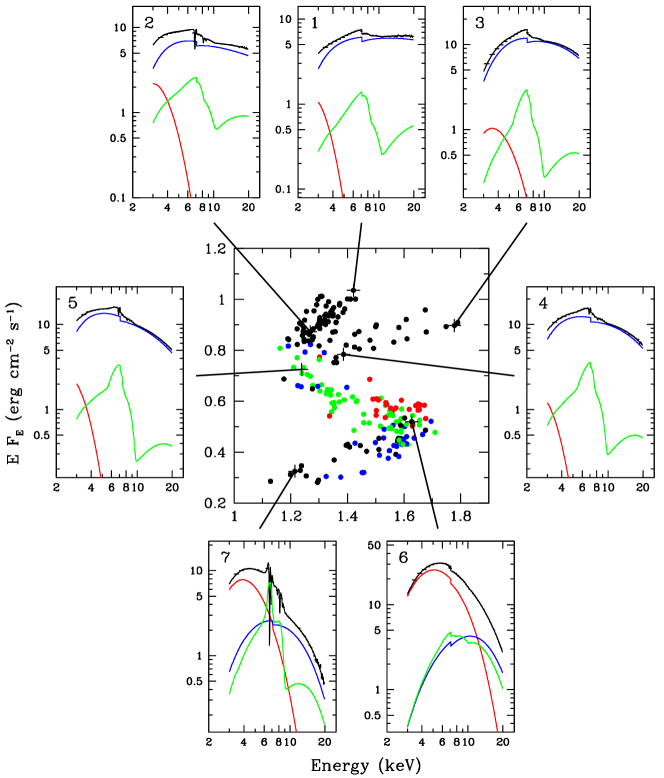
Figure 4: The intrinsic colour-colour plot for all the observations shown in Fig. 2 fitted with the physical model including reflection, anomalous neutral abundances and ionized iron absorption lines (M4, Table 2). The individual spectra corresponding to the selected observations listed in Table 1 are shown deconvolved with this model, where the red, blue and green lines give the disc, Comptonized emission and its reflection, respectively. The best-fitting parameters for each spectrum are shown in Table 5.

4 GRS 1915+105 in context

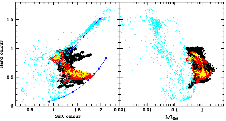
Figure 5: The intrinsic colour-colour (left) and colour-luminosity (right) diagrams for GRS 1915+105 created from 128-s spectra. Black, red and yellow points denote periods of low, high and very high variability with r.m.s. $<$ 40, 40–60 and $\geq$ 60 per cent, respectively. On top of this we have superimposed the data from ‘normal’ black holes (cyan points) from DG03 and GD03. The blue lines on the left diagram show the model colours of a power law (upper line, with $\Gamma$ increasing from 1.5 to 3.0 diagonally downwards) and a multicolour disc (lower line, with $kT_{\rm disc}$ increasing from 1 to 3 keV rightwards). The yellow points track the highest variability of GRS 1915+105, related to limit-cycle instability. It occurs between colours corresponding to the very high state (1.1, 0.8) and a hot ultrasoft state corresponding to an effective disc temperature of excess of 2 keV.

While our physically based models give generally good fits to all the individual observation ID spectra, these data are extracted from full RXTE pointings. These have exposure times of several kiloseconds, so many of them average over periods of strong spectral variability. Thus the parameters derived from the spectral fits in Fig. 4 will not show the extremes of luminosity, and can be misleading since the model components are not linear.

Thus we need to go back to the 128-s spectra in order to get a clearer idea of the properties of GRS 1915+105. However, it is not feasible to fit all 16489 spectra with the computationally intensive physical model, where a single fit can take tens of minutes. Fortunately, the spectral fits from Section 3.3 show that most of the change in derived soft colour and soft luminosity between the simple phenomenological description and the more physical model arises from the change in cold absorption. Yet most of the increase in fitting time comes from modelling reflection. Hence we use the simple phenomenological model of smeared edge and broad line to describe reflection (as in model M1 of Table 2), with fixed anomalous abundances of Si and Fe to test how well this can reproduce the colours and luminosities derived from the physical model (we call this model M5; see Table 2). A fit of this simple model to the seven selected spectra from Section 3.3 shows that it gives a very good match to the colours from the physical model, and reproduces the soft luminosities to within a factor of $\sim$2. This gives some measure of the systematic uncertainty in deriving the total (model dependent) luminosity.

We use this simplified model (M5) to fit all the 128-s spectra. The left panel in Fig. 5 shows the colour-colour plot derived from this (black, red and yellow points), compared to the colours derived from the ‘normal’ black holes of DG03 and GD03 (cyan points). DG03 show how position on this diagram relates to the different black hole spectral states (see e.g. the reviews by Tanaka & Lewin 1995; Esin, Mclintock & Narayan 1997), which we briefly summarize here. The power law dominated low/hard state corresponds to the diagonal track starting from colours (2.0, 1.5) for an photon spectral index of $\Gamma\sim 1.5$, extending down to about (1.5, 1.0) as the spectrum softens to $\Gamma\sim 2$. Intermediate or very high state spectra have roughly equal luminosity in a disc component as in a fairly steep ($\Gamma\sim$ 2–2.5) power-law tail and have colours within $\sim$0.2 of (1.3, 0.8). The disc is completely dominant in the ultrasoft state, so the colours are close to those predicted by the pure disc blackbody track. The classic high/soft state (as seen e.g. in Cyg X-1: Gierliński et al. 1999) has a disc-dominated soft spectrum but at higher energies has a noticeable fraction of luminosity in a power-law tail. This gives it somewhat harder colours than the ultrasoft states at $\sim$(0.7, 0.8). This is the region identified by DG03 as a sufficient (but not necessary) condition for the object to be a black hole.

The spectra from GRS 1915+105 with colours similar to S1–S5 overlap with the intermediate/very high state region on the colour-colour diagram, while S6 and S7 occupy the high-temperature end of the ultrasoft region. GRS 1915+105 never goes into the classic low/hard state $\sim$(2.0, 1.5), nor does it go into the ‘black hole only’ region of DG03 (the classic high/soft state).

We categorize each 128-s spectra according to variability of a period they come from, marking them in black, red and yellow for r.m.s. $<$ 40, 40–60 and $\geq$ 60 per cent, respectively. This makes it clear that the major instability track is between spectra with colours like S2 and S6 (see Fig. 2). A comparison with Fig. 4 shows that the higher time resolution of these spectra (128-s as opposed to a few ks) gives a similar diagonal track for the limit cycle, but extending further towards the disc blackbody line (i.e. corresponding to higher temperatures and luminosities). With even higher resolution data then this track extends even further (see the solid and dashed line in Fig. 1a), showing that our 128-s spectra do not follow the fastest variability of GRS 1915+105.

The upper-left end of the track corresponds to spectral state C (Fig. 1b), rather misleadingly also called the hard state. In fact, it is very similar to e.g. very high state data from XTE J1550–564 (Gierliński & Done 2003a). There is nothing special in the spectral shape here which hints at the origin of the unique variability of GRS 1915+105. The other end of the instability track lays in the ultrasoft region, corresponding predominantly to the higher temperature state B (Fig. 1b). These have similar colours to pure disc spectra, but are at a higher effective temperature than any of the other black holes. Thus the only hint of difference in the colours for the origin of the dramatic instability in GRS 1915+105 is that the ultrasoft state appears to extend to higher disc temperatures.

The right panel of Fig. 5 is a colour-luminosity plot for GRS 1915+105 superimposed on that for all the other black holes (DG03, GD03). The colour-coding is the same as in the left panel. This is much more illuminating as to the origin of the unique instability behaviour of GRS 1915+105. Here it is plain that the instability occurs in the most luminous spectra, those which have $L>L_{\rm Edd}$, and only GRS 1915+105 goes up to such high luminosities. The luminosity never drops below $\sim$0.3 $L_{\rm Edd}$, explaining why GRS 1915+105 never goes into the hard state (typically seen only at luminosities lower than a few percent of Eddington). It also explains why GRS 1915+105 never goes into the ‘black hole only’ area of the colour-colour diagram. Spectra in this region, characterized by a low-temperature disc component together with a weak hard tail, are seen predominantly around $\sim$0.1 $L_{\rm Edd}$. The persistently high luminosity of GRS 1915+105 takes it above these low disc temperatures.

Where GRS 1915+105 has a luminosity which overlaps with that of the ‘normal’ black holes it shows comparable spectra and does not show the dramatic limit cycle variability. However, it also extends to higher luminosities, up to $\sim$2–3 $L_{\rm Edd}$. This makes it unique among the black holes studied by DG03 and GD03, and it is here that the unique instability occurs. However, supereddington luminosity seems to be only a necessary, not sufficient condition for the disc instability. There are several low variability spectra from GRS 1915+105 which exceed the Eddington limit. Perhaps the instability requires that the disc as opposed to total luminosity goes above Eddington, or perhaps this merely shows that the disc structure takes some time to respond to an increase in central mass accretion rate (e.g. van der Klis 2001).

The left panel in Fig. 5 includes the background colour tracks for a disc blackbody spectrum, and the high luminosity, ultrasoft spectra on the extreme end of the limit-cycle variability intersect this line at colours corresponding to $kT_{\rm disc}\sim 2.2$ keV. A more detailed analysis is complicated as many of these most extreme colour 128-s spectra still average over substantial variability. However, these ultrasoft spectra have similar colours to the stable spectrum S6. If they are truly similar then the results in Table 5 indicate that these are not simply high-temperature disc emission. Instead they might be much better fit by a lower temperature disc at $\la$1.6 keV, with a fairly strong ($\ga$10 per cent of bolometric flux), low temperature (few keV) Comptonized tail (see also Zdziarski et al. 2001). A similar effect is also seen in the high-temperature ultrasoft spectra of GRO J1655–40 (Kubota, Makishima & Ebisawa 2001; GD03).

However, irrespective of the detailed spectral form of the highest luminosity spectra, we include the minimum absorption column, so derive (on average) a lower limit to the flux. Additional, time variable cold absorption components (e.g. Sobolewska & Życki 2003) will only increase the inferred luminosity. There is a factor $\sim$2 systematic uncertainty on the distance (7–12 kpc: Fender et al. 1999, though the lower limit could present significant problems for the derived luminosity of the companion star: Greiner et al 2001b) so this could reduce the bolometric luminosity estimates by at most a factor 4. Thus it seems that the trigger for the characteristic limit-cycle variability in GRS 1915+105 is almost certainly super-Eddington accretion rates.

5 Limit-cycle variability

GRS 1915+105 is the most luminous black hole system studied here, and is also the only one to show the characteristic limit-cycle variability. Plainly the results are consistent with the accretion flow onto a black hole becoming unstable at very high luminosities of $\ga L_{\rm Edd}$. The same instability does not seem to operate in neutron stars. Z sources emit at 1–3 $L_{\rm Edd}$, while Cir X-1 can reach up to $10L_{\rm Edd}$ (DG03). Approximately half of the neutron star luminosity should be from the boundary layer, so the accretion flow luminosity is only $\sim$0.5–1.5 $L_{\rm Edd}$ in the Z sources, perhaps too low to trigger the instability (but not in Cir X-1). Alternatively, irradiation of the accretion flow by the boundary layer may act as a stabilizing mechanism (Czerny, Czerny & Grindlay 1986, but see Mineshige & Kusenose 1993 and below).

Following Belloni et al. (1997a, b), the instability itself is generally associated with the well known radiation pressure instability of a standard $\alpha$ disc at high luminosities (Lightman & Eardley 1974; Shakura & Sunyaev 1976). In its simplest form this predicts that the inner accretion flow cycles between a highly luminous, hot, advection-dominated disc and a much lower luminosity, cooler, gas pressure-dominated disc (Abramowicz et al. 1988; Honma, Matsumoto & Kato 1991; Szuszkiewicz & Miller 1997, 1998; Zampieri, Turolla & Szuszkiewicz 2001). One key problem with this interpretation is that the limit-cycle variability should occur at well below $L_{\rm Edd}$ (see Nayakshin, Rappaport & Melia 2000 for other problems). Theoretical models show that the limit cycles become noticeable at $L_{\rm disc}\ga 0.3L_{\rm Edd}$ (Janiuk, Czerny & Siemiginowska 2002), yet none of the comparison sample of ‘normal’ black holes above this luminosity show the limit cycle (Kubota et al. 2001; Kubota & Makishima 2003; GD03).

GD03 summarize various ways to delay the onset of the radiation pressure instability in a standard disc. Generally these involve some additional energy loss channel e.g. dissipating some of the accretion energy in a hard X-ray corona, or via a wind or jet. The problem with these is that the ‘normal’ black holes can show disc-dominated spectra (so no obvious energy loss in a corona/jet) without producing the instability even at $L_{\rm disc}\sim 0.5L_{\rm Edd}$ (GD03). By contrast GRS 1915+105 shows strong coronal emission and has a jet and a wind, all of which should act to stabilize the disc, yet does show the instability. Irradiation of the disc by the strong coronal emission should also act as a stabilizing mechanism, similarly to that proposed for the boundary layer in neutron stars (Czerny et al. 1986). Thus it seems unlikely that irradiation alone can stabilize the disc in the Z sources since it does not manage to stabilize GRS 1915+105.

The ‘normal’ black holes show that the disc is stable up to at least $L_{\rm disc}\sim 0.5L_{\rm Edd}$, so its structure must be rather different from that predicted by the standard $\alpha$ disc equations (GD03). The fact that the instability in GRS 1915+105 is triggered at or near Eddington luminosity seems to suggest that radiation pressure does play a pivotal role in the formation of the dramatic variability. That the $\alpha$ disc equations do not work in detail is perhaps not surprising given the ad hoc nature of viscous heating in these models. The next generation of disc models will give a much better estimate for the disc structure, as these can incorporate the MHD dynamo which is the physical origin of the viscosity (Balbus & Hawley 1991). When these models are sufficiently developed to solve the time dependent 3D, coupled radiation and magneto-hydrodynamic equations over a substantial range of radii (Turner, Stone & Sano 2002; Turner et al. 2003) then the question of inner disc stability for highly luminous systems can be revisited.

6 Long-term variability

The unique short-term limit-cycle variability of GRS 1915+105 is plausibly because it reaches higher $L/L_{\rm Edd}$ than any other known Galactic black hole. But then the question becomes why GRS 1915+105 alone reaches such high luminosities? The answer to this lies in the evolutionary state of GRS 1915+105. The system has the longest known period of any LMXB of 33.5 days, implying a very wide orbit (Greiner et al. 2001a). The secondary is a low-mass giant star (Greiner et al. 2001b), so the accretion takes place via Roche lobe overflow (Eikenberry & Bandyopadhyay 2000).

There is now considerable agreement that transient outbursts in the LMXBs are caused by the classic disc instability mechanism which operates when hydrogen goes from being mainly neutral to mainly ionized. This is a very different physical mechanism for a disc instability than the radiation pressure instability discussed above, and happens at much lower luminosity, but it gives rise to another S-shaped thermal equilibrium curve (Smak 1982). In discs around white dwarfs it can trigger limit cycles where there are disc outbursts on timescales of days–weeks, followed by a period of quiescence lasting weeks–months (see e.g. the review by Osaki 1996). In LMXBs the disc structure is strongly modified by irradiation once the outburst starts, keeping hydrogen ionized for much longer so that the outburst timescales are dramatically extended (van Paradijs 1996; King 1997; King & Ritter 1998; Dubus et al. 2001).

The peak luminosity at the start of the LMXB outburst is determined by the disc size, $R_{T}$. The maximum mass the disc can hold before going into outburst is $\propto R_{T}^{3}$, while the inflow timescale is $\propto R_{T}$. Thus the peak luminosity $\propto R^{2}_{T}$ so the bigger the disc, the bigger the peak luminosity (King & Ritter 1998). But the disc size in LMXB is fixed by tidal torques to $\sim$1.4$\times R_{\rm circ}$, where $R_{\rm circ}$ is the circularization radius of the binary (Shahbaz, Charles & King 1998), and the binary system parameters are determined by the requirement that the secondary star can overflow its Roche lobe. For main sequence secondaries the orbit must be fairly small, so the disc is small. GRS 1915+105 has a giant secondary, so has a huge disc, with $R_{T}\sim 10^{12}$ cm for a mass ratio of $0.1$ (e.g. Frank, King & Raine 1992). The quiescent disc mass is $\sim$10²⁸ g (Shahbaz, Charles & King 1998), which can maintain an Eddington accretion rate for $\sim$10 years, similar to observed outburst timescale.

Thus both the long and short-term unique variability behaviour of GRS 1915+105 can be explained as a function of its evolutionary state, where the wide orbit allows a huge disc to form.

7 Conclusions

GRS 1915+105 is not in a separate class from ‘normal’ black holes. When it is at the same $L/L_{\rm Edd}$ then its spectra and (more importantly) time variability behaviour are similar to that seen in the ’normal’ black holes. Its unique limit cycle variability only appears when it radiates at uniquely high (super Eddington) luminosities.

GRS 1915+105 boldly goes to luminosities where no black hole has gone before, and we eagerly await the next generation of disc models which will more clearly identify the origin of the instability.

References

- [\citeauthoryearAbramowicz et al.1988] Abramowicz M. A., Czerny B., Lasota J. P., Szuszkiewicz E., 1988, ApJ, 332, 646
- [\citeauthoryearAnders & Ebihara1982] Anders E., Ebihara M., 1982, GeCoA, 46, 2363
- [] Arnaud K. A., 1996, in Jacoby G. H., Barnes J., eds., Astronomical Data Analysis Software and Systems V. ASP Conf. Series Vol. 101, San Francisco, p. 17
- [\citeauthoryearBailyn et al.1998] Bailyn C. D., Jain R. K., Coppi P., Orosz J. A., 1998, ApJ, 499, 367
- [\citeauthoryearBalbus & Hawley1991] Balbus S. A., Hawley J. F., 1991, ApJ, 376, 214
- [\citeauthoryearBelloni et al.1997] Belloni T., Méndez M., King A. R., van der Klis M., van Paradijs J., 1997a, ApJ, 479, L145
- [\citeauthoryearBelloni et al.1997] Belloni T., Méndez M., King A. R., van der Klis M., van Paradijs J., 1997b, ApJ, 488, L109
- [\citeauthoryearBelloni et al.2000] Belloni T., Klein-Wolt M., Méndez M., van der Klis M., van Paradijs J., 2000, A&A, 355, 271, B00
- [\citeauthoryearCastro-Tirado, Brandt, & Lund1992] Castro-Tirado A. J., Brandt S., Lund N., 1992, IAUC, 5590, 2
- [\citeauthoryearChaty et al.1996] Chaty S., Mirabel I. F., Duc P. A., Wink J. E., Rodríguez L. F., 1996, A&A, 310, 825
- [\citeauthoryearChen et al.1995] Chen X., Abramowicz M. A., Lasota J., Narayan R., Yi I., 1995, ApJ, 443, L61
- [\citeauthoryearChen, Swank, & Taam1997] Chen X., Swank J. H., Taam R. E., 1997, ApJ, 477, L41
- [\citeauthoryearCui, Zhang, & Chen1998] Cui W., Zhang S. N., Chen W., 1998, ApJ, 492, L53
- [\citeauthoryearCzerny, Czerny, & Grindlay1986] Czerny B., Czerny M., Grindlay J. E., 1986, ApJ, 311, 241
- [Di Salvo, Méndez, & van der Klis(2003)] Di Salvo, T., Méndez, M., & van der Klis, M. 2003, A&A, 406, 177
- [\citeauthoryearDone & Gierliński2003] Done C., Gierliński M., 2003, MNRAS, 342, 1041, DG03
- [\citeauthoryearDubus, Hameury, & Lasota2001] Dubus G., Hameury J.-M., Lasota J.-P., 2001, A&A, 373, 251
- [\citeauthoryearEbisawa1991] Ebisawa K., 1991, PhD Thesis
- [\citeauthoryearEikenberry & Bandyopadhyay2000] Eikenberry S. S., Bandyopadhyay R. M., 2000, ApJ, 545, L131
- [\citeauthoryearEikenberry et al.1998] Eikenberry S. S., Matthews K., Morgan E. H., Remillard R. A., Nelson R. W., 1998, ApJ, 494, L61
- [\citeauthoryearEsin, McClintock, & Narayan1997] Esin A. A., McClintock J. E., Narayan R., 1997, ApJ, 489, 865
- [\citeauthoryearEsin, Lasota, & Hynes2000] Esin A. A., Lasota J.-P., Hynes R. I., 2000, A&A, 354, 987
- [\citeauthoryearFender & Kuulkers2001] Fender R. P., Kuulkers E., 2001, MNRAS, 324, 923
- [Fender et al.(1999)] Fender, R. P., Garrington, S. T., McKay, D. J., Muxlow, T. W. B., Pooley, G. G., Spencer, R. E., Stirling, A. M., & Waltman, E. B. 1999, MNRAS, 304, 865
- [] Frank J., King A., Raine D., 1992, Accretion Power in Astrophysics, Cambridge University Press
- [\citeauthoryearGierliński & Done2003] Gierliński M., Done C., 2003a, MNRAS, 342, 1083
- [] Gierliński M., Done C., 2003b, MNRAS, submitted (astro-ph/0307333), GD03
- [\citeauthoryearGreiner, Morgan, & Remillard1996] Greiner J., Morgan E. H., Remillard R. A., 1996, ApJ, 473, L107
- [\citeauthoryearGreiner, Cuby, & McCaughrean2001] Greiner J., Cuby J. G., McCaughrean M. J., 2001a, Nat, 414, 522
- [\citeauthoryearGreiner et al.2001] Greiner J., Cuby J. G., McCaughrean M. J., Castro-Tirado A. J., Mennickent R. E., 2001b, A&A, 373, L37
- [\citeauthoryearHonma, Kato, & Matsumoto1991] Honma F., Matsumoto R., Kato S., 1991, PASJ, 43, 147
- [\citeauthoryearJaniuk, Czerny, & Siemiginowska2002] Janiuk A., Czerny B., Siemiginowska A., 2002, ApJ, 576, 908
- [\citeauthoryearKallman et al.1996] Kallman T. R., Liedahl D., Osterheld A., Goldstein W., Kahn S., 1996, ApJ, 465, 994
- [\citeauthoryearKing1997] King A. R., 1997, MNRAS, 288, L16
- [\citeauthoryearKing & Ritter1998] King A. R., Ritter H., 1998, MNRAS, 293, L42
- [\citeauthoryearKotani et al.2000] Kotani T., Ebisawa K., Dotani T., Inoue H., Nagase F., Tanaka Y., Ueda Y., 2000, ApJ, 539, 413
- [\citeauthoryearKubota, Makishima, & Ebisawa2001] Kubota A., Makishima K., Ebisawa K., 2001, ApJ, 560, L147
- [] Kubota A., Makishima K., 2003, ApJ, submitted
- [\citeauthoryearLee et al.2002] Lee J. C., Reynolds C. S., Remillard R., Schulz N. S., Blackman E. G., Fabian A. C., 2002, ApJ, 567, 1102
- [\citeauthoryearLightman & Eardley1974] Lightman A. P., Eardley D. M., 1974, ApJ, 187, L1
- [\citeauthoryearMartocchia et al.2002] Martocchia A., Matt G., Karas V., Belloni T., Feroci M., 2002, A&A, 387, 215
- [\citeauthoryearMineshige & Kusunose1993] Mineshige S., Kusunose M., 1993, PASJ, 45, 113
- [\citeauthoryearMirabel & Rodriguez1994] Mirabel I. F., Rodríguez L. F., 1994, Nat, 371, 46
- [\citeauthoryearMirabel & Rodríguez1999] Mirabel I. F., Rodríguez L. F., 1999, ARA&A, 37, 409
- [\citeauthoryearMitsuda et al.1984] Mitsuda K. et al., 1984, PASJ, 36, 741
- [Morgan, Remillard, & Greiner(1997)] Morgan, E. H., Remillard, R. A., & Greiner, J. 1997, ApJ, 482, 993
- [\citeauthoryearNayakshin, Rappaport, & Melia2000] Nayakshin S., Rappaport S., Melia F., 2000, ApJ, 535, 798
- [\citeauthoryearOsaki1996] Osaki Y., 1996, PASP, 108, 39
- [\citeauthoryearPooley & Fender1997] Pooley G. G., Fender R. P., 1997, MNRAS, 292, 925
- [\citeauthoryearProga & Kallman2002] Proga D., Kallman T. R., 2002, ApJ, 565, 455
- [\citeauthoryearShahbaz, Charles, & King1998] Shahbaz T., Charles P. A., King A. R., 1998, MNRAS, 301, 382
- [\citeauthoryearShakura & Sunyaev1973] Shakura N. I., Sunyaev R. A., 1973, A&A, 24, 337
- [\citeauthoryearShakura & Sunyaev1976] Shakura N. I., Sunyaev R. A., 1976, MNRAS, 175, 613
- [\citeauthoryearSmak1982] Smak J., 1982, AcA, 32, 199
- [\citeauthoryearSobolewska &Zdotycki2003] Sobolewska M. A., Życki P. T., 2003, A&A, 400, 553
- [\citeauthoryearSzuszkiewicz & Miller1997] Szuszkiewicz E., Miller J. C., 1997, MNRAS, 287, 165
- [\citeauthoryearSzuszkiewicz & Miller1998] Szuszkiewicz E., Miller J. C., 1998, MNRAS, 298, 888
- [] Tanaka Y., Lewin W. H. G. 1995, in X–Ray Binaries, ed. W. H. G. Lewin, J. van Paradijs & E. van den Heuvel (Cambridge: Cambridge Univ. Press), 126
- [Turner 2002] Turner N. J., Stone J. M., Sano T., 2002, ApJ, 566, 148
- [] Turner N. J., Stone J. M., Krolik J. H., Sano T., 2003, preprint (astro-ph/0304511)
- [\citeauthoryearWilson & Done2001] Wilson C. D., Done C., 2001, MNRAS, 325, 167
- [van der Klis(2001)] van der Klis, M. 2001, ApJ, 561, 943
- [\citeauthoryearvan Paradijs1996] van Paradijs J., 1996, ApJ, 464, L139
- [van Straaten, van der Klis, & Méndez(2003)] van Straaten, S., van der Klis, M., & Méndez, M. 2003, ApJ, 596, 1155
- [\citeauthoryearZampieri, Turolla, & Szuszkiewicz2001] Zampieri L., Turolla R., Szuszkiewicz E., 2001, MNRAS, 325, 1266
- [\citeauthoryearZdziarski, Johnson, & Magdziarz1996] Zdziarski A. A., Johnson W. N., Magdziarz P., 1996, MNRAS, 283, 193
- [\citeauthoryearZdziarski et al.2001] Zdziarski A. A., Grove J. E., Poutanen J., Rao A. R., Vadawale S. V., 2001, ApJ, 554, L45
- [\citeauthoryearZhang, Cui, & Chen1997] Zhang S. N., Cui W., Chen W., 1997, ApJ, 482, L155
- [\citeauthoryearZycki, Done, & Smith1998] Życki P. T., Done C., Smith D. A., 1998, ApJ, 496, L25