Optical and Near-IR Spectra of O-rich Mira Variables : a Comparison between Models and Observations

Pulsation models are crucial for the interpretation of spectrophotometric and interferometric observations of Mira variables. Comparing predicted and observed spectra is one way of establishing the validity of such models. In this paper, we focus on the models published between 1996 and 1998 by Bessell, Hofmann, Scholz and Wood. A few new model spectra are added, to improve available phase coverage. We compare the synthetic spectra with observed low resolution spectra of optically selected oxygen-rich Miras, over a range of optical and near-IR wavelengths that encompasses most of the stellar energy output. We investigate the overall energy distributions, and specific spectral features in the near-IR wavelength range. The agreement between the observed and the model-predicted properties is found to be reasonably good. However, there are discrepancies seen especially in various molecular bands.
We find that different combinations of stellar parameters and pulsation phases often result in very similar model spectra. Therefore the problem of deriving parameters of a Mira variable from its spectrum has no unique solution. More advanced models than presently available, providing even better fits to the data and covering a wider range of parameters, would be needed to achieve better discrimination.

1 Introduction

Mira variables play a major role in understanding stellar evolution and galactic spectral evolution. Stellar lifetimes, the contribution of AGB stars to the integrated light emission of stellar populations, or the chemical yields of intermediate mass stars depend critically on properties such as stellar mass, pulsation and mass loss. Hence, estimates of the fundamental stellar parameters and atmospheric properties of these stars, from spectroscopic, photometric and interferometric observations, remain crucial. The interpretation of any of these data relies on stellar models.

In a previous paper (Tej et al. 2003 = TLS03), based on models of Bessell et al. (1996 = BSW96) and Hofmann et al. (1998 = HSW98), we have shown that simultaneous spectrophotometric observations of absorption bands of H₂O and interferometric measurements in the H₂O-contaminated near-continuum filters in the near-IR may be useful in deriving physically sensible diameters from the uniform-disk fitted interferometric values. The mentioned set of models is widely used in interpreting interferometric measurements (e.g. Perrin et al. 1999; Mennesson et al. 2002). However, the atmospheres of long period variables (LPVs) are particularly complex due to their extended and dynamical configuration (e.g. Scholz 2003). Despite continuing progress (e.g. Bowen 1988; Höfner & Dorfi 1997; Höfner et al. 2003), completely self-consistent models for the time-dependent stellar stratifications and spectra do not exist. Simplifying assumptions in the radiative transfer codes make the predictions intrinsically uncertain. Hence, confronting the model-predicted properties with observed data is fundamental for checking the validity of the models. Comparison between predicted and observed spectra provides a direct and sensitive way of doing this.

In this paper, we focus on the optical and near-IR emission of oxygen-rich LPVs, as observed by Lançon & Wood (2000 = LW2000) and predicted by the models of BSW96 and HSW98. The selected data consists of low to medium resolution spectra from 0.5 to 2.5 $\mu$m, for stars with a range of pulsation properties and estimated masses and metallicities. This is the first time a comparison over such an extended range of wavelengths is carried out with dynamical models. For the carbon stars of LW2000 with small variation amplitudes, a comparative study has been done by Loidl et al. (2001). They show that the observed spectra can be reproduced satisfactorily with hydrostatic model atmospheres based on the MARCS code (Gustafsson et al. 1975; Jørgensen 1997). For O-rich LPVs, most of the recent comparison work has been devoted to the longer infrared wavelengths observed with the ISO satellite. Aringer et al. (2002) and Matsuura et al. (2002) have studied the ISO/SWS spectra covering the wavelength range from 2.36 – 5.0 $\mu$m and 2.5 – 4.0 $\mu$m respectively. These studies focus on the combined effects of molecular bands, but their spectral coverage is not sufficient to address the molecular features and the energy distribution of the stellar emission simultaneously. For Miras, they illustrate the limits of hydrostatic models nevertheless. Alvarez et al. (2000) showed that the version of the static MARCS models described by Bessell et al. (1998) and Alvarez & Plez (1998) is capable of reproducing the optical spectra of many variable M giants. But agreement is lost when the optical and near-IR spectra are studied jointly, and a systematic study of the complete spectra was postponed by this group to times when pulsating models would become available.

The aim of this paper is not to analyse in detail any individual observed star. The large number of relevant stellar parameters (mass, effective temperature, luminosity, abundance ratios in the atmosphere, pulsation mode, period and amplitude, pulsation phase and pulsation cycle, circumstellar extinction, etc.) and the limited number of available models makes it unlikely to find a perfect physical match. The probability of finding a matching time series of models for a series of repeated observations of an individual star is essentially zero. Our purpose is therefore mainly to compare global properties and trends.

In Sect. 2 we summarize the properties of the adopted models and discuss relevant details of the observed spectra. In Sect. 3, we show that the global shape of the models is satisfactory, in that a variety of observed spectra can be reasonably reproduced. In Sect. 4 we focus on selected spectral features which includes the broad-band colours, the 1 $\mu$m slope and the molecular bands. In that section, we identify and discuss discrepancies. We conclude in Sect. 5.

2 Models and Observation

2.1 Model Spectra

The physical assumptions of the nonlinear pulsation models that we investigate are described in BSW96 and HSW98. We recall the relevant and important aspects here and refer the reader to these papers for the detailed description. The HSW98 models are completely self-excited configurations whereas, for the BSW96 models, pulsation of the atmospheric outer layers are produced by applying a conventional piston to the sub-atmospheric layers. For similar parent star parameters the HSW98 models show substantially more extended atmospheres and display stronger cycle-to-cycle variations. Non-grey temperatures are computed in the approximations of local thermodynamic and radiative equilibrium, i.e. instantaneous relaxation of shock-heated material behind the shock front is assumed. The density stratifications are determined from shock-front driven outflows and subsequent infall of matter. Details of opacity contributions and numerical treatment of molecular band absorptions are outlined in BSW96, HSW98 and Brett (1990). For H₂O, the empirical absorption coefficients of Ludwig (1971) were used.

For convenience, Table 1 recalls the parameters of the (static) parent stars of the pulsating models and the bolometric amplitudes of pulsation. All the models are constructed for masses of 1 to 2 M_⊙ and solar abundances. Because they were designed to reproduce the physical properties of the prototype Mira variables $o$ Ceti and R Leo, they have periods $\sim$ 310 – 330 days, close to the periods of these two stars. Parameters of individual models at different phases are summarized in the Appendix. Due mainly to irregularities and cycle-to-cycle variations of the light curves, phase zero points are affected by a small degree of arbitrariness (see also Sect. 3). Besides Rosseland radii $R$ and corresponding effective temperatures $T_{\rm eff}$, we also give near-continuum radii $R_{1.04}$ and corresponding effective temperatures $T_{\rm 1.04}$. Unity is reached by the mean Rosseland optical depth at $R$, and by the monochromatic optical depth at 1.04 $\mu$m at $R_{1.04}$. $R_{1.04}$ is not affected by problems related to strong high-layer molecular absorption that enter the Rosseland opacity (see, e.g., HSW98, Scholz 2003): significant effects may be found below about 2800K, in particular for the very extended P series atmospheres where Rosseland effective temperatures may be up to several hundred degrees lower than 1.04 temperatures. We will use $R_{1.04}$ and $T_{\rm 1.04}$ values as reference quantities in this paper. Within a series, the phase variations of effective temperature of several hundred degrees are typical ; the effective temperatures of all models range from about 2100 K (O series near minimum light) to about 3300 K (Z series near maximum light) and still higher values (around 3700 K) found at pre-maximum phases of fundamental-mode pulsation models (see discussion in the Appendix).

Table 1: Properties of the Mira ‘parent’ star series. The columns: pulsation mode - fundamental (f) or overtone (o); period $P$; parent star mass $M$; luminosity $L$; Rosseland radius $R_{\rm p}$; effective temperature $T_{\rm eff}\propto\,(L/R_{\rm p}\,^{2})^{1/4}$ and bolometric amplitude $\Delta M_{\rm bol}$.

Series	Mode	$P$	$M$	$L$	$R_{\rm p}$	$T_{\rm eff}$	$\Delta M_{\rm bol}$	Reference
		(days)	(M${}_{\odot})$	(L${}_{\odot})$	(R${}_{\odot})$
Z	f	334	1.0	6310	236	3370	1.0	BSW96
D	f	330	1.0	3470	236	2900	1.0	BSW96
E	o	328	1.0	6310	366	2700	0.7	BSW96
P	f	332	1.0	3470	241	2860	1.3	HSW98
M	f	332	1.2	3470	260	2750	1.2	HSW98
O	o	320	2.0	5830	503	2250	0.5	HSW98

The spectra of Miras vary considerably with phase, and the variations of individual spectral features are not in phase with each other (Alvarez & Plez 1998). Hence, a comparative study requires that the models be considered not only at minimum and maximum light. In this paper we have included new phase 0.2 and 0.8 models of the P and M series. These models were not discussed in HSW98. Their parameters and a brief description are included in the Appendix.

Taken as a sample, the models display a wide variety of atmospheric structures in terms of density, temperature and molecular abundance stratifications (e.g. TLS03). As a result, they also produce a broad distribution of spectral properties. It must however be kept in mind that the models cover a limited range of parameters (e.g. in terms of period, amplitude, metallicity, mass). It is currently not possible to perform an extensive analysis of the parameter-dependences of the model spectra: this will require a larger systematic model set.

Figure 1: This figure shows shape of the H₂O bands for the near-maximum (upper panel) and the near-minimum (lower panel) P models. The flux density per unit wavelength is in arbitrary units and normalized at 2.2 $\mu$m.

Noticeable features in the synthetic spectra are the varying shapes of the H₂O bands. This is illustrated in Figs. 1 and 2. In the top panel of Fig. 1, the near-maximum P models are plotted, and in the lower panel the near-minimum models. The H₂O bands centered around 1.4 and 1.9 $\mu$ms are not only deeper but also wider for the near-minimum models. In their discussion on water ‘shells’, TLS03 show that for these near-minimum models the shells are located relatively close to the continuum forming layers and the disk brightness distributions show protrusion-type (i.e. stronger H₂O) two-component features. The top panel of Fig. 1 and Fig. 2 illustrates that models with otherwise similar colours may have differing water band depths or shapes, as expected for complex atmospheric stratifications. In some models, H₂O appears in emission in near-IR portions of the spectrum. This means that fluxes in water-covered regions of the spectrum are higher than computed pure-continuum fluxes (see Fig. 11 in the Appendix). When of moderate strengths, such emissions will not be readily recognizable in observed low-resolution spectra. Since water is treated as a strict-LTE absorber and temperatures decrease monotonically with radius, these emissions are a mere large-volume effect resulting from a favourable combination of the geometry, the optical thickness and the temperature of the atmospheric water ‘shell’ (cf. TLS03). In a few near-maximum P models (e.g. P18, P20, P38), we see a more easily identifiable enhanced emission component in the wings of the water bands. A semi-empirical study of observed emissions in Miras between 3.5 and 4.0 $\mu$m was given by Yamamura et al. (1999) and Matsuura et al. (2002).

Figure 2: In this figure we have plotted four models from different series : O10 - solid; E08 - dotted; M05 - short dash; P05 - dot-short dash. The shaded portions define the wavelength zones which are strongly affected by telluric absorptions and hence are not included while comparing the spectra.

Fig. 2 also illustrates the degeneracy between model parameters in the determination of the output spectra: in this example, similar spectra are obtained although the model masses vary between 1 and 2 $M_{\odot}$, luminosities between 1650 and 7070 $L_{\odot}$, radii between 290 and 510 $R_{\odot}$, and phases between 0.5 and 1.0. Only the effective temperature $T_{\rm 1.04}$ is relatively constant in this specific case, with extremes separated by $\sim$ 200 K. Degeneracies such as the one shown are common among the models. Details of the model spectra have to be given a high level of confidence if one wishes to discriminate further between the various parameter sets. To set a confidence limit one must consider the quality of the best fits between models and spectral data, as done in the two following sections. It then becomes clear that differences such as those in Fig. 2 currently are too small to be assessed reliably: the exercise of estimating fundamental parameters from a spectrum will not yield unique solutions.

2.2 Observed Spectra

The sample of observed spectra of oxygen-rich Miras is taken from LW2000. We refer the reader to this paper for details on observation and data reduction. The parameters of the observed Miras are listed in Table 3 of LW2000. They span a range of pulsational properties and estimated masses and metallicities. From this sample we have selected all Mira spectra covering the entire range from 0.5 to 2.5 $\mu$m. For many of the Miras there are several such spectra, taken at different phases, which gives us a larger database (48 complete spectra for 16 O-rich Miras). The high frequency noise in the spectra is low, with a typical signal-to-noise ratio per resolved element of 50 (except in regions of heaviest telluric absorption). For colours combining $K$ with a magnitude measured around 1 $\mu$m, the 2$\sigma$ uncertainties are about 0.2 magnitudes, and those on $(V-K)$ amount about 0.3 magnitudes. The phases of observations are uncertain for many sources. Amateur light curves from AAVSO and AFOEV were used when available (cf. LW2000). In other cases, phase could be grossly re-evaluated from the available spectra themselves, using the general anti-correlation between luminosity and colour-temperature and the occurrence of Paschen $\beta$ emission near maximum light.

3 Comparison with observed data

In this section, we compare the global shape of the observed and the model spectra. For the purpose of a detailed discussion, we restrict ourselves to three observed Miras that have similar periods to those of the models, namely R Cha ($P\simeq 334$ d, $\Delta M_{\rm V}\simeq 6.7$), RS Hya ($P\simeq 338$ d, $\Delta M_{\rm V}\simeq 5.2$) and CM Car ($P\simeq 338$ d, $\Delta M_{\rm V}\simeq 5.2$). The foreground extinction for these stars was estimated from the reddening maps of Burstein & Heiles (1982). The authors quote an uncertainty of $\sim 10\%$ on the map values. In the absence of Hipparcos parallax measurements, we estimate the distances to these three Miras from the ($K,\log P$) relation of Hughes & Wood (1990). The derived values of $A_{V}$ are $\sim$ 0.4, 0.2 and 0.6 respectively. A conservative error estimate of a factor of 2 on distance and the given uncertainty in extinction measurements would modify $A_{V}$ by 0.1 mag in the worst case, all three stars being high enough above the galactic plane. The dereddened spectra are used for the comparative study discussed below.

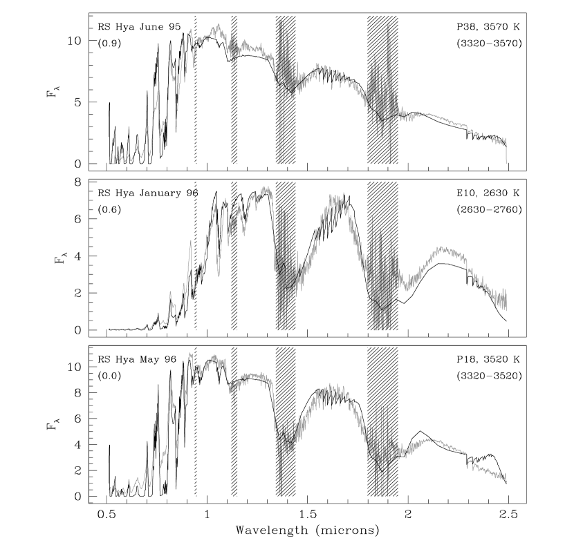
Figure 3: This figure shows the empirical spectrum (grey) and one of the best fitting models (black) for RS Hya as observed in June 1995 (upper panel), January 1996 (middle panel) and May 1996 (lower panel). The flux densities per unit wavelength are in arbitrary units. The estimated phase of observation is given on the left side of each plot. On the right side, the plotted model is identified (see Table 2). The range of temperatures ($T_{1.04}$) reached by models that provide fits of similar quality is indicated underneath. Shaded strips are the regions of strong telluric absorption which are excluded during comparison.

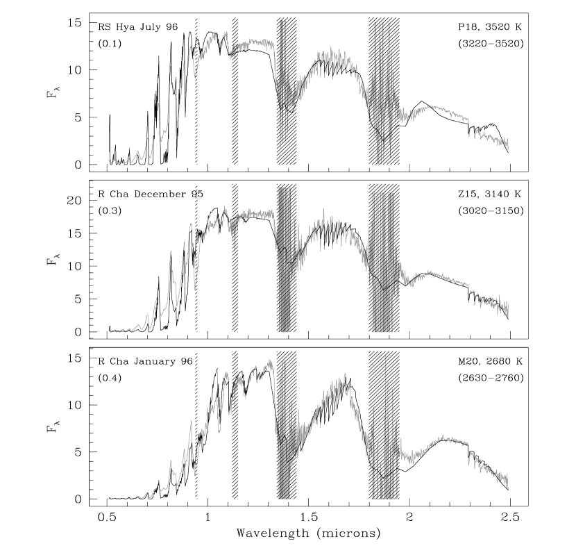
Figure 4: Same as Fig. 3 but for RS Hya in July 1996 (upper panel), and for R Cha in December 1995 (middle panel) and January 1996 (lower panel).

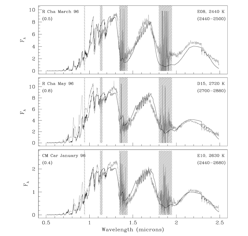
Figure 5: Same as Fig. 3 but for R Cha in March 1996 (upper panel) and May 1996 (middle panel), and for CM Car in January 1996 (lower panel). Note that for the March 96 spectrum of R Cha the $T_{\rm eff}$ values of the ‘best fit’ models reach as low as 2160 K ($T_{\rm 1.04}$ values are given in the figures).

For a first, automatic selection of appropriate models, we compare each observed spectrum with the entire set of model spectra and quantify the quality of each fit with a $\chi^{2}$ value. In computing $\chi^{2}$, care is taken to exclude portions of the spectra which are strongly affected by telluric absorption (see Fig. 2). Otherwise, equal weight is given to each data pixel (i.e. 950 points below 1 $\mu$m and 2400 points above). Rather than rejecting all models but the one with the minimum $\chi^{2}$, we keep the 5 to 10 models with $\chi^{2}$ values not significantly larger than the minimum value. This is justified as follows. Mathematically speaking none of the resulting $\chi^{2}$ values is good : the difference between the data and the best fitting models cannot be explained by observational errors alone. In that situation, the search for best fits still makes sense, but the definition of the rejection criterion becomes more arbitrary. Different ‘best’ solutions can be obtained by giving different features (band strengths, band shapes, continuum colours, etc.) different relative weights in the $\chi^{2}$. Our threshold on the naturally-weighted $\chi^{2}$ value was set so that the selected models approximatively cover the range one would obtain by modifying weights in various reasonable ways.

Eye inspection followed the automated pre-selection, taking into account the following arguments. The model reproduction of the spectral features are considerably better in the near-IR as compared to the region below 1 $\mu$m. There are various conceivable model inadequacies in the optical domain responsible for this disparity. First, the simple treatment of TiO bands dominating the optical spectrum may result in appreciable inaccuracies of band depths, in particular for very strong features (Section 2.1; cf. BSW96). Second, the pronounced temperature contrast between continuum-forming layers and the upper layers where the molecular bands are formed makes the shapes and depth of these TiO bands strongly dependent on the subtle details of the outer atmospheric stratification in the Wien part of the spectrum. Third, if dust particles were formed in the outer atmosphere, this would strongly affect the optical spectral region (Bedding et al. 2001; cf. Section 4.2). As a consequence of the above, low weight is given to the quality of fits to the individual spectral features in the optical part of the spectrum. However, it should be noted that the overall energy distribution in the region below 1 $\mu$m and the ratio of optical to near-IR light do play a significant role in constraining the model fits.

As the result of the above selection, we are left for each observed spectrum with a few model spectra that qualify as satisfactory : the energy distribution, the relative band strengths and shapes are reproduced to a level that was unexpected considering the complexity of these objects and the limited range of explored model parameters. Because of the degeneracies in the models mentioned previously, the qualifying models span a wide range of parameters. Even the effective temperature shows significant dispersion among acceptable solutions.

In Fig. 3, 4 and 5 we show comparisons with typical ‘best fitting’ model spectra. For RS Hya, the four spectra shown are reproduced reasonably well by the models. The best fitting models for the January 1996 spectrum deviate beyond 2 $\mu$m. These deviations in the energy distribution are consistent with the estimated observational uncertainties at the $2\sigma$ level only. In the case of R Cha, the agreement between the models and the observed spectra is very good for the December 1995, January 1996 and May 1996 spectra. The March 1996 spectrum of this star stands out with a particularly red slope around 1 – 1.3 $\mu$m and a corresponding excess beyond 2 $\mu$m, a behaviour that resembles the January 1996 spectrum of RS Hya. It is also striking that these two spectra have particularly red slopes between 1 and 1.3 $\mu$m. We discuss them in detail in Sect. 4.2. For CM Car, the best fits are also satisfactory.

We re-evaluated the visual phases of the observed stars based on the appearance of the available time series of observed spectra. A phase diagnostic feature is the Paschen $\beta$ line which appears in emission near maximum (Fox et al. 1984). The re-estimated phases are uncertain to $\pm$0.1 cycles. For the CM Car spectrum the uncertainties could be larger as there is no time series available. For the models, the visual phase was estimated from the bolometric light curves by BSW96 and HSW98, assuming an offset of about 0.1 cycles between the two (Lockwood & Wing 1971). Uncertainties of this offset estimate, irregular shapes of luminosity curves (see Figs. 1 to 3 of BSW96 and HSW98), and deviations of up to several days between the formal pulsation period of the parent star and actual mean periods of pulsation series, may readily result in phase uncertainties of the order of 0.1 to 0.2.

The phase matching between the observed spectra and the best-fitting model spectra shows random discrepancies. For most cases, the agreement between the observed phase and the phase of the best-fitting model spectra is within 0.3 cycles. This is consistent with the two quoted uncertainties. There are exceptions however (e.g. the December 1995 spectrum of R Cha), where the set of good model fits covers a wide range of phases. This is not surprising in view of the degeneracies illustrated in Fig. 2.

We carried out this model fitting procedure for the other Miras in the sample, which have different periods, and found similar levels of agreement for more than 80 % of the observed spectra. In summary, the overall shape and the gross features of the observed spectra are well reproduced by the models. Most broad band energy distributions can be adjusted to within the observational uncertainties, despite the limited parameter and phase or cycle coverage of the available models (see also Sect. 4.1). The shapes of wide molecular bands can be adjusted very well when the comparison is restricted to a subsection of the spectrum. The constraint set by the complete energy distribution is heavy, and resulting imperfections of the best fits must be blamed at least partly on the small size of the model set.

Considering the models and data as samples and looking at specific spectral features will throw more light on the systematics in the respective behaviours of the models and the observations. This is the aim of the following section.

4 Behaviour of specific spectral features

It is beyond the scope of this paper to study the numerous features of Mira spectra individually. We have chosen to focus on three specific features: (1) the broad band colours, because they are the most commonly measured quantities; (2) the spectral region between 1 and 1.3 $\mu$m, which apart from displaying various slopes both for the models and the observed spectra is currently considered to contain near-continuum wavelength regions; (3) a few near-IR molecular bands for which specific narrow band filters exist, thus making them more accessible to observations. Among the latter, H₂O is given most attention because of its potential relevance to the interpretation of the near-IR angular diameter measurements (TLS03).

4.1 The broad-band colours

For cool stars the observed broad-band colours and magnitudes are often used for estimating luminosities and effective temperatures. In this section, we investigate the trends seen in the observed and model predicted colours. Fig. 6 shows a set of broad-band colours derived from the model and the observed spectra. No extinction correction is applied to the colours on this figure. The arrows indicate the effect of interstellar extinction for A_V=1 (greater than the values derived for the three stars of Figs. 3, 4 and 5). Also shown are the 2$\sigma$ uncertainties of the observed colours. Given the scatter, the interstellar extinction would not appreciably affect the trends seen. Within these uncertainties, the plots show considerable overlap between the loci of the observed and the model predicted colours. Systematic offsets between the colours predicted by the models and those observed, if any, are small.

Despite the limited range of explored model parameters and the uncertainties involved in modeling the Wien part of the spectrum, the extent of observed broad-band colour distributions is reproduced rather well. The largest difference is seen in $J-K$ and $H-K$, where the observations reach redder colours than the models. The selection of spectra with $J-K>1.45$ leads to a homogeneous subsample of spectra similar to the March 1996 observation of R Cha and the January 1996 observation of RS Hya, two spectra already pointed out in Sect. 3. These two spectra show a red slope in the 1 $\mu$m region and also display IR excess beyond 2 $\mu$m when compared with dust-free model spectra. Anticipating the discussion of Sect. 4.2, we note that this hints at the presence of reddening, possibly due to the presence of atmospheric and circumstellar dust, or at the existence of additional sources of atmospheric opacity that may be currently missed or underestimated in the models.

Figure 6: Broad-band colours for the observed spectra (solid circles) and the model spectra (open circles). Also shown are the 2$\sigma$ uncertainties of the observed colours and the Milky Way extinction vector for A_V=1.

4.2 The spectral slope between 1 and 1.3 $\mu$m

A close study of the nature of the model and observed spectra reveals distinct differences in the slope of the 1 $\mu$m region. The models conspicuously display rather flat spectra in this region compared to the variety of slopes found in the data. The spectral window around 1.04 $\mu$m is a particularly important part of the spectrum of Mira-type stars, as it is often considered one of the best access points to the near-IR continuum (Jacob & Scholz 2002). The nature and possible origin of this disparity in slope is the focus of this section.

Blue slopes in the region between 1 and 1.3 $\mu$m were commented upon by LW2000. While studying phase offsets between the cycles followed by the strength of VO (1.05 $\mu$m) and other spectral signatures (cf. Alvarez & Plez 1998), they noted that the blue slopes tend to occur just before the disappearance (or strong reduction) of VO and other molecular bands. Although their argument was based on a small number of stars for which phase coverage was sufficient, they suggested that this happens just before, or in any case close to maximum light (spectra that still display Paschen lines but show no remaining VO absorption occur slightly later in the same pulsation cycle).

The new phase 0.8 models computed for the P series indeed display blue slopes in the 1 $\mu$m region, while still displaying deep molecular bands characteristic of low temperatures (see Appendix A). As shown in Sect. 3, a significant number of observed spectra can only be adjusted with models having these properties (Figs. 3, 4 and 5). The 0.8 models of the Z series also display blue $1-1.3\,\mu$m slopes but this is less surprising as it agrees with an otherwise warm energy distribution. In the models, these blue $1-1.3\,\mu$m slopes appear only shortly before maximum light when the newly emerging shock front is still in deep layers and one can probe the deep hot layers. This result clarifies the empirical trend found by LW2000.

The global behaviour of the slope in the $1-1.3\,\mu$m region is illustrated in the narrow-band [1.0425] – [1.305] versus [1.305] – [2.25] colour-colour plot shown in the lower panel of Fig. 7. The colours are measured through square filters centered at 1.0425, 1.305 and 2.25 $\mu$m, with respective full widths of 5, 20 and 20 nm ; they are given in magnitudes and take the value 0 for Vega.

The dynamical models (open circles) occupy a very narrow range of values in [1.0425] – [1.305] compared to the observed data (crosses). The dynamical ranges of the [1.305] – [2.25] colours are reasonably consistent for the model and observed spectra. The observed spectra that show the bluest [1.0425] – [1.305] colours in the plot (i.e. bluest slope in the 1 – 1.3 $\mu$m region), also display Paschen line emission and deep molecular bands. Spectra with warm energy distribution and shallow molecular bands have small values in both the pseudo-continuum colours and hence occupy the lower left quadrant of the plot.

The lower panel of Fig. 7 also shows that several observed spectra have very red slopes in the $1-1.3\,\mu$m region, while there are no models with [1.0425] – [1.305] greater than 0.9. The observed spectra with such red slopes include and resemble the January 1996 spectrum of RS Hya and March 1996 spectrum of R Cha (cf. Sect. 3). The upper panel of Fig. 7 gives a comparative view of the multi-epoch spectra of these two selected Miras and the model spectra. From this plot it is clear that the variation of the colour [1.0425] – [1.305], which is indicative of the 1 $\mu$m slope, with phase is not only larger for the observed Miras as compared to the dynamical models, but also the variation is along a different direction.

Figure 7: Lower panel: Model predicted (open circles) and observed (crosses) narrow-band colours. [1.0425] – [1.305] measures the slope in the $1-1.3\,\mu$m region, [1.305] – [2.25] is a narrow-band analog of J-K. Upper panel: Here, the models (open circles) and two individual Miras RS Hya (solid triangles) and R Cha (solid squares) are plotted. The numbers at the top indicate the phase of observation of the RS Hya spectra; (1:2:3:4:5 correspond to 0.8:0.9:0.0:0.1:0.6) and the numbers on the lower side are for R Cha; (1:2:3:4 correspond to 0.8:0.3:0.4:0.5).

Figure 8: Location of the dusty models (solid circles) in the two-colour plot of Fig. 7. Open circles are dust-free models and crosses are observations. The arrow corresponds to $A_{v}=1$ with the Milky Way interstellar extinction law.

Opacity data in the 1 $\mu$m region might be the most likely origin for the lack of red model slopes. The current models may overlook or underestimate sources of opacity. Independent evidence in favour of additional opacities at large radii comes from wavelength and phase-dependent angular diameter measurements (e.g. Young et al. 2000 for $\chi$ Cygni). The sources of such opacities could be molecules or dust-grains which would significantly affect both the spectra and the disk brightness distribution.

The molecular sources of opacities of the models were assembled according to their importance in normal red giants, and may indeed be incomplete at low temperatures reached in outer Mira atmospheres. Relevant molecular absorption sources that are already included, but for which the adopted opacities may be incomplete, are TiO, VO and H₂O. The choice of one or the other particular combination of the various published opacity tables for these three molecules plays a decisive role in cool dwarf star models (P. Hauschildt, private communication). One may also extend the list of potential molecular opacity sources to more exotic species such as YO, ZrO or ScO, that reach observable proportions in S star models (e.g. Piccirillo 1980), or to molecules observed in dwarfs or subdwarfs (CN, HCN, CaH, FeH to cite a few; see e.g. Allard & Hauschildt, 1995, for a more extended list). We have not explored these possibilities, hence it is beyond the scope of this paper to give a quantitative discussion on the molecular opacity issue and this point is left open to future studies.

The formation of dust in the outer atmospheres of at least some Miras, on the other hand, may be considered a fact supported by the evolutionary transition from Miras to dust-enshrouded OH/IR sources. Ferguson et al. (2001) give reasons for dust formation and absorption around cool static red giants. Observationally, some interferometric and spectroscopic measurements indicate that inner edges of dust shells might be as close 2 or 3 continuum radii from the star’s centre (e.g. Danchi et al. 1994; Danchi & Bester 1995; Lobel et al. 2000; Lorenz-Martins & Pompeia 2000). Bedding et al. (2001) have studied the occurrence of dust in the atmospheres of Miras and its effect on their spectra. Dust thermodynamically fully coupled to the surrounding gas is shown to affect the 1.04 $\mu$m passband and to distort the brightness distribution considerably. This prompted us to investigate the role of dust in the 1 $\mu$m region. In Fig. 8, we show the loci of the dusty models from Bedding et al. (2001) in the same two colour diagram as in Fig. 7. The blue end of the dusty models overlaps with the dust-free models. The dusty models do show redder slopes and display large [1.0425] – [1.305] values but they also have a strong excess in the [1.305] – [2.25] colour. Nevertheless, we compared the spectra of the three Miras presented in Figs. 3, 4 and 5 with the dusty models. Only for two spectra, namely the March 1996 spectrum of R Cha and January 1996 spectrum of RS Hya better agreement is obtained with the dusty models. These are the spectra already identified as particularly red in Sect. 3, and they are also representative of all the spectra with particularly large values of $J-K$ and $H-K$ in Fig. 6. The two new ‘best fits’ are shown in Fig. 9.

In view of the above comparison of observed spectra with the dusty models, a few important points are worth mentioning. Firstly, Bedding et al. (2001) is an exploratory study on the occurrence of dust only in a small subset of the available models, and they have tested only a few values of the dust condensation fraction. Therefore remaining imperfections in the fits of the energy distributions of the two stars of Fig. 9 are not surprising. The changes induced by the presence of atmospheric dust go in the right direction. Bedding et al. (2001) have also adopted a particular dust composition ; other assumptions would lead to somewhat different effects on the colours (the arrow in Fig. 8 shows the effect of average Milky Way interstellar dust). Secondly, the fact that for most of the observed spectra the fit quality is not improved with the few available dusty models does not by itself exclude the presence of some atmospheric or circumstellar dust.

There is some indication of variation of dust with phase but it is difficult to make any quantitative statement regarding this in the absence of proper phase coverage of the dusty models. This can be better appreciated by looking at the loci of the two individual stars in Fig. 7. For R Cha and RS Hya the dusty models fit better to phases 0.5 ($\pm$0.1) and 0.6 ($\pm$0.1) respectively. For R Cha the rest of the observed spectra (phases 0.3, 0.4 and 0.8) have similar level of fits with dusty and dust-free models. For RS Hya dusty models do not provide good fits to the rest of the observed spectra (phases 0.8, 0.1, 0.9 and 0.0). This is consistent with a general scenario in which dust effects are maximum at minimum light and hence at the lowest temperatures.

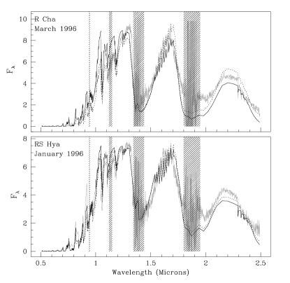
Figure 9: This figure shows the March 96 spectrum (grey) of R Cha (upper panel) and the January 96 spectrum (grey) of RS Hya (lower panel). Also plotted are the best fitted dust-free (solid) and dusty (dotted) models. Fluxes are given in arbitrary units of energy per unit wavelength.

To conclude the above discussion, we consider it likely that the disparity seen in the slope around 1 $\mu$m between the models and the observed spectra is partly due to dust.

4.3 The molecular bands

The spectrophotometric features due to H₂O and VO are amongst the most prominent molecular bands seen in the spectra of Miras. In this section, we compare these bands in the observed and the model spectra. For band measurements, we use narrow-band filters similar to those of Wing (1967) and White & Wing (1978), adopting the passbands defined by Bessell et al. (1989; see Fig. 3 of Alvarez et al. 2000). The indices are the ratios between the fluxes measured through a passband in the molecular band and a passband that is not or little affected; like colours, they are expressed in magnitudes and take the value 0 for Vega. The VO band at 1.05 $\mu$m is measured by the [105] – [104] colour index. For H₂O, we consider the index [220] – [200] located in the wings of the 1.9  $\mu$m band. In Fig. 10, we plot the two molecular indices as a function of two broad-band colours.

Figure 10: H₂O and the VO indices as a function of the $R-I$ and $V-K$ broad-band colours for the model (open circles) and the observed (crosses) spectra. The data points for RS Hya and R Cha are highlighted, respectively, as solid triangles and squares. Overplotted are the static giant models XX (metallicity +0.5: dotted line) and YY (metallicity -1.0: solid line).

The values of the VO index span similar ranges for the models and the observations, which is satisfactory. A small but significant offset in colour between models and data is present as one moves to the red ends of the distributions. The value of this offset is larger in the plot of VO vs. $V-K$, as expected from the relation between $V-K$ and $R-I$ (which agrees well between model and data for the large values of $V-K$ that are relevant here). At a given colour, observed VO bands appear stronger than the model predicted ones. The Wing VO index considered above measures the molecular absorption at 1.054 $\mu$m, i.e. somewhat off the band’s deepest point (near 1.06 $\mu$m in the models). If we use a modified index with a more centrally located passband, we find that the VO values for the models increase by about 0.1 magnitudes in the VO vs. colour plots, while the values for the empirical spectra remain essentially unchanged. The offset is slightly reduced. The fact that data and models have different sensitivity to a change in the adopted index is due to the shape of the modeled absorption bands, which do not precisely agree with the observed shapes. Here, the opacity data (and possibly the overlap with bands from various molecules) are the most likely origin of the discrepancies.

For the H₂O index we note that the overlap between the observed and the model points is less satisfactory. The plot shows that for blue $R-I$ and $V-K$ colours the observed spectra display stronger H₂O bands compared to the model predicted values (see Matsuura et al. 1999 for additional observations of early M type stars with significant water bands). On the other hand the models show strong H₂O bands ($>$ 1.3) towards the red end and no observations are found in that region of the diagrams. The models with these strong H₂O bands are the near-minimum P and M models and all the O models. The range of model-predicted H₂O indices is much larger than the variation seen with phase for individual observed Miras.

Random selection of an observed spectrum and a model spectrum with similar H₂O index, shows good agreement in the shape and strength of the H₂O bands at 1.4 $\mu$m and 1.9 $\mu$m. Different indices, designed to measure absorption in the shorter wavelength wing of the 1.9 $\mu$m band and the wing of the 1.4 $\mu$m band, show similar trends in the H₂O vs. colour plots. These two arguments indicate that the disparity seen in the plots is not due to the choice of one particular index.

The other parameters in the plots of Fig. 10 are the broad-band colours. Fig. 6 doesn’t reveal any obvious problem with the colours. The uncertainty estimates on the observed broad band colours by LW2000 have been checked and found correct. However, in addition to these random errors there might be systematic errors in the merging procedure between optical and near-IR data, in particular for spectra with very steep energy distributions near 1 $\mu$m (see models of Fig. 1 or 2). This might have led to systematically bluer $V-K$ values for these particular spectra. Going back to the original data, we estimate that 0.5 mag is an upper limit of such errors, if present (such an effect is not incompatible with Fig. 6). For stars without such dramatic features around 1 $\mu$m, we find no reason for systematic errors. The merging procedure would not affect the $R-I$ colour. We therefore conclude that observational uncertainties in the broad band colours might contribute but cannot by themselves explain the offsets in the index-colour plots.

Metallicity could be one of the reasons for the disparity in the plot of H₂O vs. $V-K$. The pulsating star models are computed only for solar metallicity. To show the likely effect of metallicity, we have plotted lines showing static giant models with two extreme metallicites (Z/Z_⊙=+0.5 and -1.0) but identical masses and luminosities (1 M_⊙, $10^{4}$ L_⊙; Bessell et al. 1989, 1991; see Bessell et al. 1991 for loci of evolutionary tracks). The lower metallicity models have warmer colour temperatures. In the dynamical case, it is likely that lower metallicity also shifts the locus of the dynamical spectra to bluer colours, while pulsation might still allow for strong H₂O bands. A negative correlation between the H₂O bands and metal lines in the $K$ band has been suggested by LW2000: they noted that among empirical spectra with similarly warm energy distributions those with the strongest H₂O bands tend to have the weakest absorption features of CO and metals (Na, Ca). All the spectra with an H₂O index above 0.6 and $R-I<2.5$ belong to stars labelled as potentially metal poor by LW2000. The construction of pulsating models at subsolar metallicity and its effect on spectral features (Lançon, Scholz & Wood, in preparation) would help resolve this issue, and we may expect that intrinsically warmer models with large pulsation amplitudes will explain some of the relatively blue spectra with deep H₂O absorption.

But metallicity alone cannot account for the discrepancies in Fig. 10. This is made clear by the locus of the two individual Miras R Cha and RS Hya. For these two stars the loci of the observed points follow a line that crosses the locus of the solar metallicity dynamical models. In the H₂O vs. $R-I$ plot, the effect of metallicity is not that pronounced as compared to the $V-K$ colour. Where else could the origin of the discrepancy lie? The water bands depend on the density and temperature stratifications, but probably also on the treatment of shocks and on molecular relaxation times, etc. Apart from metallicity, mild increases of C/O ratios within the tolerance of M type classification may play some role. Potential answers are as numerous as the model ingredients and only speculations can be made at this stage. Future modeling will show whether some physical assumption must be modified or whether a more complete exploration of the model parameters is sufficient.

5 Discussion and Conclusion

In this paper we have compared the model predicted spectra of BSW96 and HSW98 with observations of Miras covering the wavelengths from 0.5 to 2.5 $\mu$m. For the three Miras with periods similar to those of the models, namely RS Hya, R Cha and CM Car, the energy distributions over the entire spectral range are reproduced reasonably well, considering (i) the observational uncertainties and (ii) the large number of relevant model parameters and the limited number of models actually available. In many cases, the overall shape is modeled similarly well for stars with different periods. General agreement is also found between the loci of the empirical and synthetic data points in plots combining two standard broad band colours. This may indicate that period is not the most important parameter in determining the range of resulting spectrophotometric properties.

When investigating specific spectral features, it is not possible to fully assess which discrepancies between models and observations are simply the consequence of the limited sample of available synthetic spectra. Discrepancies are seen in the slope of the spectra between 1 and 1.3 $\mu$m. Most models display a flat continuum whereas the observed spectra show both blue and red slopes in this wavelength region. Models close to maximum (phase 0.8) do account for the blue slopes. New 0.8 phase models of the P series were essential to fit to a number of the observed spectra. In a few cases, models with dust produce red slopes in this 1 $\mu$m region and fit better to the observed spectra. However, not all the spectra having red slopes are well represented by the limited available dusty models. It is also worth noting that, when dust helps achieving good agreement for one spectrum of a star, dust-free models provide satisfactory fits at other phases of the same star. This may indicate a phase dependence of dust formation. But a detailed phase-correlated study, involving exhaustive dust modeling, needs to be done before arriving at any definitive conclusion. Missing molecular opacities in the 1 $\mu$m region might also be a cause for disparities at those wavelengths.

The agreement between observed and model-predicted molecular bands is far from perfect. For VO (1.05 $\mu$m), the range of predicted index values is consistent with observations, but it is seen that for red $V-K$ or $R-I$ colours the models produce weaker VO indices than are observed. For H₂O, the models predict very strong absorption bands for the reddest spectra. None of the observations of LW2000 reach these extreme values of the H₂O absorption index. At the blue end of the colour distribution, on the contrary, the observed H₂O bands are stronger than the model-predicted ones. On one hand, problems of completeness and of approximations of opacities used in the models (BSW96, HSW98 and Brett 1990) may be significant. These are essentially mean opacities rather than extinction coefficients based on an opacity distribution function or an opacity sampling technique, neither of which can be applied directly to a dynamic atmosphere with pronounced velocity stratification (cf. Scholz 2003; for recent approaches to opacity distribution functions see Baschek et al. 2001, Wehrse 2002). For H₂O absorption, the empirical data of Ludwig (1971) were adopted. On the other hand, features such as the H₂O band depths and shapes are sensitive to the precise structure of the outer layers of the atmospheres, which might have to be further improved. In some of the studied models (in particular P18, P38, see the Appendix), the shape of the bands clearly shows the combination of emission and absorption components. Such a phenomenon was noted in observations at longer wavelengths (Yamamura et al. 1999), but is not obvious in the near-IR spectra of LW2000. Because the H₂O bands carry the potential of revealing the extended atmospheric structure and, thus, improving the interpretation of stellar diameter measurements (TLS03), it will be important to continue to invest effort into their precise modeling.

Finally, our study underlines the importance of using data with a broad wavelength coverage when testing the validity of the models. Any restriction of the observed range makes fits easier to achieve and thus less constraining. Currently, the determination of fundamental stellar parameters from spectral fits remains difficult even when optical and near-IR spectra are available simultaneously. Fits result in a rather wide collection of equally acceptable sets of fundamental stellar parameters. One reason for this is that the most common parameters, effective temperature, mass, luminosity, metallicity are not sufficient to describe the structure of a Mira atmosphere ; hidden parameters that provide a more precise description may have effects that compensate each other partly, leading to degeneracies. Other reasons are to be found in the ‘primitive’ nature of the models and the restricted phase-cycle-parameter coverage. Indeed, it is the quality of the ‘best fits’ between the available models and observations that in the end also defines how tightly the model rejection criteria can be set. Improved parameter coverage and model input physics should lead to better fits to the spectral data, and thus enable us to discriminate between model parameters more radically. Along with this, increased wavelength coverage in the data and enhanced spectral resolution of certain features would help in constraining the parameter estimates. As an example, one might investigate the relative strengths of OH and CO lines in the 1.5 – 1.7$\,\mu$m window, which differ significantly from one Mira to the other (LW2000). High-accuracy, multibaseline, near-continuum interferometric observations covering a large range of phase-cycle will help in retrieving the monochromatic disk brightness distribution which gives the only direct information regarding the geometry and physics of a Mira and constrain the stellar parameters by defining the proper atmospheric stratification. Achieving this and improving the situation will also be a task of future observational and theoretical work.

Appendix A Parameters for the time series of the models.

In Table 2, we list the parameters of the time series of the Mira models. This is an extract of Table 3 of BSW96 (Z, D, E series) and Table 2 of HSW98 (P, M, O series). Newly included are the phase 0.2 and 0.8 models of the P and the M series.

Table 2: Parameters of the time series of the new Mira models. The columns: visual phase $\phi_{vis}$; luminosity $L$; Rosseland radius $R$; 1.04 near-continuum radius $R_{1.04}$; effective temperatures $T_{\rm eff}$ and $T_{1.04}$). The model names consist of a letter defining the series followed by the pulsation phase $\times$ 10.

Mod.	$\phi_{vis}$	$L$	$R$	$R_{1.04}$	$T_{\rm eff}$	$T_{1.04}$
		($L_{\odot}$)	($R_{\rm p}$)	($R_{\rm p}$)	(K)	(K)
Z08	0+0.8	8140	0.90	0.90	3770	3760
Z10	1+0.0	7650	1.10	1.11	3350	3340
Z12	1+0.24	6860	1.13	1.13	3220	3220
Z15	1+0.5	3860	0.89	0.89	3150	3140
Z18	1+0.8	8230	0.90	0.90	3770	3770
Z20	2+0.0	7750	1.11	1.12	3350	3340
Z22	2+0.24	6840	1.13	1.13	3220	3210
Z25	2+0.5	3830	0.89	0.89	3140	3140
D08	0+0.8	3500	0.90	0.90	3050	3050
D10	1+0.0	4490	1.04	1.04	3020	3020
D12	1+0.2	4920	1.09	1.10	3010	3010
D15	1+0.5	2210	0.91	0.90	2710	2720
D18	1+0.8	3510	0.90	0.90	3050	3050
D20	2+0.0	4560	1.04	1.05	3030	3020
D22	2+0.2	4760	1.09	1.09	3000	2990
D25	2+0.5	2170	0.91	0.90	2690	2700
E08	0+0.83	4790	1.16	1.07	2330	2440
E10	1+0.0	6750	1.09	1.09	2620	2630
E11	1+0.1	8780	1.12	1.11	2760	2770
E12	1+0.21	7650	1.17	1.15	2610	2640
P05	0+0.5	1650	1.20	0.90	2160	2500
P08	0+0.8	4260	0.74	0.74	3500	3500
P10	1+0.0	5300	1.03	1.04	3130	3120
P12	1+0.23	4540	1.38	1.30	2610	2680
P15	1+0.5	1600	1.49	0.85	1930	2560
P18	1+0.8	4770	0.77	0.77	3520	3520
P20	2+0.0	4960	1.04	1.04	3060	3060
P22	2+0.18	4400	1.32	1.26	2640	2700
P25	2+0.5	1680	1.17	0.91	2200	2500
P28	2+0.8	5200	0.79	0.79	3550	3550
P30	3+0.0	5840	1.13	1.14	3060	3050
P35	3+0.5	1760	1.13	0.81	2270	2680
P38	3+0.8	5100	0.78	0.78	3570	3570
P40	4+0.0	4820	1.17	1.16	2870	2880
M05	0+0.5	1470	0.93	0.84	2310	2420
M08	0+0.75	4780	0.81	0.81	3320	3320
M10	1+0.0	4910	1.19	1.18	2750	2760
M12	1+0.26	2990	1.33	1.12	2300	2500
M15	1+0.5	1720	0.88	0.83	2460	2530
M18	1+0.75	4840	0.81	0.81	3310	3310
M20	2+0.0	4550	1.23	1.20	2650	2680
M22	2+0.27	2850	1.27	1.10	2330	2490
O05	0+0.5	5020	1.12	1.00	2050	2130
O08	0+0.8	4180	0.93	0.91	2150	2170
O10	1+0.0	7070	1.05	1.01	2310	2360

The P and M models at phase 0.8 are particularly warm and compact, a phenomenon already found in the Z and D fundamental-mode pulsation series. As the new shock front emerges from deep layers, densities are fairly low in the outer and middle parts of the atmosphere and unity continuous optical depth is reached at small distances from the star’s centre. The star appears small in continuum bandpasses and effective temperatures are high. The effect is particularly impressive for the self-excited HSW98 model series for which differences between pre-maximum and maximum continuum radii are of the order of 0.3 parent star radii, resulting in dramatically higher $T_{\rm 1.04}$ effective temperatures around phase 0.8 than at maximum despite similar luminosities. The spectra have relatively blue colours (bluer than at phase 0.0 or 0.5), but significant molecular features nevertheless. The blue slope between 1 and 1.3 $\mu$m is particularly impressive for models P18 and P38. The remarkably irregular light curve of the P model series (see HSW98) shows that in these two cycles maximum light was actually reached before the phase labelled 0 (see Sect. 3 for uncertainties of phase adjustments).

Figure 11: Molecular emission and absorption in models from the P series. The top panel shows 4 models, normalized at 2.2 $\mu$m to highlight differing shapes in that region. P15 - solid; P18 - dotted; P20 - short dash; P38 - dot-short dash. The two lower panels compare the model spectra of P15 (middle) and P18 (bottom) with the pure continuum spectrum (short dash) and spectrum without H₂O absorption (dotted) without any normalization. The continuum spectrum is obtained by setting all molecular opacities to zero after the model atmosphere has been constructed with the complete opacity list, and for the spectrum without H₂O only the opacities due to H₂O are switched off.

Models P18 and P38 also stand out because of the “peculiar” shape of their water bands. In the wings of what usually appears as a broad absorption band, i.e. around 2.05 and 2.4 $\mu$m, bumps that could be described as “emission shoulders” are present (top of Fig. 11). In the H window, these “shoulders” are not as obvious but manifest only as a modification of the curvature of the resulting energy distribution. This phenomenon has never been mentioned in work based on spectroscopy below 2.5 $\mu$m but has been suggested to occur at longer wavelengths (Yamamura et al. 1999, Matsuura et al. 2002). The middle panel of Fig. 11 shows that excess emission above the pure continuum level can sometimes occur in the K band in a way that would be extremely difficult to identify in low resolution spectra.