A New Non-Parametric Approach to Galaxy Morphological Classification

Abstract

We present two new non-parametric methods for quantifying galaxy morphology: the relative distribution of the galaxy pixel flux values (the Gini coefficient or $G$) and the second-order moment of the brightest 20% of the galaxy’s flux ($M_{20}$). We test the robustness of $G$ and $M_{20}$ to decreasing signal-to-noise and spatial resolution, and find that both measures are reliable to within 10% for images with average signal-to-noise per pixel greater than 2 and resolutions better than 1000 pc and 500 pc, respectively. We have measured $G$ and $M_{20}$, as well as concentration ($C$), asymmetry ($A$), and clumpiness ($S$) in the rest-frame near-ultraviolet/optical wavelengths for 148 bright local “normal” Hubble type galaxies (E-Sd) galaxies, 22 dwarf irregulars, and 73 $0.05<z<0.25$ ultra-luminous infrared galaxies (ULIRGs). We find that most local galaxies follow a tight sequence in $G-M_{20}-C$, where early-types have high $G$ and $C$ and low $M_{20}$ and late-type spirals have lower $G$ and $C$ and higher $M_{20}$. The majority of ULIRGs lie above the normal galaxy $G-M_{20}$ sequence, due to their high $G$ and $M_{20}$ values. Their high Gini coefficients arise from very bright nuclei, while the high second-order moments are produced by multiple nuclei and bright tidal tails. All of these features are signatures of recent and on-going mergers and interactions. We also find that in combination with $A$ and $S$, $G$ is more effective than $C$ at distinguishing ULIRGs from the “normal” Hubble-types. Finally, we measure the morphologies of 49 $1.7<z<3.8$ galaxies from HST NICMOS observations of the Hubble Deep Field North. We find that many of the $z\sim 2$ galaxies possess $G$ and $A$ higher than expected from degraded images of local elliptical and spiral galaxies, and have morphologies more like low-redshift ULIRGs.

1 INTRODUCTION

The evolution of the physical structure of galaxies is one of the keys to understanding how matter in the universe assembled into the structures we see today. The most accessible tracer of a galaxy’s physical structure is its morphology, i.e. the organization of its light (stars and dust), as projected into our line of sight and observed at a particular wavelength. As we examine more distant galaxies, we find that galaxy morphologies become increasingly chaotic. The disk and spheroidal structures abundant in the local universe disappear at early times in the universe (e.g. Abraham et al. 1996, Abraham & van den Bergh 2002). The emergence of the local Hubble sequence of spiral and elliptical galaxies at late times is one of the predictions of the hierarchical picture of galaxy assembly.

While the first morphological studies sought to describe the variety of galaxy shapes and forms, the goal of present-day morphological studies is to tie the spatial distribution of stars to the formation history of the galaxy. A major obstacle to this goal has been the difficulty in quantifying morphology with a few simple, reliable measurements. One tack is to describe a galaxy parametrically, by modeling the distribution of light as projected into the plane of the sky with a prescribed analytic function. For example, bulge-to-disk light ratios may be computed by fitting the galaxy with a two-component profile, where the fluxes, sizes, concentrations, and orientations of the bulge and disk components are free parameters (Peng et al. 2002, Simard et al. 2002). This B/D ratio correlates with qualitative Hubble type classifications, although with significant scatter. Unfortunately, there is often a fair amount of degeneracy in the best-fitting models and B/D ratios, and structures such as compact nuclei, bars, and spiral arms introduce additional difficulty in fitting the bulge and disk components (e.g. Balcells et al 2003). A related approach is to fit a single Sersic profile to the entire galaxy (Blanton et al. 2003a). Profiles with high Sersic indices are interpreted as bulge-dominated systems, while low Sersic indices indicate disk-dominated systems. However, not all bulges have high Sersic index values - some are exponential in nature (Carollo 1999), so not all objects with bulges will produce intermediate or high Sersic indices. Both the one-component and multiple-component fitting methods assume that the galaxy is well described by a smooth, symmetric profile - an assumption that breaks down for irregular, tidally disturbed, and merging galaxies.

Non-parametric measures of galaxy morphology do not assume a particular analytic function for the galaxy’s light distribution, and therefore may be applied to irregulars as well as standard Hubble type galaxies. Abraham et al. (1994, 1996) introduced the concentration index $C$ (which roughly correlates with a galaxy’s B/D ratio) and Schade et al. (1995) put forward rotational asymmetry $A$ as a way to automatically distinguish early Hubble types (E/S0/Sa) from later Hubble types (Sb/Sc) and classify irregular and merging galaxies. Subsequent authors modified the original definitions to make $C$ and $A$ more robust to surface-brightness selection and centering errors (Wu 1999, Bershady et al. 2000, Conselice et al. 2000). The third quantity in the “$CAS$” morphological classification system is a measure of a galaxy’s residual clumpiness $S$, which is correlated with a galaxy’s color and star-formation rate (Isserstedt & Schindler 1986; Takamiya 1999; Conselice 2003). Other more computer-intensive approaches to galaxy classification such as artificial neural networks and shapelet decomposition have also been applied to local and distant galaxies. Artificial neural networks are trained by an astronomer on a set of galaxies of known morphological type and use a combination of size, surface-brightness, concentration, and color to classify galaxy types (Odewahn et al. 1996, Naim et al. 1997). “Shaplets” deconstruct each galaxy’s image into a series of Hermite polynomials (Refregier 2003, Kelly & McKay 2004). The eigen-shapes produced by shapelet decomposition are often difficult to interpret by themselves, and the additional step of principle component analysis is performed to classify galaxies.

While $CAS$ is perhaps the most straightforward of the non-parametric methods, it is not without its weaknesses. Because concentration is measured within several circular apertures about a pre-defined center, it implicitly assumes circular symmetry, making it a poor descriptor for irregular galaxies. Asymmetry is more sensitive to merger signatures than concentration, but not all merger remnant candidates are highly asymmetric, and not all asymmetric galaxies are mergers (e.g. dusty edge-on spirals). Finally, the clumpiness determination requires one to define a galaxy smoothing length, which must be chosen carefully to avoid systematic effects dependent on a galaxy image’s point spread function (PSF), pixel scale, distance, and angular size. Also, the bulges of highly concentrated galaxies give strong residuals which are not due to star-forming regions and must be masked out when computing $S$.

In this paper, we examine two new non-parametric ways of quantifying galaxy morphology which circumvent some of the problems with the “$CAS$” system. We use the Gini coefficient, a statistic used in economics to describe the distribution of wealth within a society. It was first adapted for galaxy morphology classification by Abraham et al. (2003) to quantify the relative distribution of flux within the pixels associated with a galaxy. It is correlated with concentration, but does not assume that the brightest pixels are in the geometric center of the galaxy image. We also define a new indicator, $M_{20}$, which describes the second-order moment of the brightest 20% of the galaxy. While similar to the concentration index, $M_{20}$ is more sensitive to merger signatures like multiple nuclei and does not impose circular symmetry. In §2, we modify Abraham’s definition of the Gini coefficient in order to make it applicable to distant galaxies and we define $M_{20}$. In §3, we test the robustness of these statistics to decreasing $S/N$ and resolution, and find that at average $S/N$ per galaxy pixel $>2$ and spatial resolutions $<$ 500 pc, they are reliable to within 10%. We also compare the robustness of $G$ and $M_{20}$ to $CAS$. In §4, we compare the ability of $G$ and $M_{20}$ to classify local Hubble-type and merging galaxies to the $CAS$ system. Finally in §5, we examine the near-ultraviolet/optical morphologies of 49 $1.7<z<3.8$ Lyman break galaxies and attempt to classify these LBGs as ellipticals, spirals, or merger candidates.

2 MEASURING GALAXY MORPHOLOGIES

2.1 The Gini Coefficient

The Gini coefficient is a statistic based on the Lorenz curve, the rank-ordered cumulative distribution function of a population’s wealth or, in this case, a galaxy’s pixel values (Abraham et al. 2003). The Lorenz curve is defined as

$$L(p)=\frac{1}{\bar{X}}\int_{0}^{p}{F^{-1}(u)du}$$ (1)

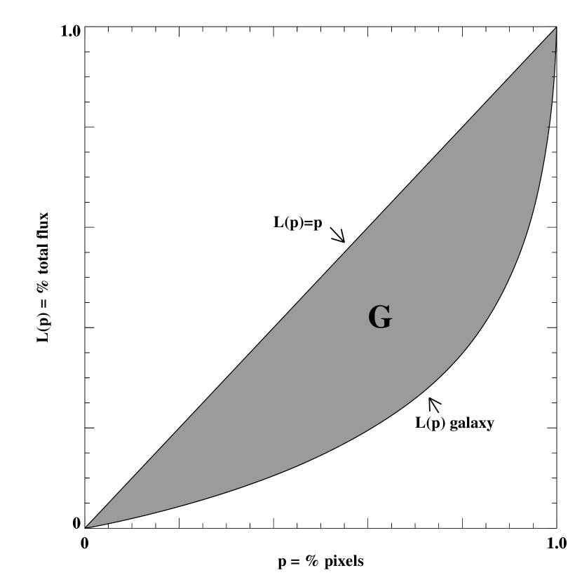
Figure 1: The Lorenz curve – the Gini coefficient is the area between the Lorenz curve of the galaxy’s pixels, and that of equitable distribution (shaded region). The given curve is for S0 NGC4526, G=0.59

where $p$ is the percentage of the poorest citizens or faintest pixels, F(x) is the cumulative distribution function, and $\bar{X}$ is the mean over all (pixel flux) values $X_{i}$ (Lorenz 1905). The Gini coefficient is the ratio of the area between the Lorenz curve and the curve of “uniform equality” where $L(p)=p$ (shaded region, Figure 1) to the area under the curve of uniform equality ($=1/2$). For a discrete population, the Gini coefficient is defined as the mean of the absolute difference between all $X_{i}$:

$$G=\frac{1}{2\bar{X}n(n-1)}\sum^{n}_{i=1}\sum^{n}_{j=1}|X_{i}-X_{j}|$$ (2)

where $n$ is the number of people in a population or pixels in a galaxy. In a completely egalitarian society, $G$ is zero, and if one individual has all the wealth, $G$ is unity. A more efficient way to compute $G$ is to first sort $X_{i}$ into increasing order and calculate

$$G=\frac{1}{\bar{X}n(n-1)}\sum^{n}_{i}(2i-n-1)X_{i}$$ (3)

(Glasser 1962).

For the majority of local galaxies, the Gini coefficient is correlated with the concentration index, and increases with the fraction of light in a compact (central) component. In a study of 930 SDSS Early Data Release galaxies, Abraham et al. (2003) found $G$ to be strongly correlated with both concentration and surface brightness. However, unlike $C$, $G$ is independent of the large-scale spatial distribution of the galaxy’s light. The correlation between $C$ and $G$ exists because highly concentrated galaxies have much of their light in a small number of pixels. High $G$ values may also arise when very bright galaxy pixels are not found in the center of a bulge. Therefore $G$ differs from $C$ in that it can distinguish between galaxies with shallow light profiles (which have both low $C$ and $G$) and galaxies where much of the flux is located in a few pixels not at the projected center (which have low $C$ but high $G$).

In practice, the application of the Gini coefficient to galaxy observations requires some care. One must have a consistent definition of the pixels belonging to the galaxy in order to measure the distribution of flux within those pixels and compare that distribution to other galaxies. The inclusion of “sky” pixels will systematically increase $G$, while the exclusion of low-surface brightness “galaxy” pixels will systematically decrease $G$. Abraham et al. (2003) measure $G$ for galaxy pixels which lie above a constant surface-brightness threshold. This definition makes the direct comparison between high-redshift galaxies and the local galaxy population difficult because of the $(1+z)^{4}$ surface-brightness dimming of distant galaxies. Therefore, we attempt to create a segmentation map of the galaxy pixels in a way that is insensitive to surface-brightness dimming. The mean surface brightness $\mu(r_{p})$ at the Petrosian radius $r_{p}$ is used to set the flux threshold above which pixels are assigned to the galaxy. The Petrosian radius is the radius $r_{p}$ at which the ratio of the surface brightness at $r_{p}$ to the mean surface brightness within $r_{p}$ is equal to a fixed value, i.e.

$$\eta=\frac{\mu(r_{p})}{\bar{\mu}(r<r_{p})}$$ (4)

where $\eta$ is typically set to 0.2 (Petrosian 1976). Because the Petrosian radius is based on a curve of growth, it is largely insensitive to variations in the limiting surface brightness and $S/N$ of the observations. This revised definition should allow better comparison of $G$ values for galaxies with varying surface brightnesses, distances, and observed signal-to-noise..

The galaxy image is sky-subtracted and any background galaxies, foreground stars, or cosmic rays are removed from the image. The mean ellipticity and position angle of the galaxy is measured using IRAF task ellipse. The Petrosian “radius” (or semi-major axis length) is measured for increasing elliptical apertures, rather than circular apertures. While the Petrosian radius determined by the curve of growth within circular apertures is similar to that determined from elliptical apertures for most galaxies, elliptical apertures more closely follow the galaxy’s true light profile and can produce very different $r_{p}$ values for edge-on spirals. To create the segmentation map, the cleaned galaxy image is first convolved with a Gaussian with $\sigma=r_{p}/5$. This step raises the signal of the galaxy pixels above the background noise, making low-surface brightness galaxy pixels more detectable. Then the surface brightness ${\mu}$ at $r_{p}$ is measured and pixels in the smoothed image with flux values $\geq{\mu}(r_{p})$ and less than 10 $\sigma$ from their neighboring pixels are assigned to the galaxy. The last step assures that any remaining cosmic rays or spurious noise pixels in the image are not included in the segmentation map. This map is then applied to the cleaned but unsmoothed image, and the pixels assigned to the galaxy are used to compute the Gini coefficient.

Even when the pixels assigned to a galaxy are robustly determined, the distribution of flux within the pixels will depend on the signal-to-noise ratio ($S/N$) as noise smears out the flux distribution in the faintest pixels. This is illustrated in the left of Figure 2 by adding increasing Poisson sky noise to the S0 galaxy NGC4526 image, and recalculating the segmentation map and Gini coefficient. We define the average signal-to-noise per galaxy pixel $<S/N>$ as

$$<S/N>=\frac{1}{n}\sum^{i}_{n}\frac{S_{i}}{\sqrt{\sigma_{sky}^{2}+S_{i}}}$$ (5)

where $S_{i}$ is pixel $i$’s flux, $\sigma_{sky}$ is the sky noise, and $n$ is the number of galaxy pixels in the segmentation map. As $<S/N>$ decreases, the distribution of measured flux values in the faintest pixels becomes broader. The measured Gini coefficient increases because low surface-brightness galaxy pixels are scattered to flux values below the mean sky level, resulting in negative flux levels for the faintest pixels assigned to the galaxy by our smoothed segmentation map. We note that, while the Poisson noise redistributes all the pixel flux values, the effects are significant only for pixels with intrinsic flux values $\leq 3\sigma_{sky}$. Therefore, as a first order correction, we compute the Gini coefficient of the distribution of absolute flux values:

$$G=\frac{1}{\bar{|X|}n(n-1)}\sum^{n}_{i}(2i-n-1)|X_{i}|$$ (6)

Low-surface brightness galaxy pixels with flux values scattered below the sky level are reassigned positive values (right of Figure 2). This correction recovers the “true” Gini coefficient to within 10% for images with $S/N>2$; at very low $S/N$ values, even the brightest galaxy pixels are strongly affected by noise and the Gini coefficient is not recoverable. In Figures 3-4, we show the final segmentation maps used to compute the Gini coefficient as contour maps for eight galaxies of varying morphological type (Table 1).

2.2 The Moment of Light

The total second-order moment $M_{tot}$ is the flux in each pixel $f_{i}$ multiplied by the squared distance to the center of the galaxy, summed over all the galaxy pixels assigned by the segmentation map:

$$M_{tot}=\sum_{i}^{n}M_{i}=\sum_{i}^{n}f_{i}\cdot((x_{i}-x_{c})^{2}+(y_{i}-y_{c})^{2})$$ (7)

where $x_{c},y_{c}$ is the galaxy’s center. The center is computed by finding $x_{c},y_{c}$ such that $M_{tot}$ is minimized.

The second-order moment of the brightest regions of the galaxy traces the spatial distribution of any bright nuclei, bars, spiral arms, and off-center star-clusters. We define $M_{20}$ as the normalized second order moment of the brightest 20% of the galaxy’s flux. To compute $M_{20}$, we rank-order the galaxy pixels by flux, sum $M_{i}$ over the brightest pixels until the sum of the brightest pixels equals 20% of the total galaxy flux, and then normalize by $M_{tot}$:

$$M_{20}\equiv{\rm log10}\left(\frac{\sum_{i}M_{i}}{M_{tot}}\right) {\rm while} \sum_{i}f_{i}<0.2f_{tot}$$ (8)

Here $f_{tot}$ is the total flux of the galaxy pixels identified by the segmentation map and $f_{i}$ are the fluxes for each pixel $i$, order such that $f_{1}$ is the brightest pixel, $f_{2}$ is the second brightest pixels, and so on. The normalization by $M_{tot}$ removes the dependence on total galaxy flux or size. We find that defining $M$ with brighter flux thresholds (e.g. 5% of f_tot) produce moment values that are unreliable at low spatial resolutions (§2.3), while lower flux threshold lead to a less discriminating statistic.

While our definition of $M_{20}$ is similar to that of $C$, it differs in two important respects. Firstly, $M_{20}$ depends on $r^{2}$, and is more heavily weighted by the spatial distribution of luminous regions. Secondly, unlike $C$, $M_{20}$ is not measured within circular or elliptical apertures, and the center of the galaxy is a free parameter. We shall see in §3 that these differences make $M_{20}$ more sensitive than $C$ to merger signatures such as multiple nuclei. In Figures 3 and 4, we display the segmentation maps and the regions containing the brightest 20% of the flux for the eight test galaxies.

2.3 Concentration, Asymmetry, and Smoothness

Concentration is defined in slightly different ways by different authors, but the basic function measures the ratio of light within a circular or elliptical inner aperture to the light within an outer aperture. We adopt the Bershady et al. (2000) definition as the ratio of the circular radii containing 20% and 80% of the “total flux” :

$$C=5\ \rm{log10}\left(\frac{r_{80}}{r_{20}}\right)$$ (9)

where $r_{80}$ and $r_{20}$ are the circular apertures containing 80% and 20% of the total flux, respectively. For comparison to the most recent studies of galaxy concentration, we use Conselice’s (2003) definition of the total flux as the flux contained within 1.5 $r_{p}$ of the galaxy’s center (as opposed to Bershady’s definition as the flux contained within 2 $r_{p}$). For the concentration measurement, the galaxy’s center is that determined by the asymmetry minimization (see below). In Figures 3-4, we over-plot $r_{80}$ and $r_{20}$ for eight galaxies of varying morphological type in the far left-hand panels.

The asymmetry parameter $A$ quantifies the degree to which the light of a galaxy is rotationally symmetric. $A$ is measured by subtracting the galaxy image rotated by 180 degrees from the original image (Abraham et al. 1995, Wu 1999, Conselice et al. 2000).

$$A=\sum_{i,j}\frac{|I(i,j)-I_{180}(i,j)|}{|I(i,j)|}-B_{180}$$ (10)

where $I$ is the galaxy’s image and $I_{180}$ is the image rotated by 180 about the galaxy’s central pixel, and $B_{180}$ is the average asymmetry of the background. $A$ is summed over all pixels within 1.5 $r_{p}$ of the galaxy’s center. The central pixel is determined by minimizing $A$. The asymmetry due to the noise must be corrected for, and it is impossible to reliably measure the asymmetry for low $S/N$ images. In Figures 3-4, we display the residual $I-I_{180}$ image and the 1.5 $r_{p}$ aperture in the second column. Objects with very smooth elliptical light profiles have a high degree of rotational symmetry. Galaxies with spiral arms are less symmetric, while extremely irregular and merging galaxies are often (but not always) highly asymmetric.

The smoothness parameter $S$ has been recently developed by Conselice (2003), inspired by the work of Takamiya (1999), in order to quantify the degree of small-scale structure. The galaxy image is smoothed by a boxcar of given width and then subtracted from the original image. The residual is a measure of the clumpiness due to features such as compact star clusters. In practice, the smoothing scalelength is chosen to be a fraction of the Petrosian radius.

$$S=\sum_{i,j}\frac{|I(i,j)-I_{S}(i,j)|}{|I(i,j)|}-B_{S}$$ (11)

where $I_{S}$ is the galaxy’s image smoothed by a boxcar of width 0.25 $r_{p}$, and $B_{S}$ is the average smoothness of the background. Like $A$, $S$ is summed over the pixels within 1.5 $r_{p}$ of the galaxy’s center. However, because the central regions of most galaxies are highly concentrated, the pixels within a circular aperture equal to the smoothing length 0.25 $r_{p}$ are excluded from the sum. In Figures 3-4, we display the residual $I-I_{S}$ images, and the 0.25 and 1.5 $r_{p}$ apertures in the third column. $S$ is correlated with recent star-formation (Takamiya 1999, Conselice 2003). However, because of its strong dependence on resolution, it is not applicable to poorly resolved and distant galaxies.

3 RESOLUTION AND NOISE EFFECTS

In order to make a fair comparison of the measured morphologies of different galaxies, we must understand how noise and resolution affect $G$ and $M_{20}$. This is particularly important when comparing local galaxies to high-redshift galaxies, as the observations of distant galaxies are generally of lower signal-to-noise and resolution than those of local galaxies. We have defined $G$ and $M_{20}$ in the previous sections in an attempt to minimize systematic offsets with noise and resolution. Nevertheless, any measurement is ultimately limited by the $S/N$ of the observations. Also, the PSF and finite pixel size of the images may introduce increasing uncertainties to the morphologies as the resolution decreases and small-scale structures are washed out.

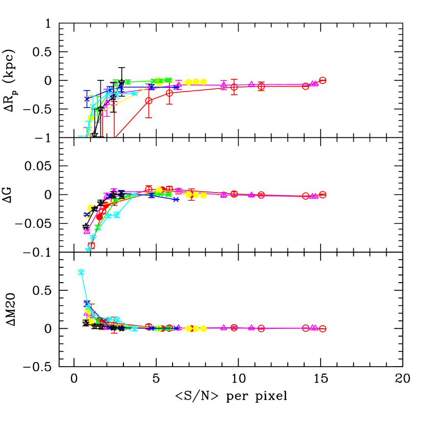
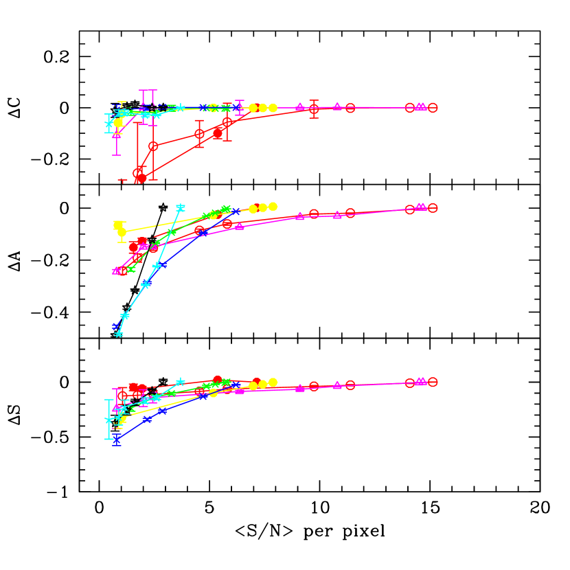
Figure 5: $\Delta r_{p}$, $\Delta$G, $\Delta M_{20}$, $\Delta$C, $\Delta$A, and $\Delta$S vs. $<S/N>$ per pixel. E/NGC5322 = red filled circles, S0/NGC4526= red open circles, Sab/NGC3368= magenta triangles, Sbc/NGC3953= yellow squares, Sc/NGC2403=green crosses, Sd/NGC4713=dark blue crosses, Arp220=light blue stars, SuperAntena=black stars

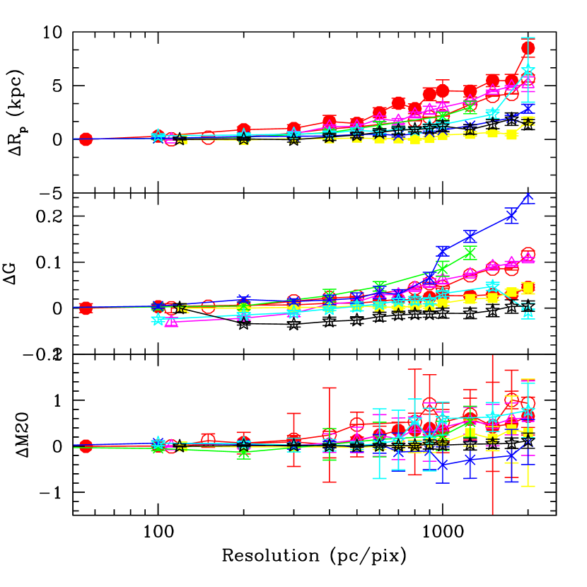
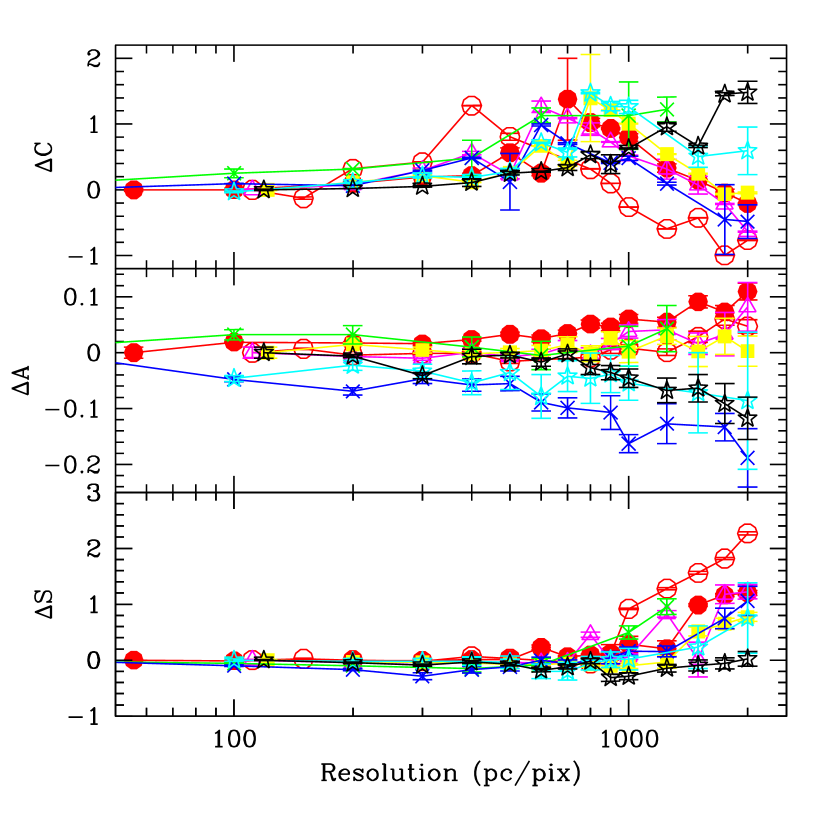
Figure 6: $\Delta r_{p}$, $\Delta$G, $\Delta$M₂₀, $\Delta$C, $\Delta$A, and $\Delta$S vs. resolution (pc per pixel). Symbols are same as Figure 5.

We have chosen eight galaxies of varying morphological type (Figures 3 and 4; Table 1) to independently test the effects of decreasing $S/N$ per pixel and physical resolution (pc per pixel) on the measurements of $G$, $M_{20}$, $C$, $A$, and $S$. For the $S/N$ tests, random Poisson noise maps of increasing variance were added to the original sky-subtracted image. For each noise-added image, we measured $r_{p}$, created a new segmentation map, measured $<S/N>$ for galaxy pixels assigned by the segmentation map, and measured $G$, $M_{20}$, $C$, $A$, and $S$. Noisy galaxy images were created and measured 20 times at each $S/N$ level, and the mean changes in the morphological values with $<S/N>$ are plotted in Figure 5. To simulate the effect of decreasing resolution, we re-binned the galaxy images to increasingly large pixel sizes. Re-binning the original galaxy images increases the $S/N$ per pixel, so additional Poisson sky noise ($\sigma_{sky}$) was added to the re-binned image such that average $<S/N>$ was kept constant with decreasing resolution. Again, we measured $r_{p}$, created a segmentation map, and computed the average change $G$, $M_{20}$, $C$, $A$, and $S$ with resolution for 20 simulations at each resolution step (Figure 6).

We find that $G$, $M_{20}$, and $C$ are reliable to within $\sim$ 10% ($\Delta\leq$ 0.05, 0.2, and 0.3 respectively) for galaxy images with $<S/N>\geq 2$. $A$ systematically decreases with $<S/N>$, but generally shows offsets less than 0.1 at $<S/N>\geq 5$. $S$ also systematically decreases with $<S/N>$, and has decrements less than 0.2 at $<S/N>\geq 5$. Decreasing resolution, however, has much stronger effects on the morphology measurements. $C$ and $M_{20}$ show systematic offsets greater than $\sim$ 15% ($\Delta\geq 0.5$ and 0.3, respectively) at resolution scales worse than 500 pc, as the cores of the observed galaxies become unresolved. $G$, $A$, and $S$, on the other hand, are relatively stable to decreasing spatial resolution down to 1000 pc. As a galaxy’s image becomes less resolved, the observed curve of growth changes resulting in larger $r_{p}$ values, and therefore producing slightly higher $G$ values as the segmentation map grows accordingly. At the lowest resolutions, the observed biases in $C$, $A$ and $S$ appear to be a function of Hubble type: the E-Sbc galaxies are biased to higher $A$ and $S$ and lower $C$, while both the Sd and mergers are biased toward lower $A$ and the merger remnants are biased to higher $C$. On the other hand, on the Sc and Sd galaxies show $G$ offsets $>$ 20% ($\Delta\sim 0.1$) at resolutions between 1000 and 2000 pc.

4 LOCAL GALAXY MORPHOLOGIES

4.1 Frei and SDSS Local Galaxy Samples

We have measured $G$, $M_{20}$, $C$, $A$, and $S$ at both $\sim 4500$Å and $\sim 6500$Å for 104 local galaxies taken from the Frei et al. (1996) catalog. The Frei catalog galaxies are a representative sample of bright, well-resolved, Hubble-type galaxies (E-S0-Sa-Sb-Sc-Sd), and have been used as morphological standards by a number of authors (Takamiya 1999; Wu 1999; Bershady et al. 2000; Conselice et al. 2000; Simard et al. 2002). The galaxies were observed by Frei et al. (1996) with either the 1.5 meter telescope at Palomar Observatory or the 1.1 meter telescope at Lowell Observatory. The Palomar images were taken in the Thuan-Gunn $g$ and $r$ filters ($\lambda_{eff}=$ 5000Å, 6500Å) at plate scale = 1.19 ″ per pixel and typical PSF FWHM $\sim$ 2-3 ″. The Lowell images were taken in the $B_{J}$ and $R$ pass-bands ($\lambda_{eff}$ = 4500Å, 6500Å) at a plate scale = 1.35 ″ per pixel and typical PSF FWHM $\sim$ 3-5 ″. In Table 2, we give $G$, $M_{20}$, $C$, $A$, and $S$ as measured in $R$/$r$ and $B_{J}$/$g$ for each of the galaxies.

We have also obtained the images of 9 Frei galaxies and 44 other galaxies selected by their $u$-band brightness ($u<14$) from the SDSS Data Release 1 database (Abazajian et al. 2003). The morphologies of the SDSS sample were measured in the $u$, $g$ and $r$-bands ($\lambda_{eff}$ = 3600Å, 4400Å, and 6500Å respectively; Table 3). The SDSS plate scale is 0.4″ per pixel and the $r$-band PSF FWHM values are typically $\sim$ 1.3-1.8 ″(Stoughton et al. 2002). We find that the mean absolute difference between the SDSS and Frei observations are :

$$\begin{array}[]{llllll}\delta G=0.02&\delta M_{20}=0.12&\delta C=0.11&\delta A=0.04&\delta S=0.09,&r/R\ {\rm band}\\ \delta G=0.02&\delta M_{20}=0.11&\delta C=0.14&\delta A=0.05&\delta S=0.14,&g/B\ {\rm band}\\ \end{array}$$ (14)

In addition, we have analyzed $B$-band images of 22 nearby dwarf irregular galaxies from the Van Zee (2001) sample (Table 4). We have selected galaxies from the original Van Zee sample with minimal foreground star contamination and $<S/N>$ $\geq$ 2. These images were obtained at the Kitt Peak 0.9 m telescope and have PSF FWHM $\sim$ 1.4-2.3 ″and a plate scale=0.688 ″.

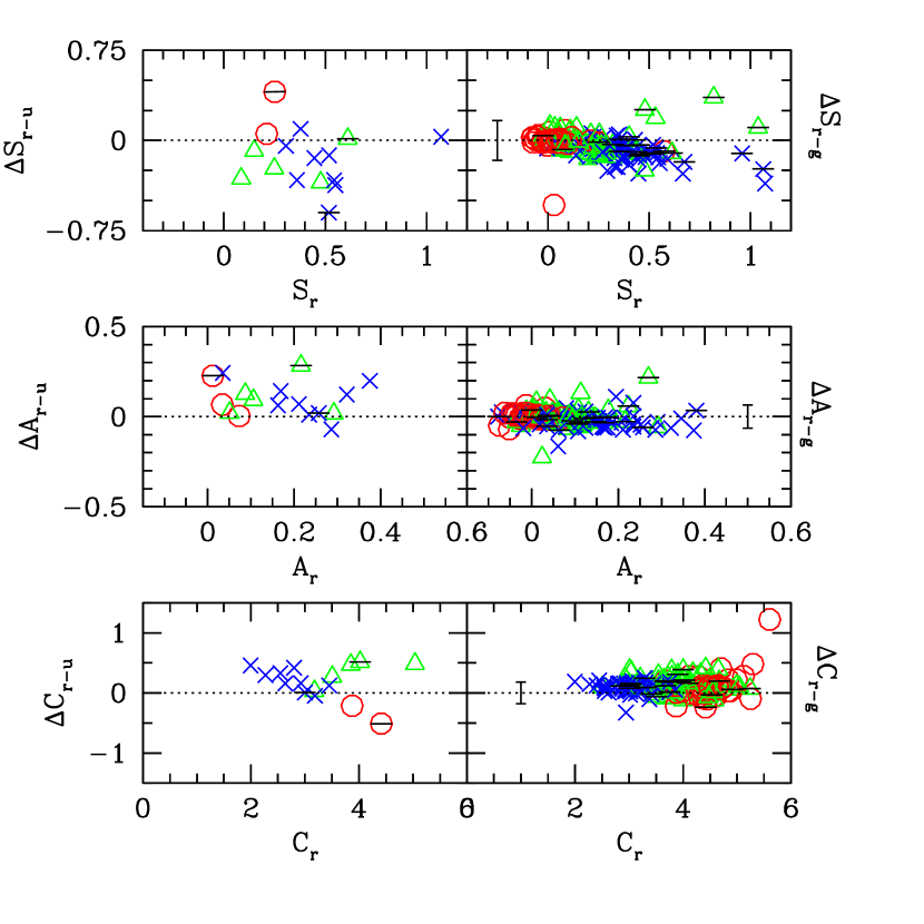
Figure 7: Change in $CAS$ morphology from $\sim$ 6500Å ($R/r$) to $\sim$ 3600Å ($u$) for SDSS u-selected sample with $S/N_{u}>2.0$ (left) and to $\sim$ 4500Å ($B/g$) for Frei and SDSS galaxies with $S/N>2.0$ (right). The error-bars are $\sqrt{(\delta_{r}^{2}+\delta_{g}^{2})}$, where $\delta$ is the average difference between SDSS and Frei et al. observations of the same galaxies. E/S0 are red circles, Sa-Sbc are green triangles, and Sc-Sdm are blue crosses.

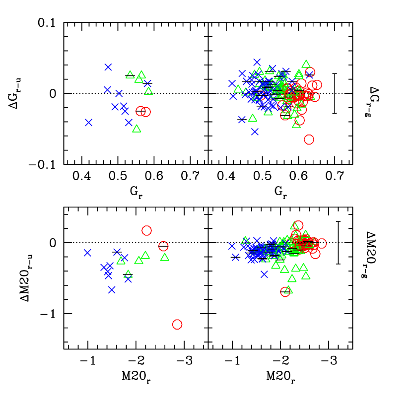
Figure 8: Change in $G$, $M_{20}$ morphology from $\sim$ 6500Å ($R/r$) to $\sim$ 3600Å ($u$) for SDSS u-selected sample with $S/N_{u}>2.0$ (left) and to $\sim$ 4500Å ($B/g$) for Frei and SDSS galaxies with $S/N>2.0$ (right). Error-bars and point symbols are same as Figure 7.

In Figures 7-8, we examine the dependence of $C$, $A$, $S$, $G$, and $M_{20}$ on the observed near-ultraviolet/optical wavelength. For the majority of galaxies, the difference between the observed morphologies at $\sim$ 4500Å ($B/g$)and 6500Å ($R/r$) are comparable to the observational offsets between the SDSS and Frei observations of the same galaxies in the same bandpass. The observed changes in $C$, $G$, and $M_{20}$ from $\sim$ 3600Å ($u$) to $\sim$ 6500Å ($r$) are also consistent with observational scatter. The SDSS $u$-band observations often have too low $S/N$ to obtain reliable asymmetries. This may also produce the increased scatter in $S$. Nevertheless, late-type galaxies generally have higher clumpiness values and slightly higher $M_{20}$ values at 3600 Å than 6500 Å. A handful of galaxies (many of which are edge-on spirals) show much larger morphological changes at bluer wavelengths. The S0 galaxy UGC1597 has an obvious tidal tail, and it has higher $g$-band $A$, $S$, and $G$ values and a lower $g$-band $C$. Several mid-type spirals have significantly higher $M_{20}$ values in $B/g$ than in $R/r$. These include NGC3675, an Sb with prominent dust features, and NGC 5850, an Sb with a star-forming ring.

Previous studies have noted small offsets in concentration and asymmetry from $U$ and $B$ to $R$, with much stronger shifts at wavelengths $\leq$ 2500Å (Brinchmann et al. 1998, Conselice et al. 2000, Kuchinski et al. 2001). We see similar trends of slightly higher $B/g$ asymmetries for late-type spirals ($\sim 0.05$) and lower $B/g$ concentrations for most galaxies ($\sim 0.1$). However, given that these trends are smaller than the difference between different observations of the same galaxy at the same wavelength, we conclude that morphological K-corrections to $C$ and $A$ are not very substantial for most normal galaxies observed redward of rest-frame $\sim 3500-4000$ Å. The late-type spirals show small but systematic trends of stronger clumpiness and higher second order moments at bluer wavelengths.

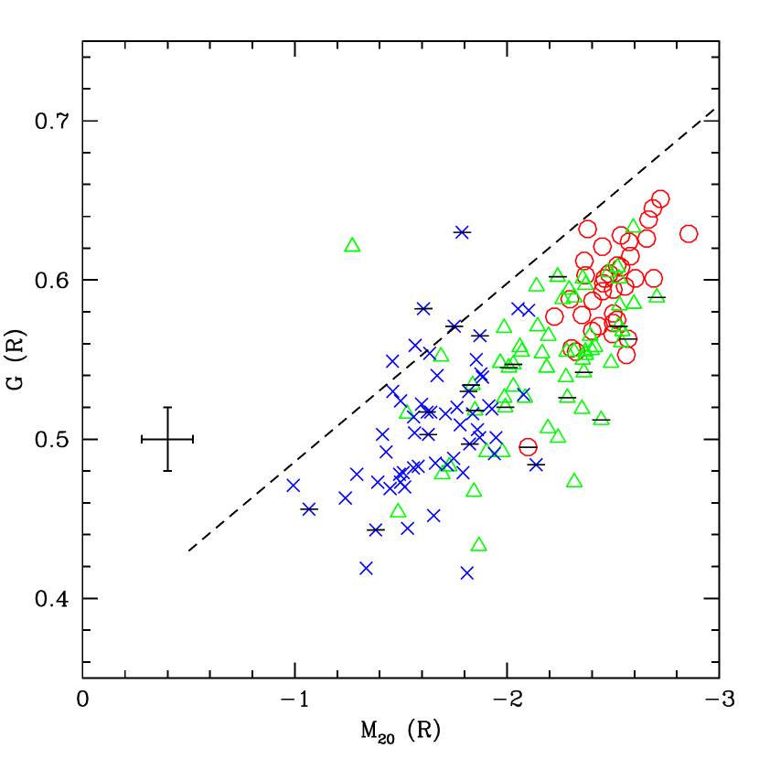
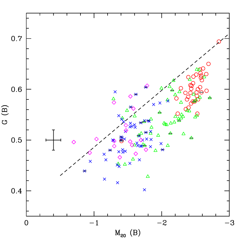
Figure 9: $M_{20}$ v. $G$ for rest-frame $\sim 6500$Å (left) and 4400Å (right) observations of local galaxies (red circles:E/S0, green triangles:Sa-Sbc, blue crosses:Sc-Sd, diamonds:dI, bars:edge-on spirals). The error-bars are mean difference in $G$ and $M_{20}$ between SDSS $r$-band and Frei $R/r$ observations of the same objects. Almost all the “normal” galaxies lie below the dashed line in the $R$-band plot. The outlying Sb galaxy NGC5850 has a strong star-forming ring and is in a close pair with NGC 5846. Three of the outlying dI in the $B$-band plot are star-bursting.

In Figure 9, we examine the $G-M_{20}$ morphologies of local galaxies observed in both the $R/r$ and $B/g$-bands. The distribution of local galaxies is very similar at both wavelengths, with E/S0s showing high $G$ and low $M_{20}$ values, Sa-Sbc at intermediate $G$ and $M_{20}$ values, and most late-type spirals and dI with low $G$ and higher $M_{20}$ values. Most edge-on galaxies (barred symbols) show $G$ and $M_{20}$ values consistent with the mean values for their Hubble type. One notable exception is the S0 NGC4710, which has a prominent dust lane and $G=0.50$, $\sim$ 0.1 lower than for other E/S0s. The majority of local galaxies lie below the rough dividing line plotted in Figure 9. Four out of the 22 dIs lie above this line. Two of these are classified as star-bursting dwarfs (UGC11755 and UGCA439), and a third has the bluest $U-B$ color gradient in the sample (UGC5288; Van Zee 2001). The other outliers are UGC10991 which appears to have a tidal tail and star-forming knots, and UGC10310 which has two very bright knots in its outer arms that may be foreground stars. As we discuss in the next section, most ULIRGs lie above this dividing line. While a few truly star-bursting dIs are $\sim 0.04$ in G above the normal galaxy sequence at blue wavelengths, it appears that dIs will not seriously contaminate the merger/interacting galaxies classified by $G-M_{20}$.

4.2 Merger Indicators

One of the primary goals of morphological studies is to quantitatively identify interacting and merging galaxies. Towards this end, Abraham (1996) and Conselice (2000, 2003) have used combinations of concentration, asymmetry, and smoothness to roughly classify “normal” galaxies as early and late-types, as well as to distinguish mergers from these normal types. Abraham (2003) also found that for a large sample of normal galaxies, the Gini coefficient is strongly correlated with concentration, color, and surface brightness, and therefore may be as efficient as concentration at quantifying galaxy morphologies. Here we compare the effectiveness of our definition of the Gini coefficient (Equation 6) to $C$ at classifying local galaxy types and identifying merger candidates. We also expect that $M_{20}$ will be strongly correlated to $C$, due to their similar definitions, and therefore examine the $G-M_{20}$ correlation and compare it to the $C-G$ relation found by Abraham et al. (2003).

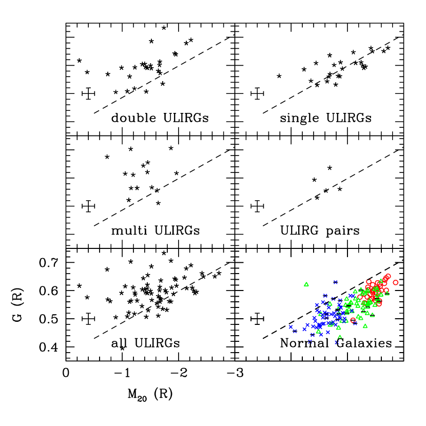
Figure 10: $M_{20}$ v. $G$ for rest-frame $\sim 6500$Å observations of local galaxies (red circles:E/S0, green triangles:Sa-Sbc, blue crosses:Sc-Sd, stars:ULIRGs, bars:edge-on spirals). The error-bars are mean difference in $G$ and $M_{20}$ between SDSS $r$-band and Frei $R/r$ observations of the same objects. Almost all the “normal” galaxies lie below the dashed line.

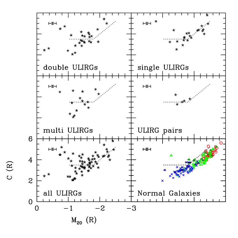
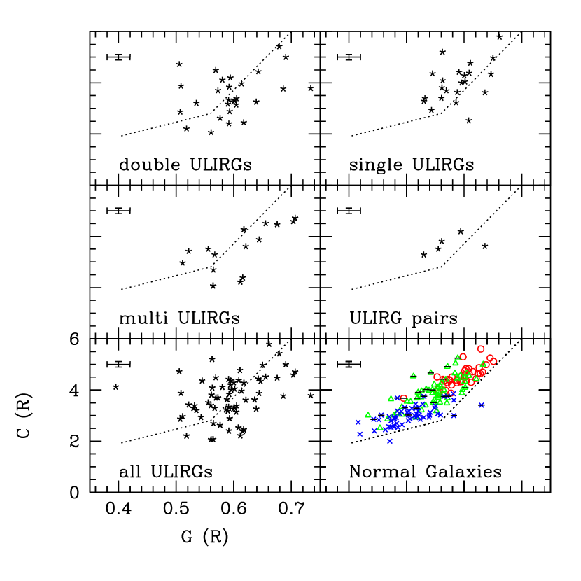
Figure 11: $M_{20}$ v. $C$ and $G$ v. $C$ for rest-frame $\sim 6500$Å observations of local galaxies. Symbols are same as Figure 10. The majority of normal galaxies lie to one side of the dashed lines.

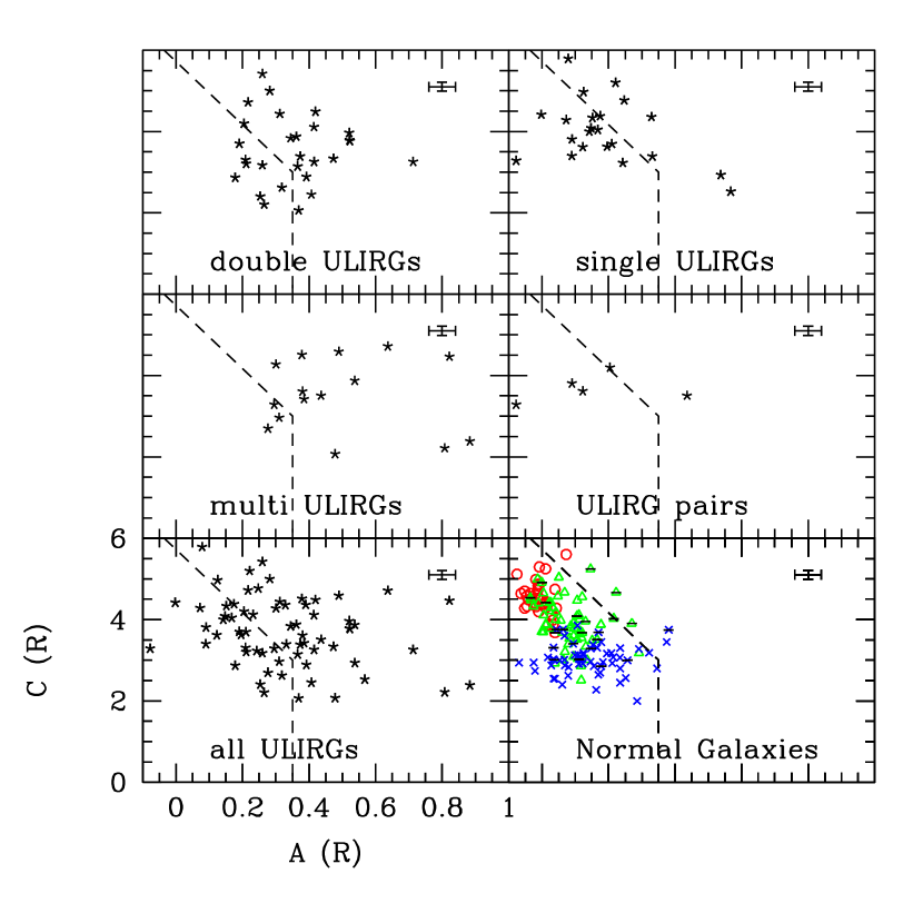
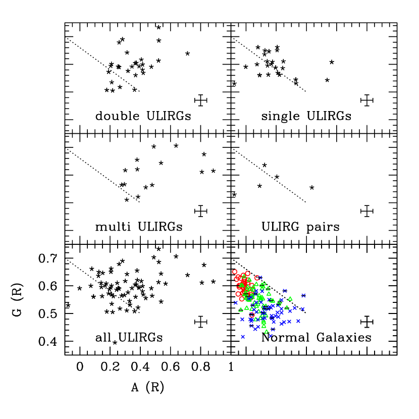
Figure 12: $A$ v. $C$ and $G$ for rest-frame $\sim 6500$Å observations of local galaxies. Symbols are same as Figure 10. The majority of normal galaxies lie to one side of the dashed lines.

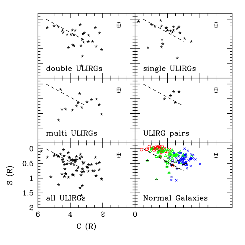
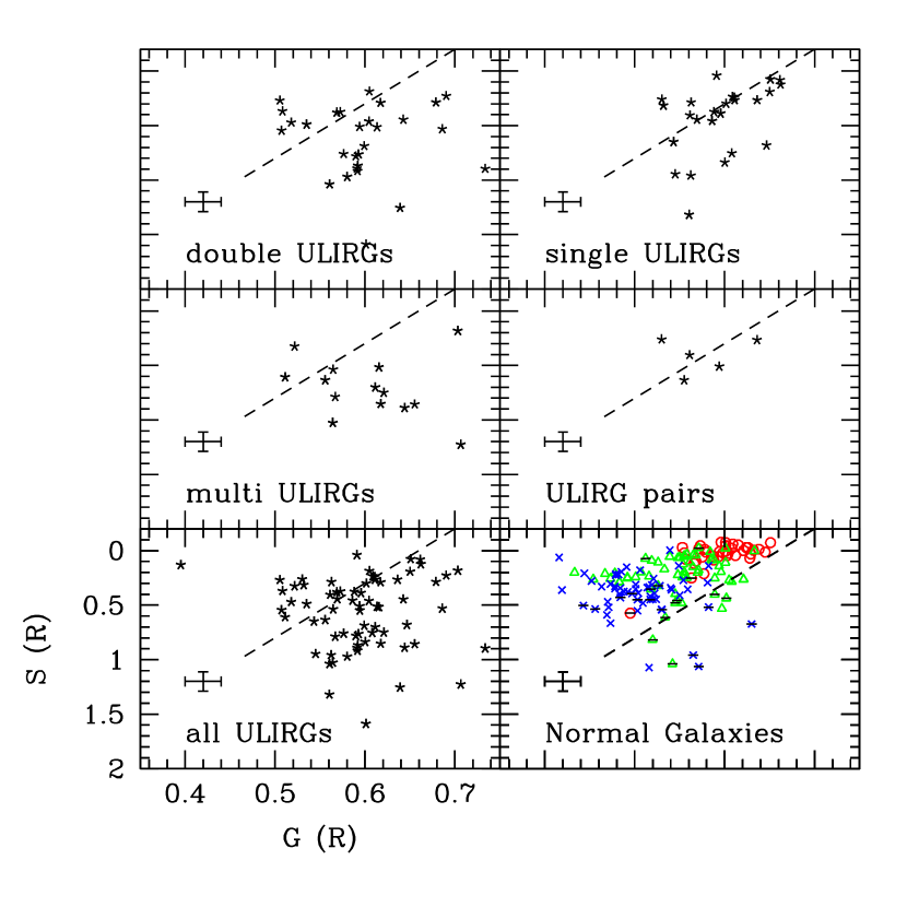
Figure 13: $S$ v. $C$ and $G$ for rest-frame $\sim 6500$Å observations of local galaxies. Symbols are same as Figure 10.

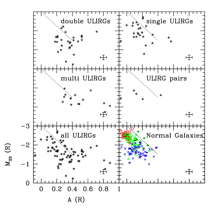
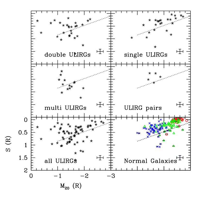
Figure 14: $A$ v. $M_{20}$ and $M_{20}$ v. $S$ for rest-frame $\sim 6500$Å observations of local galaxies. Symbols are same as Figure 10.

In Figures 10-14, we compare the $R/r$-band morphological distributions of our local galaxy sample to archival HST WFPC2 F814W observations of 73 ultra-luminous infrared galaxies with $11.5\leq$ log($L_{FIR}/L_{\odot}$) $\leq 12.5$ and $<S/N>\geq 2$ (ULIRGs; Borne et al. 2000, HST Cycle 6 program 6346, Table 5). ULIRGs often show morphological signatures of on-going or recent merger events in the form of high asymmetries, multiple nuclei, and tidal tails (Wu et al. 1998, Borne et al. 2000, Conselice et al. 2000, Cui et al. 2001). We have divided the ULIRG sample into objects with “single”, “double”, or “multiple” nuclei as classified by Cui et al. 2000 by counting the number of surface brightness peaks with FWHM $>$ 0.14 ″ and $M_{I}<-17.0$ separated by less than 20 kpc projected. We also identify ULIRGs in projected pairs as IRAS sources with projected separations greater than 20 kpc and less than 120 kpc. The ULIRG sample has a mean redshift of $\sim 0.2$, therefore the F814W bandpass ($\lambda_{eff}=$ 8200Å) samples the rest-frame light at $\sim 6800$Å. Given the 0.14 ″ PSF of the WF camera, ULIRGs at $z<0.25$ are spatially resolved to better than $\sim$ 500 pc, and may be directly compared to the local galaxy $r/R$-band observations.

Most ULIRGs lie above the $G-M_{20}$ correlation for normal galaxies (Figure 10, bottom panels), while many ULIRGs overlap with the $C-G$ and $C-M_{20}$ correlations for normal galaxies (Figure 11). Normal local galaxies also segregate more cleanly from the ULIRGs sample in $G-A$ and $G-S$ than $C-A$ and $C-S$ (Figures 12-13). In particular, the Gini coefficient of edge-on spirals galaxies is more consistent with the values obtained for face-on spirals. Also, ULIRGs with double or multiple nuclei generally have higher Gini coefficients relative to their concentrations than most normal galaxies. $G-M_{20}$ is slightly less effective at identifying single-nuclei ULIRGs than $G-A$ and $G-S$; however, $M_{20}$ is a more robust indicator at low $S/N$ than $A$ and $S$ and at low resolution than $S$ (Figures 5-6), and therefore may be applied to fainter galaxy populations. We find that $M_{20}$ in combination with $C$, $A$, and $S$ is not effective at separating the ULIRGs from the normal galaxy population (Figures 12 and 14). In Table 6, we give the results of a series of two-dimensional Kolmogorov-Smirnov (KS) tests (Fasano & Franceschini 1987) applied to the ULIRGs and $R/r$-band normal galaxy observations for each combination of $C$, $A$, $S$, $G$, and $M_{20}$. For all the tests, the probability that the ULIRGs and normal galaxies are drawn from the same parent sample is less than $10^{-6}$.

While the ULIRG population as a whole occupies a different region of $C-A-S-G-M_{20}$ space than our SDSS and Frei galaxy samples, we also find significant differences between ULIRGs in well-separated pairs, ULIRGs with single nuclei, and ULIRGs with double or multiple nuclei (Table 6). ULIRGs in pairs show the smallest offsets from the normal galaxy sample. Double and multi-nuclei ULIRGs show the greatest changes in morphology, with typically large $M_{20}$ and $A$ values. Single-nucleus ULIRGs appear similar to paired ULIRGs, but can also have higher $G$ and $C$. Two dimensional KS tests show that the multi- and double-nuclei ULIRGs are distinct from the single-nucleus ULIRGs and paired ULIRGs with greater than 97% and 90% confidence, respectively. The multi- and double-nuclei ULIRGs have a greater than 5% probability of being drawn from the same sample, while single-nucleus ULIRGs and ULIRGs in pairs have a greater than 12% probability of being drawn from the same sample.

5 GALAXY MORPHOLOGIES AT REDSHIFT $>2$

One of the major successes of the hierarchical paradigm of galaxy formation has been the discovery of large fractions of morphologically-irregular galaxies at $z>1$ (e.g. Driver et al. 1995; Abraham et al. 1996; Odewahn et al. 1996; Abraham & van den Bergh 2001). Many of these galaxies are excellent merger candidates, and suggest merger fractions between 25-40% at $0.5<z<2$. However, morphological studies of the most distant galaxies - the Lyman-break galaxies (LBGs) - have produced confusing and conflicting conclusions. Initial HST WFPC2 observations of the rest-frame far-ultraviolet morphologies of 20 $z>3$ galaxies found that they possessed one or more compact “cores” with sizes similar to present-day spiral bulges (Giavalisco et al. 1996). More recent ACS observations of large numbers of $2<z<6$ LBGs have confirmed ultraviolet half-light radii between 1.5 and 3.5 kpc and concentrations similar to local bulges and ellipticals (Ferguson et al. 2003). However, these LBGs have an ellipticity distribution more like disk galaxies than ellipsoids, leading to the conclusion that LBGs are drawn from a mixture of morphological types. Rest-frame optical observations in the near-infrared with NICMOS have shown that the observed LBG morphologies are not a strong function of wavelength (Papovich et al. 2001; Dickinson 1999), and that LBGs have internal far-UV - optical color dispersions much smaller than $z\sim 1$ galaxies (Papovich 2002). LBGs are significantly bluer than local galaxies, and it is likely that their ultraviolet and optical morphologies are dominated by young stars. Their small sizes, high concentrations, and high star-formation rates suggest that many are precursors to local spiral bulges. However, surface-brightness dimming may prevent the detection of faint tidal tails and some appear to possess multiple nuclei. In a recent study of the optical morphologies of the Hubble Deep Field North galaxies, Conselice et al. (2003) found that 7 out of 18 $z<3$, $M_{B}<-21$ galaxies possess corrected asymmetries greater than 0.35, implying that up to 50% are recent mergers. However, as we found in §4, asymmetry is not as sensitive by itself at detecting merger remnants as it is in combination with $C$ or $G$. Here we re-examine the optical morphologies of the HDFN high-redshift galaxy sample using $C$, $G$, and $M_{20}$, and we attempt to classify these galaxies as ellipticals, disks, or recent mergers.

The Hubble Deep Field North has 27 spectroscopically-confirmed high-redshift galaxies and 70 additional candidates with $1.7<z<4$ and $H<25.0$ (Papovich et al. 2001 and references therein) . At these redshifts, the near-ultraviolet and optical regions of the galaxies spectral energy distributions have been shifted to redward of 1 $\mu$m, and therefore require infrared observations to directly compare their morphologies to the rest-frame near-UV/optical morphologies of local galaxies. The HDFN has been observed with the NICMOS camera 3 in the F110W ($J$) and F160W ($H$) band-passes ($\lambda_{eff}=1.1\mu$m, $1.6\mu$m) down to a 10 $\sigma$ limiting magnitude of 26.5 (Dickinson 1999, HST Cycle 7 program 7817). Most of the HDFN LBGs are fainter than $H=23.0$; therefore, to increase their signal-to-noise per pixel, we have measured the morphologies of the LBG sample in a summed F110W and F160W image. The effective central wavelength of the summed LBG observations is $\sim 1.3\mu$m. Galaxies at $z\sim 2$ and 3 are observed at rest-frame wavelengths 4300Å and 3250Å  respectively. Out of our initial sample of 97 $H<25$ $1.7<z\leq 3.8$ galaxies, 33 galaxies with $1.7<z<2.3$ and 16 galaxies with $2.3\leq z\leq 3.8$ have $<S/N>>2.0$ (Table 7). We also give estimates of the rest-frame $M_{B}$ in AB magnitudes, computed by interpolating between the $J$, $H$, and $K_{s}$ fluxes and assuming $H_{0}=70$ km s^-1 Mpc^-1, $\Omega_{\Lambda}$ = 0.7, $\Omega_{m}$ = 0.3 cosmology.

The NICMOS images offer the highest available resolution at near-UV/optical wavelengths for these galaxies. Nevertheless, the physical resolution of the $z>2$ galaxies is significantly worse than that for the local galaxy images. The dithered NIC3 observations have a pixel scale = 0.08″ per pixel and a PSF FWHM = 0.22 ″. At $z\geq 2$ this corresponds to a physical pixel scale of $\sim 670$ pc and PSF FWHM $\sim$ 1.8 kpc. Our simulations in §3 showed that these resolutions produce strong biases in the measured morphologies which are often a function of morphological type. The well-defined correlations of local galaxy morphologies are likely to change significantly with these biases. Therefore we compare the LBG morphologies to local galaxy images which have been measured from degraded $u$-band and $B/g$-band images. The galaxies are selected to lie in the same $(M_{B}-M^{*})$ range (Figure 15), assuming $M^{*}=-20.1$ locally (Blanton et al. 2003b) and $M^{*}=-22.9$ at $z\geq 2$ (Shapley et al. 2001). This selection tests a “passive” evolutionary scenario, in which the local galaxies were brighter in the past but did not evolve morphologically. We select local galaxies observed in $B/g$ with $3.5\geq(M_{B}-M^{*})\geq 1.0$ to compare to a similarly selected $z\sim 2$ sample, and local galaxies observed in $u$ with $2.5\geq(M_{B}-M^{*})\geq-0.5$ to compare to the $z\sim 3$ sample.

The local galaxies images were first deconvolved in the standard way in IDL: we divide the Fourier transform of the image by the Fourier transform of the PSF, and compute the inverse Fourier transform of the result. Next they were re-binned to the pixel scale of galaxies observed at $z=2$ (670 pc per pixel) or $z=3$ (616 pc per pixel), and convolved with the NIC3 PSF (FWHM = 0.22″= 2.75 pixels). The galaxy fluxes were scaled to the count rate for an $M^{*}$ galaxy at $z=2$ or $z=3$ observed by NICMOS in $F110W$ + $F160W$. Finally, a blank region of NICMOS HDFN combined $F110W$ $+$ $F160W$ image was added to the redshifted galaxy images to simulate the effects of sky noise. (Note that we do not conserve the luminosities of the local galaxy sample. Many local galaxies would not be visible at $z=2-3$ in the rest-frame $u$ or $B$, and Lyman break galaxies are typically two magnitudes brighter than local galaxies. Our simulations in §3 suggest that at $<S/N>>2$, spatial resolution will dominate any morphological biases.)

We find that the poor spatial resolution of $z=2-3$ galaxies is expected to significantly bias their observed morphologies. In Table 8, we give the simulated mean biases in $C$, $A$, $S$, $G$, and $M_{20}$ for early, mid, and late-type galaxies at $z=2$ and $z=3$ observed at $\sim$ 1.3$\mu$m. A scatter of $\sim 0.13$ is introduced to the $A$ measurements, making it ineffective at distinguishing between early and late-type galaxies. $S$ also has large uncertainties at these resolutions, and large biases for E/S0s as a result of their unresolved centers. $C$ and $M_{20}$ are also significantly biased as a function of morphological type, but have a greater dynamical range and therefore are still useful. $G$ remains a reliable unbiased diagnostic out to at least $z\sim 3$ for the NICMOS HDFN plate scale and PSF (Table 8).

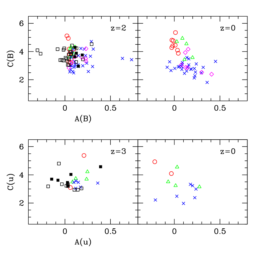
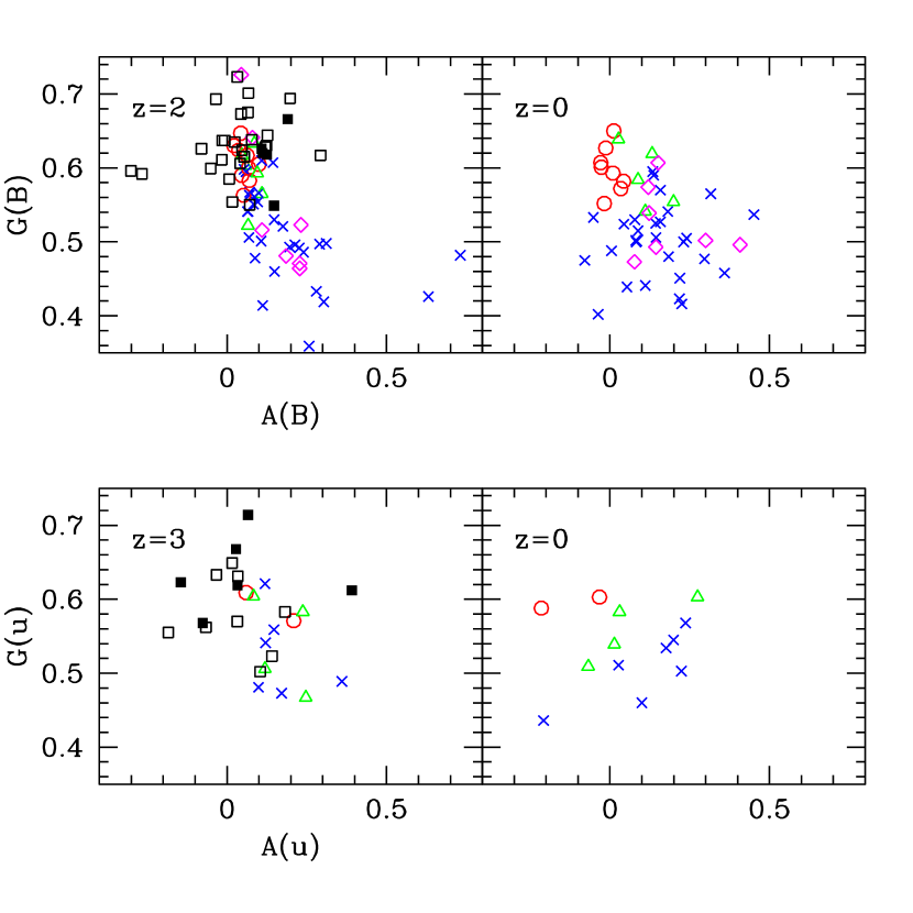
Figure 16: $A$ v. $C$ and $A$ v. $G$ for the HDFN Lyman break galaxies (open squares: LBGs with spectroscopic redshifts, filled squares: LBGs with photometric redshifts). The right hand panels show observed morphologies of normal local galaxies (circles:E/S0, triangles:Sa-Sbc, crosses:Sc-Sd, diamonds:dI). The left hand panels show the observed LBG morphologies and the morphologies of local galaxies expected for z=2-3 galaxies at the NICMOS HDFN image resolution.

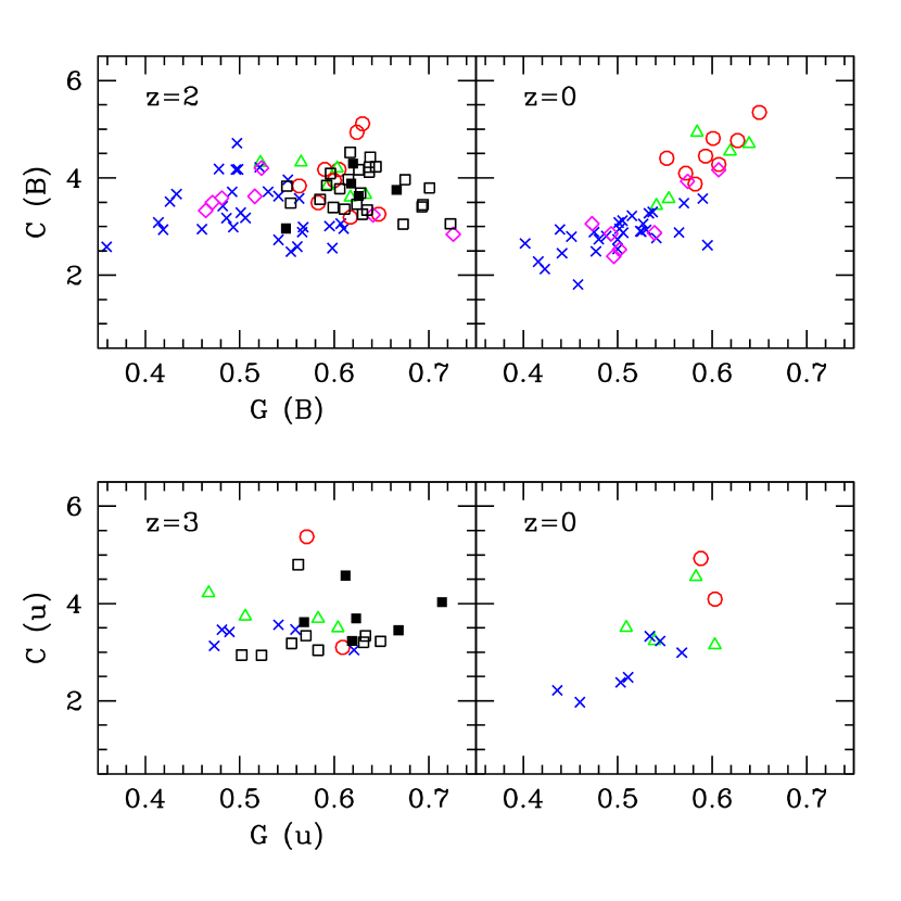
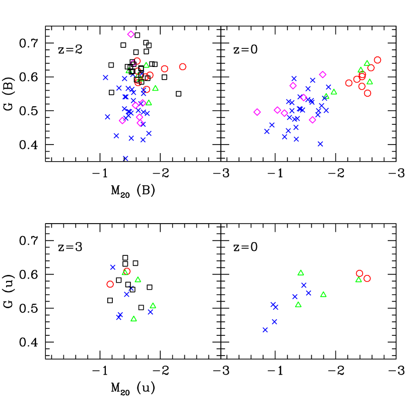
Figure 17: $G$ v. $C$ and $M_{20}$ v. $G$ for the HDFN Lyman break galaxies (symbols are the same as Figure 16).

Given these biases, the some of the observed LBG morphologies appear to be similar to the morphologies of local early-type galaxies (Figures 16-17). However, some of the $z\sim 2-3$ galaxies have higher Gini coefficients and/or asymmetries than expected from the degraded local galaxy images (Figure 16), and one $z\sim 3$ object has a double nucleus, resulting in a much higher asymmetry and $M_{20}$ than any of the degraded local galaxy images. We have applied a series of two-dimensional KS-tests to the LBG sample and degraded local galaxy simulations, similar to the ones used in §4 (Table 9). We find that the $z\sim$ 2 LBG sample has a less than $0.4\%$ probability of matching the degraded $B/g$ band local galaxy morphologies for all combinations of $C-A-G-M_{20}$, except for $C-M_{20}$ where systematic biases are the strongest. The $z\sim 3$ LBGs are more likely to be drawn from a populations of galaxies with “normal” morphologies ($>$ 2% probability); however fewer galaxies are observed in the $z\sim 3$ and the $u$-band local galaxy samples, and one galaxy is highly asymmetric. Therefore, it is highly unlikely that the $z\sim 2$ galaxies have morphologies identical to local elliptical/S0 or spiral galaxies; rather their high $G$ and moderate $A$ values suggest that they are more like the ULIRG population (Figures 10-12).

6 SUMMARY

We have re-defined the Gini coefficient in Equation 6 as a statistic for measuring the distribution of flux values within a galaxy’s image, and introduced $M_{20}$ (Equation 8), the second-order moment of the brightest 20% of the galaxy’s flux. These two indices are complementary, non-parametric morphology measures. We have tested robustness of $G$ and $M_{20}$ to decreasing $S/N$ and resolution and found them to change by less than 10% for average $S/N$ per pixel $\geq$ 2 and resolutions better than 500 pc. At worse resolutions, $C$, $A$, and $M_{20}$ have systematic biases which are a function of Hubble type, while $S$ becomes unreliable. $G$, on the other hand, appears to be remarkably stable at low resolutions and therefore is a powerful tool for classifying the morphologies of high-redshift galaxies.

We have measured $C$, $A$, $S$, $G$, and $M_{20}$ from the near-UV/optical images of 170 local E-S0-Sa-Sb-Sc-Sd-dI galaxies, 73 $z\sim 0.2$ ULIRGs, and 49 $1.7<z<3.8$ Lyman break galaxies. We find that:

1)Normal Hubble-type galaxies follow a tight $G-M_{20}-C$ sequence. Early-type and bulge-dominated systems have high Gini coefficients and concentrations and low second-order moments as a result of their bright and compact bulges. Shallower surface brightness profiles, spiral arms, and off-center star clusters give late-type disks lower Gini coefficients and concentrations and higher second-order moments.

2) In combination with $A$ and $S$, $G$ is more effective than $C$ at distinguishing ULIRGs from normal Hubble types. We also find that most ULIRGs lie above the $G-M_{20}$ sequence and can be identified by by their higher $G$ and $M_{20}$ values. The high Gini coefficients arise from very bright compact nuclei, while multiple nuclei and bright tidal features produce large second-order moments.

3) ULIRGs with double and multiple nuclei have a statistically different distribution in morphology space than single nuclei ULIRGs. ULIRGs with double/multiple nuclei typically have higher second-order moments and asymmetries and slightly lower concentrations than single nuclei ULIRGs. Singly-nucleated ULIRGs are more likely to possess low asymmetries and low second-order moments, and often have higher concentrations and Gini coefficients than ULIRGs in well-separated galaxy pairs.

4) Many of HDFN galaxies at $z\sim 2$ have higher rest-frame $B$-band Gini coefficients and asymmetries than expected for local elliptical and spiral galaxies degraded to the same resolution. Instead, these objects are most similar in morphology to local ULIRGs.

Our revised Gini coefficient has proven itself to be a highly robust and unbiased non-parametric morphological indicator for $z>2$ galaxies observed at HST NICMOS resolution, and therefore has opened a window into the morphologies and assembly of the earliest galaxies. At lower redshifts, and in combination with $M_{20}$, $A$, and $S$, the Gini coefficient allows us to more precisely classify galaxy morphologies and identify merger candidates. In our next paper, we analyze a suite of hydrodynamical galaxy merger simulations to predict the evolution of merging galaxies in G-M-C-A-S morphology space. These simulations will explore a range of merger mass ratios, orbital parameters, and star-formation feedback efficiencies, and will trace the spatial distribution of dark matter, gas, and old and new stars as a function of time (Cox et al. 2004).

We would like to thank T.J. Cox and P. Jonsson for their valuable input and careful reading of this manuscript. We also gratefully acknowledge C. Conselice for his comments and access to his morphology analysis code, M. Dickinson for use of the NICMOS Hubble Deep Field North observations, and the anonymous referee for their useful suggestions. Support for J.L. was provided by NASA through grant number 9515 from the Space Telescope Science Institute, which is operated by AURA, Inc., under NASA contract NAS 5-26555. J.P. acknowledges support from NSF through grant AST-0205944 and NASA through NAG5-12326. P.M. acknowledges support by NASA through grants NAG5-11513 and GO-09425.19A from the Space Telescope Science Institute.

This work is based on observations made with the NASA/ESA Hubble Space Telescope, obtained from the data archive at the Space Telescope Science Institute, and observations from the Sloan Digital Sky Survey. Funding for the Sloan Digital Sky Survey (SDSS) has been provided by the Alfred P. Sloan Foundation, the Participating Institutions, the National Aeronautics and Space Administration, the National Science Foundation, the U.S. Department of Energy, the Japanese Monbukagakusho, and the Max Planck Society. The SDSS is managed by the Astrophysical Research Consortium (ARC) for the Participating Institutions. The Participating Institutions are The University of Chicago, Fermilab, the Institute for Advanced Study, the Japan Participation Group, The Johns Hopkins University, Los Alamos National Laboratory, the Max-Planck-Institute for Astronomy (MPIA), the Max-Planck-Institute for Astrophysics (MPA), New Mexico State University, University of Pittsburgh, Princeton University, the United States Naval Observatory, and the University of Washington.

Table 1: Test Galaxies

Galaxy	Type	Dist	$S/N$	Res	$C_{R}$	$A_{R}$	$S_{R}$	$G_{R}$	$M20_{R}$	notes
		(Mpc)		(pc/pix)
NGC 5332	E4(E/S0)	28.7	7.1	56	4.87	-0.01	-0.03	0.63	-2.66	$-$
NGC 4526	S0_3_(6)	17.0	15.1	111	4.28	0.04	0.05	0.59	-2.40	Virgo Cluster
NGC 3368	Sab(s)II	11.2	14.6	73	3.98	0.06	0.06	0.54	-2.28	Leo Group
NGC 3953	SBbc(r)I-II	18.6	8.4	122	3.54	0.08	0.20	0.51	-2.19	Ursa Major Group
NGC 2403	Sc(s)III	3.2	5.8	19	3.02	0.07	0.34	0.54	-1.67	M81 Group
NGC 4713	SAB(rs)d	17.0	6.4	33	2.56	0.25	0.47	0.47	-1.52	Virgo Cluster
Arp 220	ULIRG	77.0	3.7	37	2.92	0.30	0.43	0.55	-1.64	IRAS15327$+$2340
SuperAntena	ULIRG	245.4	3.1	119	2.06	0.37	1.04	0.56	-1.13	IRAS19254$-$7245

Table 2: Frei Galaxy Catalog

Galaxy	Type	MB	($m-M$)	$S/N_{B}$	CB	AB	SB	GB	M20B	$S/N_{R}$	CR	AR	SR	GR	M20R
NGC 2768	S0_1/2	-20.9	31.75	7.7	4.33	-0.01	0.08	0.59	-2.39	7.9	4.32	-0.02	0.06	0.59	-2.45
NGC 3377	E6	-19.0	30.25	5.6	4.77	-0.01	-0.01	0.63	-2.58	5.0	4.99	-0.02	-0.01	0.64	-2.67
NGC 3379	E1	-19.9	30.12	9.0	4.61	-0.01	-0.02	0.59	-2.52	7.8	4.83	-0.01	-0.02	0.61	-2.54
NGC 4125	E6/S0_1/2	-21.2	31.89	7.1	4.30	0.02	0.04	0.60	-2.28	3.4	4.70	-0.05	0.00	0.63	-2.38
NGC 4365	E3	-21.0	31.55	3.4	4.40	-0.08	-0.06	0.61	-2.43	7.6	4.53	-0.01	0.01	0.59	-2.50
NGC 4374	E1	-21.2	31.32	5.0	4.63	-0.06	-0.08	0.61	-2.46	7.6	4.57	-0.05	-0.05	0.60	-2.46
NGC 4472	E1/S0_1_(1)	-21.7	31.06	9.5	4.22	-0.02	0.00	0.58	-2.37	10.1	4.19	-0.01	-0.01	0.58	-2.35
NGC 4564	E6	-19.0	30.33	6.5	4.81	-0.03	0.03	0.60	-2.44	12.5	5.29	0.01	0.02	0.60	-2.45
NGC 4621	E5	-20.7	31.31	5.3	4.66	-0.04	-0.07	0.63	-2.57	7.2	4.61	-0.02	-0.06	0.61	-2.52
NGC 4636	E0/S0_1_(6)	-20.4	30.83	5.5	4.01	-0.05	-0.04	0.56	-2.40	6.9	4.28	-0.05	-0.01	0.57	-2.43
NGC 5322	E4(E/S0)	-21.3	32.47	5.1	4.83	-0.03	-0.06	0.64	-2.57	3.4	5.12	-0.08	-0.07	0.65	-2.72
NGC 5813	E1	-21.1	32.54	4.7	4.29	-0.03	-0.09	0.58	-2.54	7.3	4.41	-0.02	-0.05	0.57	-2.50
NGC 4340	RSB0_2	-18.6	30.67	5.9	4.40	-0.02	-0.02	0.55	-2.53	6.7	4.51	-0.03	-0.03	0.55	-2.56
NGC 4429	S0_3_(6)/Sa	-19.6	30.57	15.2	3.84	-0.02	-0.01	0.55	-2.24	11.4	4.12	0.03	0.08	0.56	-2.30
NGC 4442	SB0_1_(6)	-18.0	29.41	8.3	4.45	0.01	0.09	0.59	-2.35	15.9	4.36	0.00	0.09	0.59	-2.30
NGC 4477	SB0_1/2_/SBa	-19.7	31.08	7.8	4.49	-0.01	0.02	0.58	-2.46	8.1	4.51	-0.01	0.01	0.58	-2.50
NGC 4526	S0_3_(6)	-20.5	31.14	8.8	4.24	0.04	0.03	0.59	-2.43	15.1	4.28	0.04	0.05	0.59	-2.40
NGC 4710	S0_3_(9)	-19.1	31.03	14.1	3.48	0.03	0.66	0.50	-1.41	27.2	3.68	0.04	0.57	0.50	-2.10
NGC 2775	Sa(r)	-20.4	31.43	8.6	4.01	0.03	-0.01	0.57	-2.29	7.1	4.32	-0.03	-0.02	0.60	-2.36
NGC 3166	Sa(s)	-18.4	29.72	4.7	4.70	0.03	0.033	0.64	-2.52	15.2	4.58	0.05	0.14	0.59	-2.29
NGC 3623	Sa(s)II	-20.1	30.37	8.6	3.99	0.09	0.234	0.55	-2.32	11.4	3.91	0.10	0.20	0.56	-2.37
NGC 4594	SA(s)a	-21.0	29.95	2.0	4.12	-0.02	0.344	0.60	-2.30	6.4	4.00	0.11	0.53	0.60	-2.37
NGC 4754	Sa	-19.6	31.13	4.8	4.87	-0.04	-0.097	0.64	-2.55	8.6	4.99	-0.01	0.00	0.63	-2.60
NGC 4866	Sa	-20.1	32.27	10.0	4.57	-0.01	0.148	0.50	-2.44	9.2	4.53	-0.04	0.07	0.51	-2.44
NGC 5377	SBa or Sa	-19.8	32.04	5.4	4.85	-0.04	-0.065	0.58	-2.48	9.8	4.91	0.00	-0.02	0.57	-2.53
NGC 5701	(PR)SBa	-19.9	31.66	9.0	4.41	0.02	0.075	0.60	-2.26	15.5	4.42	0.03	0.08	0.59	-2.26
NGC 2985	Sab(s)	-20.2	31.38	3.8	4.26	-0.04	-0.113	0.59	-2.47	6.1	4.65	0.00	0.01	0.58	-2.53
NGC 3368	Sab(s)II	-20.0	30.11	8.2	3.80	0.04	-0.003	0.54	-2.19	14.6	3.98	0.06	0.06	0.54	-2.28
NGC 4450	Sab pec	-19.9	30.77	5.2	3.76	-0.01	-0.043	0.54	-2.29	7.6	3.88	0.01	0.06	0.55	-2.36
NGC 4569	Sab(s)I-II	-19.5	29.77	5.6	3.21	0.08	0.182	0.53	-1.85	7.1	3.39	0.08	0.17	0.53	-2.03
NGC 4579	Sab(s)II	-21.0	31.51	6.1	3.93	0.00	0.067	0.56	-2.38	8.0	4.11	0.01	0.06	0.56	-2.40
NGC 4826	Sab(s)II	-20.0	29.37	8.4	2.96	0.12	0.201	0.51	-1.84	6.1	3.21	0.07	0.11	0.53	-1.99
NGC 2683	Sb	-18.8	29.44	14.5	3.57	0.20	0.57	0.55	-1.97	16.1	3.51	0.17	0.46	0.55	-2.03
NGC 3031	Sb(r)I-II	-19.9	27.80	8.4	4.03	0.04	0.02	0.56	-2.41	11.6	4.00	0.04	0.04	0.57	-2.39
NGC 3147	Sb(s)I-II	-22.0	33.40	2.9	3.85	-0.05	-0.07	0.55	-2.29	6.7	4.18	0.04	0.03	0.56	-2.42
NGC 3351	SBb(r)II	-19.5	30.00	7.6	4.11	0.05	0.15	0.55	-2.49	8.0	4.22	0.02	0.07	0.55	-2.49
NGC 3675	Sb(r)II	-20.1	31.11	3.9	3.71	0.25	0.13	0.56	-1.49	7.2	3.77	0.02	0.13	0.55	-2.17
NGC 4157	SAB(s)b?	-19.3	31.48	4.2	3.59	0.05	0.46	0.49	-1.75	13.8	3.90	0.27	0.82	0.52	-1.99
NGC 4192	Sb II	-19.9	30.80	7.2	3.55	0.13	0.45	0.51	-1.66	9.7	3.67	0.12	0.35	0.52	-1.85
NGC 4216	Sb(s)	-20.1	31.13	9.6	5.17	0.15	0.37	0.58	-2.71	11.2	5.24	0.15	0.40	0.59	-2.71
NGC 4258	Sb(s)II	-20.4	29.51	5.7	3.51	0.17	0.26	0.60	-2.00	9.3	3.48	0.15	0.20	0.57	-1.99
NGC 4394	SBb(sr)I-II	-20.2	31.93	5.0	4.44	0.01	0.06	0.58	-2.51	6.6	4.41	-0.01	0.04	0.57	-2.54
NGC 4527	Sb(s)II	-19.3	30.68	7.7	3.77	0.10	0.35	0.51	-2.13	11.2	3.95	0.13	0.32	0.53	-2.28
NGC 4548	SBb(sr)	-20.1	31.05	4.8	3.61	0.02	0.09	0.55	-2.20	5.4	3.71	-0.00	0.05	0.56	-2.32
NGC 4593	SBb(rs)I-II	-21.3	32.93	6.0	4.26	0.01	0.04	0.55	-2.52	6.6	4.29	0.03	0.10	0.56	-2.54
NGC 4725	Sb/SBb(r)II	-20.4	30.46	4.9	3.67	0.01	0.12	0.51	-2.32	6.5	3.69	0.00	0.09	0.52	-2.35
NGC 5005	Sb(s)II	-20.0	30.66	11.9	4.00	0.17	0.38	0.54	-2.25	9.7	4.11	0.11	0.24	0.55	-2.37
NGC 5033	Sb(s)I	-19.7	30.49	2.8	4.56	0.06	0.27	0.61	-2.12	5.4	4.67	0.07	0.27	0.61	-2.48
NGC 5371	Sb(rs)I/SBb(rs)	-21.5	32.81	5.3	2.69	0.07	0.25	0.46	-1.58	7.9	3.04	0.11	0.25	0.49	-1.90
NGC 5746	Sb	-20.7	31.96	10.6	4.47	0.17	0.93	0.54	-2.26	18.5	4.67	0.22	1.04	0.54	-2.36
NGC 5850	SBb(sr)I-II	-21.3	32.81	2.2	4.27	-0.03	0.03	0.58	-2.05	4.3	4.48	-0.03	0.11	0.60	-2.53
NGC 5985	SBb(r)I	-20.9	32.78	2.1	2.75	-0.41	0.16	0.69	-1.79	12.5	2.85	0.12	0.21	0.47	-1.84
NGC 6384	Sb(r)I.2	-20.7	31.88	4.4	3.41	0.09	0.25	0.53	-2.13	6.5	3.79	0.10	0.23	0.56	-2.28
NGC 3344	Sbc(rs)I.2	-19.2	29.62	3.4	3.74	-0.07	0.30	0.62	-2.17	5.8	3.87	0.01	0.20	0.60	-2.14
NGC 3596	Sbc(r)II.2	-19.2	31.16	10.5	2.85	0.15	0.24	0.43	-1.80	14.3	3.00	0.14	0.20	0.43	-1.87
NGC 3631	Sbc(s)II	-20.5	31.48	7.2	3.42	0.17	0.38	0.51	-1.95	7.1	3.64	0.12	0.26	0.47	-2.32
NGC 3726	Sbc(rs)II	-20.6	31.48	5.4	2.41	0.17	0.40	0.45	-1.36	5.6	2.51	0.12	0.26	0.45	-1.49
NGC 3953	SBbc(r)I-II	-20.6	31.48	9.9	3.34	0.15	0.35	0.49	-2.09	8.4	3.54	0.08	0.20	0.51	-2.19
NGC 4013	Sbc	-19.3	31.48	2.3	3.62	-0.13	0.23	0.52	-1.95	3.0	4.00	-0.15	0.48	0.55	-2.01
NGC 4030	SA(s)bc	-19.6	31.60	13.9	3.52	0.13	0.31	0.53	-2.07	12.2	3.80	0.09	0.20	0.56	-2.07
NGC 4123	SBbc(rs)I.8	-19.4	31.39	6.1	2.62	0.10	0.24	0.45	-1.46	5.7	3.01	0.06	0.21	0.48	-1.70
NGC 4501	Sbc(s)II	-20.8	31.20	11.8	3.23	0.16	0.33	0.48	-1.91	13.0	3.34	0.13	0.25	0.49	-1.98
NGC 5055	Sbc(s)II-III	-20.0	30.67	4.7	3.78	0.04	0.19	0.58	-2.09	7.0	3.69	0.06	0.18	0.57	-2.14
NGC 5248	Sbc(s)I-II	-20.1	31.08	5.9	3.24	0.13	0.32	0.49	-1.72	9.6	3.55	0.12	0.24	0.50	-2.24
NGC 2403	Sc(s)III	-18.6	27.54	5.2	2.93	0.08	0.40	0.53	-1.60	5.8	3.0	0.07	0.34	0.54	-1.67
NGC 2541	Sc(s)III	-18.0	30.25	1.9	3.02	-0.05	0.19	0.50	-1.45	2.2	2.1	-0.05	0.24	0.51	-1.63
NGC 2715	Sc(s)II	-19.6	31.41	8.9	3.01	0.19	0.56	0.49	-1.65	10.7	3.2	0.12	0.34	0.48	-1.72
NGC 2903	Sc(s)I-II	-20.1	29.75	10.5	3.05	0.15	0.48	0.53	-1.56	14.0	3.0	0.12	0.39	0.52	-1.60
NGC 3079	Sc(s)II-III	-19.9	31.44	9.1	3.73	0.35	1.07	0.53	-1.69	12.2	3.8	0.38	0.96	0.57	-1.87
NGC 3184	Sc(r)II.2	-18.9	29.30	3.9	2.28	0.23	0.34	0.42	-1.35	4.5	2.4	0.06	0.21	0.44	-1.53
NGC 3198	Sc(s)I-II	-19.8	30.70	4.5	2.99	0.01	0.39	0.54	-1.44	5.2	3.0	0.03	0.35	0.56	-1.57
NGC 3319	SBc(s)II.4	-19.1	30.62	2.0	2.88	-0.08	0.34	0.48	-1.32	2.0	3.0	-0.08	0.35	0.49	-1.43
NGC 3672	Sc(s)I-II	-19.9	32.13	9.0	2.91	0.22	0.42	0.46	-1.67	13.9	3.1	0.21	0.38	0.49	-1.75
NGC 3810	Sc(s)II	-19.4	30.76	10.2	3.30	0.19	0.38	0.49	-1.99	13.4	3.4	0.18	0.32	0.53	-2.08
NGC 3877	Sc(s)II	-19.7	31.48	11.3	3.50	0.17	0.42	0.48	-2.01	18.0	3.7	0.17	0.43	0.48	-2.14
NGC 3893	Sc(s)I.2	-20.1	30.95	13.0	3.13	0.22	0.38	0.52	-1.84	11.5	3.3	0.17	0.26	0.52	-1.91
NGC 3938	Sc(s)I	-19.4	30.31	7.2	2.82	0.19	0.39	0.50	-1.78	9.3	3.0	0.15	0.32	0.52	-1.93
NGC 4088	Sc(s)II-III/SBc	-20.3	31.48	10.2	2.65	0.36	0.94	0.47	-1.15	14.1	2.8	0.35	0.67	0.47	-1.39
NGC 4136	Sc(r)I-II	-18.0	29.70	5.6	2.73	0.08	0.23	0.50	-1.72	6.8	2.9	0.07	0.18	0.51	-1.86
NGC 4178	SBc(s)II	-18.6	30.51	5.1	2.94	0.05	0.60	0.44	-0.86	5.4	3.0	0.04	0.54	0.46	-1.07
NGC 4189	SBc(sr)II	-19.9	32.40	6.9	2.24	0.23	0.55	0.46	-1.18	8.0	2.4	0.24	0.33	0.46	-1.24
NGC 4254	Sc(s)I.3	-20.1	30.56	9.9	3.22	0.32	0.62	0.49	-1.63	11.4	3.3	0.29	0.48	0.51	-1.78
NGC 4487	Sc(s)II.2	-18.6	30.86	3.6	2.80	0.00	0.15	0.49	-1.71	5.4	2.9	0.03	0.21	0.48	-1.79
NGC 4535	SBc(s)I.3	-20.4	30.99	4.7	2.52	0.04	0.40	0.48	-1.43	5.6	2.5	0.04	0.35	0.48	-1.49
NGC 4559	Sc(s)II	-19.9	30.33	5.4	3.13	0.08	0.45	0.54	-1.75	5.9	3.1	0.10	0.36	0.54	-1.88
NGC 4571	Sc(s)II-III	-19.1	30.87	4.0	2.65	-0.04	0.11	0.40	-1.75	4.7	2.7	-0.02	0.06	0.42	-1.81
NGC 4651	Sc(r)I-II	-20.2	31.57	7.4	3.47	0.07	0.19	0.57	-1.97	9.6	3.6	0.07	0.14	0.58	-2.05
NGC 4654	SBc(rs)II-III	-19.5	30.56	5.4	2.75	0.11	0.29	0.48	-1.46	6.5	2.9	0.11	0.22	0.48	-1.56
NGC 4689	Sc(s)II.3	-19.2	30.75	2.7	2.91	-0.09	0.06	0.53	-1.81	3.4	2.9	-0.07	0.00	0.54	-1.88
NGC 4731	SBc(s)III	-19.8	31.65	2.5	3.43	0.12	0.85	0.60	-1.77	2.6	3.4	0.09	0.67	0.63	-1.79
NGC 5334	SBc(rs)II	-19.5	31.48	1.5	2.59	-0.11	0.05	0.43	-1.53	2.2	2.6	-0.10	0.07	0.46	-1.62
NGC 5364	Sc(r)I	-20.1	31.25	4.1	3.03	0.08	0.30	0.49	-1.84	6.4	3.1	0.11	0.35	0.50	-1.95
NGC 5669	SBc(s)II	-19.5	31.48	3.4	2.96	0.10	0.31	0.49	-1.69	5.2	3.1	0.12	0.31	0.50	-1.87
NGC 6015	Sc(s)II-III	-18.7	30.39	6.7	2.90	0.14	0.39	0.53	-1.61	10.8	2.9	0.12	0.33	0.52	-1.71
NGC 6118	Sc(s)I.3	-19.3	31.76	5.1	2.67	0.03	0.25	0.45	-1.53	8.5	2.8	0.08	0.28	0.45	-1.65
NGC 6503	Sc(s)II.8	-13.8	24.66	14.7	3.04	0.17	0.49	0.50	-1.40	20.6	3.3	0.15	0.45	0.52	-1.62
NGC 1156	Im	-17.1	29.46	4.6	2.76	0.18	0.72	0.54	-1.41	7.1	2.9	0.16	0.45	0.52	-1.50
NGC 2976	SdIII-IV	-16.9	27.76	7.5	2.62	0.13	0.48	0.60	-1.31	9.1	2.6	0.08	0.33	0.48	-1.29
NGC 4144	ScdIII	-15.8	27.88	6.0	3.74	0.04	0.64	0.54	-1.80	7.0	3.8	0.04	0.54	0.53	-1.82
NGC 4242	SBdIII	-18.0	29.34	2.1	2.45	0.11	0.21	0.44	-1.22	2.9	2.5	-0.20	0.19	0.49	-1.66
NGC 4449	SmIV	-17.3	27.33	12.1	3.12	0.24	0.48	0.51	-1.42	14.4	3.2	0.21	0.39	0.50	-1.56
NGC 4498	SAB(s)d	-18.9	31.67	4.9	2.95	0.08	0.30	0.50	-1.45	3.7	3.0	0.05	0.34	0.52	-1.56
NGC 4861	SBmIII	-17.5	30.41	2.7	3.27	-0.05	0.20	0.53	-1.54	5.7	2.9	-0.03	0.23	0.48	-1.51
NGC 5204	SdIV	-17.6	29.28	2.5	3.06	0.16	0.26	0.53	-1.22	3.6	3.3	0.24	0.14	0.55	-1.46
NGC 5585	Sd(s)IV	-18.5	29.70	4.5	3.08	0.08	0.19	0.50	-1.84	7.2	3.2	0.20	0.15	0.49	-1.94

Table 3: SDSS u-selected Catalog

Galaxy	Type	MB	($m-M$)	S/Nu	Cu	Au	Su	Gu	M20u	S/Ng	Cg	Ag	Sg	Gg	M20g	S/Nr	Cr	Ar	Sr	Gr	M20r
NGC 3640	E3	-19.0	30.37	1.6	4.26	-0.14	-0.13	0.60	-2.34	6.1	4.55	0.00	0.00	0.63	-2.45	8.3	4.45	0.01	0.00	0.62	-2.45
NGC 4073	E5	-22.2	34.65	0.7	3.95	-0.22	-0.04	0.47	-2.02	2.1	4.51	-0.08	-0.02	0.62	-2.58	2.8	4.64	-0.06	-0.03	0.62	-2.58
NGC 4125	E6/S0_1/2	-21.2	31.89	0.9	4.37	-0.17	-0.11	0.56	-2.36	5.2	4.54	-0.04	0.07	0.63	-2.51	7.1	4.64	-0.04	0.07	0.63	-2.54
NGC 4261	E3	-21.1	32.50	0.9	4.56	-0.07	0.48	0.55	-2.55	4.4	4.64	-0.03	-0.08	0.62	-2.59	6.8	4.71	-0.01	-0.05	0.62	-2.58
NGC 4636	E0/S0_1_(6)	-20.4	30.83	0.6	3.88	-0.23	-0.04	0.46	-1.63	2.9	4.28	-0.06	-0.10	0.60	-2.54	3.9	4.33	-0.05	-0.08	0.60	-2.56
NGC 5322	E4(E/S0)	-21.3	32.47	1.0	4.70	-0.07	0.72	0.57	-2.58	5.4	4.84	-0.01	-0.01	0.63	-2.66	7.1	4.87	-0.01	-0.03	0.63	-2.66
NGC 5813	E1	-21.1	32.54	0.7	4.14	-0.30	-0.76	0.48	-2.26	3.3	4.38	-0.05	-0.10	0.60	-2.57	4.3	4.48	-0.04	-0.08	0.60	-2.60
NGC 1211	(R)SB(r)0/a	-20.0	33.28	0.7	4.35	-0.23	-0.19	0.50	-2.55	5.3	4.35	0.01	0.04	0.62	-2.39	8.2	4.30	0.01	0.05	0.61	-2.36
NGC 2768	S0_1/2_(6)	-18.8	29.44	1.0	3.70	-0.16	0.15	0.53	-2.19	4.2	4.28	-0.03	0.02	0.61	-2.44	5.6	4.36	-0.02	0.02	0.60	-2.48
NGC 3156	S0_2/3_(5)/E5	-18.7	31.75	1.4	4.12	-0.14	-0.01	0.56	-2.37	6.8	4.10	0.03	0.04	0.57	-2.43	8.1	3.87	0.02	0.02	0.56	-2.33
NGC 4036	S0_3_(8)/Sa	-20.3	31.89	1.5	3.80	-0.18	-0.29	0.57	-2.30	10.5	3.96	0.05	0.13	0.56	-2.36	13.6	3.97	0.03	0.10	0.57	-2.40
NGC 4179	S0_1_(9)	-19.4	31.27	1.8	4.19	-0.11	0.06	0.61	-2.43	11.9	4.24	0.01	0.09	0.59	-2.52	17.0	4.38	0.01	0.12	0.57	-2.50
NGC 4624	SB(s)0/a	-19.8	30.25	0.8	4.16	-0.19	0.13	0.50	-2.33	4.1	4.36	-0.03	0.05	0.58	-2.49	5.3	4.38	-0.02	0.06	0.58	-2.52
NGC 4643	SB0_3_/SBa	-19.7	31.38	1.4	4.55	-0.26	-0.67	0.59	-2.28	4.8	4.80	-0.01	0.04	0.64	-2.61	12.4	4.83	-0.01	0.04	0.60	-2.37
NGC 4684	S0_1_(7)	-18.3	30.65	2.2	4.09	-0.03	0.16	0.60	-2.39	9.2	3.87	0.04	0.21	0.58	-2.22	11.4	3.88	0.03	0.21	0.58	-2.22
NGC 5308	S0_1_(8)	-20.0	32.33	2.1	4.93	-0.22	-0.15	0.59	-2.52	12.1	4.65	0.02	0.27	0.59	-2.59	17.1	4.42	0.01	0.25	0.56	-2.57
NGC 5574	S0_1_(8)/a	-18.7	31.89	1.0	5.18	-0.14	0.12	0.60	-2.71	5.7	5.35	0.01	0.02	0.65	-2.69	7.7	5.25	0.01	0.01	0.65	-2.69
NGC 5838	S0_2_(5)	-19.5	31.44	1.0	4.74	-0.26	-0.55	0.57	-2.62	7.2	4.65	0.04	0.01	0.60	-2.66	9.4	4.74	0.04	0.01	0.60	-2.69
UGC 1597	S0; merger?	-22.0	36.30	8.6	3.13	0.07	0.91	0.84	-1.70	8.3	4.38	0.08	0.57	0.69	-2.85	9.8	5.60	0.07	0.03	0.63	-2.86
NGC 2639	Sa	-20.8	33.39	2.4	3.38	-0.04	0.24	0.54	-2.01	8.8	3.84	0.08	0.16	0.59	-2.20	13.1	3.85	0.09	0.15	0.57	-2.20
NGC 3166	Sa(s)	-18.4	29.72	1.3	4.34	-0.12	-0.24	0.62	-2.54	9.1	4.54	0.13	0.20	0.62	-2.42	16.0	4.47	0.11	0.25	0.59	-2.32
NGC 5566	SBa(r)II	-20.2	31.67	1.3	4.42	0.00	0.52	0.58	-2.59	6.8	4.54	0.16	0.33	0.62	-2.63	10.4	4.56	0.12	0.29	0.61	-2.52
NGC 4457	RSb(s)II	-18.7	30.50	2.1	4.55	0.03	0.40	0.58	-2.38	9.7	4.94	0.09	0.13	0.58	-2.56	12.3	5.04	0.05	0.09	0.59	-2.60
NGC 4527	Sb(s)II	-19.3	30.68	0.9	3.16	-0.12	0.87	0.46	-1.35	4.6	3.68	0.14	0.51	0.53	-2.05	6.3	3.88	0.18	0.40	0.55	-2.19
NGC 5806	Sb(s)II.8	-19.0	31.44	1.3	3.05	-0.09	0.53	0.49	-1.20	5.2	3.43	0.11	0.28	0.54	-1.84	6.6	3.60	0.10	0.22	0.55	-1.97
NGC 5850	SBb(sr)I-II	-21.3	32.81	0.5	3.32	-0.24	0.35	0.45	-0.90	2.1	4.00	0.03	0.31	0.58	-1.29	2.6	4.42	0.02	0.26	0.62	-1.27
NGC 5879	Sb(s)II-III	-18.0	30.22	1.5	3.61	-0.10	0.38	0.56	-1.92	2.6	3.93	0.15	0.53	0.60	-2.16	7.0	4.09	0.11	0.44	0.60	-2.24
NGC 7606	Sb(r)I	-21.0	32.52	0.8	3.63	-0.23	0.25	0.45	-1.07	4.8	2.99	0.11	0.40	0.49	-1.60	6.5	3.09	0.10	0.29	0.48	-1.73
NGC 0151	SBbc(rs)II	-21.3	33.64	0.7	3.81	-0.25	0.21	0.45	-1.05	4.1	3.45	0.12	0.46	0.51	-1.67	5.121	3.72	0.12	0.32	0.53	-2.09
NGC 4030	SA(s)bc	-19.6	31.60	2.1	3.24	0.01	0.48	0.54	-1.80	7.7	3.44	0.13	0.37	0.53	-2.04	8.830	3.51	0.11	0.25	0.56	-2.06
NGC 4123	SBbc(rs)I.8	-19.4	31.39	0.8	2.18	-0.13	1.33	0.45	-0.73	2.6	2.67	0.06	0.36	0.54	-1.42	4.442	2.93	0.04	0.23	0.52	-1.53
NGC 4666	SbcII.3	-20.2	31.69	2.0	3.51	-0.07	0.60	0.51	-1.38	7.7	3.81	0.24	0.72	0.54	-1.74	10.705	4.02	0.22	0.61	0.53	-1.84
NGC 5713	Sbc(s) pec	-20.1	32.25	2.3	3.15	0.28	0.83	0.60	-1.42	7.7	3.11	0.35	0.73	0.55	-1.60	8.224	3.18	0.29	0.48	0.55	-1.69
NGC 0701	Sc(s)II-III	-19.0	32.09	1.1	3.25	-0.13	0.36	0.51	-1.23	5.4	2.87	0.14	0.58	0.51	-1.40	6.6	3.03	0.11	0.45	0.50	-1.63
NGC 1035	Sc(s)III	-18.4	31.25	1.6	2.57	-0.10	0.54	0.46	-0.98	6.5	2.74	0.18	0.61	0.48	-1.24	8.4	2.86	0.18	0.50	0.44	-1.38
NGC 1084	Sc(s)II.2	-20.2	31.52	3.4	2.38	0.22	0.92	0.50	-1.01	10.4	2.64	0.29	0.74	0.50	-1.29	11.8	2.80	0.24	0.55	0.50	-1.41
NGC 1087	Sc(s)III.3	-20.2	31.68	1.8	2.36	-0.06	0.05	0.49	-1.17	6.1	2.56	0.24	0.60	0.48	-1.42	6.3	2.69	0.18	0.40	0.48	-1.58
NGC 2537	ScIII pec	-16.7	29.03	3.3	1.54	0.36	0.64	0.47	-0.85	9.4	1.81	0.36	0.56	0.46	-0.95	9.1	2.00	0.29	0.52	0.47	-1.00
NGC 2541	Sc(s)III	-18.0	30.25	0.9	2.39	-0.15	0.79	0.45	-0.72	2.9	2.90	0.04	0.51	0.52	-1.28	1.1	2.97	-0.02	0.37	0.51	-1.32
NGC 3055	Sc(s)II	-19.4	32.09	1.8	2.99	0.10	0.67	0.54	-1.34	6.0	2.87	0.28	0.53	0.52	-1.46	6.6	3.06	0.23	0.42	0.52	-1.64
NGC 4041	Sc(s)II-III	-20.0	31.89	1.7	3.67	0.05	0.61	0.59	-1.96	6.5	3.80	0.19	0.55	0.58	-2.09	8.3	3.85	0.11	0.29	0.58	-2.10
NGC 4273	SBc(s)II	-20.3	32.66	2.2	3.23	0.20	0.59	0.55	-1.55	7.7	3.17	0.39	0.61	0.51	-1.67	8.1	3.18	0.32	0.45	0.52	-1.76
NGC 4409	Sc(s)III	-19.0	31.91	2.4	2.48	0.03	0.28	0.51	-0.97	8.2	2.54	0.23	0.52	0.50	-1.28	8.8	2.64	0.17	0.38	0.49	-1.43
NGC 4605	Sc(s)III	-15.7	26.57	2.3	2.77	0.14	0.88	0.57	-1.14	8.1	2.87	0.28	0.69	0.55	-1.37	8.6	2.93	0.21	0.54	0.53	-1.46
NGC 4630	Sc(s)III	-17.0	30.11	1.5	3.61	0.11	0.85	0.58	-1.90	4.0	3.48	0.16	0.51	0.57	-1.88	4.8	3.38	0.15	0.41	0.55	-1.86
NGC 4653	Sc(rs)I.3	-20.1	32.87	0.8	2.61	-0.16	0.62	0.44	-0.92	2.7	2.95	0.06	0.37	0.53	-1.53	2.7	3.07	0.02	0.27	0.55	-1.64
NGC 4808	Sc(s)III	-17.9	30.23	0.4	2.54	-0.13	-0.47	0.46	-1.05	8.1	2.79	0.22	0.58	0.45	-1.34	9.1	2.96	0.18	0.47	0.47	-1.52
NGC 4900	SB(rs)c	-18.8	30.71	2.7	1.97	0.10	0.69	0.46	-0.99	7.3	2.13	0.22	0.52	0.42	-1.16	7.4	2.27	0.16	0.36	0.42	-1.34
NGC 5334	SBc(rs)II	-19.5	31.48	2.3	2.22	-0.21	0.35	0.44	-0.83	5.4	2.42	0.02	0.35	0.45	-1.37	2.9	2.55	0.04	0.31	0.47	-1.50
NGC 6207	Sc(s)III	-18.3	30.43	2.6	3.33	0.18	1.04	0.53	-1.33	8.7	3.30	0.45	1.43	0.54	-1.82	9.5	3.45	0.38	1.07	0.52	-1.84
NGC 6239	SBcIII pec	-17.7	30.60	2.3	2.99	0.24	1.12	0.57	-1.47	6.0	2.88	0.32	0.63	0.57	-1.54	5.5	3.00	0.26	0.52	0.58	-1.61
NGC 3044	Scd(on edge)	-18.9	31.33	1.3	3.48	-0.33	-1.71	0.57	-1.254	4.8	3.57	0.14	1.30	0.59	-1.62	5.5	3.76	0.06	1.06	0.57	-1.75
NGC 4713	SAB(rs)d	-17.7	29.84	1.8	2.27	0.09	0.69	0.50	-1.080	6.2	2.49	0.30	0.74	0.48	-1.37	6.4	2.56	0.25	0.59	0.47	-1.45
NGC 4771	SAd?	-18.1	31.05	1.1	3.13	-0.17	0.46	0.47	-1.497	4.5	3.22	0.09	0.44	0.52	-1.77	6.1	3.31	0.04	0.39	0.50	-1.82

Table 4: Van Zee Dwarf Irregular Galaxy Sample

Galaxy	Type	$M_{B}$	S/NB	CB	AB	SB	GB	M20B
UGC00290	Sdm	-14.48	2.1	3.75	0.03	0.30	0.54	-1.78
UGC00634	SABm	-17.67	2.5	2.85	0.14	0.61	0.49	-1.15
UGC00685	SAm	-14.74	5.0	2.81	0.18	0.39	0.52	-1.47
UGC00891	SABm	-15.53	3.1	2.90	0.06	0.38	0.49	-1.56
UGC01104	Im	-16.08	9.2	3.18	0.20	0.36	0.50	-1.69
UGC01175	Sm	-14.13	3.8	2.84	0.24	0.27	0.47	-1.38
UGC03647	IBm	-17.06	2.0	2.87	0.12	0.56	0.54	-1.47
UGC04117	IBm	-14.86	4.7	2.89	0.28	0.67	0.48	-0.94
UGC05205	SBm pec	-16.29	4.5	2.72	0.23	0.28	0.48	-1.77
UGC05288	Sdm	-14.44	4.2	3.32	0.13	0.43	0.59	-1.54
UGC09219	Im	-16.33	5.1	2.78	0.36	0.57	0.50	-1.53
UGC09240	IAm	-14.60	5.1	2.54	0.24	0.55	0.50	-1.30
UGC10054	SBdm	-18.13	3.6	3.06	0.08	0.45	0.47	-1.62
UGC10310	SB(s)m	-16.81	3.7	2.39	0.41	1.29	0.50	-0.70
UGC10351	Sdm	-16.06	5.9	3.29	0.15	0.34	0.56	-1.58
UGC10445	SBc	-17.53	4.7	2.53	0.30	0.73	0.50	-1.04
UGC10991	Im	-16.35	2.3	2.68	0.41	0.78	0.54	-1.08
UGC11755	BCD/E	-17.14	9.1	4.17	0.15	0.39	0.61	-1.79
UGC12713	S0/a	-14.76	6.7	2.96	0.18	0.31	0.53	-1.47
UGCA009	IB(s)m	-14.17	3.0	2.69	0.01	0.34	0.49	-1.30
UGCA015	IB(s)m	-12.93	2.4	2.49	0.10	0.47	0.47	-1.09
UGCA439	BCD	-16.73	17.5	3.93	0.12	0.29	0.57	-1.30

Table 5: Borne et al. 2000 ULIRG HST Survey

Galaxy	redshift	RA	DEC	S/N	$C$	$A$	$S$	$G$	$M_{20}$	Nuclei
IRAS00091$-$0738	0.118	00 11 43	$-$07 22 07	2.0	3.63	0.20	0.38	0.59	$-$1.91	Single∗
IRAS00104$-$0139	0.163	00 13 04	$-$01 23 05	2.1	2.20	0.26	0.47	0.52	$-$1.22	Double
IRAS00161$-$0850	0.109	00 18 43	$-$08 33 36	3.7	2.69	0.28	0.54	0.56	$-$1.26	Multiple
IRAS00207+1029	0.231	00 23 22	$+$10 46 22	3.3	3.79	0.52	0.90	0.73	$-$1.74	Double
IRAS00335$-$2732	0.069	00 36 01	$-$27 15 35	5.0	4.33	0.15	0.68	0.65	$-$2.11	Single
IRAS00456$-$2904	0.11	00 48 07	$-$28 48 19	3.9	3.31	0.21	1.59	0.60	$-$1.66	Double∗
IRAS01031$-$2255	0.187	01 05 37	$-$22 39 18	2.0	4.12	0.23	0.13	0.40	$-$1.00	Single
IRAS01199$-$2307	0.156	01 22 21	$-$22 52 07	2.2	4.72	0.22	0.27	0.51	$-$0.89	Double∗
IRAS01284$-$1535	0.153	01 30 53	$-$15 19 51	3.6	3.70	0.19	0.37	0.57	$-$1.67	Double∗
IRAS01579$-$1925	0.173	02 00 18	$-$19 11 00	3.9	4.29	0.07	0.84	0.60	$-$2.27	Single∗
IRASF02130$-$1948	0.192	02 15 24	$-$19 34 27	2.5	3.39	0.37	0.18	0.60	$-$1.40	Double∗
IRAS02459$-$0233	0.18	02 48 28	$-$02 21 35	3.2	2.62	0.32	0.76	0.58	$-$0.38	Double
IRAS04024$-$8303	0.14	03 57 11	$-$82 55 16	5.2	5.20	0.22	0.96	0.56	$-$0.79	Single
IRAS04384$-$4848	0.203	04 39 51	$-$48 43 15	2.1	3.42	0.38	0.33	0.52	$-$1.12	Multiple
IRAS05116+7745	0.157	05 19 12	$+$77 48 12	2.5	2.52	0.57	0.75	0.61	$-$1.44	Single
IRAS05120$-$4811	0.163	05 13 24	$-$48 07 58	2.8	2.87	0.18	0.55	0.51	$-$1.43	Double
IRAS05233$-$2334	0.172	05 25 27	$-$23 32 08	2.8	4.04	0.17	0.30	0.60	$-$1.76	Single
IRAS06206$-$6315	0.092	06 21 01	$-$63 17 23	2.6	3.17	0.26	0.78	0.59	$-$1.52	Double
IRAS06268+3509	0.170	06 30 13	$+$35 07 50	2.2	2.41	0.25	0.92	0.59	$-$0.99	Double
IRAS06361$-$6217	0.16	06 36 36	$-$62 20 32	2.7	4.36	0.33	0.95	0.55	$-$1.35	Single
IRAS06487+2208	0.144	06 51 46	$+$22 04 30	3.0	3.77	0.52	0.53	0.69	$-$1.52	Double
IRAS07246+6125	0.137	07 29 12	$+$61 18 53	2.1	5.79	0.08	0.08	0.66	$-$2.42	Single
IRAS08201+2801	0.168	08 23 13	$+$27 51 39	3.2	3.26	0.42	0.69	0.60	$-$1.50	Double
IRAS08235+1334	0.137	08 26 19	$+$13 24 40	2.3	4.42	0.00	0.04	0.59	$-$2.29	Single∗
IRAS08344+5105	0.0967	08 38 04	$+$50 55 09	2.1	3.97	0.52	0.51	0.61	$-$1.67	Double
IRAS08509$-$1504	0.135	08 53 16	$-$15 15 48	6.8	3.69	0.21	0.44	0.57	$-$1.69	Single
IRAS09039+0503	0.125	09 06 34	$+$04 51 28	3.1	4.44	0.31	0.45	0.64	$-$1.93	Double
IRAS09320+6134	0.0394	09 35 52	$+$61 21 11	3.0	4.09	0.15	0.29	0.56	$-$1.83	Single
IRAS09425+1751	0.128	09 45 21	$+$17 37 54	3.0	6.34	0.21	0.12	0.66	$-$2.72	Single
IRAS10122+4943a	0.154	10 15 21	$+$49 28 19	3.0	3.81	0.09	0.40	0.56	$-$1.87	Single/pair
IRAS10122+4943b	0.154	10 15 21	$+$49 28 19	2.1	3.28	$-$0.08	0.26	0.53	$-$1.46	Single/pair
IRAS12108+3157	0.207	12 13 20	$+$31 40 53	2.1	4.77	0.25	0.24	0.61	$-$2.24	Single
IRAS12112+0305	0.0733	12 13 46	$+$02 48 41	2.0	3.34	0.47	0.89	0.59	$-$1.44	Double
IRAS12202+1646	0.181	12 22 47	$+$16 29 45	3.0	4.97	0.12	0.19	0.65	$-$2.44	Single
IRASF12450+3401	0.159	12 47 32	$+$33 44 35	2.0	2.06	0.64	0.99	0.64	$-$0.97	Multi∗
IRAS12490$-$1009	0.101	12 51 41	$-$10 25 26	3.1	3.88	0.36	0.37	0.51	$-$1.09	Double
IRAS13156+0435b	0.113	13 18 11	$+$04 19 12	2.3	4.20	0.20	0.51	0.59	$-$1.41	Double/pair∗
IRAS13352+6402	0.237	13 36 51	$+$63 47 04	2.1	4.49	0.42	0.38	0.57	$-$0.75	Double
IRAS13428+5608	0.0378	13 44 42	$+$55 53 11	2.2	3.21	0.21	0.49	0.54	$-$1.72	Double
IRAS13442+2321	0.142	13 46 39	$+$23 06 21	2.0	4.13	$-$0.03	0.14	0.58	$-$2.11	Single
IRAS13469+5833	0.158	13 48 40	$+$58 18 52	2.3	3.28	0.30	0.79	0.57	$-$1.53	Double
IRAS13539+2920	0.108	13 56 10	$+$29 05 36	2.1	4.51	0.38	0.86	0.66	$-$1.45	Multiple
IRAS14060+2919	0.117	14 08 19	$+$29 04 46	2.7	4.36	0.39	0.55	0.59	$-$1.78	Multiple
IRAS14170+4545	0.152	14 18 59	$+$45 32 12	2.2	4.38	0.17	0.24	0.61	$-$2.15	Single
IRAS14202+2615	0.159	14 22 31	$+$26 02 06	2.0	3.62	0.12	0.27	0.64	$-$1.69	Single/pair
IRAS14337$-$4134	0.182	14 36 58	$-$41 47 11	2.0	3.49	0.22	0.33	0.58	$-$1.53	Single
IRAS14378$-$3651	0.068	14 40 59	$-$37 04 33	2.9	4.00	0.14	0.39	0.60	$-$2.32	Single
IRAS14575+3256	0.113	14 59 37	$+$32 44 58	4.3	3.61	0.38	0.75	0.62	$-$1.45	Multiple
IRAS15250+3609a	0.0552	15 26 59	$+$35 58 38	5.3	3.51	0.44	0.64	0.56	$-$1.62	Multi/pair∗
IRAS16541+5301	0.194	16 55 20	$+$52 56 36	2.4	2.89	0.39	0.76	0.59	$-$1.23	Double
IRAS17208$-$0014	0.0428	17 23 22	$-$00 17 00	3.9	2.97	0.31	0.61	0.51	$-$1.64	Multiple∗
IRAS18580+6527	0.176	18 58 14	$+$65 31 29	2.3	4.47	0.82	2.45	0.68	$-$0.73	Multiple
IRAS19254$-$7245	0.061	19 31 22	$-$72 39 20	3.1	2.06	0.37	1.04	0.56	$-$1.13	Double
IRAS20100$-$4156	0.13	20 13 30	$-$41 47 34	3.1	2.07	0.48	1.03	0.56	$-$1.16	Multiple
IRAS20176$-$4756	0.178	20 21 11	$-$47 47 07	2.3	3.40	0.09	1.32	0.56	$-$1.67	Single
IRAS20253$-$3757	0.18	20 28 38	$-$37 47 09	2.3	4.59	0.49	0.18	0.70	$-$1.15	Multiple
IRAS20314$-$1919	0.152	20 34 18	$-$19 09 12	2.2	3.14	0.37	0.46	0.60	$-$1.36	Double
IRAS20414$-$1651	0.087	20 44 18	$-$16 40 16	3.5	3.23	0.24	0.46	0.59	$-$1.23	Single
IRAS20551$-$4250	0.043	20 58 27	$-$42 39 03	3.9	4.11	0.41	0.97	0.58	$-$1.64	Double
IRAS21130$-$4446	0.093	21 16 19	$-$44 33 40	3.1	2.38	0.88	0.52	0.62	$-$1.05	Multiple
IRAS22206$-$2715	0.131	22 23 29	$-$27 00 03	2.0	3.87	0.54	0.89	0.64	$-$1.38	Multiple
IRAS22491$-$1808	0.078	22 51 49	$-$17 52 24	2.1	4.72	0.64	1.23	0.71	$-$1.87	Multiple
IRAS22509$-$0040	0.0582	22 53 33	$-$00 24 43	3.8	4.28	0.30	0.85	0.62	$-$1.97	Multiple∗
IRAS22546$-$2637	0.164	22 57 24	$-$26 21 13	2.0	2.99	0.58	0.90	0.58	$-$1.29	Double
IRAS23128$-$5919	0.0446	23 15 47	$-$59 03 14	4.8	2.45	0.41	0.29	0.62	$-$0.24	Double
IRAS23140+0348	0.220	23 16 35	$+$04 05 17	3.0	6.58	0.21	0.08	0.65	$-$2.65	Single
IRAS23146$-$1116	0.101	23 17 14	$-$11 00 37	3.0	3.84	0.34	0.87	0.59	$-$1.45	Double
IRAS23220+2919	0.240	23 24 28	$+$29 35 39	2.7	5.42	0.26	0.29	0.68	$-$2.14	Double
IRAS23230$-$6926	0.106	23 26 04	$-$69 10 19	3.6	2.93	0.54	0.65	0.54	$-$1.64	Single
IRAS23242$-$0357	0.189	23 26 50	$-$03 41 06	2.5	6.00	0.14	0.27	0.61	$-$1.88	Single
IRAS23365+3604	0.0645	23 39 01	$+$36 21 08	3.0	3.39	0.33	0.31	0.53	$-$1.79	Single
IRAS23410+0228	0.0912	23 43 40	$+$02 45 04	3.7	3.26	0.71	1.25	0.64	$-$1.95	Double
IRAS23515$-$2421	0.153	23 54 10	$-$24 04 25	2.6	2.22	0.81	0.70	0.61	$-$1.19	Multiple

Table 6: Two-Dimensional KS Test Probabilities

“Normal” Galaxies v. ULIRGs
	$A$	$S$	$G$	$M_{20}$
$C$	6.6e-15	9.3e-8	7.5e-7	8.3e-8
$A$	…	2.1e-16	7.7e-18	6.2e-14
$S$	…	…	1.6e-13	5.1e-10
$G$	…	…	…	5.8e-13
Double v. Multi-Nuclei ULIRGs
	$A$	$S$	$G$	$M_{20}$
$C$	0.29	0.25	0.15	0.66
$A$	…	0.047	0.17	0.086
$S$	…	…	0.086	0.36
$G$	…	…	…	0.18
Paired v. Single-Nuclei ULIRGs
	$A$	$S$	$G$	$M_{20}$
$C$	0.25	0.21	0.29	0.14
$A$	…	0.51	0.49	0.13
$S$	…	…	0.47	0.30
$G$	…	…	…	0.12
Double+Multi- v. Single-Nuclei ULIRGs
	$A$	$S$	$G$	$M_{20}$
$C$	8.2e-7	0.0012	0.029	3.3e-4
$A$	…	7.1e-6	7.2e-6	9.3e-7
$S$	…	…	0.0024	3.2e-5
$G$	…	…	…	7.6e-4
Double+Multi-Nuclei v. Paired ULIRGs
	$A$	$S$	$G$	$M_{20}$
$C$	0.0041	0.017	0.078	0.057
$A$	…	0.0042	0.020	0.0070
$S$	…	…	0.096	0.016
$G$	…	…	…	0.056

Note. — Two-dimensional K-S test probabilities that two galaxy populations have the same distribution in a two-parameter space.

Table 7: HDFN Lyman Break Galaxies

ID	redshift	RA (J2000)	DEC (J2000)	$H$	MB	rp (″)	$S/N$	$C$	$A$	$G$	$M_{20}$
882	1.8	12:36:45.66	62:12:41.9	22.27	-21.6	0.62	8.2	4.4	0.08	0.64	$-$1.86
1118	1.8	12:36:51.28	62:12:33.8	24.47	-19.7	0.31	4.0	3.3	0.12	0.63	$-$1.45
1217	1.8	12:36:45.15	62:12:05.5	24.77	-19.5	0.41	3.1	3.5	0.02	0.55	$-$1.19
121	1.9	12:36:44.85	62:14:06.1	23.14	-20.9	0.36	4.2	4.0	0.07	0.68	$-$1.77
653	1.9	12:36:56.64	62:13:39.9	23.87	-20.3	0.63	4.0	4.0	0.05	0.62	$-$1.52
769	1.9	12:36:52.00	62:13:14.9	24.86	-19.5	0.48	3.5	3.5	0.05	0.62	$-$1.68
1550	1.9	12:36:58.29	62:12:16.5	23.75	-20.3	0.48	3.4	4.2	-0.08	0.63	$-$1.68
539	2.0	12:36:50.29	62:13:29.8	23.74	-20.5	0.39	3.5	4.1	-0.02	0.64	$-$1.91
697	2.0	12:36:53.78	62:13:25.4	24.17	-20.3	0.43	4.1	3.6	0.01	0.59	$-$1.69
901	2.0	12:36:42.41	62:12:32.5	24.03	-20.5	0.32	3.6	3.1	0.04	0.67	$-$1.60
1128	2.0	12:36:45.42	62:12:13.6	22.12	-23.0	0.47	10.2	3.3	0.29	0.85	$-$1.94
1211	2.0	12:36:48.63	62:12:15.8	22.16	-21.9	1.12	5.5	5.1	0.16	0.63	$-$1.86
1293	2.0	12:36:49.60	62:12:12.7	24.29	-20.2	0.53	3.4	4.2	0.13	0.64	$-$1.54
1582	2.0	12:36:49.12	62:11:50.6	23.85	-20.6	0.46	4.1	4.1	$-$0.27	0.59	$-$1.61
110	2.005	12:36:48.30	62:14:16.6	22.52	-21.9	0.47	6.7	4.1	0.28	0.68	$-$1.62
109	2.009	12:36:48.23	62:14:18.5	23.49	-21.1	0.47	4.7	3.9	0.13	0.62	$-$1.49
1513	2.05	12:37:00.07	62:12:25.3	23.06	-21.0	0.51	6.0	3.0	0.15	0.55	$-$1.38
178	2.1	12:36:52.85	62:14:23.3	24.39	-20.1	0.36	2.9	3.4	0.20	0.69	$-$1.39
254	2.1	12:36:45.39	62:13:50.1	24.45	-20.1	0.26	2.6	3.4	$-$0.04	0.69	$-$1.81
1215	2.1	12:36:51.86	62:12:25.6	24.14	-20.4	0.86	2.7	4.2	$-$0.01	0.64	$-$1.56
1315	2.1	12:36:51.61	62:12:17.3	23.81	-20.7	0.45	3.9	3.8	0.07	0.70	$-$1.76
1433	2.1	12:36:45.42	62:11:48.9	24.41	-20.1	0.43	3.1	3.8	0.04	0.61	$-$1.68
77	2.2	12:36:52.05	62:14:34.0	24.95	-19.7	0.40	2.5	4.1	$-$0.30	0.60	$-$1.79
756	2.2	12:36:55.70	62:13:26.9	24.49	-20.2	0.31	2.8	3.1	0.03	0.72	$-$1.62
937	2.2	12:36:42.87	62:12:27.8	24.66	-20.1	0.38	2.1	3.4	$-$0.05	0.60	$-$2.07
1034	2.2	12:36:43.3	62:12:18.3	24.75	-20.0	0.48	4.2	3.8	0.07	0.55	$-$2.30
1047	2.2	12:36:49.56	62:12:36.0	23.48	-21.2	0.38	5.1	3.7	0.12	0.63	$-$1.50
1179	2.2	12:36:51.32	62:12:27.3	24.17	-20.6	0.62	2.9	4.5	0.29	0.62	$-$1.54
1262	2.2	12:36:52.48	62:12:24.7	24.89	-19.9	0.34	2.9	3.3	0.02	0.64	$-$1.19
1530	2.2	12:36:45.31	62:11:38.5	24.44	-20.1	0.30	2.4	3.4	$-$0.02	0.61	$-$3.05
503	2.233	12:36:55.06	62:13:47.1	23.94	-20.8	0.39	4.6	3.8	0.19	0.67	$-$1.43
274	2.237	12:36:50.09	62:14:01.1	23.58	-21.0	0.55	3.3	4.3	0.11	0.62	$-$1.68
67	2.267	12:36:44.07	62:14:10.1	23.86	-21.0	0.43	4.3	3.6	0.11	0.63	$-$1.48
272	2.4	12:36:50.66	62:14:03.2	24.25	-20.7	0.36	3.1	3.3	$-$0.03	0.63	$-$1.59
502	2.4	12:36:55.15	62:13:48.2	24.49	-20.5	0.35	3.7	3.2	$-$0.03	0.63	$-$1.42
758	2.4	12:36:41.85	62:12:43.6	23.68	-21.2	0.67	4.7	2.9	0.10	0.50	$-$1.68
561	2.419	12:36:54.61	62:13:41.4	24.67	-20.3	0.32	2.9	3.2	0.13	0.64	$-$1.43
741	2.489	12:36:53.18	62:13:22.7	23.99	-21.1	0.39	4.3	3.5	0.03	0.67	$-$1.76
989	2.500	12:36:44.64	62:12:27.4	22.61	-22.5	0.53	4.1	4.0	0.07	0.71	$-$2.00
62	2.6	12:36:43.55	62:14:09.0	23.95	-21.2	0.31	4.3	3.2	0.02	0.65	$-$1.42
782	2.8	12:36:45.0	62:12:51.1	23.20	-20.6	0.55	3.5	3.0	0.18	0.58	$-$1.31
1357/8	2.803	12:36:45.41	62:11:53.1	23.21	-23.1	1.19	5.6	4.6	0.39	0.61	$-$0.90
1541	2.980	12:36:48.31	62:11:45.8	24.51	-21.1	0.39	2.5	3.6	$-$0.08	0.57	$-$1.48
661	2.991	12:36:53.42	62:13:29.4	24.15	-21.0	0.37	3.0	3.2	0.03	0.62	$-$1.30
980	3.0	12:36:52.24	62:12:52.2	24.93	-20.7	0.34	2.9	2.9	0.14	0.52	$-$1.17
521	3.2	12:36:43.96	62:13:11.9	24.61	-21.2	0.56	2.3	4.8	$-$0.07	0.56	$-$1.82
749	3.4	12:36:48.78	62:13:05.8	24.75	-21.5	0.34	3.1	3.3	0.03	0.57	$-$1.47
825	3.475	12:36:39.6	62:12:30.4	24.07	-22.3	0.39	3.0	3.7	$-$0.15	0.62	$-$1.76
1320	3.8	12:36:53.14	62:13:31.7	24.97	-22.0	0.38	2.5	3.2	$-$0.18	0.56	$-$1.54

Table 8: z=2 and z=3 morphological simulations

Type	N	$C_{z}-C_{z=0}$	$A_{z}-A_{z=0}$	$S_{z}-S_{z=0}$	$G_{z}-G_{z=0}$	$M20_{z}-M20_{z=0}$
z=2, rest-frame $B/g$ observations
E/S0	36	+0.14 $\pm$ 0.69	+0.07 $\pm$ 0.05	+0.29 $\pm$ 0.19	-0.01 $\pm$ 0.02	+0.54 $\pm$ 0.26
Sa-Sbc	58	+0.36 $\pm$ 0.51	+0.08 $\pm$ 0.15	+0.05 $\pm$ 0.22	-0.01 $\pm$ 0.03	+0.23 $\pm$ 0.41
Sc-Sd	58	+0.46 $\pm$ 0.37	+0.03 $\pm$ 0.18	-0.10 $\pm$ 0.28	-0.01 $\pm$ 0.04	-0.06 $\pm$ 0.20
dI	22	+0.07 $\pm$ 0.66	-0.07 $\pm$ 0.12	+0.46 $\pm$ 0.53	+0.10 $\pm$ 0.07	-0.16 $\pm$ 0.28
z=3, rest-frame $u$ observations
E/S0	3	+0.04 $\pm$ 0.74	+0.09 $\pm$ 0.23	+0.56 $\pm$ 0.52	-0.02 $\pm$ 0.10	+0.95 $\pm$ 0.40
Sa-Sbc	5	+0.50 $\pm$ 0.72	+0.11 $\pm$ 0.13	-0.10 $\pm$ 0.31	-0.02 $\pm$ 0.03	-0.08 $\pm$ 0.49
Sc-Sd	8	+0.47 $\pm$ 0.58	-0.02 $\pm$ 0.13	-0.34 $\pm$ 0.40	+0.02 $\pm$ 0.07	-0.29 $\pm$ 0.30

Table 9: Lyman Break Galaxy KS Test Probabilities

	$z=2$ LBGs v. local galaxies				$z=3$ LBGs v. local galaxies
	$A$	$G$	$M_{20}$		$A$	$G$	$M_{20}$
$C$	5.1e-4	4.6e-6	0.075		0.065	0.032	0.27
$A$	…	2.1e-8	0.0039		…	0.017	0.13
$G$	…	…	6.6e-6		…	…	0.10

Note. — Two-dimensional K-S test probabilities that two galaxy populations have the same distribution in a two-parameter space.

Figure 2: The pixel flux value distribution as a function of the average signal-to-noise per galaxy pixel for S0 galaxy NGC4526. Left: As $<S/N>$ decreases, more faint galaxy pixels are scattered below the background sky level. Right: The corrected Gini coefficients are calculated from the distribution of absolute pixel flux values.

Figure 3: [Lotz.fig3.gif] Test galaxy morphological measurements $C$, $A$, $S$, $G$, and $M_{20}$ for rest-frame $\sim 6500$Å images (Table 1). In the first panel, inner and outer circles enclose 20% and 80% of the flux within 1.5 $r_{p}$. The second panel shows the residual $I-I_{180}$ image, with the circle at 1.5 $r_{p}$. The third panel shows the residual $I-I_{S}$ image, with the inner and outer circles at 0.25 and 1.5 $r_{p}$. The fourth panel images are the original galaxy images scaled such that the minimum surface brightness matches that used to create the galaxy segmentation maps. The outer edge of the segmentation map are the outer contour plotted in the fourth and fifth panels. The inner contours plotted in the fifth panel trace each galaxy’s brightest 20% of it flux, while the crosses indicate each galaxy’s center. The final panel plots each galaxy’s $G$ and $M_{20}$ where the solid line is for reference.

Figure 4: [Lotz.fig4.gif] Same as Figure 3

Figure 15: $M_{B}-M^{*}$ histograms for the $z\sim 2$ and $B/g$-band local galaxy samples (top) and the $z\sim 3$ and $u$-band local galaxy samples (bottom). $M^{*}$ is assumed to be $-20.1$ for the local galaxies and $-22.9$ for the $z\geq 2$ galaxies.

References

- (1) Abraham, R. G., Valdes, F., Yee, H.K.C., & van den Bergh, S., 1994, ApJ, 432, 75
- (2) Abraham, R.,G., Tanvir, N. R., Santiago, B. X., Ellis, R. S., Glazebrook, K., & van den Bergh, S. 1996, MNRAS, 279, 47
- (3) Abraham, R. G., & van den Bergh, S. 2001, Science, 293, 1273
- (4) Abraham, R., van den Bergh, S., & Nair, P. 2003, ApJ, 588, 218
- (5) Abazajian, K. et al. 2003, AJ, 126, 2081
- (6) Balcells, M., Graham, A., Dominguez-Palmero, L., & Peletier, R. 2003, ApJ, 582, L79
- (7) Bershady, M., Jangren, A., & Conselice, C. 2000, AJ, 119, 2645
- (8) Blanton, M., et al. 2003a, ApJ, 594, 186
- (9) Blanton, M., et al. 2003b, ApJ, 592, 819
- (10) Borne, K. D., Bushouse, H., Lucas, R. A., & Colina, L. 2000, ApJ, 529, 77L
- (11) Brinchmann, J. et al. 1998, ApJ, 499, 112
- (12) Budavari, T., Szalay, A., Connolly, A., Csabai, I, & Dickinson, M. 2000, AJ, 120, 1588
- (13) Carollo, M. 1999, ApJ, 523, 566
- (14) Cohen, J., Hogg, D., Blanford, R., Cowie, L., Hu, E., Songaila, A., Shopbell, P., & Richberg, K. 2000, ApJ, 538, 29
- (15) Conselice, C., Bershady, M., & Jangren, A. 2000, ApJ, 529, 886
- (16) Conselice, C. 2003, ApJS, 147, 1
- (17) Conselice, C., Bershady, M., Dickinson, M., & Papovich, C. 2003, ApJ, 126, 1183
- (18) Cox, T.J., et al. 2004, in preparation
- (19) Cui, J., Xia, X.-Y., Deng, Z.-G., Mao, G., & Zou, Z.-L. 2001, AJ, 122, 63
- (20) Dickinson, M., 1999, in After the Dark Ages: When Galaxies were Young (the Universe at 2 z 5). ed. S. Holt & E. Smith (College Park, Maryland: American Institute of Physics Press), p. 122
- (21) Driver, S. P., Windhorst, R. A., & Griffiths, R. 1995, ApJ, 453, 48
- (22) Eastman, R.G., Schmidt, B.P.& Kirshner, R. 1996, ApJ, 466, 911
- (23) Drozdovsky,I.O. & Karachentsev, I.D. 2000, A&AS, 142, 425
- (24) Fasano, G. & Franceschini, A., 1987, MNRAS 225, 155
- (25) Ferguson, H. C., et al. 2004, ApJ, 600L, 107
- (26) Frei, Z., Guhathakurta, P., Gunn, J, & Tyson, J.A. 1996, AJ, 111, 174
- (27) Freedman, W.L. et al. 2001, ApJ, 553, 47
- (28) Garcia, A.M., Fournier, A., di Nella, H., & Paturel, G. 1996, A&A, 310, 412
- (29) Gavazzi, G., Boselli, A., Scodeggio, M., Pierini, D., & Belsole, E. 1999, MNRAS, 304, 595
- (30) Giavalisco, M., Steidel, C. C., & Macchetto, F. D., 196, 470, 189
- (31) Glasser, G.J. 1962, J. Amer. Stat. Assoc. 57, 648, 654
- (32) Isserstedt, J. & Schindler, R. 1986, A&A, 167, 11
- (33) Jensen, J.B. et al. 2003, ApJ, 583, 712
- (34) Kelly, B.C. & McKay, T.A. 2004, AJ, 127, 625
- (35) Karachentsev, I., Musella, I., & Grimaldi, A. 1996, A&A 310, 722
- (36) Karachentsev, I., et al. 2002, A&A, 383, 125
- (37) Karachentsev, I., & Drozdovsky, I.O. 1998, A&AS, 131, 1
- (38) Kuchinski, L. E., Madore, B.F., Freedman, W.L., & Trewhela, M. 2001, ApJ, 122, 729
- (39) Larsen, S. S. & Richtler, T. 1999, A&A, 345, 59L
- (40) Lorenz, M.O. 1905, Amer. Stat Assoc., 9, 209
- (41) Naim, A., Ratnatunga, K., & Griffiths, R. 1997, 476, 510
- (42) Odewahn, S.C., Windhorst, R.A., Driver, S.P., & Keel, W. 1996, ApJ, 472, L13
- (43) Papovich, C., Dickinson, M., & Ferguson, H.C., 2001, ApJ 559, 630
- (44) Papovich, C., 2002, PhD thesis, Johns Hopkins University
- (45) Parodi, B.R, Saha, A., Sandage, A., & Tammann, G.A. 2000, ApJ, 540, 634
- (46) Peng, C. Y., Ho, L.C., Impey, C.D., & Rix, H.-W. 2002, AJ, 266, 293
- (47) Petrosian, V. 1976, ApJ, 209, L1
- (48) Pierce, M.J. 1994, ApJ, 430, 53
- (49) Pierce, M.J., McClure, R.D., & Racine, R. 1992, ApJ, 393, 523
- (50) Pierce, M.J., & Tully, R.B. 1988, ApJ, 330, 579
- (51) Refregier, A. 2003, MNRAS, 338, 35
- (52) Russell, D.G. 2002, ApJ, 565, 681
- (53) Sandage, A., & Bedke, J. 1994, The Carnegie Atlas of Galaxies: Volume I
- (54) Schade, D., Lilly, S.J., Crampton, D., Hammer, F., LeFevre, 0., & Tresse, L. 1995, ApJ, 451, 1L
- (55) Schoniger, F. & Sofue, Y. 1994, A&A, 283, 21
- (56) Shanks, T. 1997, MNRAS, 290, 77
- (57) Shapley, A., Steidel, C.C., Adelberger, K.L., Dickinson, M., Giavalisco, M., & Pettini, M. 2001, ApJ, 562, 123
- (58) Simard, L., et al. 2002, ApJS, 142, 1
- (59) Takamiya, M. 1999, ApJS, 122, 109
- (60) Theureau, G., Hanski, M., Ekholm, T., Bottinelli, L., Gouguenheim, L., Paturel, G., Teerikorpi, P., 1997, A&A, 322, 730
- (61) Van Zee, L. 2001, AJ, 121, 2003
- (62) Wu, H., Zou, Z. L, Xia, X. Y., & Deng, Z. G. 1998, A&AS, 132, 181)
- (63) Wu, K. 1999, PhD thesis, U.C. Santa Cruz
- (64) Yasuda, N., Fukugita, M., Okamura, S. 1997, ApJS, 108, 417