Non-minimal coupling, exponential potentials and the $w<-1$ regime of dark energy

Abstract

Recent observations and theoretical considerations have motivated the study of models for dark energy with equation of state characterized by a parameter $w=p/\rho<-1$. Such models, however, are usually believed to be inviable due to their instabilities against classical perturbations or potentially catastrophic vacuum decays. In this Brief Report, we show that a simple quintessential model with potential $V(\phi)=Ae^{-\sigma\phi}$ and a gravitational coupling of the form $(1+|\xi|\phi^{2})R$ can exhibit, for large sets of initial conditions, asymptotic de Sitter behavior with $w<-1$ regimes. Nevertheless, the model is indeed stable at classical and quantum level.

I Introduction

The nature of the dark energy component responsible for the accelerated expansion of the universeRiess ; Perlmutter is one of the most profound problem of Physics (for a recent review, see Review ). The simplest way to describe dark matter is by means of a cosmological constant $\Lambda$, which acts on the Einstein equations as an isotropic and homogeneous source with equation of state $-p_{\Lambda}=\rho_{\Lambda}=\Lambda$. Straightforward questions about possible fluctuations of dark energy leads naturally to the introduction of a field $\phi(x)$ (the quintessencequintessence ) instead of the cosmological constant $\Lambda$. Besides the issue of fluctuations, the field description is preferable since for some models (that ones, for instance, provided with tracker solutionstracker ) the appearance of an accelerated expansion (de Sitter) phase is a generic dynamical behavior, avoiding, consequently, problems with fine-tunning of initial conditions in the early universe. Quintessential equations of state are, in general, of the type $p_{\phi}=w\rho_{\phi}$, where the parameter $w$ can vary with time. For minimally coupled models with usual kinetic terms, one has

$$w=\frac{p_{\phi}}{\rho_{\phi}}=\frac{\dot{\phi}^{2}-2V(\phi)}{\dot{\phi}^{2}+2V(\phi)}\geq-1.$$ (1)

According to the Einstein equations, cosmological models with accelerated expansion phases require source terms for which $w<-1/3$.

Recent observational questionsobser and theoretical speculationsspec have motivated the analysis of the possibility of having realistic models for which, at least temporally, $w<-1$. Indeed, recent data from Hubble Space Telescope of Type Ia supernova at high redshifts ($z>1$)bigz favorer scenarios with slowly evolving $w$ and restrict its values to the range $w=-1.02\left({}^{+0.13}_{-0.19}\right)$. They are compatible with a simple cosmological constant $(w=-1)$, but if, however, one really has $w<-1$, both cosmological constant and minimally coupled scalar quintessence descriptions for dark energy are ruled out. Realistic models accommodating also the regime $w<-1$ are, of course, welcome.

InCHT , Carroll, Hoffman and Trodden consider the viability of constructing realistic dark energy models with $w<-1$. The so called phantom fields, i.e. minimally coupled scalar fields with “negative” kinetic energy, are usually invoked to construct such models. Despite that the dominant energy condition (in fact, all usual energy conditions) is violated in models with $w<-1$, the authors are able to introduce a classically stable model involving a phantom field. However, due to the peculiar kinetic energy of the phantom, the model is unstable against any quantum process involving it. In particular, as the phantom potential is unbounded from below, there are catastrophic vacuum decaysCHT . Furthermore, some general resultsgrad suggest that any minimally coupled theory with $w<-1$ has spatial gradient instabilities that would be ruled out by CMB observations. These results put severe doubts on the viability of dark energy models based on phantom fields.

In this Brief Report, we notice that certain quintessential models can exhibit a generic asymptotic de Sitter phase with many solutions for which $w$ is slowly evolving and lesser than -1, without the introduction of any (classical or quantum) instability. The quintessential field is assumed to be non-minimally coupled to gravity

$$S=\int d^{4}x\sqrt{-g}\left\{F(\phi)R-\partial_{a}\phi\partial^{a}\phi-2V(\phi)\right\},$$ (2)

where $F(\phi)=1-\xi\phi^{2}$, $\xi<0$, and to have an exponential self-interaction potential

$$V(\phi)=Ae^{-\sigma\phi}.$$ (3)

Exponential potentials have been used recently in cosmology, mainly in connection with tracker fieldsexpon . They appear naturally in higher-dimensional theories and string inspired modelshigher . Non-minimally coupled models are also commonly adopted. In PRD , for instance, a quintessential model with $\xi=1/6$ (conformal coupling) and $V(\phi)=\frac{m}{2}\phi^{2}-\frac{\Omega}{4}\phi^{4}$ was introduced. With such potential, however, conformally coupled models never exhibit asymptotic de Sitter phases. Moreover, models with coupling $F(\phi)R$ are generically singular on the hypersurfaces $F(\phi)=0$PRD2 , precluding the viability of quintessential models with conformal coupling. Some proposals to circumvent this singularity with the inclusion of higher order gravitational terms in the action has been suggestedGS , but the viability of the resulting models is still unclear. In this work, we avoid this singularity by choosing hereafter $\xi<0$. Non-minimal couplings of the type $F(\phi)=1+|\xi|(\phi^{2}-\phi_{0}^{2})$ has been considered in mata to study tracking behavior for potentials $V(\phi)=M^{4+\alpha}/\phi^{\alpha}$, $\alpha>0$. The case of $F(\phi)=|\xi|\phi^{2}$ was considered in bartolo . As we will see, despite that the model given by (2) is known to violate weak energy conditionFT , the phase space for the comoving frame presents large regions of stability.

II The model

The Einstein equations obtained from the action (2) are

$$FG_{ab}=\nabla_{a}\phi\nabla_{b}\phi-\frac{g_{ab}}{2}\left(\nabla_{c}\phi\nabla^{c}\phi+2V-2\Box F\right)+\nabla_{a}\nabla_{b}F,$$ (4)

while the Klein-Gordon equation is

$$\Box\phi-V^{\prime}+\frac{1}{2}F^{\prime}R=0.$$ (5)

A relevant issue here is how to define an equation of state for the field $\phi$ from the equations (4) and (5). The r.h.s of (4) does not correspond to a covariantly conserved energy momentum tensor due to the presence of $F(\phi)$ in its l.h.s. In order to define the pressure and energy for the field $\phi$ in a consistent way with the continuity equation, one needs a covariantly conserved energy momentum tensor, and from (4) we can get $G_{ab}=T_{ab}$ withTorres

$$T_{ab}=\nabla_{a}\phi\nabla_{b}\phi-\frac{g_{ab}}{2}\left(\nabla_{c}\phi\nabla^{c}\phi+2V-2\Box F\right)+\nabla_{a}\nabla_{b}F+(1-F)G_{ab}.$$ (6)

Assuming an isotropic and spatially flat universe,

$$ds^{2}=-dt^{2}+a^{2}(t)\left(dx^{2}+dy^{2}+dz^{2}\right),$$ (7)

we get, from the temporal component of the Einstein equation (4), the energy constraint

$$3H\left(FH+F^{\prime}\dot{\phi}\right)=\frac{\dot{\phi}^{2}}{2}+V(\phi),$$ (8)

where $H=\dot{a}/a$. From the spatial components, one gets the modified Friedmann equation

$$-2F_{1}\dot{H}=3\left(F+2(F^{\prime})^{2}\right)H^{2}+\frac{1+2F^{\prime\prime}}{2}{\dot{\phi}}^{2}-V-\left(H\dot{\phi}+V^{\prime}\right)F^{\prime},$$ (9)

where $F_{1}(\phi)=F(\phi)+\frac{3}{2}\left(F^{\prime}(\phi)\right)^{2}$. For the metric (7), the Klein Gordon equation reads

$$\ddot{\phi}+\frac{G(\phi,\dot{\phi},H)}{F_{1}}\dot{\phi}+V^{\prime}_{\rm eff}(\phi)=0,$$ (10)

where

$$G(\phi,\dot{\phi},H)=3F_{1}H+\frac{1}{2}(1+3F^{\prime\prime})F^{\prime}\dot{\phi}$$ (11)

and

$$V^{\prime}_{\rm eff}(\phi)=\frac{1}{F_{1}}\left(FV^{\prime}-2F^{\prime}V\right)$$ (12)

The fixed points of the equations (8)-(10) are the constant solutions $\phi(t)=\bar{\phi}$ and $H(t)=\bar{H}$, corresponding to de Sitter solutions $a(t)\propto e^{\bar{H}t}$ for which $w=-1$. Despite that the potential (3) has no equilibrium points, thanks to the non-minimal coupling, the model has indeed the fixed points $(\bar{\phi}_{-},\pm\bar{H}_{-})$ and $(\bar{\phi}_{+},\pm\bar{H}_{+})$, where

$$\bar{\phi}_{\pm}=-\frac{2}{\sigma}\left(1\mp\sqrt{1+\sigma^{2}/4\xi}\right)$$ (13)

and

$$\bar{H}_{\pm}^{2}=\frac{V(\bar{\phi}_{\pm})}{3F\left(\bar{\phi}_{\pm}\right)}.$$ (14)

The fixed points exist, of course, only for $\xi\leq-\sigma^{2}/4$. The next Section is devoted to the study of the phase space of this model. As we will see, the fixed point $(\bar{\phi}_{-},\bar{H}_{-})$ is an attractor; large sets of solutions tend spontaneously to this de Sitter phase, irrespective of their initial conditions. When approaching the de Sitter point, solutions can have $w<-1$, without any induced instability.

We finish this Section with the definition of the pressure $p_{\phi}$ and energy $\rho_{\phi}$. These quantities are defined from the energy momentum tensor as $T_{ab}=(\rho+p)u_{a}u_{b}+pg_{ab}$, where $u_{a}$ is a globally timelike vector. With the hypothesis of isotropy and homogeneity, we get, in the comoving frame, $\rho_{\phi}=3H^{2}$ and $p_{\phi}=-\left(2\dot{H}+3H^{2}\right)$, leading to

$$w=-\left(1+\frac{2}{3}\frac{\dot{H}}{H^{2}}\right).$$ (15)

As one can see, the ratio $w$ defined in (15) is not subject to the restriction $w\geq-1$. Note that the continuity equation $\dot{\rho}_{\phi}+3H(\rho_{\phi}+p_{\phi})=0$, which is a direct consequence of the Bianchi identities for the Einstein equations, holds here.

III The phase space

We study the phase space of the model by using the same semi-analytical approach used in PRD . The phase space is 3-dimensional $(\phi,\dot{\phi},H)$, but due to the energy constraint (8) the dynamics are restricted to a 2-dimensional submanifold. No restrictions are imposed on the $(\phi,\dot{\phi})$ phase portrait, but for the $(\phi,H)$ one, only the region $H^{2}\geq V/3F_{1}$ is dynamically allowed (See Fig. 1). Since $H=0$ is not allowed by the dynamics, the trajectories are confined to semi-spaces $H>0$ and $H<0$. We are concerned here only with $H>0$. We remind that real trajectories move on the 2-dimensional manifold defined by the energy constraint (8). Therefore, in the projection on the plane $(\phi,H)$, each point on the allowed region corresponds, in fact, to two possible values for $\dot{\phi}$ (two “sheets”), with the exception of the lines $H^{2}=V/3F_{1}$, where only one value for $\dot{\phi}$ is allowed. Solutions aways “cross” from one sheet to another tangentially to the lines $H^{2}=V/3F_{1}$.

Figure 1: The fixed points for the equations (8)-(10) on the plane $(\phi,H)$. The shadowed region ($H^{2}<V/3F_{1}$) is dynamically unaccessible. For this graphics, $-\xi=\sigma=1$.

The aspect of $V_{\rm eff}(\phi)$ obtained from (12) is crucial to the identification of the attractor points in the phase space. From (12), one has

$$V^{\prime}_{\rm eff}(\phi)=A\sigma\xi e^{-\sigma\phi}\frac{\left(\phi-\bar{\phi}_{+}\right)\left(\phi-\bar{\phi}_{-}\right)}{1-\xi(1-6\xi)\phi^{2}},$$ (16)

which can be integrated by parts in terms of the Exponential Integral function $Ei(x)$abram .

Figure 2: Aspect of the potential (the solid line) $V_{\rm eff}(\phi)$ for $-\xi=\sigma=1$. The contours correspond to the lines of constant $L(\phi,\dot{\phi})$ (17). Since they are closed around the fixed point $\bar{\phi}_{-}$, the condition $\dot{L}<0$ along solutions implies that they tend asymptotically to $\bar{\phi}_{-}$.

From Fig. 2, it is clear that the fixed point corresponding to $\bar{\phi}_{+}$ is unstable, while $\bar{\phi}_{-}$ should correspond to a stable one. However, despite the clear fact that $\bar{\phi}_{-}$ is a minimum of $V_{\rm eff}$, one cannot conclude safely that it indeed corresponds to a attractor due to the function $G(\phi,\dot{\phi},H)$ given by (11). If $G(\phi,\dot{\phi},H)\geq 0$, the solutions of the Klein-Gordon equation around the point $\bar{\phi}_{-}$ will be simple dumped oscillations. This can be checked by introducing the function

$$L(\phi,\dot{\phi})=\frac{\dot{\phi}^{2}}{2}+V_{\rm eff}(\phi),$$ (17)

and noticing that $\dot{L}=-G\dot{\phi}^{2}$ along the solutions of the Klein-Gordon equation (10). Provided that $G(\phi,\dot{\phi},H)\geq 0$, the function $L(\phi,\dot{\phi})$ is a Lyapunov functionPRD for the fixed point $\bar{\phi}_{-}$, assuring its stability. From the Eq. (9), we see that when $\phi(t)$ approaches $\bar{\phi}_{-}$, $\dot{H}\rightarrow 0$ and $H(t)$ approaches $\bar{H}_{-}$, establishing the attractor character of the fixed point $(\bar{\phi}_{-},\bar{H}_{-})$.

From (11), we have

$$G(\phi,\dot{\phi},H)=3\left(F(\phi)H+\frac{1-6\xi}{6}F^{\prime}(\phi)\dot{\phi}\right)+\frac{9}{2}\left(F^{\prime}(\phi)\right)^{2}H,$$ (18)

and from the energy constraint (8), one has that $F(\phi)H+F^{\prime}(\phi)\dot{\phi}>0$ on the semi-space $H>0$, implying the positivity of $G$ and, hence, establishing the attractive character of the fixed point $(\bar{\phi}_{-},\bar{H}_{-})$, for $\xi>-5/6$. However, this is a very conservative lower bound for $\xi$. Our exhaustive numerical simulations

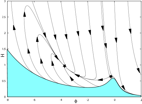
Figure 3: Typical phase portrait $(\phi,H)$, corresponding to the case $-\xi=A=\sigma=1$. Due to the symmetries of Eq. (8)-(10), the $H<0$ trajectories are obtained from the $H>0$ ones by a reflexion on $H=0$ and reversion of the arrows (time reversal operation).

suggest that it can be considerably smaller. We could verify the attractive character of the fixed point $(\bar{\phi}_{-},\bar{H}_{-})$ even for $\xi<-100$, suggesting that eventual amplifications forthcoming from the $G(\phi,\dot{\phi},H)<0$ regions are not enough to win the potential $V_{\rm eff}$ around $\bar{\phi}_{-}$. A typical phase portrait is displayed in Fig. 3, corresponding to the case $-\xi=A=\sigma=1$. The attraction basin is considerably larger than the conservative estimative base on the closed lines of constant $L$ around the fixed point. Note that all solutions starting with $\phi>\bar{\phi}_{+}$ are runaway solutions.

Figure 4: The parameter $w$ along some solutions presented in the phase portrait of Fig. 3. According to (15), solutions have $w<-1$ when $\dot{H}>0$, and $w>-1$ when $\dot{H}<0$.

Fig. 4 shows the curves $w(t)$ for some solutions presented in Fig. 3. According to (15), solutions approaching the fixed point from below have $w<-1$, while that ones doing from above have $w>-1$.

IV Conclusion

We show here that non-minimally coupled quintessential models with exponential potentials can exhibit asymptotic de Sitter phases for large sets of initial conditions. Some of these phases are characterized by a slowly evolving parameter $w=p_{\phi}/\rho_{\phi}<-1$, compatible, in principle, with the recent observational data. Our analysis is based on the existence of a Lyapunov function for the Klein-Gordon equation that can be used to estimate the attraction basin of the relevant fixed points. As it was already mentioned, real attraction basins are typically much larger than these estimations. Our results are in agreement with the linearized analysis recently proposed in faraoni .

We stress that the model presented here is free from the instabilities that are usually associated to phantom models. Classically, since $F(\phi)\neq 0$ , the model is not plagued with the anisotropic singularities described in PRD2 . Besides, since $F(\phi)$ is always positive and $V(\phi)$ is bounded from below, the model is also free from the quantum instabilities described in CHT for phantom fields.

We conclude, therefore, that it is possible, in principle, to construct realistic models for dark energy with $w<-1$. Relevant issues now are the introduction of matter fields and the study of the role played by the strong non-minimal coupling regimebartolo ; strong in the model. These points are under investigation.

- (1) A.G. Riess, et al., Astron. J. 116, 1009 (1998), astro-ph/9805201.
- (2) S. Perlmutter, et al., Astrophys. J. 517, 565 (1999), astro-ph/9812133.
- (3) P.J. Peebles and B. Ratra, Rev. Mod. Phys. 75, 559 (2003), astro-ph/0207347.
- (4) R.R. Caldwell, Rahul Dave, Paul J. Steinhardt, Phys. Rev. Lett. 80, 1582 (1998), astro-ph/9708069; L.-M. Wang, R.R. Caldwell, J.P. Ostriker, and P. J. Steinhardt, Astrophys. J. 530, 17 (2000), astro-ph/9901388.
- (5) P. J. Steinhardt, L.-M. Wang, I. Zlatev, Phys. Rev. D59, 123504 (1999), astro-ph/9812313.
- (6) J. S. Alcaniz, Phys. Rev. D69, 083521 (2004), astro-ph/0312424.
- (7) V.Faraoni, Int. J. Mod. Phys. D11, 471 (2002), astro-ph/0110067; Phys. Rev. D68, 063508 (2003).
- (8) A.G. Riess, et al., Astrophys. J. , to appear, astro-ph/0402512.
- (9) S.M. Carroll, M. Hoffman, and M. Trodden, Phys. Rev. D68, 023509 (2003), astro-ph/0301273.
- (10) S.D.H. Hsu, A. Jenkins, and M. B. Wise, Phys. Lett. B, to appear, astro-ph/0406043.
- (11) C. Rubano and P. Scudellaro, Gen. Rel. Grav. 34, 307 (2002), astro-ph/0103335; C. Rubano, et al., Phys. Rev. D69 103510 (2004), astro-ph/0311537.
- (12) J.J. Halliwell, Phys. Lett. 185B, 341 (1987); Q. Shafi and C. Wetterich, Nucl. Phys. B289, 787 (1987); I. Neupane, hep-th/0311071.
- (13) E. Gunzig, A. Saa, L. Brenig, V. Faraoni, T.M. Rocha Filho, and A. Figueiredo, Phys. Rev. D63, 067301 (2001); Int. J. Theor. Phys. 40, 2295 (2001).
- (14) L.R. Abramo, L. Brenig, E. Gunzig. and A. Saa, Phys. Rev. D67 027301 (2003); Int. J. Theor. Phys. 42 1145 (2003).
- (15) E. Gunzig and A. Saa, Int. J. Theor. Phys, to appear , gr-qc/0406068; gr-qc/0406069.
- (16) C. Baccigalupi, S. Matarrese, and F. Perrota, Phys. Rev. D62, 123510 (2000).
- (17) N. Bartolo and M. Pietroni, Phys. Rev. D61, 023518 (2000), hep-ph/9908521.
- (18) L.H. Ford and T.A. Roman, Phys. Rev. D64, 024023 (2001).
- (19) D.F. Torres, Phys. Rev. D66, 043522 (2002), astro-ph/0204504.
- (20) M. Abramowitz and I. Stegun, Handbook of Mathematical Functions, Dover, New York, (1965).
- (21) V. Faraoni, gr-qc/0407021.
- (22) V. Faraoni, Int. J. Theor. Phys. 40, 2259 (2001), hep-th/0009053; A.O. Barvinsky, Nucl. Phys. B561, 159 (1999).