Reconstructing the Primordial Spectrum with CMB Temperature and Polarization

Abstract

We develop a new method to reconstruct the power spectrum of primordial curvature perturbations, $P(k)$, by using both the temperature and polarization spectra of the cosmic microwave background (CMB). We test this method using several mock primordial spectra having non-trivial features including the one with an oscillatory component, and find that the spectrum can be reconstructed with a few percent accuracy by an iterative procedure in an ideal situation in which there is no observational error in the CMB data. In particular, although the previous “cosmic inversion” method, which used only the temperature fluctuations, suffered from large numerical errors around some specific values of $k$ that correspond to nodes in a transfer function, these errors are found to disappear almost completely in the new method.

I Introduction

The cosmic microwave background (CMB) anisotropies contain important pieces of information on physics of the early universe. The recent precise data of the Wilkinson Microwave Anisotropy Probe (WMAP) tell us that our universe is consistent with a spatially flat universe dominated by a cosmological constant ($\Lambda$) and cold dark matter (CDM), the so-called $\Lambda$CDM model, with slow-roll inflation at its early stage which has generated Gaussian, adiabatic, and nearly scale-invariant primordial fluctuations Bennett et al. (2003); Spergel et al. (2003); Peiris et al. (2003); Komatsu et al. (2003).

Nevertheless, it is reported that the observed CMB angular power spectrum may have some non-trivial features such as lack of power on large scales , running of the spectral index, and oscillatory behaviors of the spectrum on intermediate scales. To explain these non-trivial features, many authors focused on the primordial power spectrum of the curvature perturbation, $P(k)$, and proposed possible inflation models Bi et al. (2003); Contaldi et al. (2003); Cline et al. (2003); Feng and Zhang (2003); Tsujikaw et al. (2003); Kawasaki and Takahashi (2003); Piao et al. (2004); Hannestad and Mersini-Houghton (2004); Liguori et al. (2004); Kawasaki et al. (2003); Chung et al. (2003); Feng et al. (2003); Yamaguchi and Yokoyama (2003); Huang and Li (2003a, b, c); Kyae and Shafi (2003); Yamaguchi and Yokoyama (2004); Alavi and Nasseri (2004); Easther (2004); Bastero-Gil et al. (2003); Dvali and Kachru (2003); Martin and Ringeval (2004a, b, c); Kawasaki et al. (2004); Hunt and Sarkar (2004). However, equally important is to understand the implication of these observed possible non-trivial features on the primordial curvature spectrum without a theoretical prejudice. In this respect, there have been several attempts to reconstruct the primordial spectrum using the WMAP data by model-independent methods Mukherjee and Wang (2003a, b); Bridle et al. (2003); Hannestad (2004); Shafieloo and Souradeep (2003); Tocchini-Valentini et al. (2004).

In our previous work, we developed a method to reconstruct the primordial spectrum directly from the observed CMB anisotropy Matsumiya et al. (2002, 2003), which we call the cosmic inversion method, and applied it to the WMAP first-year data Kogo et al. (2004). Compared with other reconstruction methods such as the binning, wavelet band powers, and direct wavelet expansion method, we have shown that our method can reproduce fine features in $P(k)$ with a resolution of $\Delta k\simeq 3.7\times 10^{-4}\,{\rm Mpc}^{-1}$ which roughly corresponds to $\Delta\ell\simeq 5$ in the angular power spectrum, $C_{\ell}$. Performing a statistical analysis of the reconstructed $P(k)$, we have found that there are some possible deviations from scale-invariance around $k\simeq 1.5\times 10^{-2}\,{\rm Mpc}^{-1}$ and $2.6\times 10^{-2}\,{\rm Mpc}^{-1}$ Kogo et al. (2004).

The method we developed, however, used only the temperature-temperature (TT) angular power spectrum. The CMB anisotropy contains another important information, the polarization. During the recombination epoch the linear polarization of the CMB is generated by the Thomson scattering of the local quadrupole component of the temperature anisotropy Kosowsky (1996). From the perspective of a cross check, it is important to reconstruct $P(k)$ taking the CMB polarization into account. The CMB polarization was detected by the degree angular scale interferometer (DASI) for the first time Kovac et al. (2002) and more precise data of the temperature-polarization (TE) angular power spectrum were released by the WMAP recently Kogut et al. (2003). In the future, much more precise observation of the polarization will be carried out by the Planck satellite .

In this paper, we present an improved cosmic inversion method that takes account of the CMB polarization spectrum, and test our new method for various shapes of $P(k)$. That is, we calculate the CMB temperature and polarization spectra for a given $P(k)$ and reconstruct it from thus obtained CMB data. As a first step, we neglect observational errors in numerical tests and assume that the CMB temperature and polarization spectra are completely known. We calculate the CMB power spectra based on CMBFAST  but we adopt a much finer resolution than the original one in both $k$ and $\ell$. Our inversion method is an iterative method based on approximate formulas for CMB temperature and polarization spectra and correction factors that adjust the errors in the approximate formulas.

This paper is organized as follows. In Sec. II, we review the basic theory of the CMB polarization. In Sec. III, we extend our cosmic inversion method and propose a new inversion formula that uses both the CMB temperature and polarization spectra. In Sec. IV, we test our new method. We find that the primordial spectrum can be reconstructed with much better accuracy. In Sec. V, we propose the idea of constraining the cosmological parameters based on our new method. Finally, Sec. VI is devoted to conclusion.

II Basic Theory

Here we summarize basic equations for the CMB temperature fluctuations and polarization based on Zaldarriaga and Seljak (1997); Kamionkowski et al. (1997); Hu and White (1997), and their approximate formulas which are used in our inversion method. We deal only with scalar-type perturbations and assume a spatially flat universe with Gaussian and adiabatic primordial fluctuations. We leave inclusion of tensor-type perturbations for future work.

It is convenient to describe polarized radiation by the Stokes parameters Chandrasekhar (1960); Rybicki and Lightman (1960). Consider a monochromatic electromagnetic wave propagating in the $z$-direction with an angular frequency $\omega_{0}$. The components of the electric field are written as

$$E_{x} = {\cal E}_{x}(t)\cos[\omega_{0}t-\varphi_{x}(t)],$$ (1)

$$E_{y} = {\cal E}_{y}(t)\cos[\omega_{0}t-\varphi_{y}(t)].$$ (2)

The Stokes parameters are defined as

$$I \equiv \bigl{\langle}{\cal E}_{x}{}^{2}+{\cal E}_{y}{}^{2}\bigl{\rangle},$$ (3)

$$Q \equiv \bigl{\langle}{\cal E}_{x}{}^{2}-{\cal E}_{y}{}^{2}\bigl{\rangle},$$ (4)

$$U \equiv \bigl{\langle}2{\cal E}_{x}{\cal E}_{y}\cos(\varphi_{x}-\varphi_{y})\bigl{\rangle},$$ (5)

$$V \equiv \bigl{\langle}2{\cal E}_{x}{\cal E}_{y}\sin(\varphi_{x}-\varphi_{y})\bigl{\rangle},$$ (6)

where the brackets denote the time average over the modulation of the amplitudes and the phases. Since the Thomson scattering generates only linear polarization, we can neglect $V$ which describes the degree of circular polarization. Under a rotation of an angle $\psi$ on the $(x,y)$-plane, $I$ is invariant while $Q$ and $U$ are transformed as

$$Q^{\prime} = Q\cos 2\psi+U\sin 2\psi,$$ (7)

$$U^{\prime} = -Q\sin 2\psi+U\cos 2\psi,$$ (8)

which are identical to

$$(Q\pm iU)^{\prime}=e^{\mp 2i\psi}(Q\pm iU).$$ (9)

This means that $(Q\pm iU)$ have spins $\pm 2$, respectively.

We denote the temperature fluctuations and the polarization of radiation at the conformal time $\eta$ and the comoving spatial position $\bm{x}$ propagating in the direction $\hat{\bm{n}}$ as $\Theta(\eta,\bm{x},\hat{\bm{n}})$ and $(Q\pm iU)(\eta,\bm{x},\hat{\bm{n}})$, respectively. In general, these are expanded using the normal modes defined as

$${}_{s}G_{\ell m}\equiv(-i)^{\ell}\sqrt{\frac{4\pi}{2\ell+1}}\,_{s}Y_{\ell m}(\hat{\bm{n}})\,e^{i\bm{k}\cdot\bm{x}},$$ (10)

where $\bm{k}$ is the comoving wavenumber and ${}_{s}Y_{\ell m}$ is the spin-$s$ weighted spherical harmonic function Newman and Penrose (1966); Goldberg et al. (1967); Thorne (1980). For each Fourier mode we can work in the coordinate system where $\bm{k}\parallel\hat{\bm{z}}$. In the case of scalar perturbations, $m=0$,

$$\Theta(\eta,\bm{x},\hat{\bm{n}}) = \int\!\frac{d^{3}\bm{k}}{(2\pi)^{3}}\,\sum_{\ell=0}^{\infty}\Theta_{\ell}(\eta,k)\,_{0}G_{\ell 0}$$ (11)

$$= \int\!\frac{d^{3}\bm{k}}{(2\pi)^{3}}\,e^{i\bm{k}\cdot\bm{x}}\sum_{\ell=0}^{\infty}(-i)^{\ell}\Theta_{\ell}(\eta,k)P_{\ell}(\mu),$$

$$(Q\pm iU)(\eta,\bm{x},\hat{\bm{n}}) = \int\!\frac{d^{3}\bm{k}}{(2\pi)^{3}}\,\sum_{\ell=0}^{\infty}(E_{\ell}\pm iB_{\ell})(\eta,k)\,_{\pm 2}G_{\ell 0}$$ (12)

$$= \int\!\frac{d^{3}\bm{k}}{(2\pi)^{3}}\,e^{i\bm{k}\cdot\bm{x}}\sum_{\ell=0}^{\infty}(-i)^{\ell}\sqrt{\frac{(\ell-2)!}{(\ell+2)!}}\,(E_{\ell}\pm iB_{\ell})(\eta,k)P_{\ell}^{2}(\mu),$$

where $\mu\equiv\hat{\bm{k}}\cdot\hat{\bm{n}}$ and $P_{\ell}^{2}$ is the associated Legendre function, $P_{\ell}^{m}(\mu)$ with $m=2$. Here $E_{\ell}$ and $B_{\ell}$ represent the so-called E-mode and B-mode polarizations with parities $(-1)^{\ell}$ and $(-1)^{\ell+1}$, respectively. Note that for scalar-type perturbations, $B_{\ell}$ vanishes because of its parity. Using these multipole moments, the angular power spectrum is expressed as

$$\frac{2\ell+1}{4\pi}C^{X\bar{X}}_{\ell}=\frac{1}{2\pi^{2}}\int_{0}^{\infty}\!\frac{dk}{k}\,\frac{k^{3}\bigl{\langle}X_{\ell}^{*}(\eta_{0},k)\bar{X}_{\ell}(\eta_{0},k)\bigl{\rangle}}{2\ell+1},$$ (13)

where $X$ and $\bar{X}$ are either $\Theta$ ($=T$) or $E$. The Boltzmann equations for each $\Theta_{\ell}(\eta,k)$ and $E_{\ell}(\eta,k)$ can be transformed into the following integral form ($\ell\geq 2$):

$$\frac{\Theta_{\ell}(\eta_{0},k)}{2\ell+1} = \int_{0}^{\eta_{0}}\!d\eta\,\bigg{\{}\left[(\Theta_{0}+\Psi){\cal V}(\eta)+(\dot{\Psi}-\dot{\Phi})e^{-\tau(\eta)}\right]j_{\ell}(k\Delta\eta)$$ (14)

$${}+V_{b}{\cal V}(\eta)j^{\prime}_{\ell}(k\Delta\eta)+\frac{1}{2}\Pi_{2}{\cal V}(\eta)\left[3j^{\prime\prime}_{\ell}(k\Delta\eta)+j_{\ell}(k\Delta\eta)\right]\bigg{\}},$$

$$\frac{E_{\ell}(\eta_{0},k)}{2\ell+1} = -\frac{3}{2}\sqrt{\frac{(\ell+2)!}{(\ell-2)!}}\int_{0}^{\eta_{0}}\!d\eta\,\Pi_{2}{\cal V}(\eta)\,\frac{j_{\ell}(k\Delta\eta)}{(k\Delta\eta)^{2}},$$ (15)

where $\Pi_{2}\equiv(\Theta_{2}-\sqrt{6}E_{2})/10$, $\Delta\eta\equiv\eta_{0}-\eta$ with $\eta_{0}$ being the conformal time at present, and the overdot denotes a derivative with respect to the conformal time. Here $V_{b}$ is the baryon fluid velocity, $\Psi$ and $\Phi$ are the Newton potential and the spatial curvature perturbation in the Newton gauge, respectively Kodama and Sasaki (1984), and

$${\cal V}(\eta)\equiv\dot{\tau}e^{-\tau(\eta)},\quad\tau(\eta)\equiv\int_{\eta}^{\eta_{0}}\!\dot{\tau}d\eta,$$ (16)

are the visibility function and the optical depth for Thomson scattering, respectively. In the limit that the thickness of the last scattering surface (LSS) is negligible, we have ${\cal V}(\eta)\approx\delta(\eta-\eta_{*})$ and $e^{-\tau(\eta)}\approx\theta(\eta-\eta_{*})$, where $\eta_{*}$ is the recombination time when the visibility function is maximum Hu and Sugiyama (1995).

As we did in our previous papers Matsumiya et al. (2003); Kogo et al. (2004), we now take into account the thickness of the LSS approximately to perform the integrals in Eq. (15) as well as in Eq. (14) analytically. For the polarization, this is crucial since the CMB polarization is mainly generated within the thickness of the LSS. The approximation is to neglect the oscillations of the spherical Bessel functions in the integrals. Applying this approximation to Eq. (14) and (15), we have

$$\frac{\Theta_{\ell}(\eta_{0},k)}{2\ell+1} \approx \left\{\int_{\eta_{*{\rm start}}}^{\eta_{*{\rm end}}}\!d\eta\,\left[(\Theta_{0}+\Psi){\cal V}(\eta)+(\dot{\Psi}-\dot{\Phi})e^{-\tau(\eta)}\right]\right\}j_{\ell}(kd)$$ (17)

$${}+\left\{\int_{\eta_{*{\rm start}}}^{\eta_{*{\rm end}}}\!d\eta\,\Theta_{1}(\eta,k){\cal V}(\eta)\right\}j^{\prime}_{\ell}(kd)\,\,\equiv\,\,\frac{\Theta^{\rm app}_{\ell}(\eta_{0},k)}{2\ell+1},$$

$$\frac{E_{\ell}(\eta_{0},k)}{2\ell+1} \approx \sqrt{\frac{(\ell+2)!}{(\ell-2)!}}\left\{-\frac{3}{2}\int_{\eta_{*{\rm start}}}^{\eta_{*{\rm end}}}\!d\eta\,\frac{\Pi_{2}}{(k\Delta\eta)^{2}}{\cal V}(\eta)\right\}j_{\ell}(kd)\,\,\equiv\,\,\frac{E^{\rm app}_{\ell}(\eta_{0},k)}{2\ell+1},$$ (18)

where $d\equiv\eta_{0}-\eta_{*}$ is the conformal distance from the present to the LSS and $\eta_{*{\rm start}}$ and $\eta_{*{\rm end}}$ are the times when the recombination starts and ends, respectively. We have also replaced $V_{b}$ by $\Theta_{1}$ and neglected the quadrupole term in Eq. (14), by adopting the tight coupling approximation Hu and Sugiyama (1995). The transfer functions, $f(k)$, $g(k)$, and $h(k)$ are defined by

$$\int_{\eta_{*{\rm start}}}^{\eta_{*{\rm end}}}\!d\eta\,\left[(\Theta_{0}+\Psi)(\eta,k){\cal V}(\eta)+(\dot{\Psi}-\dot{\Phi})(\eta,k)e^{-\tau(\eta)}\right] \equiv f(k)\Phi(0,\bm{k}),$$ (19)

$$\int_{\eta_{*{\rm start}}}^{\eta_{*{\rm end}}}\!d\eta\,\Theta_{1}(\eta,k){\cal V}(\eta) \equiv g(k)\Phi(0,\bm{k}),$$ (20)

$$-\frac{3}{2}\int_{\eta_{*{\rm start}}}^{\eta_{*{\rm end}}}\!d\eta\,\frac{\Pi_{2}(\eta,k)}{(k(\eta_{0}-\eta))^{2}}{\cal V}(\eta) \equiv h(k)\Phi(0,\bm{k}).$$ (21)

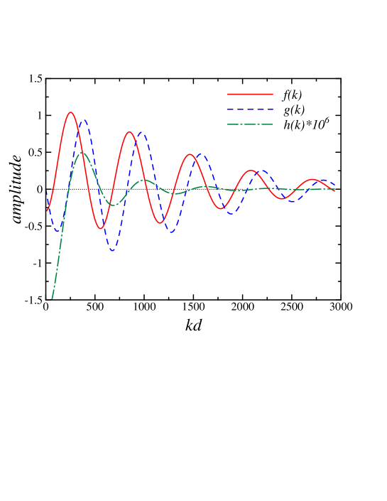
Figure 1: Transfer functions $f(k)$ (solid curve), $g(k)$ (dashed curve), and $h(k)$ (dash-dotted curve) for $h=0.70$, $\Omega_{b}=0.050$, $\Omega_{\Lambda}=0.70$, $\Omega_{m}=0.30$ and $\tau=0.20$. The horizontal axis is the comoving wavenumber normalized by $d^{-1}$, where $d\simeq 1.36\times 10^{4}\,{\rm Mpc}$ is the conformal distance from the present to the LSS. $f(k)$, $g(k)$ and $h(k)$ correspond to the monopole, dipole and quadrupole components, respectively, of the temperature anisotropy at the LSS. Since the amplitude of $h(k)$ is much smaller than those of $f(k)$ and $g(k)$, the amplitude of $h(k)$ is magnified by $10^{6}$.

Given the cosmological parameters, one can calculate transfer functions numerically, e.g., by using CMBFAST. The results are depicted in Fig. 1.

The primordial power spectrum of the curvature perturbation is defined as

$$P(k)\equiv\langle|\Phi(0,\bm{k})|^{2}\rangle.$$ (22)

Substituting Eqs. (17) and (18) into Eq. (13), we obtain the approximated TT, EE, and TE angular power spectra,

$$\frac{2\ell+1}{4\pi}C^{TT,\,{\rm app}}_{\ell} = \frac{2\ell+1}{2\pi^{2}}\int_{0}^{\infty}\!\frac{dk}{k}\,k^{3}P(k)\left[f(k)j_{\ell}(kd)+g(k)j^{\prime}_{\ell}(kd)\right]^{2},$$ (23)

$$\frac{2\ell+1}{4\pi}C^{EE,\,{\rm app}}_{\ell} = \frac{2\ell+1}{2\pi^{2}}\,\frac{(\ell+2)!}{(\ell-2)!}\,\int_{0}^{\infty}\!\frac{dk}{k}\,k^{3}P(k)\left[h(k)j_{\ell}(kd)\right]^{2},$$ (24)

$$\frac{2\ell+1}{4\pi}C^{TE,\,{\rm app}}_{\ell} = \frac{2\ell+1}{2\pi^{2}}\sqrt{\frac{(\ell+2)!}{(\ell-2)!}}\int_{0}^{\infty}\!\frac{dk}{k}\,k^{3}P(k)\left[f(k)j_{\ell}(kd)+g(k)j^{\prime}_{\ell}(kd)\right]h(k)j_{\ell}(kd).$$ (25)

III Inversion Method

Here we describe our method of the reconstruction of $P(k)$. Let us first briefly review the case of the temperature fluctuations proposed in Matsumiya et al. (2002, 2003). The CMB temperature fluctuations can be quantified by the angular correlation function defined as

$$C^{TT}(\theta)\equiv\left\langle\Theta(\hat{\bm{n}}_{1})\Theta(\hat{\bm{n}}_{2})\right\rangle=\sum_{\ell=0}^{\infty}\frac{2\ell+1}{4\pi}C^{TT}_{\ell}P_{\ell}(\cos\theta),\quad\cos\theta=\hat{\bm{n}}_{1}\cdot\hat{\bm{n}}_{2}\,.$$ (26)

Here we introduce a new variable $r$ instead of $\theta$ defined as

$$r=2d\sin\frac{\theta}{2},$$ (27)

which is the conformal distance between two points on the LSS. Substituting Eq. (23) into Eq. (26) and using the formula:

$$\sum_{\ell=0}^{\infty}(2\ell+1)P_{\ell}(\cos\theta)j_{\ell}{}^{2}(kd)=\frac{\sin kr}{kr},$$ (28)

we can derive formulas for the approximated angular correlation functions in terms of $P(k)$. In the small-scale limit $r\ll d$, its derivative is written as

$$\frac{1}{r}\frac{\partial}{\partial r}\{r^{3}C^{TT,\,{\rm app}}(r)\}=\frac{1}{2\pi^{2}}\int_{0}^{\infty}\!dk\,P(k)\left[f^{2}(k)k^{2}r\cos kr+\{2f^{2}(k)+g^{2}(k)\}k\sin kr\right].$$ (29)

Integrating by parts and applying the Fourier sine formula, we obtain a first-order differential equation for $P(k)$,

$$-k^{2}f^{2}(k)P^{\prime}(k)+\left[-2k^{2}f(k)f^{\prime}(k)+kg^{2}(k)\right]P(k)$$

$$\hskip 56.9055pt=4\pi\int_{0}^{\infty}\!dr\,\frac{1}{r}\frac{\partial}{\partial r}\{r^{3}C^{TT,\,{\rm app}}(r)\}\sin kr\equiv S^{TT}(k).$$ (30)

This is the basic equation for the inversion of the TT angular power spectrum to the primordial curvature perturbation spectrum. Note that $f(k)$ is an oscillatory function and the above differential equation is singular at $f(k)=0$. However, this can be regarded as an advantage. Namely, we can find the values of $P(k)$ at zero points of $f(k)$, say $k=k_{s}$, as

$$P(k_{s})=\frac{S^{TT}(k_{s})}{k_{s}\,g^{2}(k_{s})}\quad{\rm for}\quad f(k_{s})=0,$$ (31)

assuming that $P^{\prime}(k)$ is finite at $k=k_{s}$. Thus, without solving the differential equation, it is possible to know a rough overall feature of the spectrum. We can then solve Eq. (30) as a boundary value problem between the singularities.

Now we consider the case of the polarization. Like Eq. (26), we introduce the following quantities:

$$\tilde{C}^{EE}(\theta) \equiv \sum_{\ell=0}^{\infty}\frac{2\ell+1}{4\pi}\frac{(\ell-2)!}{(\ell+2)!}\,C^{EE}_{\ell}P_{\ell}(\cos\theta),$$ (32)

$$\tilde{C}^{TE}(\theta) \equiv \sum_{\ell=0}^{\infty}\frac{2\ell+1}{4\pi}\sqrt{\frac{(\ell-2)!}{(\ell+2)!}}\,C^{TE}_{\ell}P_{\ell}(\cos\theta).$$ (33)

These are defined in such a way that the factors $(\ell+2)!/(\ell-2)!$ and $\sqrt{(\ell+2)!/(\ell-2)!}$ in $C^{EE}_{\ell}$ and $C^{TE}_{\ell}$, respectively, are canceled out so that we can use the formula (28). Note that they are not the conventional angular correlation functions but just quantities that are convenient for inversion. Substituting Eqs. (24) and (25) into Eqs. (32) and (33), respectively, in the small-scale limit $r\ll d$, we have

$$r\tilde{C}^{EE,\,{\rm app}}(r) = \frac{1}{2\pi^{2}}\int_{0}^{\infty}\!dk\,kh^{2}(k)P(k)\sin kr,$$ (34)

$$r\tilde{C}^{TE,\,{\rm app}}(r) = \frac{1}{2\pi^{2}}\int_{0}^{\infty}\!dk\,kf(k)h(k)P(k)\sin kr\,.$$ (35)

We obtain expressions much simpler than that for the TT case. Applying the Fourier sine formula, we obtain the algebraic equations for $P(k)$,

$$kh^{2}(k)P(k) = 4\pi\int_{0}^{\infty}\!dr\,r\tilde{C}^{EE,\,{\rm app}}(r)\sin kr\equiv S^{EE}(k),$$ (36)

$$kf(k)h(k)P(k) = 4\pi\int_{0}^{\infty}\!dr\,r\tilde{C}^{TE,\,{\rm app}}(r)\sin kr\equiv S^{TE}(k).$$ (37)

In this case, we can find $P(k)$ at the values of $k$ where $h(k)\neq 0$ for EE, and at those where $f(k)\neq 0$ and $h(k)\neq 0$ for TE without solving a differential equation. The equations (36) and (37) are the basic inversion formulas for the EE and TE angular power spectra, respectively.

In practice, however, we find that numerical errors become large around the singularities of Eq. (36) or (37), where the prefactor of $P(k)$ vanishes, if we use either of them for inversion. We encountered a similar numerical problem in the TT case when we used Eq. (30) for inversion, particularly when observational errors in the CMB power spectrum were taken into account Kogo et al. (2004). Here, as a remedy for this numerical problem, we propose a new method that combines the TT and EE formulas. Since the zero points of $f(k)$ and $h(k)$ are different from each other as shown in Fig. 1, we expect this to suppress numerical errors around the zero points of both $f(k)$ and $h(k)$.

Multiplying Eq. (36) by some factor $\alpha$ (which we take to be independent of $k$ for simplicity), and adding it to Eq. (30), we obtain the combined inversion formula as

$$-k^{2}f^{2}(k)P^{\prime}(k)+\left[-2k^{2}f(k)f^{\prime}(k)+kg^{2}(k)+\alpha kh^{2}(k)\right]P(k)=S^{TT}(k)+\alpha S^{EE}(k),$$ (38)

and the boundary conditions are similarly given by the values of $P(k)$ at zero points of $f(k)$ as

$$P(k_{s})=\frac{S^{TT}(k_{s})+\alpha S^{EE}(k_{s})}{k_{s}\left[g^{2}(k_{s})+\alpha h^{2}(k_{s})\right]}\quad{\rm for}\quad f(k_{s})=0,$$ (39)

assuming that $P^{\prime}(k)$ is finite at $k=k_{s}$. The contribution of EE is controlled by the parameter $\alpha$. If we take an appropriate value of $\alpha$ so that the contribution of EE is comparable to that of TT, the solution of Eq. (38) becomes numerically stable even around the singularities because the contribution of EE dominates near the singularities of TT given by $f(k)=0$, and vice versa. We investigate this in the next section.

We do not use the TE formula, Eq. (37), because it is singular not only at $h(k)=0$ but also at $f(k)=0$ where the TT formula is also singular . Perhaps the TE spectrum can be used as a consistency check when we have accurate temperature and polarization maps at hand. However, here we do not discuss it.

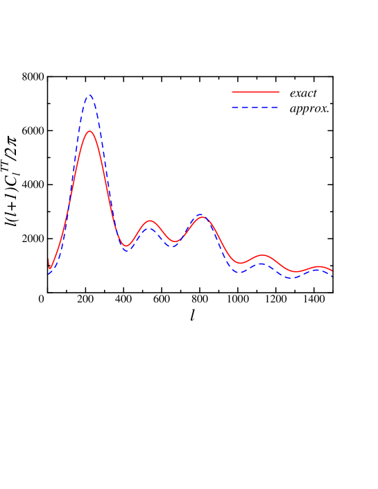
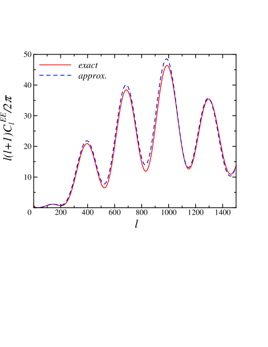
Figure 2: Comparison of the exact spectrum $C^{XX,\,{\rm ex}}_{\ell}$ (solid curves) with the approximated one $C^{XX,\,{\rm app}}_{\ell}$ (dashed curves) for TT (top panel) and EE (bottom panel). The cosmological parameters are the same as those in Fig. 1, and $P(k)$ is assumed to be scale invariant. The relative errors of $C^{XX,\,{\rm app}}_{\ell}$ are as large as $20-30\%$ for both TT and EE.

For either TT or EE, the approximated spectrum $C^{XX,\,{\rm app}}_{\ell}$ ($X=T$ or $E$) used to obtain the inversion formula has relative errors as large as about $20-30\%$ when compared with the exact one $C^{XX,\,{\rm ex}}_{\ell}$. We show $C^{XX,\,{\rm ex}}_{\ell}$ and $C^{XX,\,{\rm app}}_{\ell}$ for TT and EE in Fig. 2. Of course, since the observed spectrum $C^{XX,\,{\rm obs}}_{\ell}$ is to be compared with $C^{XX,\,{\rm ex}}_{\ell}$, it is necessary to correct the errors. For this purpose, we first define the ratio,

$$b^{XX}_{\ell}\equiv\frac{C^{XX,\,{\rm ex}}_{\ell}}{C^{XX,\,{\rm app}}_{\ell}}\,.$$ (40)

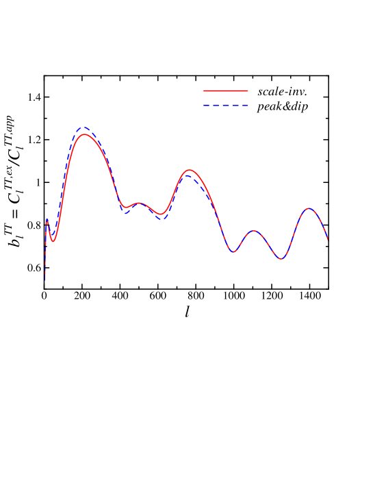
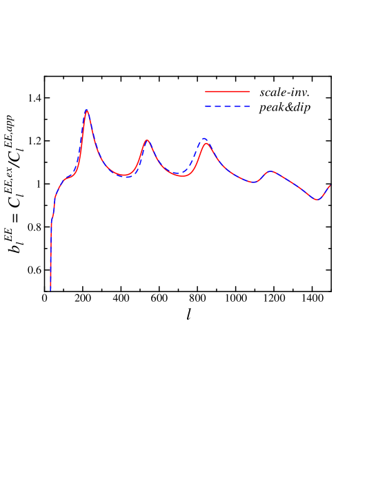
Figure 3: Comparison of $b^{XX}_{\ell}$ between the case of a scale-invariant $P(k)$ (solid curves), and that of $P(k)$ with a peak and a dip (dashed curves), for TT (top panel) and EE (bottom panel). The cosmological parameters are the same as those in Fig. 1. The relative differences of $b^{XX}_{\ell}$ between these two cases are about $5\%$ for both TT and EE, implying the weak dependence of $b^{XX}_{\ell}$ on $P(k)$.

Interestingly, this ratio is found to be almost independent of $P(k)$ not only for TT Matsumiya et al. (2003) but also EE. Figure 3 shows $b^{TT}_{\ell}$ and $b^{EE}_{\ell}$ for a scale-invariant $P(k)$ and a spectrum with a peak and a dip. In this case, the difference is found to be less than about $5\%$. We use this property of $b^{XX}_{\ell}$ to perform an iteration of inversion as previously done in the TT case Matsumiya et al. (2002, 2003).

For self-containedness, let us recapitulate the iterative procedure. First we calculate $b^{XX,\,(0)}_{\ell}=C^{XX,\,{\rm ex}(0)}_{\ell}/C^{XX,\,{\rm app}(0)}_{\ell}$, for a fiducial primordial spectrum $P^{(0)}(k)$ such as a scale-invariant one. Then we divide the observed spectrum $C^{XX,\,{\rm obs}}_{\ell}$ by $b^{XX,\,(0)}_{\ell}$; $C^{XX,\,{\rm obs}}_{\ell}/b^{XX,\,(0)}_{\ell}$. This gives a better guess to $C^{XX,\,{\rm app}}_{\ell}$. We use it to evaluate $S^{XX}(k)$ in the right-hand side of Eq. (38) and solve this equation. Let us denote the reconstructed primordial spectrum from $C^{XX,\,{\rm obs}}_{\ell}/b^{XX,\,(0)}_{\ell}$ by $P^{(1)}(k)$. Then we can repeat the same procedure and obtain $P^{(2)}(k)$ from $C^{XX,\,{\rm obs}}_{\ell}/b^{XX,\,(1)}_{\ell}$, where $b^{XX,\,(1)}_{\ell}$ is calculated from $P^{(1)}(k)$. Repeating this procedure as many times as it is necessary, we can find $P(k)$ with much better accuracy. The $n$-th iteration is summarized as

$$\cdots\Rightarrow\,\,P^{(n-1)}(k)\,\,\rightarrow\,\,b_{\ell}^{XX,\,(n-1)}=\frac{C^{XX,\,{\rm ex}(n-1)}_{\ell}}{C^{XX,\,{\rm app}(n-1)}_{\ell}}\,\,\rightarrow\,\,\frac{C^{XX,\,{\rm obs}}_{\ell}}{b_{\ell}^{XX,\,(n-1)}}\,\,\Rightarrow\,\,P^{(n)}(k)\,\,\rightarrow\cdots.$$ (41)

We confirm that this iteration converges within a few times as discussed in the next section.

IV Numerical Tests

To test our inversion method including the CMB polarization, we perform the reconstruction of $P(k)$ from $C^{XX}_{\ell}$ for several $P(k)$ whose shapes are given by hand. As mentioned before, we assume here an ideal situation in which the CMB data contain no observational error. We use $C^{XX}_{\ell}$ up to $\ell_{\rm max}=1500$ for both TT and EE. As a fiducial spectrum, $P^{(0)}(k)$, for the iteration, we choose a scale-invariant spectrum $k^{3}P(k)=\mbox{const.}$, and assume the cosmological parameters as $h=0.70$, $\Omega_{b}=0.050$, $\Omega_{\Lambda}=0.70$, $\Omega_{m}=0.30$, and $\tau=0.20$. In this case, the positions of the singularities for $f(k)=0$ are at $kd\simeq 70$, $430$, $680$, $1030$, $\cdots$, and for $h(k)=0$ are at $kd\simeq 230$, $560$, $860$, $1180$, $\cdots$, where $d\simeq 1.36\times 10^{4}\,{\rm Mpc}$. We solve Eq. (38) as a boundary value problem between the first and fourth TT singularities for $f(k)=0$. Hence the range of the reconstructed $P(k)$ is $70\leq kd\leq 1030$, where $kd$ roughly corresponds to $\ell$. When proceeding from the $(n-1)$-th to $n$-th iteration, we need $P^{(n-1)}(k)$ up to $k_{\rm max}d\simeq 2\ell_{\rm max}$ to calculate $b^{XX,\,(n-1)}_{\ell}$. Hence we assume the scale-invariance outside of the reconstructed range.

First we examine the dependence of the reconstructed $P(k)$ on the parameter $\alpha$ appeared in Eq. (38), which controls the contribution of EE, assuming that the cosmological parameters are known. We assume that $P(k)$ has a peak and a dip expressed as

$$k^{3}P(k)=A\left\{1+a_{1}\exp\left[-\frac{(k-k_{1})^{2}}{\sigma_{1}{}^{2}}\right]\right\}\left\{1+a_{2}\exp\left[-\frac{(k-k_{2})^{2}}{\sigma_{2}{}^{2}}\right]\right\}^{-1},$$ (42)

and we take $a_{1}=a_{2}=1.0$, $k_{1}=0.03\,{\rm Mpc}^{-1}$, $k_{2}=0.06\,{\rm Mpc}^{-1}$, $\sigma_{1}=0.01\,{\rm Mpc}^{-1}$, and $\sigma_{2}=0.005\,{\rm Mpc}^{-1}$. Figure 4 depicts the reconstructed $P(k)$ with four different values of $\alpha$. The case $\alpha=0$ corresponds to the result of the original cosmic inversion method. We show only $P^{(1)}(k)$ for each $\alpha$, which means that no iteration is performed, to see the effect of the contribution of EE explicitly. We find that the reconstructed $P(k)$ is in a good agreement with the original one even near the singularities for $\alpha=10^{15}$, while spurious sharp features appear near the TT singularities for $\alpha$ much smaller than $10^{15}$ and those appear near the EE singularities for $\alpha$ much larger than $10^{15}$. This behavior is reasonable because the contribution of EE is found to be of the same order of TT for $\alpha\sim 10^{14-15}$ by comparing their magnitudes in the source terms of Eq. (38). Therefore, we adopt $\alpha=10^{15}$ in the following reconstructions. It may be noted that the origin of this number, $\sim 10^{14-15}$, comes dominantly from the fact that the transfer function $h(k)$ for EE is intrinsically smaller than the transfer functions $f(k)$ and $g(k)$ for TT by a factor $\sim 10^{-7}$ (see Fig. 1) and their squares are contained in the left-hand side of Eq. (38).

We perform the inversion for several shapes of $P(k)$, assuming that the cosmological parameters are known.

• Spectrum with a peak and a dip

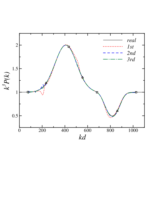
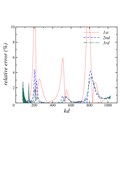
Figure 5: Reconstructed spectrum for $P(k)$ with a peak and a dip, given by Eq. (42) in the text. The top panel shows the results after each round of iteration, and the bottom panel shows their relative errors, $|P^{(n)}(k)-P^{\rm real}(k)|/P^{\rm real}(k)$. The singularities $f(k)=0$ are denoted by $\square$, and $h(k)=0$ by $\triangle$.

  Figure 5 shows the results of the iteration for $P(k)$ given by Eq. (42). We see that the iteration converges within a few times and the relative errors are reduced to about a few percent level. In Matsumiya et al. (2003), it has been shown that in the case of using the TT spectrum only, which is identical to $\alpha=0$ here, one can reconstruct $P(k)$ with about a few percent errors by iteration, cutting off spurious sharp features appeared near the singularities and interpolating the spectrum smoothly at each step of iteration. But with our new method, it became unnecessary to perform this artificial modification of the spectrum during iteration.

• Spectrum with a running spectral index

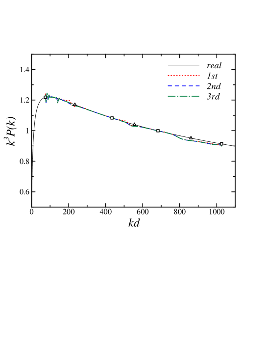
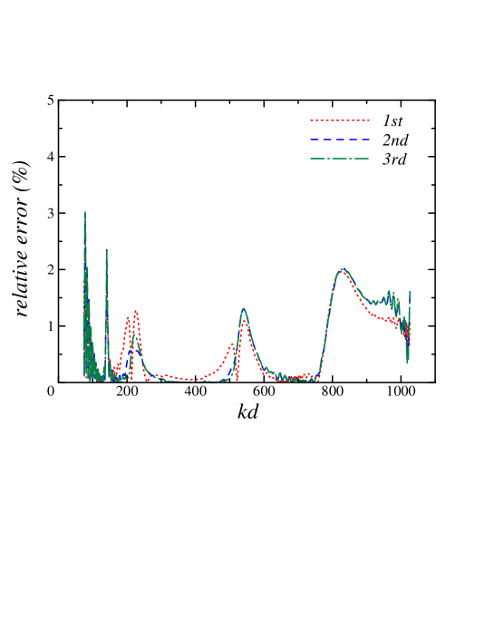
Figure 6: The same as Fig. 5, but for $P(k)$ with a running spectral index, given by Eq. (43) in the text. In this case, the errors are already less than $3\%$ at the first round of iteration, and they remain stably at that level after the second and third rounds of iteration.

  Figure 6 shows the results for $P(k)$ with a running spectral index given by Kosowsky and Turner (1995)

  $$k^{3}P(k)=A\left(\frac{k}{k_{0}}\right)^{n(k)-1},\quad n(k)=n(k_{0})+\frac{dn}{d\ln k}\ln\left(\frac{k}{k_{0}}\right).$$ (43)

  We take $k_{0}=0.05\,{\rm Mpc}^{-1}$, $n(k_{0})=0.8$, and $dn/d\ln k=-0.05$.

• Spectrum with an oscillatory component

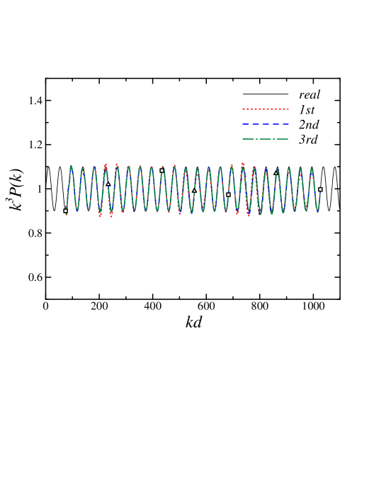
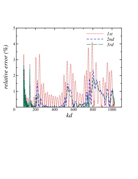
Figure 7: The same as Fig. 5, but for $P(k)$ with an oscillatory component, given by Eq. (44) in the text. The results are quite impressive because such a small oscillation like this can be reconstructed with the errors less than $3\%$.

  Figure 7 shows the results for $P(k)$ with an oscillatory component given by

  $$k^{3}P(k)=A\left[1+a_{0}\sin\left(\frac{k}{k_{0}}\right)\right].$$ (44)

  This form is motivated by possible signatures of trans-Planckian physics Martin and Brandenberger (2001); Brandenberger and Martin (2001); Martin and Brandenberger (2003). We take $a=0.1$ and $k_{0}=5\times 10^{-4}\,{\rm Mpc}^{-1}$.

The results are quite impressive because we can reconstruct not only a global shape such as a running spectral index, but also a fine feature such as a small oscillation as given by Eq. (44) with only a few percent errors.

V Novel Method to Constrain Cosmological Parameters

We also examine how the shape of reconstructed $P(k)$ changes if we adopt the values of the cosmological parameters different from the assumed values, namely, those used in making a mock sample of $C^{XX}_{\ell}$. We vary each cosmological parameter in the range of about $2\sigma$ of its current best-fit value, that is, $0.60\leq h\leq 0.80$, $0.040\leq\Omega_{b}\leq 0.060$, and $0.60\leq\Omega_{\Lambda}\leq 0.80$, respectively, with the others fixed in the case of a scale-invariant $P(k)$. We do not vary $\tau$ since it affects only the normalization except for the spectrum on large scales.

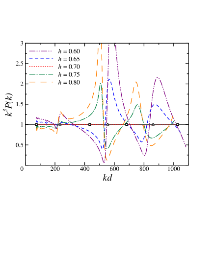
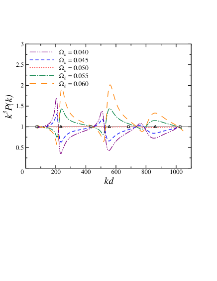
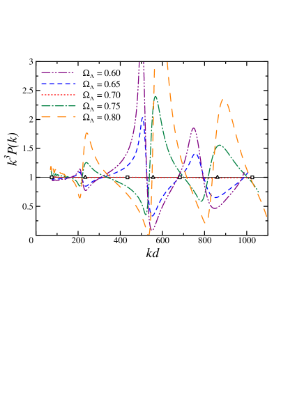
Figure 8: Dependence of the reconstructed $P(k)$ on the cosmological parameters different from the presumed real values. We assume a scale-invariant $P(k)$ and the cosmological parameters as $h=0.70$, $\Omega_{b}=0.050$, $\Omega_{\Lambda}=0.70$, $\Omega_{m}=0.30$, and $\tau=0.20$. The top left panel shows the reconstruction by varying $h$ over $h=0.60$, $0.65$, $0.70$, $0.75$, and $0.80$. The top right panel shows the reconstruction by varying $\Omega_{b}$ over $\Omega_{b}=0.040$, $0.045$, $0.050$, $0.055$, and $0.060$. The bottom panel shows the reconstruction by varying $\Omega_{\Lambda}$ over $\Omega_{\Lambda}=0.60$, $0.65$, $0.70$, $0.75$, and $0.80$. In all the cases, the other parameters are fixed at the presumed values. Note that the value of $d$ and the positions of the singularities depend on the cosmological parameters. Plotted are the singularities ($f(k)=0$ by $\square$ and $h(k)=0$ by $\triangle$) in the case of the presumed values of the cosmological parameters.

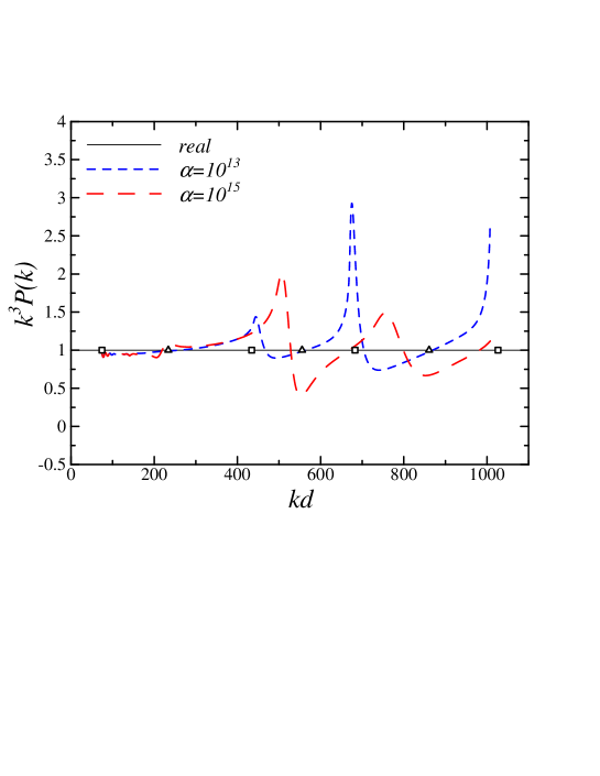
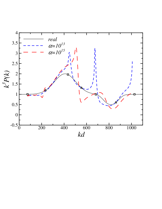
Figure 9: Dependence of the reconstructed $P(k)$ on the parameter $\alpha$ in the case that one of the cosmological parameters is incorrect. Assumed values of the cosmological parameters are the same as those in Fig. 8. Both are the cases that we use an incorrect value, $h=0.75$ in our reconstruction for $\alpha=10^{13}$ and $10^{15}$. The top panel shows the reconstructed spectra for a scale-invariant $P(k)$ and the bottom panel shows those for $P(k)$ with a peak and a dip given by Eq. (42) in the text. Plotted are the singularities in the same way as Fig. 8.

The resultant $P^{(1)}(k)$ are shown in Fig. 8. We see that if we use incorrect values of the cosmological parameters in our reconstruction procedure, the reconstructed $P(k)$ is deformed from its real shape near the EE singularities for $\alpha=10^{15}$. This is because the contribution of EE is slightly larger than that of TT. If we adopt a smaller value of $\alpha$ so that the contribution of TT is larger than that of EE, such a deformation appears near the TT singularities. In fact, this was the case studied in Matsumiya et al. (2003) which corresponds to the extreme case $\alpha=0$ using only the TT spectrum. Figure 9 shows how the reconstructed $P(k)$ with incorrect values of the cosmological parameters changes depending on $\alpha$ for the case that $P(k)$ is scale invariant and that it has a peak and a dip given by Eq. (42).

In the previous case where we use only TT spectrum, even if we ended up with a spiky shape of the reconstructed $P(k)$ around some specific values of $k$, it is difficult to judge if it was a real feature or simply an artifact due to the incorrect choice of the cosmological parameters. In contrast, in the present case where we use both TT and EE spectra, we can invent a new method to constrain the cosmological parameters without assuming the shape of $P(k)$ from the following two observations. First, as shown in Fig. 4, in the range of $10^{13}\lesssim\alpha\lesssim 10^{15}$, $P(k)$ is reconstructed rather well if we use the correct values of the cosmological parameters. On the other hand, if we use incorrect values in our reconstruction, we obtain a deformed shape of the reconstructed $P(k)$. Now, as shown in Fig. 9, the location of the deformation in $k$-space depends on the value of $\alpha$ we use. That is, if we take a relatively large value of $\alpha$, say, $\alpha_{1}\sim 10^{15}$, the deformation is most prominent around the EE singularities. On the other hand, if we use a smaller value, say, $\alpha_{2}\sim 10^{13}$, the location of the deformation moves to the TT singularities. Thus unless we adopt the cosmological parameters which are close enough to the real values, the shape of $P_{\alpha_{1}}(k)$, namely the reconstructed spectrum for $\alpha=\alpha_{1}$, will be much different from the shape of $P_{\alpha_{2}}(k)$, that for $\alpha=\alpha_{2}$. Thus we may obtain constraints on the cosmological parameters by comparison of the shapes of $P_{\alpha_{1}}(k)$ and $P_{\alpha_{2}}(k)$. An intriguing point is that no assumption on the shape of $P(k)$ is necessary to derive the constraints.

VI Conclusion

We have derived the inversion formula including both the CMB temperature fluctuations and polarization, and examined the validity of our inversion method. Our method is based on a linear combination of inversion formulas for approximate temperature (TT) and polarization (EE) spectra in the form $\mbox{TT}+\alpha\mbox{EE}$, given by Eq. (38), with a constant parameter $\alpha$, combined with iteration that corrects errors in the approximate formulas.

First we have examined the effect of the contribution of EE on the reconstructed $P(k)$. There are singularities in the TT and EE inversion formulas due to the zero points of transfer functions. We have found that large numerical errors in the reconstructed $P(k)$ around the singularities of the TT and EE inversion formulas, which appear when each formula is used independently, disappear for the choice of $\alpha\sim 10^{14-15}$, for which the contribution of EE becomes comparable to that of TT. Using such an appropriate value of $\alpha$, we have tested our method against several presumed spectral shapes of $P(k)$. As a result, we have confirmed that the relative errors between the reconstructed $P(k)$ and the original one are reduced to a few percent level after a few steps of iteration.

We have also examined the case when the cosmological parameters are varied from the presumed real values. For the choice of $\alpha=10^{15}$, we have shown that the reconstructed $P(k)$ is substantially deformed from its real shape near the EE singularities, while it is substantially deformed near the TT singularities for much smaller values of $\alpha$. Since the errors near the singularities in the reconstructed $P(k)$ are relatively small for any $\alpha$ in the range of $10^{13}\lesssim\alpha\lesssim 10^{15}$, if the correct cosmological parameters are chosen, this result suggests a new method for constraining the cosmological parameters. Namely, by comparison of reconstructed $P(k)$ for different values of $\alpha$, we may constrain the cosmological parameters without any assumption on the shape of $P(k)$.

In this paper, we have not taken account of possible observational errors. In reality, of course, observational errors are by no means negligible. As shown in Kogo et al. (2004), in the case of using the TT spectrum of the WMAP, numerical errors are enhanced near the singularities, which made us impossible to obtain any information of $P(k)$ near the singularities. However, our new method that substantially suppresses the numerical errors around the singularities may not suffer much from this difficulty. In any case, it is important to investigate the effect of observational errors on our new method. It is also important to investigate the possibility of using our new inversion method to constrain the cosmological parameters by taking account of observational errors. Since we will inevitably obtain different shapes of $P(k)$ for different choices of $\alpha$ under the presence of observational errors, even if we knew and used the true cosmological parameters, it is necessary to develop a statistical criterion that tests the equivalence of the shapes of reconstructed $P(k)$. It is also necessary to extend our method to include the contribution of tensor-type perturbations, which is probed by the B-mode polarization. Their contribution may be appreciable as predicted in many models of inflation Starobinsky (1979); Rubakov et al. (1982); Abbott and Wise (1984); Polnarev (1985); Crittenden et al. (1993a, b). These issues will be investigated in the future.

Figure 4: Dependence of the reconstructed $P(k)$ on the parameter $\alpha$ which controls the contribution of EE relative to TT, for the presumed form of $P(k)$ given by Eq. (42) in the text. The cosmological parameters are assumed to be known. The result of reconstruction is shown for $\alpha=0$, $10^{13}$, $10^{15}$, and $10^{17}$. The horizontal axis $kd$ roughly corresponds to $\ell$. The singularities $f(k)=0$ are denoted by $\square$, and $h(k)=0$ by $\triangle$. In the case of $\alpha=10^{15}$, for which the contributions of TT and EE are comparable, the errors are substantially suppressed, especially near the singularities.