Sunyaev-Zel’dovich polarization simulation

Abstract

Compton scattering of Cosmic Microwave Background (CMB) photons on galaxy cluster electrons produces a linear polarization, which contains some information on the local quadrupole at the cluster location. We use N-body simulations to create, for the first time, maps of this polarization signal. We then look at the different properties of the polarization with respect to the cluster position and redshift.

,

1 Introduction

Photons from the last scattering surface (the cosmic microwave background; CMB) propagate toward us, interacting with the matter in between. These interactions cause a change in the temperature and polarization pattern of the CMB. For instance, Compton scattering can produce linear polarization if the interacting medium is illuminated by a quadrupolar radiation field.
Sunyaev & Zel’dovich (1980) first explored the different effects on CMB polarization that galaxy clusters, here the interacting medium, could produce and distinguished 3 sources : the primordial CMB quadrupole seen by the clusters, the quadrupole produced by a first interaction inside the cluster, and the transverse velocity of the cluster. Similar effects have been proposed more recently (Chluba & Mannheim, 2002; Diego et al., 2003). Though these are very small signals, it has been advocated that one can get interesting information on the CMB quadrupole (Kamionkowski & Loeb, 1997; Portsmouth, 2004) and the cluster transverse velocity (Sunyaev & Zel’dovich, 1980; Sazonov & Sunyaev, 1999; Audit & Simmons, 1999) through these effects. Cooray & Baumann (2003) have shown that the contribution from the primordial quadrupole dominates the signal, it will therefore be the focus of our work.
In this paper we present the first map of the polarization arising from the primordial quadrupolar CMB anisotropies (though see Delabrouille et al. (2002) and Melin (2004) for simulations of other SZ effects) and look for the typical properties of the signal. We describe in the following our physical model of the induced polarization, we then show how we simulate the effect under reasonable assumptions, we finish by showing interesting properties of this simulation.

2 Model

The primordial CMB quadrupole is generated by two effects : the SW (Sachs-Wolfe) effect and the ISW (Integrated SW) effect which for adiabatic fluctuations in the cluster reference frame can be written as (Sachs & Wolfe, 1967) :

$$\hskip 85.35826pt\frac{\Delta T_{\mathrm{SW}}(\hat{n})}{T} = -{1\over 3}\;{\Phi(\hat{n},z_{\rm CMB})}$$ (1)

$$\hskip 85.35826pt\frac{\Delta T_{\mathrm{ISW}}(\hat{n})}{T} = -2\int_{z_{\rm CMB}}^{z_{\rm clus}}\dot{\Phi}({\hat{n}},z)dz$$ (2)

where $z_{\rm clus}$ is the cluster redshift, $z_{\rm CMB}\simeq 10^{3}$ is the redshift of the last scattering surface, and $\hat{n}$ is the angular position of the cluster. The cross section for Compton scattering is :

$$\frac{d\sigma}{d\Omega}=\frac{3\sigma_{T}}{8\pi}|{\hat{\epsilon}}_{\rm in}\cdot{\hat{\epsilon}}_{\rm out}|^{2}$$ (3)

where ${\hat{\epsilon}}_{\rm in}$, ${\hat{\epsilon}}_{\rm out}$ stand respectively for the input and output photon polarization vector, and $\sigma_{T}$ for the Thomson cross-section. Using the stokes parameters Q and U, defining our coordinate system (centered on the cluster) with the axis $\hat{z}$ in the line of sight direction ($x$ and $y$ axis will define $Q$ and $U$ basis), and integrating on all incoming photon directions, we get :

$$\hskip 85.35826ptQ\,({\hat{z}}) = \frac{3\sigma_{T}}{16\pi}\int{\Delta T(\hat{n})\sin^{2}\theta\cos 2\phi d\Omega}$$ (4)

$$\hskip 85.35826ptU\,({\hat{z}}) = \frac{3\sigma_{T}}{16\pi}\int{\Delta T(\hat{n})\sin^{2}\theta\sin 2\phi d\Omega}$$ (5)

Substituting $\Delta T_{\mathrm{SW}}(\hat{n})+\Delta T_{\mathrm{ISW}}(\hat{n})$ for $\Delta T(\hat{n})$ and $\tau_{\rm clus}$ for $\sigma_{T}$ in the above, we obtain the polarization created by clusters for a given potential $\Phi$.

3 Simulations

In order to create a $\Phi$ field with which we compute the local quadrupole, we generated a cube of $256^{3}$ points covering 30 Gpc in size at $z=0$, which gave us enough space to trace back to the last scattering surface ($z\simeq 1100$) with sufficient resolution (around 100 Mpc/h) to compute the integrals in §2.
We used a simple Harrison-Zel’dovich, or scale-invariant, spectrum to model the potential fluctuations as we only look at very large scales. We then used an N-body simulation (see Vale et al. (2004); Amblard et al. (2004) for more details) to compute $\tau_{\rm clus}$ in different $z$ slices (35 from z = 0 to 2). The last step is to combine all of these ingredients :

$$Q(\hat{u})= -\sum_{i}\frac{3\tau_{\rm clus}(z_{i})}{16\pi}\sum_{\theta,\phi}\left\{{\Phi(r_{i}\hat{u}+r^{\scriptscriptstyle{\rm CMB}}_{i}\hat{n},z_{\rm\scriptscriptstyle{CMB}})\over 3}+2\sum_{j}\dot{\Phi}(r_{i}\hat{u}+r_{j}\hat{n},z_{j})\right\}$$ (6)

$$\times\sin^{2}\theta\cos 2\phi\Delta z\Delta\Omega$$

$\tau_{\rm clus}(z_{i})$ stands for the optical depth at redshift $z_{i}$ (corresponding to one of our N-body simulation slices), $r_{i}$ represents the distance to this redshift, $\hat{n}$ is the unit vector of direction $(\theta,\phi)$ (we map the directions using the HEALPix package), and $r_{i}^{\rm CMB}$ is the distance to the last scattering surface from the redshift $z_{i}$. We obtain $U(\hat{u})$ by substituting $\cos 2\phi$ by $\sin 2\phi$.
From these Q and U maps we can compute the polarization fraction and angle or the E and B maps. In order to keep our algorithm simple and fast we do not use any interpolation on our $256^{3}$ map, but we test by changing the resolution of the different quantities that our accuracy is better than 10%. We note that our result includes only contributions to the signal from clusters with $z<2$. Though these clusters are the dominant signal for our purposes, source at higher redshift may contribute significantly to the signal on large scales.

4 Results

Our basic result is shown in Figure 1, which displays the polarization pattern expected over a 7.5^∘ patch of the sky. The polarization amplitude goes up to 0.16 $\mu$K, the maximum amplitude depends of the cluster position (here maximum around $(l,b)\simeq(40,60)$ or $(-40,240)$, see figure 4) and redshift (here maximum achieved around $z\simeq 1.6$, see figure 5) with respect to the value of the quadrupole.

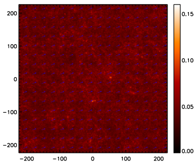
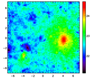
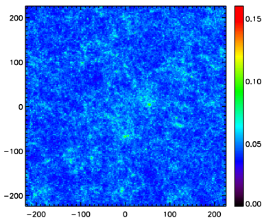
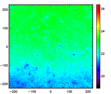
Figure 1: Top Left : Polarization pattern of 7.5$\times$7.5 degrees (axis scales in arcminutes) patch located around (0,0) : the color scale (maximum set to 0.16 $\mu$K in order to reveal more structures) indicates the polarization amplitude $P=\sqrt{Q^{2}+U^{2}}$, arrows indicate the polarization angle. Top Right : Polarization angle (in degrees) for the area around (2,-67) on the left plot, this area contains 2 massive clusters of 1.15$\times 10^{15}\mathrm{M}_{\odot}$ (red spot on the right) and 6.25$\times 10^{14}\mathrm{M}_{\odot}$ (blue spot on the left) at a respective redshift of 0.25 and 1.11. Bottom : polarization amplitude (left) and angle (right in degrees) of our 7.5^∘ patch, notice the 2 effects on the polarization angle pattern, one due to the alignment with the quadrupole (large scale gradient), and one due to the different redshift values of the clusters (small scales).

Our particular realization does not maximize the polarized signal coming from the SZ, but gives a reasonable estimate of its amplitude which in any case would not exceed a few tenths of 1$\mu$K. The signal for polarized Sunyaev-Zel’dovich effect is therefore not detectable with present technology (eq. B2K2 and Maxipol should achieved around 50 $\mu$K/arcmin) on any scales. Future surveys (Polarbear II, CMBPol), which should achieve a sensitivity around 1$\mu$K/arcmin, may have enough sensitivity to measure the effect on the larger scales ($\ell<200$). On the figure 2, we compared the polarized CMB lensing effect with the polarized SZ by showing a patch of our simulated sky around the 2 massive clusters in figure 1 (red spot on the right and blue spot on the left with a respective mass of 1.15$\times 10^{15}\mathrm{M}_{\odot}$ and 6.25$\times 10^{14}\mathrm{M}_{\odot}$ and a respective redshift of 0.25 and 1.11). The B mode amplitude from the polarized SZ is around 0.1 $\mu$K, much lower than the one coming from the CMB lensing (around 3$\mu$K). Therefore even if the sensitivity to detect the polarized SZ could be achieved one would have to disentangle it from the CMB lensing signal. The very different pattern of the two B mode signals (CMB lensing is much smoother and correlated to the E mode gradient) could maybe help in such a task.

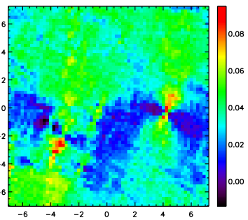
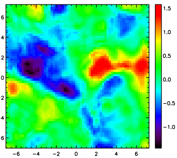
Figure 2: Part of the 7.5$\times$7.5 degree map centered around 2 massive clusters (same area as Figure 1 top right). The left map represents the polarized SZ B mode, the right map the contribution of the lensing to the B mode. The amplitutde of the polarized SZ ($\simeq 0.1\mu\mathrm{K}$) is about 30 times smaller than the lensing of the CMB ($\simeq 3\mu\mathrm{K}$).

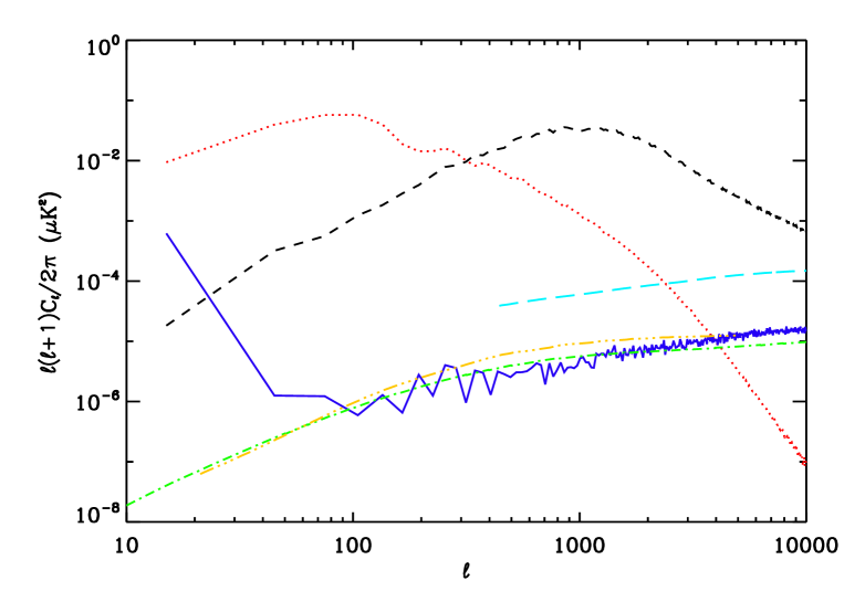
Figure 3: The B mode power spectra of the primordial CMB with tensor/scalar ratio of 1 (red dots), lensed CMB (black dashes) and Sunyaev Zel’dovich effect (blue solid line). Previous estimate from Cooray et al. (2004) (green dot dashed line), Hu (2000) (orange dash-triple dotted line) and recent estimate from Liu et al. (2005) (light blue long dashed line) are also shown for comparison. The SZ power spectrum can be subdivided in two parts : on large scale ($\ell<40$) the geometrical projection effect of the quadrupole dominates, on small scale ($\ell>100$) the variation of the optical depth dominates.

From the different maps (polarized SZ, primordial CMB, lensing of the CMB), we compute the power spectra (see figure 3). The B mode of the polarized SZ is very small relative to the lensing of the CMB and to the primordial CMB (here we took an “optimistic” tensor to scalar ratio of unity, $r=1$) from $\ell=20$ to $10000$. Only the B mode spectra are shown on figure 3 but the E mode spectrum of the polarized SZ is identical to the B mode ones, so that polarized SZ E mode are even more subdominant compared to other sources. Our estimated polarized SZ spectrum has two main features : a steep decrease on large scales ($\ell$ between $0$ to $50$) and a slow increase on small scales ($\ell$ between $100$ to $10000$).The former is produced by the variation of the projected quadrupole onto the line of sight (see for instance the quadrupole pattern at $z=0.034$ on figure 4). The value of the power on these scales is however subject to a huge cosmic variance error (the relative error due to cosmic variance goes basically as $\sqrt{{2}/{(2\ell+1)/f_{sky}}}$, where $f_{sky}$ represents the fraction of the sky covered, here 0.13%), so that our prediction is to be taken with caution. This rising on large scales could be a window to measure the polarized SZ if the tensor perturbation were small enough (typically if $r$ was around $0.01$).

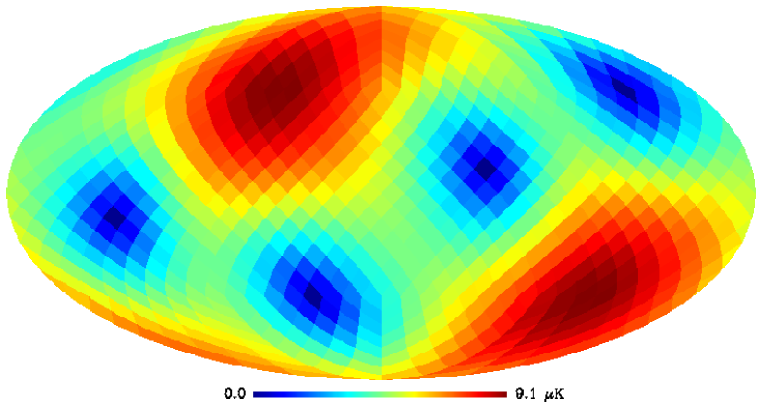
Figure 4: Full sky pattern (produced using the HEALPix package) of P/$\tau$ for redshift $z=0.034$ (our first slice). The 4 minima correspond to the 4 minima at 45 degrees of the hot and cold spot of the local CMB quadrupole, the 2 maxima correspond to the ones at 90 degrees.

The power on small scales is produced by the anisotropies in the optical depth $\tau$, and is increasing like $\ell^{0.5}$. The estimated power spectra by Hu (2000) and Cooray et al. (2004) (respectively orange dash-triple dotted and green dot-dashed lines on figure 3) match quite well our estimate on small scales ($\ell>100$). That is somewhat surprising as our reionization redshift is quite low : our simulation does not include structures at $z>2$ whereas the other estimates go at least to a redshift 5. We think that this match shows that our estimate have the same order of magnitude, but including higher $z$ may oncrease the signal further. The numerical estimate from Liu et al. (2005) is an order of magnitude higher than the semi-analytical results from Hu (2000) and Cooray et al. (2004), and from our own estimate. Our low reionization redshift could explain this discrepancy, the difference with Hu (2000) and Cooray et al. (2004) could lie in the details of their reionization model.
Another window on the polarized SZ signal is the polarization angle. On Figure 1, the polarization angle changes very slowly with the angular position (6.8 degrees in the 7.5 degrees field of view) especially at low redshift, as it is determined mainly by the angle between the line of sight and the CMB quadrupole direction. It also changes quite slowly with respect to the cluster redshift (Figure 5), due to the high correlation between quadrupole orientation at different redshift (the correlation length is about 0.1). It implies that one gains very little by measuring the quadrupole at different redshifts between 0 and 2 due to this large correlation (in agreement with Portsmouth (2004)). Furthermore, 2 clusters in the same direction but with different polarization angle will in fact be at different redshifts (like the 2 clusters in figure 1 at redshift 0.25 and 1.1), this difference in redshift being greater than the correlation length.

Figure 5: Average variation (over our 7.5$\times$7.5 degrees patch) of the $P/\tau$ (left) and of the polarization angle (right) versus redshift, error bars represent the 1 $\sigma$ dispersion of these values.

5 Conclusion

Compton scattering of CMB photons in the hot intra-cluster medium in massive halos generates a linear polarization proportional to the cluster optical depth and the local quadrupole of the CMB intensity. We have presented the first maps of this effect based on numerical simulations. With the procedure we have outlined in our simplified reionization model, the maps are accurate to 10%. Our simulations confirmed that the level of polarization due to this effect is rather small (a few tenth of $\mu$K), though we computed the effect only from sources at redshift lower than 2. The additional power coming from higher redshift would probably increase the statistical significance of the polarized SZ, but it should have little effect locally. We computed the power spectrum of our map and found similar results to Hu (2000) and Cooray et al. (2004). The polarization angle variation is dominated by the geometrical effect between the quadrupole direction and the observation direction, its value changes slowly in both angular position and redshift.

Acknowledgments:

We would like to acknowledge the use of the HEALPix package for our map pixellisation (Gorski et al., 1999) and thank our anonymous referee for usefull comments.

References

- (1)
- Amblard et al. (2004) Amblard, A., Vale, C. White, M., 2004, NewA, 9, 687
- Audit & Simmons (1999) Audit, E., Simmons, J.F.L., 1999, MNRAS, 305, 27
- Chluba & Mannheim (2002) Chluba, J., Mannheim, K., 2002, A&A, 396, 419
- Cooray & Baumann (2003) Cooray, A., Baumann, D., 2003, Phys. Rev. D, 67, 063505
- Cooray et al. (2004) Cooray, A., Baumann, D., Sigurdson, K., Proc. Enrico Fermi, International School of Physics Course CLIX, eds. F. Melchiorri & Y. Rephaeli, astro-ph/0410006
- Delabrouille et al. (2002) Delabrouille, J., Melin, J.-B., Bartlett, J.G., 2002, ASP Conference Proceedings Vol. 257., astro-ph/0109186
- Diego et al. (2003) Diego, J.M., Mazzotta, P., Silk, J., 2003, ApJ, 597, 1
- Gorski et al. (1999) Gorski, K.M., Hivon, E., Wandelt, B.D., (1999), in Proceedings of the MPA/ESO Cosmology Conference ”Evolution of Large-Scale Structure”, eds. A.J. Banday, R.S. Sheth and L. Da Costa, PrintPartners Ipskamp, NL, pp. 37-42 (also astro-ph/9812350)
- Hu (2000) Hu, W., 2000, ApJ, 529, 12
- Kamionkowski & Loeb (1997) Kamionkowski, M., Loeb, A., 1997, Phys. Rev. D, 56, 4511
- Liu et al. (2005) Liu, G.-C., da Silva, A., Aghanim N., 2005, ApJ, 621, 15
- Melin (2004) Melin, J.-B., 2004, Ph.D. thesis
- Portsmouth (2004) Portsmouth, J., 2004, Phys. Rev. D, 70, 063504
- Sachs & Wolfe (1967) Sachs, R., Wolfe, A., 1967, ApJ, 147, 73
- Sazonov & Sunyaev (1999) Sazonov, S.Y., Sunyaev, R.A., 1999, MNRAS, 310, 765