Extragalactic source counts in the 20–50 keV energy band
from the deep observation of the Coma region by INTEGRAL/IBIS

Abstract

We present the analysis of serendipitous sources in a deep, 500 ksec, hard X-ray observation of the Coma cluster region with the IBIS instrument onboard INTEGRAL. In addition to the Coma cluster, the final 20–50 keV image contains 12 serendipitous sources with statistical significance $>4\,\sigma$. We use these data (after correcting for expected number of false detections) to extend the extragalactic source counts in the 20–50 keV energy band down to a limiting flux of $1.0\times 10^{-11}$ erg s^-1 cm^-2 ($\simeq 1$ mCrab). This is a more than a factor of 10 improvement in sensitivity compared to the previous results in this energy band obtained with the HEAO-1 A4 instrument. The derived source counts are consistent with the Euclidean relation, $N(>f)\propto f^{-3/2}$. A large fraction of identified serendipitous sources are low-redshift, $z<0.02$ AGNs, mostly of Seyfert 1 type. The surface density of hard X-ray sources is $(1.4\pm 0.5)\times 10^{-2}$ per square degree above a flux threshold of $10^{-11}$ erg s^-1 cm^-2. These sources directly account for $\sim 3\%$ of the cosmic X-ray background in the 20–50 keV energy band. Given the low redshift depth of our sample, we expect that similar sources at higher redshifts account for a significant fraction of the hard X-ray background. Our field covers only 3% of the sky; a systematic analysis of other extragalactic INTEGRAL observations can produce much larger source samples and is, therefore, critically important.

1. Introduction

Most of the energy of the Cosmic X-ray Background (CXB) is emitted in the energy band around 30 keV (Marshall et al., 1980). However, the exact nature of the source population responsible for the background at these energies is unknown. The primary reason is low sensitivity of the previous X-ray telescopes operating above 20 keV. Studies of the high energy sources are also motivated by the recent work at lower energies, 2–10 keV. Most of the X-ray background at these energies is resolved into sources (Giacconi et al., 2002; Alexander et al., 2003) but the spectrum of those sources does not match that of the CXB at high energies, indicating the existence of a population of highly obscured sources, which should be detectable more easily above 20 keV (e.g., Worsley et al. 2004 and references therein).

The telescopes onboard INTEGRAL provide a major improvement in sensitivity for X-ray imaging above 20 keV (Winkler et al., 2003a). During its first year, INTEGRAL has conducted a number of deep pointings to the Galactic center region (Revnivtsev et al., 2004a) and the Galactic plane (Winkler et al., 2003b), as well as to several extragalactic targets. One of the deepest extragalactic observations was that of the Coma cluster region for a total exposure of 500 ksec. The Coma cluster is located very close to the North galactic pole and this field is minimally contaminated by the sources within our Galaxy which dominate the hard X-ray sky. In addition, the image is not “polluted” by a bright target and so it is excellent for detection of faint sources.

In this Paper, we report on the analysis of faint serendipitous sources in the Coma field. Our image reaches a $4\,\sigma$ detection threshold of 1 mCrab in the 20–50 keV energy band, above which we detected 12 serendipitous sources. Using this sample, we are able to extend the extragalactic $\log N-\log S$ in the hard X-ray band to a flux limit of $1.0\times 10^{-11}$ erg s^-1 cm^-2, a factor of $\sim 10$ deeper than the extragalactic part of the HEAO-1 A4 source catalog (Levine et al., 1984).

2. INTEGRAL observation of the Coma region

The Coma region was observed by INTEGRAL in 2003 on January 29–31 (revolution 36) for 170 ksec and on May 14–18 (revolutions 71–72) for 330 ksec. The observations consist of 221 shorter pointings which form a $10^{\circ}\times 10^{\circ}$ grid around the target with a $2^{\circ}$ distance between the grid points. The January and May datasets have different position angles, which leads to larger total sky coverage and helps to minimize the systematic residuals in the final image. The data quality in both series of observations is similar so they can be combined in a single $\sim$500 ksec dataset.

We used the data from IBIS/ISGRI instrument which is the most suitable for the imaging surveys in the hard X-ray band among the major instrument onboard INTEGRAL. IBIS (Ubertini et al., 2003) is coded-mask aperture telescope. Its CdTe-based ISGRI detector (Lebrun et al., 2003) has a high sensitivity above $20$ keV and has a high spatial resolution. The telescope field of view is $28^{\circ}\times 28^{\circ}$ ($9^{\circ}\times 9^{\circ}$ full coded). All Coma pointings cover a $40^{\circ}\times 40^{\circ}$ region.

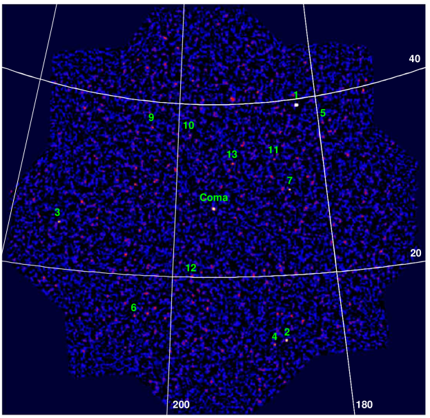
Figure 1.— X-ray image of Coma region in energy band 20-50 keV obtained by IBIS instrument onboard INTEGRAL during two different sets of observation. The color-coded intensity is in units of statistical significance for a point source. The markers indicate the locations of sources above a signal-to-noise level of 4.

3. Data reduction and image reconstruction

The IBIS data analysis involves special techniques for coded-mask image reconstruction, for which we used the software suite developed by one of us (EC). The essential steps are outlined below.

The event energies were calculated following the Off-line Scientific Analysis software v3.0 (Goldwurm et al. 2003) using the gain table v9 and the event rise time correction v7. Using the detector images accumulated in a broad energy band, we searched for hot and dead pixels and then screened the data to remove these artifacts. This resulted in rejection of several percent of the detector area. We then computed raw detector images for each pointing location and reconstructed the sky images individually.

The reconstruction starts with rebining the raw detector images into a grid with the pixel size equal to 1/3 of the mask pixel size. This is close but not exactly equal to the detector pixel size. Therefore, the rebining causes a moderate loss of spatial resolution but leads to straightforward application of the standard coded mask reconstruction algorithms (e.g., Fenimore & Cannon 1981, Skinner et al. 1987a). Basically, the flux for each sky location is calculated as the total flux in the detector pixels which “see” the location through the mask, minus the flux in the detector pixels blocked by the mask:

$$f=\sum_{M=1}D-BAL\sum_{M=0}D,$$ (1)

where $f$ is the source flux, $D$ is the detector image, $M=1$ or $0$ corresponds to transparent or opaque mask pixels, respectively, and $BAL\approx 1$ is so called balance matrix. The balance matrix accounts for non-uniformity of the detector background. For a given location it is calculated as:

$$BAL=\frac{\Sigma_{M=1}D_{b}}{\Sigma_{M=0}D_{b}},$$ (2)

where $D_{b}$ is the detector image accumulated over large number of observations without strong sources in the field of view (i.e., the background). Thus the expectation value of $f$ is zero for a source-free field (see eq. 1,2).

The images reconstruction is based on the DLD deconvolution procedure (see notations in Fenimore & Cannon 1981) when the mask pixel corresponds to $n\times n$ detector pixels. The original detector is treated as $n\times n$ independent detectors and $n\times n$ independent sky images are reconstructed and then combined into a single image. The point source in such image is represented by a $n\times n$ square. In our case, this leads to the effective Point Spread Function (PSF) being approximately a square of $3\times 3$ detector pixels or $12^{\prime}\times 12^{\prime}$.

Periodic structures in the mask produce sky images with a number of prominent peaks accompanying every real source. An iterative removal procedure was used to eliminate “ghosts” associated with the brightest sources (NGC 4151, NGC 4388 and Coma). No iterative removal of sources was performed for weak sources. The reconstructed images for each pointing grid location were co-added in the sky coordinates. Finally, we computed the statistical uncertainty of flux in the reconstructed image. This is a straightforward procedure because the noise is Poisson in the original data and it can be easily propagated through the image reconstruction algorithm (i.e., data rebining and DLD deconvolution).

We used the 20–50 keV energy band for detection of the serendipitous sources in the Coma field. The choice was motivated by the following considerations. The lower boundary of the energy range where IBIS is usefully sensitive is near 20 keV. The choice of the upper boundary is driven by the desire to extend the energy band to the highest energy possible without sacrificing the sensitivity. An upper boundary of 50 keV is a reasonable choice because at higher energies, the IBIS sensitivity rapidly decreases (Lebrun et al., 2003). We checked that at higher energies, there are no sources which are not detected in the 20–50 keV band. The reconstructed image is shown in Fig. 1.

4. Detection of Sources in the reconstructed image

Most of the extragalactic sources are very faint in the hard X-ray band. Their detection with INTEGRAL is challenging and requires sensitive techniques. Our approach is based on the so-called matched filtering technique. A similar method applied to the source detection in the ROSAT PSPC images is extensively described in Vikhlinin et al. (1995). We refer the reader to this paper and present only a brief overview below.

4.1. Matched Filter

The matched filter source detection is based on the convolution of the original image with the PSF. This method provides the most sensitive detection algorithm for finding faint, isolated sources (e.g., Pratt 1978). The only difference between the traditional matched filtering and our approach is to slightly modify the filter so that it can provide automatic background subtraction.

The image reconstruction algorithm for coded-aperture imaging implies, in principle, that the background in the reconstructed image is already subtracted (see eq. 1). However, some detector imperfections not fully accounted for by the balance matrix and other practical problems might lead to residual small-amplitude, large-scale intensity variations. The automatic background subtraction is therefore a desirable property of the detection algorithm.

The solution is to build the detection filter, $f(r)$, from two components. The positive component in the center matches the PSF and provides sensitive detection. The second one forms a negative “ring” at larger radii so that the average value of $f(r)$ is zero. We decided to implement $f(r)$ at the difference between the PSF and a Gaussian of larger width,

$$f(r)=P(r)-A\exp\left(-\frac{r^{2}}{2a^{2}}\right),$$ (3)

where $P(r)$ is the IBIS PSF, and the amplitude satisfies

$$A=\frac{1}{a^{2}}\int_{0}^{\infty}P(r)\,r\,dr.$$ (4)

The PSF calibration was obtained from the analysis of Crab observations. Crab is essentially a point source for INTEGRAL (the source size smaller than $4^{\prime}$ or 1 detector pixel), therefore its image can be used as a representation of the PSF (we actually used the average of 4 possible reflections of the Crab image around the $X$- and $Y$-axis to reduce statistical uncertainties). The derived PSF is essentially a square of $3\times 3$ pixels (or $12^{\prime}\times 12^{\prime}$) surrounded by fainter larger-scale wings; its one-dimensional slice is shown in Fig. 2.

Given the PSF, the only free parameter in the filter defined by eq. (3,4) is the Gaussian width, $a$. The choice of $a$ is driven by two conflicting requirements: a) the larger values of $a$ lead to better signal-to-noise (SNR) ratios in the convolved images, and b) smaller values of $a$ lead to more accurate subtraction of small-scale background variations. We chose $a=40^{\prime}$ which results in the signal-to-noise ratio of 99% of its maximum value (that for $\sigma\rightarrow\infty$).

Figure 2.— One-dimensional slice through the PSF of our reconstructed images after iterative source removal procedure (dotted histogram) and the profile of the detection filter (solid histogram). The pixel size is $4^{\prime}$. The PSF is the result of coadding of many real images (Crab Nebula) with different orientations. The resulting effective PSF is then more round and smooth than the ideal PSF (single pointing, no rebinning, perfect detector) which is a flat 3 by 3 pixels square in the DLD sky.

4.2. Source Detection, Fluxes, Locations

The sources are identified as local maxima in the the filter-convolved image. To sort out statistical fluctuations, we computed the convolved noise as

$$N(x,y)=\left((\text{noisemap})^{2}\otimes(f^{2})\right)^{1/2}.$$ (5)

This equation is strictly correct only if the individual image pixels are statistically independent, which is not fulfilled in our case because of rebinning of the detector images (§ 3). However, the effect is small because the correlation length of the noise in the reconstructed images is smaller than the size of the filter. It can be corrected by uniform rescaling of the noise map given by eq. (5) so that the rms variation of the ratio of the convolved image and $N(x,y)$ is 1. The required correction factors are $\approx 0.9$. Note that such adjustment effectively corresponds to noise determination directly from the data, which is the most trustworthy approach.

Accepted sources are the maxima in the convolved image with the signal-to-noise ratio $>~{}4$. This threshold is lower than what is often used in wide-area surveys. Our choice was motivated by the following considerations. Detection threshold is the result of compromise between our desire to exclude as many false detections as possible (this drives the threshold high) while retaining the maximum of real sources in the sample (this drives it low). The $4\sigma$ detection threshold results in manageable contamination of the sample by false detections, $4.7$ on average or $\sim 33\%$ of the total sample, which still can be reliably subtracted in the final $\log N-\log S$ analysis (§ 6.2).

Source fluxes can be obtained directly from filter-convolved images. The peak value in the convolved image is proportional to total source flux because convolution with the detection filter is a linear image transformation. The conversion factor between the peak value and flux was obtained using the reconstructed Crab images, for which we assumed the Crab spectrum $9.7\times E_{\text{keV}}^{-2.1}$ phot cm^-2 s^-1 keV^-1 (Toor & Seward, 1974). The conversion factor is a function of position because of several effects. First, the PSF degradation at large off-axis angles changes the peak value in the filter-convolved images. Second, off-axis PSF contains weak side-lobes which leads to over-subtraction of the source flux by a wavelet-like filter with a negative annulus, such as ours. Third, there is s vignetting effect most likely caused by absorption in the mask holes. These effects were calibrated using a large number of Crab observations with the source at different locations within the FOV. These observations were reduced identically to the Coma field. The derived peak-to-flux coefficient decreases by $22\%$ from $0^{\circ}$ to $5^{\circ}$ off-axis and then stays approximately constant. We used the conversion factor derived at $5^{\circ}$ and ignored the trend at smaller off-axis angles because it affects only a small fraction of the image area.

The source locations were measured as flux-weighted mean coordinates within $6^{\prime}$ of the maxima in the filter-convolved images. The accuracy of this method was tested using a large number of INTEGRAL observations in which there were sources with $\mathrm{SNR}=5-6$. The distribution of coordinate offsets for these sources is well described by a Gaussian with a 68% uncertainty radius of $4.2^{\prime}$.

The noise in the reconstructed image increases near the edge of the field of view. This region, if included in the survey, can pollute the source catalog with high-flux false sources. Therefore, we excluded the regions where the rms level of the image noise is a factor of 10 greater than that in the center of the field of view. This reduced the image area by 28%.

5. Detected Sources

Table 1Hard X-ray sources detected in the Coma field

X-ray ID	RA	Dec	Flux	SNR	Optical ID	Dist.	Type	$z$	$L_{x}$	ROSAT
	(J2000)	(J2000)	erg s-1 cm-2			arcmin			erg s-1
1	12 10 33	+39 24 21	$(3.2\pm 0.1)\times 10^{-10}$	44.5	NGC 4151	0.1	Sy1.5	0.0033	$7.3\times 10^{42}$	+
2	12 25 43	+12 40 42	$(1.1\pm 0.1)\times 10^{-10}$	9.5	NGC 4388	1.3	Sy2	0.0084	$1.6\times 10^{43}$
3	14 17 51	+25 08 43	$(5.3\pm 1.2)\times 10^{-11}$	5.1	NGC 5548	2.0	Sy1	0.0171	$3.3\times 10^{43}$	+
4	12 31 19	+12 14 01	$(5.2\pm 1.3)\times 10^{-11}$	4.7	$\cdots$	$\cdots$	$\cdots$	$\cdots$
5	11 56 47	+37 00 20	$(3.3\pm 1.0)\times 10^{-11}$	4.0	$\cdots$	$\cdots$	$\cdots$	$\cdots$
6	13 37 09	+15 20 00	$(2.9\pm 0.8)\times 10^{-11}$	4.1	$\cdots$	$\cdots$	$\cdots$	$\cdots$
7	12 18 23	+29 49 06	$(1.7\pm 0.3)\times 10^{-11}$	5.8	NGC 4253	0.8	Sy1	0.0129	$5.9\times 10^{42}$	+
8	12 59 35	+27 57 25	$(1.6\pm 0.2)\times 10^{-11}$	7.7	Coma	3.3	GClstr	0.0244	$2.4\times 10^{43}$	+
9	13 35 12	+37 12 17	$(1.5\pm 0.4)\times 10^{-11}$	4.1	V∗ BH CVn	3.0	CV	$\cdots$	$\cdots$	+
10	13 13 23	+36 34 20	$(1.6\pm 0.3)\times 10^{-11}$	4.6	NGC 5033	1.6	Sy1	0.0029	$2.4\times 10^{41}$	+
11	12 25 40	+33 31 13	$(1.4\pm 0.3)\times 10^{-11}$	4.2	NGC 4395	2.5	Sy1	0.0011	$3.0\times 10^{40}$	+
12	13 10 18	+20 01 51	$(1.1\pm 0.3)\times 10^{-11}$	4.2	$\cdots$	$\cdots$	$\cdots$	$\cdots$
13	12 48 49	+33 15 14	$(1.0\pm 0.3)\times 10^{-11}$	4.3	$\cdots$	$\cdots$	$\cdots$	$\cdots$

Note. — The uncertainty in the source locations is approximately $4^{\prime}$ (90% confidence). The fluxes and luminosities are in the 20–50 keV energy band.

Thirteen hard X-ray sources were detected above the $4\sigma$ threshold in our Coma image, including the target. The source locations and observed fluxes in the 20–50 keV energy band are given in Table 1. We searched for obvious optical identifications of our sources using the NASA Extragalactic Database as well as by the visual inspection of the images from Digitized Sky Survey and the ROSAT All-Sky Survey. Seven sources were unambiguously identified with the extragalactic objects (Table 1), most of them classified as Seyfert1 galaxies at low redshifts, $z<0.02$.

Our brightest sources were observed in hard X-rays with previous observatories (Macomb & Gehrels, 1999). NGC 4151 was observed with HEAO-1 A4 (Baity et al., 1984), SIGMA (Mandrou et al., 1994; Finoguenov et al., 1995), BeppoSAX (Piro et al., 1998), BATSE (Parsons et al., 1998). Seyfert-1 galaxy NGC 5548 was detected by HEAO-1 A4 (Rothschild et al., 1983), BeppoSAX (Nicastro et al., 2000), BATSE (Ling et al., 2000). NGC 4388 was detected by SIGMA (Lebrun et al., 1992) and BATSE (Bassani et al., 1996).

Most of positively identified INTEGRAL sources are also detected in the soft X-ray band in the ROSAT All-Sky Survey. The only exception is the Sy2 galaxy NGC 4388. This second-brightest INTEGRAL source is undetectable in the ROSAT energy band, most likely because of a high intrinsic absorption (Beckmann et al., 2004). One source (#9) is identified with the X-ray bright cataclysmic variable in our Galaxy. No identified sources have the same redshift as the Coma cluster, the observation target. Therefore, they are not located within the cluster or associated large-scale structures and we can safely use the entire sample to derive the serendipitous source counts.

We were unable to unambiguously identify 6 detected sources, partly because of the relatively poor positional accuracy achievable in the hard X-ray band. We note that some fraction of the unidentified sources are likely to be false detections as discussed below.

6. log N – log S for detected sources

6.1. Survey Area

Figure 3.— Survey area as a function of flux for sources with $\mathrm{SNR}>4$.

Since the image noise systematically increases at large off-axis distances, our detection threshold of $\mathrm{SNR}=4$ corresponds to different fluxes at different locations. Therefore, the survey area is a function of flux. This function is computed easily for the given noise map because the peak values in the convolved image is simply proportional to the source flux (see §4.2).

Equation (5) was used to obtain the noise map for the filter-convolved image. Multiplying this map by 4 and then by the flux conversion coefficient gives us the map of the minimal detectable flux, $f_{\text{min}}$, as a function of position. By counting the area where $f>f_{\text{min}}$, we obtain the survey area as a function of flux, $A(f)$. The results of this computation are shown in Fig. 3. The minimum detectable flux at the very center of the field of view is $0.9\times 10^{-11}$ erg s^-1 cm^-2 (or $\simeq 0.9$ mCrab). The survey area reaches its geometric limit of 1243 square degrees for $f>8.3\times 10^{-11}$ erg s^-1 cm^-2, and 50% of this area has the sensitivity better than $f=1.9\times 10^{-11}$ erg s^-1 cm^-2.

Given the survey area as a function of flux, $A(f)$, the cumulative source counts (also referred to as the $\log N-\log S$ distribution) can be computed easily as

$$N(>f)=\sum_{f_{i}>f}A(f_{i})^{-1}.$$ (6)

However, our source catalog must contain a small number of false detections because of the relatively low detection threshold ($\mathrm{SNR}=4$). We need to subtract their contribution from the $\log N-\log S$ measurement.

6.2. Expected Number of False Detections

The reconstruction algorithm for the coded-aperture images leads to the symmetric, Gaussian distribution noise in the resulting image. Therefore, the number of false detections (those arising because of noise) above a signal-to-noise ratio $\sigma$ can be estimated by counting the local minima with the amplitude below $-\sigma$.

The small number of the local minima with sufficiently high formal significance ($\mathrm{SNR}\lesssim-4$) is the main practical difficulty. We, therefore, adapted the following approach. We simulated a large number of images with the Gaussian noise, convolved them with the detection filter, and derived the distribution of the local maxima as a function of their formal significance, $\sigma$. The distribution was fit to a third-order polynomial in the $(\sigma,\log(dN/d\sigma))$ coordinates. The analytic model derived from simulations was slightly rescaled to match the distribution of local minima in the real data (Fig. 4).

Figure 4.— Distribution of the formal statistical significance of the local minima in the filter-convolved INTEGRAL image. The solid line shows the fit derived from Monte-Carlo simulations of the images with Gaussian noise, slightly rescaled to match the observed distribution.

The rescaled model allows us to predict the number of false detections as a function of the statistical significance threshold. We can also use it to predict the number of false detections as a function of limiting flux because we know the image noise as a function of position. Above our limiting flux, $1.0\times 10^{-11}$ erg s^-1 cm^-2, we expect 4.7 false detections, and 1.7 false sources above $2.8\times 10^{-11}$ erg s^-1 cm^-2. The expected average number of false detections is less than 0.1 at fluxes $f>10^{-10}$ erg s^-1 cm^-2. We can also compute the corresponding $\log N-\log S$ function for false sources using the survey sky coverage, identically to what is done with the real sources,

$$N_{\text{false}}(>f)=\sum_{i,j}\int_{\sigma_{\text{min}}}^{\infty}\frac{dN/d\sigma}{A(\sigma\,n_{i,j})}\,d\sigma,$$ (7)

where $n_{i,j}$ is the image noise in the pixel $(i,j)$, $\sigma_{\text{min}}=\mathrm{max}(4,f/n_{i,j})$, $A(f)$ is the sky coverage as a function of flux, $dN/d\sigma$ is the number of false detections in one pixel as a function of the formal statistical significance, and the sum is over all image pixels.

This procedure for estimating the number of false detections has been checked using shorter, 64 ksec, pieces of the Coma observation. Those sources detected in the short-exposure image and absent in the total 500 ksec image, are false. We verified that the $\log N-\log S$ for false sources predicted by eq. (7) for short exposures is in excellent agreement with that observed.

6.3. Results

Figure 5.— The $\log N-\log S$ distribution for the serendipitous hard X-ray sources in the Coma field. The histogram shows the source counts derived from the HEAO-1 A4 extragalactic sample ($|b|>30^{\circ}$). The HEAO-1 A4 fluxes were converted to our energy band from the nominal 25–40 keV band assuming a power-law spectrum with $\Gamma=2$. The dashed lines shows a $N\propto f^{-3/2}$ fit to our dataset.

Figure 5 shows the $\log N-\log S$ distribution for the serendipitous sources in the Coma field, corrected for the survey sky coverage as a function of flux, and subtracted contribution of false detections. Our results can be compared directly only with the previous measurements with the HEAO-1 A4 instrument which operated in the overlapping energy band, 25–40 keV (Levine et al., 1984).

The $\log N-\log S$ for the HEAO-1 A4 source catalog in the extragalactic sky ($|b|>30^{\circ}$) is shown by the solid histogram in Fig. 5. A single Euclidean function, $N(>f)\propto f^{-3/2}$, can fit both datasets. This is not surprising given that our sources are at low redshifts. For the fixed slope of the $\log N-\log S$ distribution at $-3/2$, we derive from our data only the surface density of the extragalactic hard X-ray sources $N=(1.4\pm 0.5)\times 10^{-2}$ per square degree above a limiting flux of $10^{-11}$ erg s^-1 cm^-2 in the 20–50 keV energy band.

All identified INTEGRAL sources have low redshifts, $z<0.02$. Therefore, the depth of our survey is small and it can be affected by the nearby large-scale structures. It would be extremely important to extend such measurements to a larger number of fields. However, it is interesting to note that, thanks to a greater sensitivity of INTEGRAL, the volume covered by our observation is larger than the volume covered by the extragalactic ($|b|>30\deg$) portion of the HEAO-1 A4 all-sky survey.

The all-sky catalog from the RXTE slew survey (Revnivtsev et al., 2004b) reaches a similar depth as our survey, although at a lower energy band of 8–20 keV. We can compare the number densities of sources by converting the RXTE fluxes to our energy band assuming a power law spectrum with $\Gamma=1.6$, the typical photon index for the RXTE AGNs (Fig. 8 in Revnivtsev et al.). The RXTE $\log N-\log S$ predicts the source density of $(0.9\pm 0.1)\times 10^{-2}$ per square degree above the flux limit of our survey; this is somewhat lower than, but within the uncertainties of, our measurement.

7. Discussion and conclusions

We have presented the analysis of the deepest hard X-ray image of the extragalactic sky obtained to date. We detected 12 serendipitous sources in the $40^{\circ}\times 40^{\circ}$ field centered at the Coma cluster. Most of the detected sources appear to be the Sy1 galaxies at low redshifts, $z<0.02$.

The $\log N-\log S$ distribution derived from a combination of our survey and extragalactic sample of the HEAO-1 A4 source catalog follows the Euclidean function, $N(>f)\propto f^{-3/2}$. The observed normalization of the $\log N-\log S$, $(1.4\pm 0.5)\times 10^{-2}$ per square degree above a limiting flux of $10^{-11}$ erg s^-1 cm^-2, corresponds to the integrated flux of $4.3\times 10^{-13}$ erg s^-1 cm^-2 deg^-2, or 3% of the total intensity of the hard X-ray background in the 20–50 keV energy band (Marshall et al., 1980).

The redshift depth of our source catalog appears to be below $z=0.02$. Therefore, it is reasonable to expect that the Euclidean source counts will extend to much fainter fluxes than our sensitivity limit. For example, the depth of $z<0.2$ where the space curvature of AGN evolution effects are still small, will correspond to approximately a factor of 100 lower flux. Extrapolation of our $\log N-\log S$ by a factor of 100 towards fainter fluxes will account for 30% of the total X-ray background in the 20–50 keV energy band. In short, we start to uncover the source population responsible for a significant fraction, if not most, of the hard X-ray background.

References

- Alexander et al. (2003) Alexander, D. M., et al. 2003, AJ, 126, 539
- Beckmann et al. (2004) Beckmann, V., Gehrels, N., Favre, P., Walter, R., Courvoisier, T. J.-L., Petrucci, P.-O., & Malzac, J. 2004, ApJ, 614, 641
- Baity et al. (1984) Baity, W. A., Worrall, D. M., Rothschild, R. E., Mushotzky, R. F., Tennant, A. F., & Primini, F. A. 1984, ApJ, 279, 555
- Bassani et al. (1996) Bassani, L., Malaguti, G., Paciesas, W. S., Palumbo, G. G. C., & Zhang, S. N. 1996, A&AS, 120, 559
- Butler & Scarsi (1990) Butler, R. C., & Scarsi, L. 1990, Proc. SPIE, 1344, 465
- Fenimore et al. (1981) Fenimore, E. E., Cannon T. M., 1981 Applied Optics, 20, 1858.
- Finoguenov et al. (1995) Finoguenov, A., et al. 1995, A&A, 300, 101
- Giacconi et al. (2002) Giacconi, R., et al. 2002, ApJS, 139, 369
- Goldwurm et al. (2003) Goldwurm, A., et al. 2003, A&A, 411, L223
- Levine et al. (1984) Levine, A. M., et al. 1984, ApJS, 54, 581
- Lebrun et al. (1992) Lebrun, F., et al. 1992, A&A, 264, 22
- Lebrun et al. (2003) Lebrun, F., et al. 2003, Astron. Asrtoph., 411, 141
- Ling et al. (2000) Ling, J. C., et al. 2000, ApJS, 127, 79
- Mandrou et al. (1994) Mandrou, P., et al. 1994, ApJS, 92, 343
- Macomb & Gehrels (1999) Macomb, D. J., & Gehrels, N. 1999, ApJS, 120, 335
- Marshall et al. (1980) Marshall, F. E., Boldt, E. A., Holt, S. S., Miller, R. B., Mushotzky, R. F., Rose, L. A., Rothschild, R. E., & Serlemitsos, P. J. 1980, ApJ, 235, 4
- Matt et al. (2000) Matt, G., Perola, G. C., Fiore, F., Guainazzi, M., Nicastro, F., & Piro, L. 2000, A&A, 363, 863
- Nicastro et al. (2000) Nicastro, F., et al. 2000, ApJ, 536, 718
- Parsons et al. (1998) Parsons, A. M., Gehrels, N., Paciesas, W. S., Harmon, B. A., Fishman, G. J., Wilson, C. A., & Zhang, S. N. 1998, ApJ, 501, 608
- Piro et al. (1998) Piro, L., et al. 1998, The Active X-ray Sky: Results from BeppoSAX and RXTE, 481
- Pratt (1978) Pratt, W. K. 1978, Digital Image Processing (New York: JW)
- Revnivtsev et al. (2004a) Revnivtsev, M. G., et al. 2004a, Astronomy Letters, 30, 430
- Revnivtsev et al. (2004b) Revnivtsev, M., Sazonov, S., Jahoda, K., & Gilfanov, M. 2004b, A&A, 418, 927
- Rothschild et al. (1983) Rothschild, R. E., Baity, W. A., Gruber, D. E., Matteson, J. L., Peterson, L. E., & Mushotzky, R. F. 1983, ApJ, 269, 423
- Skinner et al. (1981) Skinner, G. K. et al. 1987, Ap&SS, 136, 337-349.
- Toor & Seward (1974) Toor, A. & Seward, F. D. 1974, AJ, 79, 995
- Ubertini et al. (2003) Ubertini, P., et al. 2003, A&A, 411, L131
- Vikhlinin, Forman, Jones, & Murray (1995) Vikhlinin, A., Forman, W., Jones, C., & Murray, S. 1995, ApJ, 451, 542
- Winkler et al. (2003a) Winkler, C., et al. 2003a, A&A, 411, L1
- Winkler et al. (2003b) Winkler, C., et al. 2003b, A&A, 411, L349
- Worsley et al. (2004) Worsley, M. A. et al. 2004, MNRAS, in press (astro-ph/0412266)