Strong Lensing Analysis of A1689 from Deep Advanced Camera Images

Abstract

We analyse deep multi-colour Advanced Camera images of the largest known gravitational lens, A1689. Radial and tangential arcs delineate the critical curves in unprecedented detail and many small counter-images are found near the center of mass. We construct a flexible light deflection field to predict the appearance and positions of counter-images. The model is refined as new counter-images are identified and incorporated to improve the model, yielding a total of 106 images of 30 multiply lensed background galaxies, spanning a wide redshift range, 1.0$<$z$<$5.5. The resulting mass map is more circular in projection than the clumpy distribution of cluster galaxies and the light is more concentrated than the mass within $r<50kpc/h$. The projected mass profile flattens steadily towards the center with a shallow mean slope of $d\log\Sigma/d\log r\simeq-0.55\pm 0.1$, over the observed range, r$<250kpc/h$, matching well an NFW profile, but with a relatively high concentration, $C_{vir}=8.2^{+2.1}_{-1.8}$. A softened isothermal profile ($r_{core}=20\pm 2$^′′) is not conclusively excluded, illustrating that lensing constrains only projected quantities. Regarding cosmology, we clearly detect the purely geometric increase of bend-angles with redshift. The dependence on the cosmological parameters is weak due to the proximity of A1689, $z=0.18$, constraining the locus, $\Omega_{M}+\Omega_{\Lambda}\leq 1.2$. This consistency with standard cosmology provides independent support for our model, because the redshift information is not required to derive an accurate mass map. Similarly, the relative fluxes of the multiple images are reproduced well by our best fitting lens model.

1 Introduction

The puzzling “dark matter” phenomenon is strikingly evident in the centers of massive galaxy clusters, where large velocity dispersions are measured and gravitationally lensed arcs are often formed. Central cluster masses may be estimated by several means, leading to exceptionally high mass-to-light ratios, $M/L\sim 100-300h(M/L_{B})_{\odot}$, far exceeding both the stars responsible for the light of the cluster galaxies, and the mass of plasma implied by X-ray data. Reasonable consistency is claimed between dynamical, hydrodynamical and lensing-based estimates of cluster masses, supporting the conventional understanding of gravity. However, the high ratio of mass-to-light implies an unconventional non-baryonic dark material dominates the mass of clusters.

In detail, a discrepancy is often reported between the strong lensing and X-ray mass measurements, in the sense that X-ray masses are lower in the cluster center. This may be attributed to gas dynamics in unrelaxed cluster (Allen 1998) or perhaps to the current restriction on X-ray spectroscopy to energies below $\sim 8$KeV, which often falls short of the Bremsstrahlung cutoff for the massive lensing clusters, making temperature measurements uncertain and less direct. In many cases luminous X-ray clusters display merger induced effects (Markevitch etal 2002, Reiprich etal 2004) and surprisingly detailed structure in SZ maps has also been reported for RX1347-1145 (Kitayama etal 2004), although sometimes lensing and X-ray derived mass profiles are claimed to agree eg. MS1358+6245 (Arabadjis, Bautz & Garmire 2002). Lensing masses are often made uncertain by obvious substructures in the cores of massive clusters like A2218 (Kneib et al 1996), and weak lensing measurements are subject to observational problems (Kaiser, Squires & Broadhurst 1995) and an inherent mass profile degeneracy (Kaiser 1995, Schneider & Seitz 1995).

Simulations of massive clusters based on interaction-less cold dark matter are reliable enough to make statistical predictions for the mass profiles of galaxy clusters. A relatively shallow central mass profile is expected for cluster-sized haloes at the typical Einstein radius of $20-100h^{-1}kpc$. The gradient of an “NFW” profile (Navarro, Frenk & White 1996) continuously flattens towards the center, and for the most massive haloes is considerably flatter than a pure isothermal profile interior to the characteristic radius, but does not possess a constant density core in the center. The limiting inner slope of this profile seems to depend on the resolution of simulations, with somewhat steeper inner profiles claimed for more detailed simulations (Ghigna et al. 1998, 2000, Fukushinge& Makino 1997, Okamoto & Habe 1999, Power etal. 2003, Navarro etal. 2004), with an intrinsic variation in slopes predicted, related to variations in the assembly histories (Jing & Suto 2000, Tasitsiomi etal 2004). Other more radical suggestions include self-interacting dark matter (Spergel & Steindhardt 2000), for which the largest deviations should occur at high density, and hence this idea is amenable to investigation via strong lensing (Miralda-Escudé 2002).

Weak lensing has not yet provided any useful constraint on the mass profiles of galaxy clusters, with the best current data unable to distinguish a singular isothermal profile from the NFW model (eg. Clowe etal 2000). This unfortunately follows from the near degeneracy of weak lensing to the gradient of the mass profile. The shallower the profile the more magnified images become, but their shapes are hardly influenced, because the major and minor axes are stretched by nearly identical factors, virtually independent of the gradient of the mass profile. A firmer constraint may be made with magnification information, breaking the mass-sheet degeneracy, but this requires very deep imaging to overcome the intrinsic clustering of background galaxies or redshift information to filter the clustering along the line of sight (Broadhurst, Taylor & Peacock 1995). Measurements of magnification have so far proved noisy with ground-based data, so that the detection of this effect is currently restricted to only the most massive clusters (Fort et al. 1998, Taylor et al. 1998, Croom & Shanks 1999, Mayen & Soucail 2000, Rögnvaldsson et al.(2001), Athreya et al. 2002, Dye et al. 2002).

Strong lensing, leading to multiple images, occurs when the projected mass density of a body exceeds approximately $1.0g/cm^{2}$ (Turner, Ostriker & Gott 1981), producing elongated images of extended background galaxies (Paczynski 1986). This limit is surpassed it seems for nearly all distant clusters identified in deep survey work (Gioia et al. 1997, Gladders et al. 2003, Zaritski & Gonzalez 2003, Rosati et al. 2003) where giant arcs are commonly seen. However, at low redshift, z$<$0.1, many fewer clusters are known to display giant arcs. Here, lensing is harder to recognise because the isophotes of a low redshift central cD galaxy extend over a larger angular scale, exceeding the Einstein radius, which has only a weak dependence on the cluster redshift, thereby burying the main arcs. Only a few examples of giant arcs have been identified in nearby clusters, requiring ingenuity and careful extraction (Allen, Fabian & Kneib 1996, Blakeslee & Metzger 1999, Blakeslee et al 2001, Cypriano et al. 2001). Further work from space should perhaps be attempted given the detailed complementary information available on the internal dynamics and X-ray properties of the well studied nearby clusters.

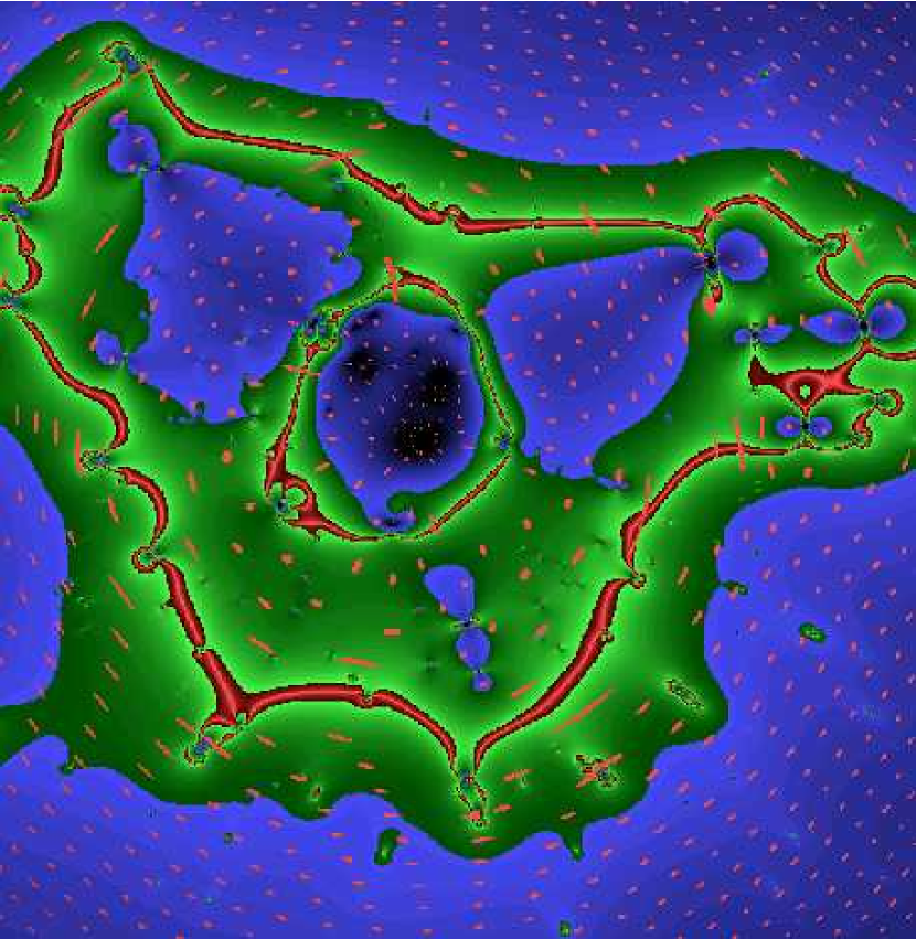
Figure 14: This figure illustrates the way images will appear to be distorted and magnified by our best fitting lens model. We generate the images from a grid of small circular sources using our best fit lens to re-map them onto the image plane. Overlayed on this plot is the magnification map, which is colour-coded to indicate the location of the critical curves and the relative strength of the magnification (for comparison with the next two similar figures). Note how a well defined radial critical curve appears here, highlighted by spoke-like images which bisect it, with much smaller less magnified images inside the radial critical curve.

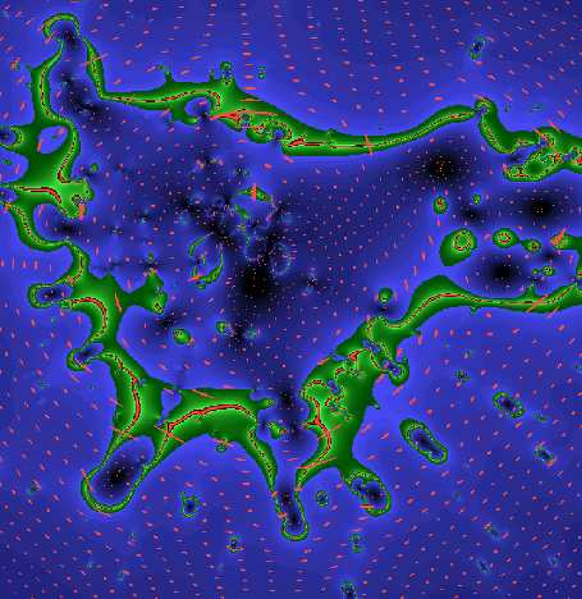
Figure 15: Same as the previous figure, but for a steeper mass profile, corresponding to the right-hand column of Figure 31. Here the magnifications of images interior to the tangential critical curve are relatively small and no distinct radial critical curve is generated, unlike the observations. The generally higher surface density of image reflects the generally small magnification by a steeper mass profile (for a fixed Einstein radius.)

It is important to appreciate that the vast majority of strongly lensed background galaxies do not resemble giant arcs and although images near the critical radius must be highly elongated, in practice they are often only marginally resolved, even in high resolution HST data. This is because the faint galaxy population is intrinsically small, FWHM $\sim 0.2$^′′at faint magnitudes, suffering pronounced, $\sim(1+z)^{-1.5}$, angular size evolution (Bouwens,Broadhurst & Silk 1998a,b, Bouwens et al. 2003). In the limit of point sources, like quasars, resolving the elongation is infeasible. Additionally, substructure in the cores of clusters complicates the appearance of arcs, so that images formed in regions between sub-clumps may be stretched roughly equally in all directions, leaving the shape of an image little affected, even if the source is highly magnified. This is also the case for images formed in an annulus lying between the radial and tangential critical curves, on the contour where the surface mass density is equal to the critical density (see for example, Figures 14,15&16), separating an inner region where images are radially directed from the outer area where they are predominantly tangential in shape.

The mass contained within the Einstein radius is given by fundamental constants and with knowledge of the distances involved and is therefore independent of the mass profile, provided the critical curve is approximately circular. Typically, significant asymmetry is evident and corrections must be made, though these are small in some favourable cases, for example the well studied clusters Cl0024+17 (Colley et al. 1995, Broadhurst et al. 2000), A370 (Bézecourt etal 1999) and MS2137 (Hammer et al. 1996, Kneib et al. 2002, Sand et al, 2002, Gavazzi et al 2003, Treu et al. 2003).

The clearest example of multiple lensing around a galaxy cluster is arguably the symmetric system identified around Cl0024+17, consisting of four tangential images lying on a nearly circular ring of radius $\approx 31$^′′ (Smail et al. 1994) and a small additional central image (Colley et al. 1995). These, together with a measurement of the redshift of the lensed system have been used to produce an accurate central mass for the region enclosing the Einstein radius, yielding a precise ratio for the center, $M/L(r<100kpc/h)=320\pm 20h(M/L_{B})_{\odot}$ (Broadhurst et al. 2000). In modeling this cluster, Broadhurst et al. (2000) find that the mass distribution closely follows that of the central luminous galaxies and the lensed images are readily reproduced in detail with only a modest number of parameters. A second pair of multiple images is identified for this cluster and predicted to lie at $z=1.3$, given their smaller relative deflection compared with the main system of arcs at $z=1.67$. Careful work has also been performed on a number of other clusters, most notably A2218, MS0404 and MS2137 (Kneib et al. 1996, Hammer et al., Treu et al. 2003, Gavazzi et al. 2003) for which two or three sets of multiple images are identified in each cluster, with varying conclusions regarding the mass profile depending on assumptions about the symmetry of the dark matter and the relative contribution of the central cD galaxy, which is particularly prominent in the case of MS2137.

Here we concentrate on A1689, which has the largest known Einstein radius of all the massive lensing clusters, of approximately 50^′′  in radius, based on the radius of curvature of a giant low surface-brightness arc. Relatively little work on this cluster has been carried out with HST, and the field of WFPC2 is too small to cover the full area interior to the Einstein radius. Although no actual multiple images had been identified prior to this investigation, we were confident that the exceptional depth and high resolution of the Advanced Camera would lead to the detection of many sets of multiple images, more than possible around other clusters, by virtue of the large Einstein radius.

We begin by describing the target selection ($\S$2), observations ($\S$3), and photometric analysis ($\S$4). We then visually identify the most obvious multiply lensed systems ($\S$5), allowing us to develop an initial mass model and refine the model in an iterative process. Section $\S$6 describes the 30 multiply-imaged sources we have identified. We integrate the cluster light ($\S$7) for comparison with our mass model. Section $\S$8 describes the actual procedure to construct the model. The resulting mass map, comparisons to other work, and cosmological implications are described in sections $\S$8-13. Finally, we summarise our conclusions ($\S$14). Note, throughout we adopt $H_{0}=100\,\textrm{km/s/Mpc}$ to allow comparison with earlier work.

2 Target Selection

The ACS Guaranteed Time Observations (GTO) program includes deep observations of several massive, intermediate redshift galaxy clusters. Our aims are to determine the distribution of the matter in clusters, to place new constraints on the cosmological parameters and to study the distant lensed galaxies, taking advantage of the large magnifications.

In selecting a target for a deep lensing study, we are not tempted to pursue the well known systems with notorious giant arcs. Instead we select our target principally by the size of the Einstein radius, in order to uncover as many multiply lensed background galaxies as possible. All background galaxies whose images fall within an area of approximately twice the Einstein radius will belong to a set of multiply lensed images, thus a larger Einstein radius will provide greater numbers of multiple images. With sufficiently deep multi-colour images of high spatial resolution, we may confidently integrate for long periods, secure that for systems of large Einstein radius many examples of multiply lensed background galaxies will be registered. For this reason A1689 is the preferred choice being the largest known lens, with an Einstein radius of approximately 50^′′, much larger than other better studied lensing clusters with typically only $\sim 15$^′′ radius, corresponding to a of factor of $\sim 10$ times more sky to a fixed magnification and hence a similar gain in the numbers of expected lensed galaxies around the Einstein radius, depending on the slope of the faint galaxy counts. In addition, the relatively low redshift of A1689 means we are not concerned so much with foreground contamination, thereby minimizing potential confusion when identifying counter-images.

We prefer to image deeply only a few clusters rather than make a larger survey, to secure significantly new information regarding the nature of dark matter. An approximate rule for cluster mass modeling is that the ‘resolution’ with which we can map the mass distribution depends on the surface density of multiply lensed images. To find many of these systems, the observations have to be deep. However, it is very difficult to get redshifts for galaxies fainter than $I\gtrsim 24.5-25$ even with the best instrument/telescope combinations available from the ground. In order to overcome this limitation, we have split our observations into 4 filters, $F475W$, $F625W$, $F775W$ and $F850LP$, in order to obtain reliable photometric redshift information, which may be compared with the known redshifts of some of these arcs that we have obtained already (Frye, Broadhurst & Benitez 2000).

3 Observations

A1689 was observed in June 2002 with the newly installed ACS on HST. The ACS images are aligned, cosmic-ray rejected, and drizzled together using the ACS GTO pipeline (Blakeslee et al. 2003). We utilise the full spectral range of the Advanced Camera, matching the relative depths of exposures in the g,r,i,z passbands to the relative instrumental sensitivity. In total we imaged 4 orbits in G and R and 3 in I and 7 in Z (see Table 1). We use the (09/25/02) CALACS zeropoints, offset by small amounts necessary for the errors present in this calibration. We reach $10\sigma$ magnitudes for point sources (inside a $4\times$FWHM aperture) of $27.5$ in the $g$ band, $27.2$ in the $r$ and $i$ bands, and $26.7$ in the $z-$band. Table 1 summarises the observations. The depth of the data and colour coverage are unprecedented for deep lensing work, and as we see below, sufficient for reliably identifying many sets of multiply lensed images. .

We complemented our ACS-based observations with $U-$band observations obtained with the DuPont telescope at Las Campanas Observatory, with a final PSF FWHM$=$0.59^′′ and also $J,H,K$ data at La Silla with the NTT telescope, with PSFs width of $\approx 0.8$ ^′′and AB limiting magnitudes of 24.21, 22.83 and 22.2 respectively. These datasets will be discussed in more detail in an upcoming paper (Coe et al. in preparation). Although they are far from matching the depth of our ACS data, nevertheless they are useful in improving our photometric redshifts for the brighter or redder galaxies.

4 Photometry

Photometry of faint objects in a cluster crowded field presents several challenges. The standard software for this task, SExtractor (Bertin & Arnouts 1996), cannot be applied directly to the images. The presence of bright, extended galaxies complicates the estimation of the real background, and even if this problem is solved by including an external background estimation, the software is not able to de-blend even moderately faint objects from the central cluster galaxies. To overcome this problem, we have carefully fitted and subtracted the central cluster galaxies. This process will be described in detail in an upcoming paper by Zekser et al. (in preparation). We combine the $g$, $r$, $i$ and $z$ images, weighting by the inverse of the variance of each image to create a detection image. After the bright galaxy subtraction, SExtractor produces a detection of most of the faint objects in this image, although in some difficult cases the apertures have to be defined manually. We measure isophotal magnitudes within these apertures, which have been shown to produce more accurate colours and photometric redshifts (Benítez et al. 2004). We use the same ACS-defined apertures for measuring magnitudes in the ground based images, correcting for the differences in the PSF using a new software we have developed (Coe et al., in preparation).

4.1 Photometric redshifts

We estimate photometric redshifts using the Bayesian based analysis code, BPZ (Benítez 2000) and the new set of templates introduced in Benítez et al. (2003). BPZ produces a full redshift probability distribution of the form:

$$p(z|C)\propto\sum_{T}p(z,T|m_{0})p(C|z,T)$$ (1)

where $p(D|z,T)$ is the redshift likelihood obtained by comparing the observed colours $C$ with the redshifted library of templates $T$. The factor $p(z,T|m_{0})$ is a prior which represents the redshift/spectral mix distribution as a function of the observed $I-$band magnitude. We use a prior which describes the redshift/spectral type mix in the HDFN, which has been shown to significantly reduce the number of “catastrophic” errors ($\Delta z>1$) in the photometric redshift catalog (see Benítez et al 2004 and references therein). We have modified this prior to adapt it to this particular catalog of objects, which are known to be background to the cluster and strongly magnified. The prior excludes the redshift range $z<0.7$, and assumes that the lensing corrected fluxes of the galaxies can be up to 20 times fainter than observed. The resulting redshifts for each individual arc are listed in Table 2. To obtain the redshift of the system, we take advantage of the Bayesian framework, and combine all the individual redshift probability distributions into a single probability for the system, $p(z|C)\propto\prod p_{i}(z|C)$, where $i=1,...,n$ corresponds to each of the multiple images. This may seem to have the same of effect of simply adding together all the observed fluxes and then estimating the redshift of the combined system. This would be the case if the only source of error in our photometric measurements were random noise, but unfortunately this is not so, in some cases, due to the presence of nearby residuals from the bright galaxy subtraction, our apertures are contaminated by spurious light, a problem especially common for the ground based observations. Combining the redshift probabilities together automatically “prunes” some of the spurious peaks, and quickly shows when one of the individual arc photometry is seriously contaminated and should be excluded from the redshift estimation for the whole system. The final redshifts for the whole systems are presented in Table 2.

5 Initial Multiple Image Identification

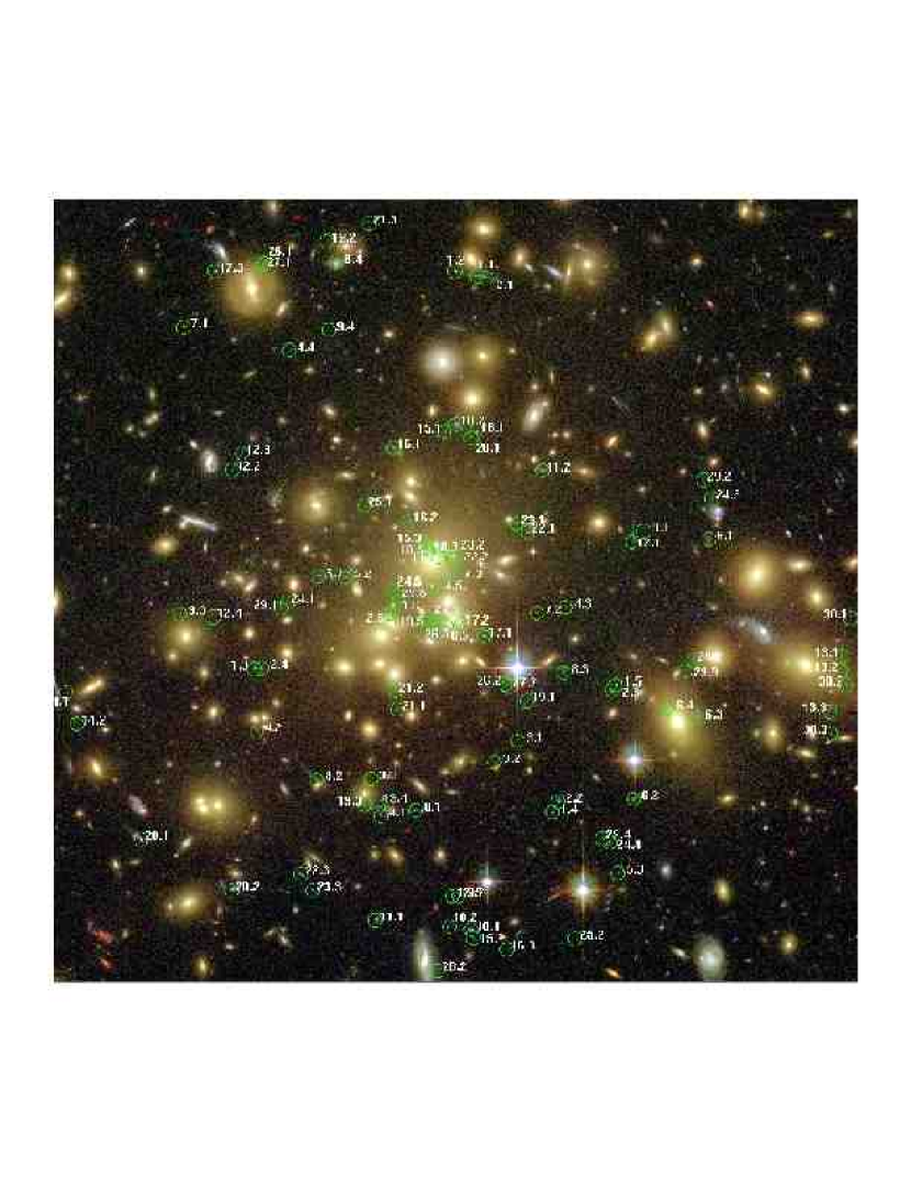
Figure 5: All 106 images identified to date with the help of the model are marked on the field of the data. Labels correspond to Table 2, where details of the photometry, coordinates, and redshift estimates are listed. The multiple images cover the cluster fairly evenly including the central region, interior to the radial critical curve. A closer view of the central region is provided below with the cluster galaxies subtracted.

Inspection of the colour image of the cluster provides, after some hours of scrutiny, several convincing cases of multiple imaging, which are later verified using the model. For example, the very red galaxy identified by Frye, Broadhurst & Benitez (2000) at z=4.9 (object $7.1$, Figure 5) has an obvious symmetrically placed counterpart of the same unusual colour in the form of a radial arc close to the center of the cluster (object $7.2$, Figure 5). The relative rarity of such bright red images adds confidence in this case. For bluer galaxies it is harder to choose between the many faint similarly blue background images and experience warns us that counter images can form in the most unlikely places. Small changes in the scaling of the bend-angle from the unknown source distance alters the location and even the formation of counter images, hence it becomes clear that the guidance of a useful model is needed to make reliable progress in reducing confusion. Redshift information is very useful as it helps narrow the range of allowable values of $d_{ls}/d_{s}$ when searching for counter-images. The high spatial resolution of ACS data enables morphological detail and internal colour variations to be used in identifying counter images. The generally complex morphology of faint galaxies means we can often identify unique internal features that must reproduce between images of the same source and must obey parity inversions. Usually some model guidance is needed here, as different arcs can be stretched along different directions, emphasizing different features.

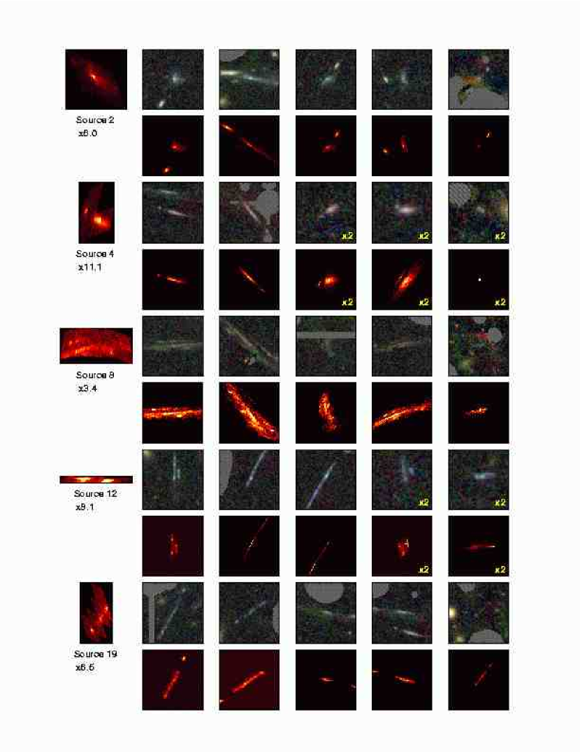
Figure 1: All sources lensed into five images are shown here in GRZ colour. Each set of multiple images is displayed along a single row. On the left of this row is the reconstructed source derived from delensing the first image in each row, usually the most magnified image. The source image is usally much smaller than its lensed images, so we show a magnified version relative to the lensed images (the magnification factor is printed on the stamp of the source). For comparison we generate the corresponding model images in a row below each set of observed images by applying the model to de-lens one of the observed images. We choose the R-band data of the most magnified multiple image - usually the first one in each row - to generate all the other images using the model. These model images generally match well their corresponding counter images, with little loss of resolution, demonstrating the accuracy of the model. This comparison is important to show when claiming a convincing model. Note that the model stamps are centered on the reconstructed image position for easy comparison with the data, and typically there is a small offset of the model image of $1-3$^′′  with respect to the observed image position, when using one image for generating the others (see section 8.4)

Some sets of images visible around the cluster are so unique that they are undoubtedly related. For example, five sets of images are visible as shown in Figure 1&2, labeled as objects 1&2. This system comprises a close pair of galaxies which is repeated four times around the cluster. A fifth pair of images is subsequently identified with the help of the model (see below, Section 6). One member has a secure redshift of z=3.05 (Frye et al. 2000). We will show below that our modeling places the other neighbouring image at a slightly lower redshift of z$\sim$2.5. Other images near to this pair can then be identified as multiple images, and then we may start on this limited basis to build a model.

6 Multiple Image Systems

Here we make notes regarding the individual sets of multiple images identified in the process of modeling (the modeling procedure is described in detail below). We include a table of their locations, photometric properties, and spectroscopic redshifts where measured. About one fifth of the lensed galaxy images described here were initially found by eye after careful scrutiny of the full colour image (see Figure 5), allowing an initial mass model to be constructed which in turn allows us to predict and verify the existence of more lensed images. When identified, these new images are added to refine the model in an iterative process, finally resulting in a robust mass model that reproduces nearly all of the lensed galaxy images accurately, in terms of their positions, morphology and relative magnifications. All the images identified by eye are confirmed by the model and the plausibility of model predicted images are examined carefully by eye.

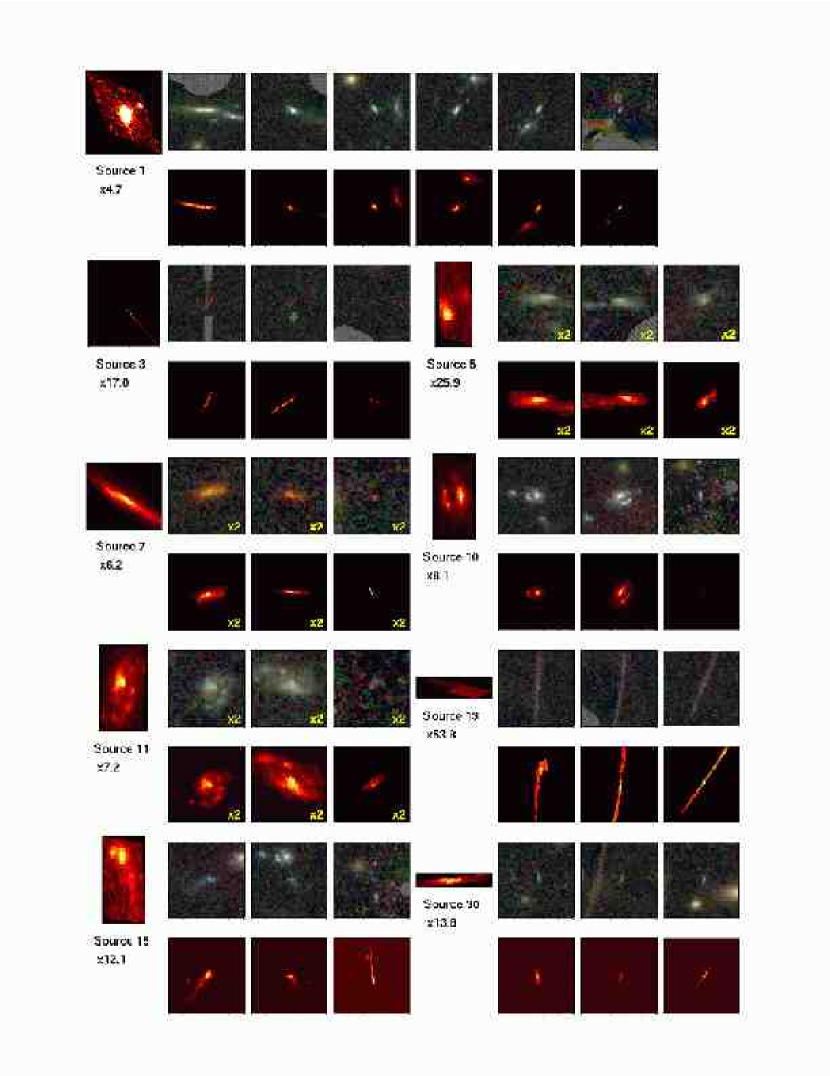
Figure 2: Similar to Figure 1. The first row here includes the source with the largest number of lensed images, 7 in total. Note the first postage stamp image of source 1 (labelled 1.1 in figure 5 and Table 2) is really two very closely spaced images which are split locally by a nearby cluster sequence galaxy. Interestingly, source 11 has a photometric redshift of z=2.9, and is clearly a well resolved spiral galaxy, magnified by a factor of $\sim 7$, and if the redshift is confirmed would be the highest redshift example of a galaxy displaying spiral structure.

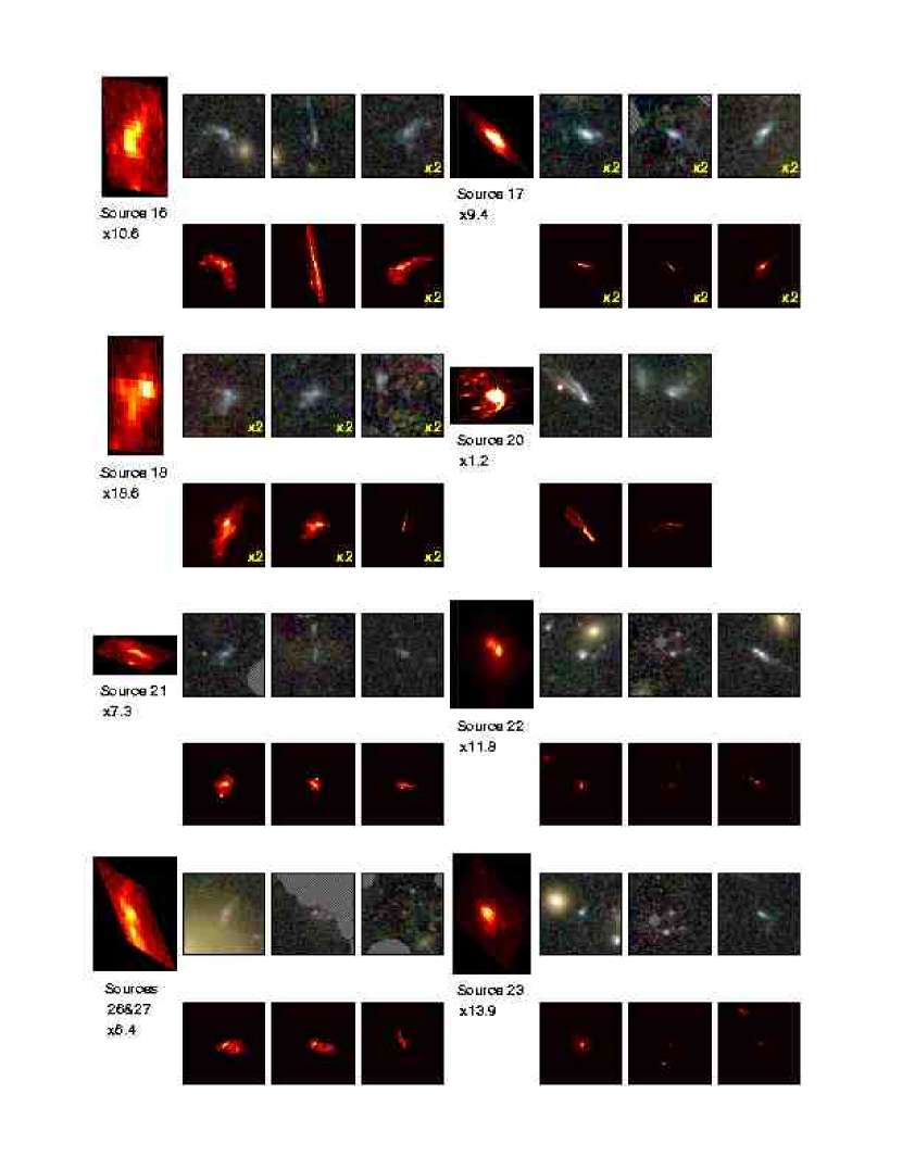
Figure 3: Similar to Figure 1. Comparison of observed and modeled multiple images found by our model. Observed images are shown above the corresponding model images and the reconstructed source is on the left.

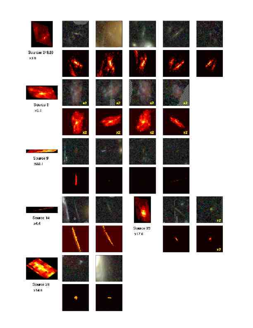
Figure 4: Similar to Figure 1. Comparison of observed and modeled multiple images found by our model. Observed images are shown above the corresponding model images and the reconstructed source is on the left.

Each set of images is shown in colour as a set of “postage stamps” in Figures 1–4, demonstrating rather obviously their relation to the parent source galaxy in most cases. Also shown alongside these observed images are the model generated images used to help identify counter images and scaled to the best fit deflection angle, $d_{ls}/d_{s}$. Also included is the de-lensed appearance of the source in the source plane, based on the most magnified image of a given source, which is placed in column 1, of Figures 1–4. The model images are generated by simply de-lensing one of the members of a set of images with the best-fit model for the deflection field, treating each pixel of the chosen input image as a set of pixels and not by mapping it first onto fixed grid in the source plane. This has the advantage that when re-lensing the source into the image plane to generate the model counter-images that the resolution is maximally preserved, as each pixel in the observed image can be re-mapped. This is obviously preferable to re-lensing a binned source plane, which would lead to a loss of resolution in the image place.

The stamps are shown with the same physical scale so they may be compared readily, except in the case of small images where we magnify the scale of the stamp, by an amount which we label on the stamp, in order to see the detail better. The source images are also shown magnified, usually by a factor of 5-10, so that their detailed internal structure revealed by lensing may be appreciated better. Corresponding observed and model-generated images typically agree to within 1-3^′′ for the best-fit model, so the position of each model stamp has been centered on the model image in figures 1–4, for a better comparison.

The resolution of our re-lensing procedure is matched to that of the data (i..e performed on a 4K grid, which is an effective limitation imposed by the FFT of the mass distribution when constructing the deflection field) and consequently the reproduction can look a little blurry in some cases. The image chosen for de-lensing is the first one in each row of multiple images shown in figures 1–4, and usually has a slightly sharper appearance than the rest, as it is simply a re-lensed version of itself. Usually we choose the largest image for this purpose since then information is generally only lost in creating the other smaller counter images. This does not work quite so well when the predominant lens stretching of a counter-image is not matched well in direction to that of the input image, especially if the source is intrinsically elongated orthogonally to the main direction in which an image is stretched as then the magnification of such images will emphasise different internal features, that may not be well resolved in the input image. Similarly, we have avoided where possible using input images which lie very close to caustics, since then the location of the caustic relative to the image must be known exquisitely well in order that the counter images and the source have meaningfully predicted shapes.

Photometric redshifts are estimated for all images and usually these agree well, with the exception of very faint counter-images, or in cases where there is light contamination from a neighbouring cluster galaxy. In the seven cases where we have spectroscopic redshifts, the agreement with the photometric estimate is good. These are of course generally bright images allowing successful spectroscopic redshift measurements, so the precision of the photometry is relatively good.

Sources 1 & 2

This is a close pair of galaxies separated by $\simeq 1$^′′ and identified four times around the critical curve with both radial and tangential parity reversals (see Figures 1,2,&5). The model is able to reproduce this pair of objects very well. Source 1’s images have a slightly larger deflection angle, requiring that it be slightly more distant than source 2. In addition, a de-magnified pair is predicted by the model to fall close to the cluster center of mass, lying within the radial critical curve. These two images are in fact identified close to the predicted locations with the correct sizes, relative orientations, and colours (stamp $1.5$ of Figure 1). The brightest image, $1.1$, is actually two closely split images due to the proximity of a luminous cluster member which locally perturbs the critical curve of the cluster. In total there are 7 images of source 1 and 5 of source 2, all fully accounted for by the model and with no additional images predicted by the model.

The redshift of image $1.1$ is known from many low ionization absorption lines in a very high quality Keck spectrum to be $z=3.05$ (Frye, Broadhurst & Benitez 2000) and is in good agreement with the photometric redshift estimate z=3.2$\pm$0.3. The spectrum also shows, rather unusually, 2 damped systems at lower redshift at $z=2.5$ and $z=2.3$. The photometric redshift for object 2 lying close to object 1, is estimated to be z=$2.5\pm 0.2$, and so $z=2.5$ is adopted when comparing the data with predictions of the model. One of the two damped systems in the spectrum of $1.1$ is very likely caused by extended gas associated with object 2, given their proximity. It is interesting to appreciate that this extended gas must cover a good fraction of the critical curve of A1689, following the distribution of the images of sources 1 & 2 around the whole lens. Deep narrow-band imaging tuned to Ly_α at the redshift of this damped system may be rewarded with a continuous emission map of the critical curves!

Source 3

There are 3 images of a very red dropout galaxy with a photo-z of z=5.3$\pm 0.4$. The most magnified images are a merging pair 3.1 & 3.2 crossing the critical curve. Two more images are predicted by the model. After subtracting an elliptical cluster member galaxy, we locate 3c, which is much fainter, as predicted, and lies close to our detection limit. A tiny counter image is also predicted on the opposite side of the cluster, however, this image is not identified and seems to lie below our threshold as we may expect based on its predicted flux which is a factor of 3 less than the barely-detected image 3.3.

Source 4

This is a distinctive high surface brightness galaxy with a clear internal colour variation, a point-like nucleus and an accompanying spot lying off one end. Four images are apparent, including the obvious mirror symmetric pair with reverse parity 4.1 & 4.2 and two smaller images confirmed by the model 4.3 & 4.4. This set of images corresponds to relatively small deflections, $\sim$15% smaller than that of images 1 & 2, and indeed the photo-z estimate is lower z=$1.1\pm 0.15$. This is an important set of arcs for the lens model, expanding the redshift range of the background sources and because its images lie all around the lens providing a tight constraint on the model. A central de-magnified image is predicted, 4.5, and is clearly identified by its characteristic colours (half red and half white) with the predicted parity. It lies close to the brightest cD galaxy.

Source 5

A pair of radially directed mirror images are seen close to the center of the cluster bisected by the radial critical curve. One counter image, 5.3, is predicted rather far off to one side of the lens and is readily identified near this position with the corresponding orientation, morphology and colour. The photometric redshift for this system is $3.2\pm 0.4$, indicating some flux has “dropped out” in the G band.

Source 6

Three very similar large images of an obvious disk galaxy with large internal colour variation and structure are seen associated with the main subgroup of the cluster. A fourth image, 6.4, is predicted by the model within the isophotes of a luminous cluster galaxy in this subgroup, and is readily found after subtraction of the cluster light (see Figure 4). This set of images has a reliable photometric redshift of $z=1.2\pm 0.15$. This set of arcs helps to constrain well the relative mass of the main sub-group of the cluster.

Source 7

A high surface brightness high redshift galaxy produces two prominent red images, one tangential (7.1) and one radial (7.2). The measured redshift of the brighter tangential image, 7.1, is z=4.9 (Frye, Broadhurst& Benitez 2000), in close agreement with the photometric redshift $z=4.8\pm 0.4$. The redshift of the radial counter image has also been measured and confirmed to lie at the same redshift (Bernard Fort priv. comm). A tiny central image is predicted and tentatively detected as the only red speck, 7.3, very close to the predicted position, near the most luminous cD galaxy. Deeper images would help clarify this along with many other small counter images in the center.

Source 8

This is a 4 image system with a similar arrangement to Source 4, but with a slightly larger set of bend-angles corresponding to a higher redshift source. A measured redshift of z=1.8 has been measured (Bernard fort, Priv. Comm). Images 8.1 & 8.2 are a continuous mirror symmetric pair of images forming the only giant arc around this cluster and bisected by the tangential critical curve at an oblique shallow angle (see Figure 1). A fifth image is predicted in the very center of the cluster and a likely candidate is identified by colour and shape near the predicted position (stamp 8.5 of Figure 1)

Source 9

This is another high-z dropout galaxy with a photometric redshift of $z=4.7\pm 0.4$. Image 9.1 is highly elongated and given its location requires that other multiple images should be formed. The model is essential here in finding the counter images. Three other images are predicted in total and all are securely identified close to the predicted locations. The shapes of the predicted images are not accurately matched which we blame on the proximity of the brightest image to the tangential critical curve in one of the most magnified regions of the lens (see Figure 1) and therefore the degree of stretching is enormous and not well aligned with the other images. This problem is very similar to that of object 12 which lies close by.

Sources 10,15,18

Two very similar looking blobby white images are seen on diametrically opposed locations and confirmed by the model, flanked by a pair of resolved blue objects. The photo-z of the brighter white object is $z=2.02\pm 0.3$. Two much fainter bluer neighbouring objects (objects 15 & 18) are also visible with photo-z consistent with z=2.02 which we may take to be independent galaxies with very similar redshifts to No. 10. The model shows that under this assumption the relative orientation and locations of this close triplet is consistent with all three objects being at the same distance, and thus nearly identically deflected. A third appearance of this set of three galaxies is predicted near the very center of the lens, as small images near the central cD galaxy and these are quite readily identified by their relative orientations and colours, and labeled 10.3,15.3 & 18.3.

Source 11

This is a pair of images of a nicely resolved spiral galaxy lying on opposite sides of the lens, with a photometric redshift of $z=2.9\pm 0.2$. One image is tangential and the other lies in the region between the radial and tangential critical curves where images are stretched roughly equally in all directions, producing a relatively undistorted image of the source which lies in the rather highly magnified region between the critical curves (see Figure 2 for relative magnification map) depending on the local slope of the mass profile. The model reproduces these very well, 11.1,11.2. A central image 11.3 is predicted and identified, close to the predicted position, with matching size, shape, colour and surface brightness. This may be the most distant known example of spiral galaxy, whose morphological identification is helped by the factor of $\approx 10$ in magnification.

Source 12

A giant blue arc with a mirror symmetric pattern forming two images 12.2 & 12.3 has a reliable redshift of z=1.83 from many emission lines with an AGN-type spectrum (Bernard Fort, priv. Com.). We predict this object to have 3 other images spread around the lens. One of these images, 12.1, has a redshift measurement in agreement with 12.2,12.3, with the same unusual emission line spectrum. The two other images predicted do not have redshift estimates, being much fainter but are readily identified. Note that this source has two components in the source plane which are resolved in images 12.1,12.4, and which are evidently elongated normal to a line connecting the two components and therefore form a continuous-looking image. Again the photo-z is in good agreement with the spectroscopic redshift (Table 2).

Source 13

A giant arc is located at the apex of the main subgroup of galaxies and on close inspection is resolved into three images straddling the tangential critical curve with a photo-z of $z=1.6\pm 0.2$. No other images are predicted by the model, as the source is evidently too far from the center of mass of the cluster. This source, together with source 30, helps fix the location of the critical curve around the outskirts of the the secondary group.

Source 14

A pair of closely separated highly elongated images 14.1 & 14.2 shows the location of the critical curve which they straddle. The photo-z for this object is $3.46\pm 0.3$, dropping out in the B-band. The close separation of these two images means that it does not significantly constrain the lens model, but it is very sensitive to the location of the critical curve which must pass between them.

Source 16

Two images of a very lumpy blue source are readily identified by their common morphology. Image 16.3 is highly radially stretched, but the model verifies that an elongated image can form at this location. The photo-z for this is $z=1.8\pm 0.37$.

Source 17

A close pair of radially elongated images of similar morphology are found straddling the radial critical curve, with a photo-z of $z=2.27\pm 0.25$. The predicted third image, 17.3, is readily identified close to the expected position with a morphology very close to the model prediction in shape and position angle on the opposite side of the lens.

Source 19

This source has two clearly related images 19.1,19.2 with a photo-z estimate of $z=2.7\pm 0.2$. The source is elongated in the direction of the shear for both of these two images. A close pair of images is predicted and stretched perpendicularly to the intrinsic elongation of the source. Close to the location of this predicted image is an obvious pair of closely separated mirror symmetric images, 19.3 & 19.4, but with colours which are slightly greener than 19.1 & 19.2 certainly due to contamination with images 8.1 & 8.2. A fifth image, 19.5, is also predicted to lie inside the radial critical curve close to the center of mass, and is readily identified by its orientation and elongated morphology. The photometric redshift is $z=2.7\pm 0.2$ (estimated for the uncontaminated images 19.1,19.2).

Source 20

Two relatively large images with similar internal colours and structure are found close to each other. The model convincingly reproduces the internal structure and relative locations. The photometric redshift is relatively low, $z\sim 1.57\pm 0.2$.

Source 21

A spotty blue radially stretched image is linked to two other images after the application of the model. The lumpy internal structure is replicated by the model and helps to correctly identify the counter images. The photometric redshift is rather uncertain for this faint blue object, with a most likely value of $z=1.86\pm 0.35$

Sources 22 & 23

Two high surface brightness poorly resolved sources lie close to each other and modeling shows that this pair is linked to two other sets of very similar images. The faintest pair lies interior to the radial critical curve. The outer pair is the brightest, and although these are considerably tangentially magnified they remain only marginally resolved, indicating the sources of these two objects are intrinsically very small (Figure 3). The photometric redshifts are consistent $z=2.24\pm 0.2$, in agreement with the model which finds their deflection angles have very similar scales.

Sources 24 & 29

A somewhat unusual pair of extended objects are confirmed by the model to form 5 pairs of images around the lens. The higher surface brightness object appears to be a barred galaxy and the low surface brightness accompanying smudge is not particularly galaxy-like in appearance. One image of this latter object falls amongst the massive galaxies of the main subgroup of cluster galaxies and forms a very highly magnified large trail spread between two of the massive galaxies. A small pair of counter images is predicted to lie within the radial critical curve and is readily identified close to the predicted location. A photometric redshift of $z=2.4\pm 0.3$ is measured. The appearance of this pair of images in the source plane suggests the source is one relatively large spiral galaxy with a large central bar.

Source 25

A large green radial arc bisecting the radial critical curve is identified using the model with a small barely resolved image of the same colour lying well outside the tangential critical curve. No more images of this source are predicted by the model. This case illustrates well the difficulty that one faces in identifying prominent radial arcs with shallow imaging data - the source is fortuitously located so that one image falls precisely on the radial critical curve forming a very magnified image whose counter image is much more modest, with a much smaller magnification. This object drops out in G and has a photometric redshift $z=3.79\pm 0.15$.

Sources 26 & 27

A close pair of pink and blue images are found at three locations forming 6 images. In one case the two images are coincident and seem to form one object. The distances of these two sources are not quite identical and indicate that these sources are unrelated, so that their relative positions can even overlap as seems to occur in the case, 26.3 & 27.3. For the combined object a photo-z of $z=1.7\pm 0.2$ is estimated, though from the modeling a very small difference in redshift may be expected between the blue and pink parts, corresponding to a difference of $\Delta{d_{ls}/d_{s}}\simeq 0.003$

Source 28

A very faint red galaxy with a counter image. Red lensed objects are scarce enough that identification is not very tricky - by running through a range of $d_{ls}/d_{s}$, the counter image is securely identified and has an estimated photometric redshift of $z=5.07\pm 0.3$.

Source 30

Three small green images lie close to the apex of the main subgroup following the tangential critical curve, the locations of which are accurately confirmed by the model. No other counter image of this source is predicted. A photometric redshift is estimated, $z=3.35\pm 0.2$.

7 Light Map

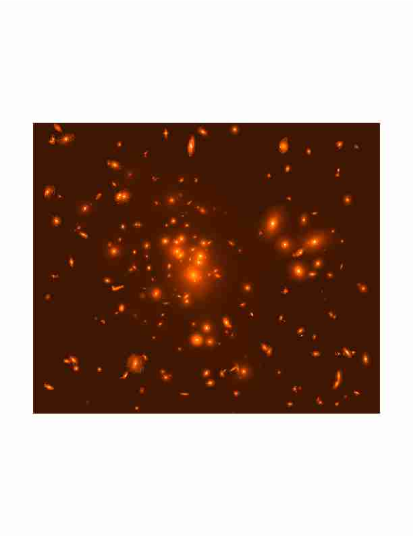
Figure 8: A 2-D map of the light generated by replacing the luminous early-type cluster galaxies with model profiles to trace their light to large radius free of sky noise. Also added to this map are luminous later type galaxies. These are directly cut out from the observed image rather than replaced with model profiles, because of their more complex structure. This 2D image is sued in calculating M/L profiles.

We have built a light map of the cluster in 2D so that we may make direct comparisons with the mass map. We start with the main cluster galaxies modeled as described in Zekser et al. (2004, in preparation). By making 2D fits to the cluster sequence galaxies we ensure that their haloes are modeled to large radii. In addition, we manually include those objects which, because of their colours or magnitudes, either belong to the cluster or may be in the foreground. We run SExtractor (in association mode) to generate an image which contains the flux belonging to these galaxies and is set equal to 0 elsewhere. Figure 8 shows the light map and the residual, background galaxy image, both obtained from the F475W image. To convert the observed AB F475W fluxes to B-band in the Johnson-Cousins systems we use the E/S0 and Sbc templates from Benitez et al. 2004, which yields filter corrections of 0.59 and 0.46 magnitudes respectively. Since we estimate that $80\%$ of the cluster galaxies have colours similar to E/SO galaxies, we use a weighted average correction of 0.565 for all the galaxies in the cluster, so $m_{B}=m_{F475W}+0.565$. Of this quantity, 0.12 mags correspond to the AB to Vega correction for the Johnson B filter. In a $\Omega_{m}=0.3$, $\Omega_{\Lambda}=0.7$ cosmology, the distance modulus at z=0.18 is 39.71, and the weighted k-correction for the $B_{Johnson}$ filter is 0.76 magnitudes, so $M_{B}=m_{f475w}-39.90$. We use $M_{\sun}=5.48$ to convert to solar luminosities: $2.179\times 10^{12}h^{-2}L_{\odot}$ within the ACS field of view. As a check, this may be compared with the catalog created by the ACS pipeline: after excluding all the stars and objects fainter than g=25, we obtain a total magnitude of $m_{F475W}=14.58$. This converts to $2.1\times 10^{12}h^{-2}L_{\odot}$, differing by only 3%.

8 Mass Modeling

The usual approach to lens modeling of galaxy clusters relies on many assumptions to describe the unknown cluster mass distribution and sub-cluster components. For any supposed cluster component, a center of mass must be designated, along with some ellipticity, positional angle, mass profile and normalization. This generates many largely unconstrained parameters and a degree of subjectivity in deciding what constitutes the main cluster and sub-components. The galaxy contributions may be better estimated from their location and luminosities, but the complications of dynamical interaction between galaxies and the cluster on the form of their mass profiles are of course unaccounted for in such idealised approaches.

The contribution of luminous cluster galaxies is not insignificant and must be included in any accurate modeling. The mass associated with a typical massive cD galaxy with a velocity dispersion of typically $\sim 300km/s$, may alone be expected to account for $\approx(300/1200)^{2}$ of the total mass, or $\sim 5\%$. The central location of such objects ensures they will influence the appearance of lensing. Cluster galaxies which happen to lie close to the Einstein ring can often be seen to perturb the location of lensed images, indicating masses amounting to a few percent contribution to the total mass interior to the Einstein ring (Franx et al. 1987, Frye & Broadhurst 1998). Of course, all galaxies in the cluster must be included at some level.

It is customary in lens modeling to specify the mass profiles of cluster galaxies in detail - including a profile, a core, a truncation radius, ellipticity and a scaling of these parameters with luminosity. Our preference, detailed below, is not to get bogged down in detail when specifying the galaxy contribution. As will become clear, it is in fact difficult in practice to motivate much more than simply the mass of a galaxy and its position in this context. This is principally because the deflection of light $\alpha(\theta)$, depends on the projected gradient of the gravitational potential, $\phi(r)$, so that any mass truncation radius is not distinctive, as the projected potential will drop off relatively slowly with angular separation from the center of mass, tending to the point mass limit, $1/\theta$, beyond any truncation radius. Interior to the lensing galaxy, the bend-angle will be approximately independent of radius if the mass distribution is approximately isothermal: $\alpha=4\pi{({\sigma\over{c}})^{2}}{d_{ls}\over{d_{s}}}$. Any core is very hard to constrain as images are nearly always deflected well beyond any reasonably sized small core. The ellipticity of the galaxy might be worth including, however this is usually small for the typical round shaped luminous cluster members and in any case the shape of the deflection field is a convolution of the projected mass distribution with angular separation, $\Sigma(\theta)\times 1/\theta$, hence the deflection field is intrinsically smoother and hence rounder than the mass distribution. Additionally, one has the uncertainty of converting the ellipticity of the galaxy isophotes into contours of surface mass density, along with any dependence of ellipticity on radius.

The hard part of the modeling is deciding how to deal with the general “dark matter” distribution of the cluster, which is understood to be the dominant component and is of course undetectably faint or invisible (by definition), so we have no direct visible guide to its distribution. We may begin with the simple expectation that mass should roughly follow light and develop an approach which avoids parameterization with idealised forms, but is based on the empirical distribution of the light in the cluster.

From previous experience with Cl0024+17 we have learned that a surprisingly good starting point for the shape of the general mass distribution may be obtained by simply using the luminous cluster galaxies and summing up extended profiles assigned to each one, producing a continuous 2D surface-density distribution (Broadhurst et al. 2000). We generalise this approach by dividing up the mass in to high and low frequency components, allowing a structured “galaxy” contribution and a smooth “cluster” component to be modeled independently. We do not iterate individual galaxy masses (following Broadhurst et al. 2000) as there are far too many galaxies in the strongly lensed region of A1689 to permit this. Instead we calculate the deflection field of the low frequency mass component and add a low order perturbation, since it has an intrinsically smoothly varying field light deflection field, unlike the more structured galaxy distribution. The contribution from the galaxy component is taken to be the difference between the smooth cluster component and the initial sum of galaxy mass profiles and is allowed freedom only in its normalization to approximately mimic the effect of changing the M/L ratio for the galaxy component.

Together, the perturbed low frequency “dark matter” component and the higher frequency “cluster galaxy” contributions constitute our lens model, which has the advantages of being very simple and flexible and is able to make accurate predictions for the location and appearance of counter images, so that the majority of the multiple images are identified by applying the model and all are confirmed using the model.

8.1 Starting Point for Lens Model

We begin by simply assigning an extended power-law profile to all cluster galaxies lying close to the E/SO colour-magnitude sequence. These are virtually all elliptical galaxies with only a handful of obvious disk galaxies. In total we select the brightest 246 objects to a magnitude limit of $I=23$, faintward of which, the background galaxies add confusion and are in any case at least 8 magnitudes fainter than the brightest cluster galaxy and do not add significantly to the overall mass. We have also verified that the exact choice of limit has negligible effect on the model. The profiles of the selected galaxies are not truncated but are run out to the edge of the field and beyond, to form a smooth general mass distribution tending to a 2D power-law profile at large radius. It is important to extend the mass distribution beyond the boundary of the data since the lensing deflection field that we wish to construct is not local but an integral over the surface of the cluster, falling off only slowly in projection by the angular separation, $1/\theta$. We start with this surface based on the light distribution of the cluster members and proceed as follows to break it into a smooth “dark matter” component which we iterate in shape, and a lumpy galaxy residual which we associate with the cluster galaxies and which is allowed to vary only in amplitude. We avoid additional unconstrainable parameters that only add to uncertainty in the model. The steps taken are as follows:

For each cluster galaxy a symmetric power-law surface density profile, $\Sigma(r)=Kr^{-q}$, is integrated to give the interior mass, $M(<{\theta})={{2\pi K}\over{2-q}}{d_{l}\theta}^{2-q}$, leading to a bend-angle of light:

$$\alpha(\theta)={4GM(<\theta)\over{c^{2}}\theta}{d_{ls}\over{{d_{s}}{d_{l}}}}$$ (2)

or

$$\alpha(\theta)={CD\over{2-q}}\theta^{-q+1}$$ (3)

where we separate the normalization, $C=8\pi KG/c^{2}$, from the distances, $D=d_{ls}d_{l}^{1-q}/d_{s}$.

We simply scale the normalization, $C$, to the luminosity of each galaxy. (One could experiment with more complex scaling of M/L with M, though a linear relation seems to be indicated by recent statistical work (Sheth et al. 2002, Padmanabhan et al. 2002, although see Guzik & Seljak 2003). Once the surface mass distribution is constructed from the sum of the above profiles then the deflection field can be derived and is initially used to crudely represent the combination of galaxies and the cluster together, implicitly assuming that the mass of the cluster traces the light:

$$\vec{\alpha}_{T}(\vec{\theta})=\Sigma_{i}\vec{\alpha}_{i}(\vec{\theta})$$ (4)

This deflection field is our starting point and is now broken down into a smooth component, $\vec{\alpha}_{s}(\vec{\theta})$ to represent the overall cluster mass distribution, and a lumpy residual component, to represent the cluster sequence galaxies $\vec{\alpha}_{g}(\vec{\theta})=\vec{\alpha}_{T}(\vec{\theta})-\vec{\alpha}_{s}(\vec{\theta})$. These contributions are varied separately in conjunction with the positions of the multiple images to generate the model fit, as described below.

8.2 Cluster and Galaxy Components

The locations of the cluster galaxies should serve as a rough tracer of the overall mass distribution and so we take the low order 2D function to generate a smooth surface mass distribution as a starting point for modeling the dominant smooth cluster component. We have tested a variety of smooth surface fits of varying resolution and settled on cubic splines of order 5-8. Higher order fits are unreasonably structured and produce many more multiply lensed images than are observed, and with lower order a virtually featureless circular mass profile is produced requiring large perturbations to match the data that are hard to control.

The deflection of light received at any angular position can then be calculated by a convolution of the surface mass profile with a $1/\theta$ kernel. The contribution to the angle, $\vec{\alpha}(\vec{\theta})$, by which light is deflected at angular position, $\vec{\theta}$, by a small mass element, $dm=\Sigma(\vec{\theta}{{}^{\prime}}){d^{2}\theta{{}^{\prime}}}$, separated by , $\Delta\theta$, can be approximated as a point mass deflection, $d\alpha={dm\over{\Delta x}}{d_{ls}\over{d_{s}}}$, where, $\Delta x={d_{l}}\Delta\theta$, is the projected separation in the lens plane, i.e. $d\alpha={dm\over{\Delta\theta d_{l}}}{d_{ls}\over{d_{s}}}$, and integrating this over the mass distribution in the full lens plane, allows the full deflection field to be calculated:

$$\vec{\alpha}_{s}(\vec{\theta})={4G\over{c^{2}}}{d_{ls}d_{l}\over{{d_{s}}}}\int_{R}\Sigma(\vec{\theta}^{{}^{\prime}}){\vec{\theta}-\vec{\theta}{{}^{\prime}}\over{|\theta-\theta{{}^{\prime}}|^{2}}}d^{2}\theta{{}^{\prime}}$$ (5)

In practice this deflection field is calculated by FFT by first binning the mass distribution onto a 1024$\times$1024 grid and repeating it 16 times in a 4$\times$4 array so that the deflection field calculated by FFT is completely free of any evidence of spurious boundary effects. The resulting deflection field is then numerically interpolated by a factor of 16, using the gradients of the local deflection field, to match the spatial resolution of the data. This high resolution is essential for making a proper comparison of the observed images with the model generated lensed images, as described below. Note, we calculate the deflection field over a wider area than covered by the data, extending the summation of the mass profiles to cover an area twice the size of the data field in order to deal with the edge effects since the deflection field is not local and so this way we minimise the edge effects in the calculation described by Eq. 5.

The full deflection field is required for iterating the relationship between the unknown source position, $\vec{\beta}$, and the image via the lensing equation, i.e.

$$\vec{\theta}=\vec{\beta}+\vec{\alpha}{(\vec{\theta})}{d_{ls}\over{d_{s}}}$$ (6)

The most practical part of our procedure is the use of the deflection field in the model iteration. The reason we choose this rather than the input mass distribution is twofold. Firstly, the deflection field is always smoother than the mass, as can be readily seen from the convolution above, $\Sigma(\theta)\times{1\over{\theta}}$ (Eq. 5) and hence more smoothly perturbed than the mass distribution. In addition, the deflection field must be calculated in the process of minimization as it is required so that the bend-angles of the model generated multiple image locations can be predicted.

The angular diameter distance ratio of each source, $D_{k}(z)=d_{ls}/d_{s}$, scales with redshift and acts simply to scale the amplitude of the deflection fields. However since the normalization of the surface density distribution also acts to linearly scale the bend-angles then distances can not be known separately from the density normalization i.e. $\alpha\propto\Sigma_{o}d_{ls}/d_{s}$, we must therefore work only with relative bend angles. Hence we define a convenient fiducial value of $D_{o}\equiv d_{ls}/d_{s}(z=3)$, corresponding to the mean redshift of the background galaxies $z=3$, and define the relative distance ratios to be:

$$f_{k}\equiv D_{k}(z)/D_{o}$$ (7)

This relative ratio is referred to in the minimization below and also used for comparison with cosmological models discussed in section 13.

8.3 Iterating the Deflection Fields

We treat the perturbation as a modification of the gravitational potential and use the orthogonal derivatives of this perturbation to modify the deflection fields to avoid introducing any curl, so that the smooth components of the deflection fields become:

$$\alpha_{s_{x}}{{}^{\prime}}(\vec{\theta})=\alpha_{s_{x}}+\frac{\partial P(\vec{\theta})}{\partial\theta_{x}}$$ (8)

$$\alpha_{s_{y}}{{}^{\prime}}(\vec{\theta})=\alpha_{s_{y}}+\frac{\partial P(\vec{\theta})}{\partial\theta_{y}}$$ (9)

The coefficients of $P(\theta)$ are free parameters in modeling the shape of the smooth cluster component. We use plain polynomials as only a low order perturbation is required (3rd or 4th order) and we prefer not work in polar coordinates as this imposes a spurious multi-pole pattern on the deflection fields at low order.

Two additional free parameters are required, to allow the galaxy contribution to vary in amplitude, $R$,

$$\vec{\alpha}_{g}{{}^{\prime}}(\vec{\theta})={R}{\vec{\alpha}_{g}(\vec{\theta})}$$ (10)

with an overall normalization, $A_{o}$, of both components, i.e.

$$\vec{\alpha}_{T}{{}^{\prime}}(\vec{\theta})=A_{o}(\vec{\alpha}_{s}{{}^{\prime}}(\vec{\theta})+\vec{\alpha}_{g}{{}^{\prime}}(\vec{\theta}))$$ (11)

Finally, the resulting surface mass density distribution, $\Sigma{{}^{\prime}}(\vec{\theta})$, responsible for the iterated deflection field, $\vec{\alpha}{{}^{\prime}}$, is obtained very simply via Poisson’s equation, since the bend-angle is the gradient of the projected potential and therefore the surface density is simply:

$$\Sigma{{}^{\prime}}(\vec{\theta})={1\over 2}\Sigma_{crit}\vec{\nabla}\cdot\vec{\alpha}_{T}{{}^{\prime}}(\vec{\theta})$$ (12)

This rather general approach to parameterising the model leads to results which are relatively free of assumptions. We emphasise again that division of the surface mass distribution into low and high order components is not meant to correspond literally to a division between cluster dark-matter and the galaxy masses, but rather that their combination is a description of the entire mass distribution. This resulting surface mass distribution may if desired be subsequently divided into galaxy and cluster contributions following a plausible model, which we do not attempt here. A follow-up paper treats this subject, beginning with an NFW profile for the smooth cluster component (Zekser et al. 2004).

8.4 Minimization

The simplest measure of the accuracy of the model is to compare model predicted image positions, $\vec{\theta}^{m}_{i,k}$ with the observed image locations, $\vec{\theta}_{i,k}$ and thereby avoid the pitfalls of working in the source plane (Kochanek 1991). For each of the N sources we have M multiple images, forming in total N$\times$M images to constrain the model. Ranking the M images of each source, we subtract in turn the model deflection angle from the each image of each source, k, and assign these a value of k, on a grid in the source plane, all other grid points are zero by default. Then the source plane is re-lensed but only for a relatively small box around each of other, M-1, observed image positions, saving time, and the model positions are recorded if all the re-lensed images of all the sources appear in these boxes. This process is repeated for each of the other M-1 images of each source and finally we sum over the differences between all the pairs of measured image positions and their corresponding model generated positions to form a measure of the accuracy of the model, which is simply expressed as:

$$\chi^{2}_{im}=\sum_{k}\sum_{i,j,i>j}\left({\vec{\theta}_{j,k}-\vec{\theta}^{m}_{j,k}}\right)^{2}$$ (13)

The above flagging of the source belonging to each set of images means we can identify the model image location of the correct source, avoiding confusion between counter images of different sources. The whole image plane does not need to be scanned for images as we are only interested in cases where the predicted images form close to the actual observed positions. In practice a box of side 5^′′ is sufficient to include nearly all the counter image positions while converging to a solution in a reasonable time. The number of iterations is reduced considerably by terminating an iteration when the variation between the source positions of a given set of multiple images is unreasonably large and moving to the next iteration step.

In this process we set all the relative distances to be equal, $f_{k}=1$, since, as we shall show below the best-fit model is negligibly affected by the choice of $f_{k}$. The search box must also be large enough to allow for some variation in the unknown distances, $d_{ls}/d_{s}$, which as we show below are reasonably expected differ by up to $\sim$ 15% in angular scale over the redshift range of the background sources. This range is small because of the relatively low redshift of A1689, $z=0.185$ so that only slow redshift dependence of $d_{ls}/d_{s}$ is expected for $z>1$ (see section 8.5), where the bulk of the faint lensed galaxies lie, i.e $d_{ls}\simeq d_{s}$ for z$>$1.

We have applied the “downhill simplex” algorithm (Press et al.) to find a minimum and this solution has been compared with a crude grid search as a sanity check. We have found that 9-14 coefficients are preferred for the perturbing potential to achieve considerable model flexibility (equation N), corresponding to third or fourth order with cross terms. Adding more terms seems not to be justified, with little noticeable improvement of any relevant quantities.

We have plotted $\chi^{2}_{im}$, calculated above for different choices of the input slope, $q$, and plotted this against the mean slope of the resulting mass profile, $\bar{p}=d\log\Sigma(\theta)/d\log\theta$, as this is the major quantity of interest. We find a clear minimum in the difference between the model and observed image locations for a slope around $\bar{p}\sim-0.55$, corresponding to $q=-1.2$. For steeper slopes the error increases and the disagreement with the data is pronounced in the center where the radial critical curve breaks up into small islands. For flatter slopes, $\chi^{2}$ is larger and the elongation of the lensed images becomes large and additional unobserved tangential images form readily as the area of the image plane close to the critical density is enlarged and upward fluctuations from the galaxies lead to exaggerated arcs. In the center, a flatter slope also produces much longer and fatter radial arcs than are observed, with a deficit of central de-magnified images, these being pushed outward too far in radius compared with the observed images. We include 3 model figures to demonstrate this behaviour, showing the locations, sizes and shapes of the lensed images compared to the critical curves for three different choices of input profile slope (Figures 14,15&16).

Note that the input slope of the galaxy profiles is generally steeper than the resulting mass profile of the cluster, simply because the galaxies are spread over the surface of the cluster and are not concentrated at one point in the middle.

We emphasise here that the slope of the mass profile is the main parameter of interest for comparison with predictions of N-body codes etc. The overall gradient of the profile has a noticeable effect on the appearance and location of images, as described above and, as we shall see later, on the relative distances and relative magnifications predicted for the background lensed galaxies, which we will compare with the observed redshift information (in sections 9 and 13). The parameters of the model are coupled somewhat in that the initial choice of the slope, q, of the galaxy profiles used to build the starting surface will determine what fraction of the mass is assigned to the “galaxy” and “cluster” mass components, and hence the relative fractions should not of course be taken as literal division into cluster and galaxy mass contributions.

We express our results in terms of the resulting profile of the mass distribution because the profile is the quantity of interest for testing physical models for the dark matter. Note that N-body simulations include the full spectrum of density perturbations, so that galaxies are included by default in the derived profile of the overall mass profile of clusters and therefore when making comparisons of mass profiles with the results of N-body simulations, it is preferable not to remove the galaxy contributions - with the exception only of the small baryonic component. If desired the resulting model surface mass distribution can of course be decomposed into “galaxy” and “cluster” contributions, following reasonable assumptions and will be explored in a subsequent paper (Zekser et al. 2004, in preparation).

8.5 Role of lensing distance ratio

We can make use of the best fitting model deflection fields to calculate the corresponding values of $f_{k}$ predicted by the model. The scale of the deflection field grows with increasing source distance and hence we can form a statistical measure of $f_{k}$ by calculating the angular separations between images:

$$f_{k}={1\over{(n_{k}-1)^{2}}}\sum_{i,j,i>j}{{(\vec{\theta}_{i,k}}-{\vec{\theta}_{j,k})}\cdot{(\vec{\alpha}{(\vec{\theta}_{j,k})}-\vec{\alpha}{(\vec{\theta}_{i,k})})}\over{(\vec{\alpha}{(\vec{\theta}_{j,k})}-\vec{\alpha}{(\vec{\theta}_{i,k})})^{2}}}$$ (14)

This useful expression shows that $f_{k}$ scales in amplitude as the ratio of the observed image separations divided by the predicted model image separations, as one might anticipate, since the larger the value of $f_{k}$, the larger the deflection angle $\propto{\vec{\alpha}(\theta)}{d_{ls}/d_{s}}$. The output values of $f_{k}$ span a plausible range of relative distances $0.8<f_{k}<1.1$, with the fainter red dropout galaxies lying at larger predicted distances than the brighter, lower redshift objects (Figure 12).

The output values of $f_{k}$ shown in figure 12 are produced by setting all of the distances equal. Here we investigate the dependence of the output $f_{k}$ on the choice of input values for $f_{k}$. We generate random values for the input $f_{k}$ and look at the corresponding output values. The size of the scatter on the input values $f_{k}$ was varied by 30%, more than covering the range anticipated from the cosmological variation (discussed in section 8.5). Figure 12 shows multiple trials of random sets of initial values assigned to the k sets of multiple images, showing clearly that the scatter on the model derived $f_{k}$ is small $\simeq 0.01$ per image, much smaller than the range of output, $f_{k}$, calculated as above (eqn 14), and with an average value very close to the input value of unity. Hence, we can be confident that we do not need to leave the values of $f_{k}$ free in our modeling, and incur many more free parameters in the minimization, but we can fix them at a desired mean level initially and use the resulting model to calculate accurate $f_{k}$ using eqn 14. This shortcut is possible because of the large number of background sources and because the mass distribution obtained is more based on the average redshift when the lens plane is covered by many multiple images. The mass distribution of the lens is of course independent of $d_{ls}/d_{s}$, and so must be the same no matter the distances of the background sources.

9 Relative Magnifications

We can compare the relative magnifications of the multiply lensed images with the model predicted values using the results of the above section. The relative magnifications are quite sensitive to the profile, as shown in figures 14,15,&16, and since this is the main quantity of interest for comparison with physical descriptions for the dark-matter distribution, we make a detailed check of our model for model generated profiles covering a wide range of slope.

The relative magnifications are calculated from the data by simply taking the ratio of fluxes determined from our photometry and comparing this with the magnification map generated by the model at the centroid positions of the observed images. For this purpose we use only the I-band magnitudes, which allows the reddest galaxies (distant dropout galaxies) to be included. Not all the multiple images are suitable for our purpose because many images lie very close or bisect the critical curves where the magnification diverges. It is unreasonable to demand that modeling define the location of the critical curves accurately enough so that the magnification of such images can be meaningfully predicted. Also the magnification varies strongly along the most magnified arcs and not characterised by a single value.

The most reliable values of the relative magnification are for images that lie in the regions well away from the critical curves and well away from perturbing galaxies. We compare sets of images of given sources for which images lie in regions well outside the tangential critical curve, or safely between the radial and tangential critical curve or well inside the radial critical curve. In the case of the 5-image systems such images may fall in all three locations, and for the remaining cases only two of these regions may be covered. Also, we exclude duplications where neighbouring sets of images lie very close to each other and so add little new information for the model. For example sources 2,15,23 & 27 lie very close to sources 1,10,22,& 24 respectively and are excluded leaving only the relatively brighter neighbours (1,10,22,& 24) for which the photometric error is more reliable. In addition, images which are obviously locally influenced by a massive cluster galaxy, like 1.1 and 1.2, are also excluded as their magnifications are very sensitive to the modeling.

In total, approximately one third of the images are useful for our purpose, and their relative magnifications are compared with the model for three different profiles (figure 29). We take the outermost images as the reference for calculating the relative magnifications in each case, as this helps better to understand and radial behaviour. Figure 30 shows the best fitting model derived above using the minimization made on the basis of the image positions and here the relative magnifications cluster about the value of unity over the full range of radius as one might have hoped supporting strongly our best model. For shallower profiles (figure 29, left panel), the model predicts rather larger relative magnifications in the center (as can also be seen clearly in Figure 15), where the model profile is relatively flat, dragging down the mean value of the ratio between the data and the model. For the case of steeper profiles, a wide scatter is found, particularly in the center, where in many cases the model predicts much less magnified images than are observed (Figure 29, right-hand panel).

The mean ratio of the data to the model values of the relative magnifications varies smoothly with the mean profile slope (Figure 29) increasing with increasing slope as anticipated from the comparison of figures 14,15&16. The smallest scatter is for a mean slope of, $d\log\Sigma/d\log r\simeq-0.55$, where the ratio of the data to the model as close to unity and this slope is in good agreement with the best fit model derived above on the basis of the independent image location information, adding considerable confidence to our modeling. Note that the best fitting relative values of $f_{k}$ are used in making this comparison as the magnification is a function of distance but the level of this small inter-dependence can evaluated by simply referring everything to a mean distance, i.e. setting $f_{k}=1$, and is found to have a negligible effect on the relative magnifications as may be expected given the similarity of $d_{ls}/d_{s}$ for the multiply lensed sources.

Note that the errors shown in Figure 29 are just the photometric errors (added in quadrature between the reference image and the comparison counter image) and although these errors are significant, they do not account for the full dispersion of the relative magnifications about unity, as can be seen in figure 29. Clearly there remains some additional scatter between the model and the data of around 15%, but with no systematic radial trend.

We can also incorporate the relative magnifications, where reliable, into the lensing code. This is essential for models in which the minimization is made in the source plane, due to tendency otherwise to generate spuriously large magnifications by minimizing the separations between de-lensed images projected back to the source plane and hence a smaller source plane area relative to the image plane (see Kochanek 1991). However since we have gone to the considerable trouble of minimizing in the image plane, we suffer no such bias and we can only hope to gain by at most a factor of $\sqrt{2}$ in precision by including the extra flux information, if every image has an accurate flux. In fact since only one third of the images have useful flux information, as described above, and because the minimization is proportional to the number of independent pairs of lensed images, then we gain only a modest improvement to the lens solution this way. It is also not clear how best to weight the relative fluxes relative to the positional information when minimizing. Inverse variance weighting cannot be applied here as the positional accuracy is so much greater than the precision of the flux measurements, leading to no improvement in the model fit. If we go to an extreme case and simply weight all points equally, a modest improvement in the uncertainty on the model profile is produced of around 10% in precision (Figure 27), though the best-fit profile derived is almost identical, indicating that in the context of the parameters used to describe our fit, the same solution is found with or without the flux information. Clearly the relative flux information, best serves as a consistency check on the lens model derived from the image locations - which as we noted above clearly supports the validity of our best-fitting solution.

This tendency to find the same solution despite the addition of extra information is easily understood as a consequence of the large amount of information we have at our disposal compared to the number of free parameters we use to describe the model. In fact we may experiment in excluding some positional information, and the effect on the solution is not noticeable until more than half of the points are left out. This may argue for adding some more parameters to the model, although we have seen earlier that the main conclusions regarding the are not changed by the addition of more free parameters, meaning that the model is flexible enough to describe well the mass distribution.

10 Critical Curves

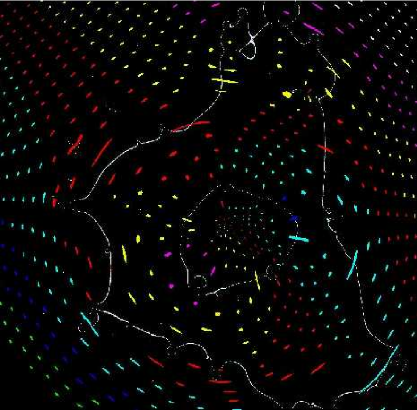
Figure 17: This figure shows the images generated by the best fit lens model of Figure 13, where the sources are colour coded in diagonal stripes across the image, to demonstrate where counter images of the same source may be found. For example, the blue and purple bands of sources form counter images on the opposite side of the radial critical curve, and red coded images form in a ring around the lens including the demagnified region in the center - these correspond to the many 5-image systems identified in Figure 1. Counter images are not expected to form for the outermost images in the field of view.

The location of the radial and tangential critical curves are clearly defined in our data and therefore we examine the constraint they provide on the mass distribution of the lens. The critical curves are obtained from the magnification field of the lens, and readily identified as loci of divergent values, corresponding to positions where images are maximally stretched either tangentially or radially. The radial critical curve is traced by long spoke-like images and by close pairs of images aligned radially and lying on either side of the radial critical curve. Images formed close to this radial ring point towards local concentrations of mass and usually form interior to tangential critical curves. This behaviour is shown in Figures 14,15,&16 , where a grid of evenly spaced circular sources is lensed by our best fitting lens model and projected onto the magnification field to show the relationship between the caustics and the distortion of the lensed images. A colour-coded map shows roughly where images of the same source will be located around the lens, to help develop an intuition for where counter-images (with the same colour) will appear over the surface of the lens and with what orientation and shape to expect (Figure 17).

The magnification at a given position, $\mu(\vec{\theta})$, is given by the Jacobian of the lens mapping (e.g. Young ’81), and may be conveniently expressed in terms of derivatives of the deflection field:

$$\mu(\vec{\theta})^{-1}=1-\nabla\cdot\vec{\alpha}+{d\alpha_{x}\over{dx}}{d\alpha_{y}\over{dy}}-\left[{d\alpha_{x}\over{dy}}\right]^{2}$$ (15)

Hence, the deflection field iterated above in our modeling procedure can be used to generate the magnification field directly. The resulting magnification field is plotted in a series of Figures 14,15&16. The bright lines in this plot correspond to divergences in the mapping following critical curves. The main tangential critical curve forms where the mean interior surface mass density exceeds the critical mass density ($0.95g/cm^{2}$ for A1689 at $z=0.185$, with a source at $z=2$), and is not particularly circular in shape, stretching around a sub-group, and is also perturbed by cluster members. A typical cluster galaxy may have a critical radius of 1-3^′′ and this is added to the large scale deflection of the lens, generating obvious excursions so that the formation of images lying close to the critical curve is strongly influenced by these perturbations.

An inner critical curve is also apparent; this is where images are stretched maximally in the radial direction leading to radial “arcs” pointing towards the cluster center. This is the main radial critical curve and forms if the central mass profile is shallower than isothermal, shrinking to zero radius for a pure isothermal profile (see below). Single radial arcs have been observed in other massive clusters, but here, for the first time, we observe many radial arcs that trace out the entire radial critical curve. We attribute this accomplishment to the unprecedented quality of our data and the powerful magnification of A1689. And we expect that similar high quality images will trace out radial critical curves in other massive clusters as well.

The radial magnification is also of interest below when we examine the azimuthal mass profile and is very simply related to the radial deflection angle:

$$\mu(\theta)^{-1}=\left(1-{\alpha(\theta)\over{\theta}}\right)\left(1-{d\alpha\over{d\theta}}\right)$$ (16)

The first term is the tangential stretch factor and the second is the radial stretch factor. The tangential and radial critical curves are defined by where these terms diverge: at two discrete radii in this azimuthal average. This form for the magnification proves more useful for model comparisons than the 2-D form of Eq. 15, which diverges at many radii due to the asymmetry of the lens.

10.1 Radial vs. Tangential Critical Radii

A striking and simple result follows from comparing the ratio of the Einstein radius, $\simeq 50$ ^′′, to the radius of the radial critical curve, $\simeq 17$^′′, Figure 23). This ratio is $\simeq 3$, close to the minimum value for a power law profile, which we now show tends to the base of natural logs, $e=2.718$ for a flat profile, $p=0$. To see what constraint this ratio places on the inner projected slope of the mass profile, consider a power-law mass distribution. Using equation 3 above for a power-law profile, the tangential $a(\theta)$ and radial $b(\theta)$ stretch factors become:

$$a(\theta)^{-1}={1-{CD\over{2-q}}}\theta^{-q},$$ (17)

and

$$b(\theta)^{-1}=1-CD{{1-q}\over{2-q}}\theta^{-q},$$ (18)

These stretch factors diverge at the tangential critical (Einstein) radius $\theta_{e}$ and at the radial critical radius $\theta_{r}$, so that the ratio of critical radii is simply:

$$\theta_{e}/\theta_{r}=(1-q)^{-1/q},$$ (19)

Hence, the radial critical radius saturates at a maximum value of $\theta_{e}/e$ as $q\rightarrow 0$ and disappears altogether for the isothermal case, as $q\rightarrow 1$. The observed ratio of the critical radii noted above, $\theta_{e}/\theta_{r}\simeq 3$, corresponds to $dlog\Sigma(\theta)/dlog(\theta)\simeq-0.3$, using eqn 19. Clearly then the existence of a well-defined radial critical curve and its large radius relative to the tangential critical curve indicates that the inner mass profile of A1689 is much flatter than the purely isothermal case and will be shown later to compare very well with the more physical models discussed in section 11.5, which are predicted to have shallow central profiles.

11 Mass, Light and Model Profiles

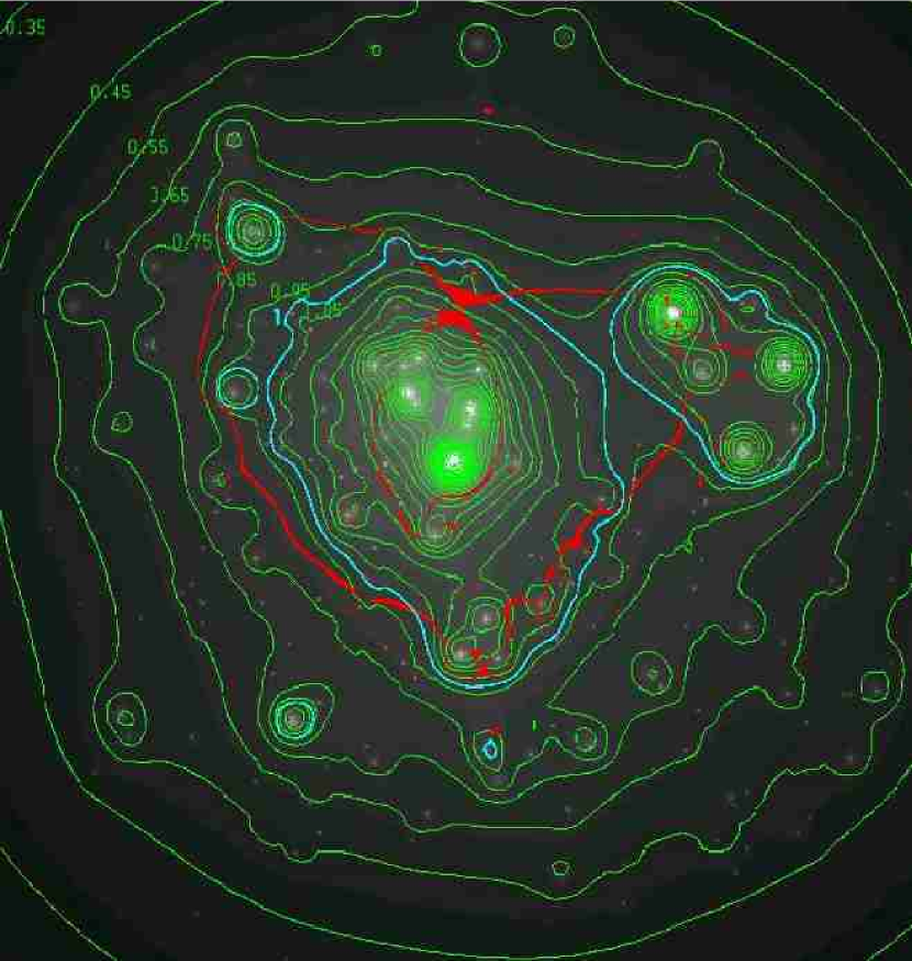
Figure 18: This is the mass distribution before iteration. The double peaked structure reflects the distribution of luminous cluster galaxies used as the starting point for the mass model. The blue contour corresponding to the critical surface density, required to generate multiple images. Other mass contours (green) are labeled in units of this critical density, and the critical curve is overlayed in red.

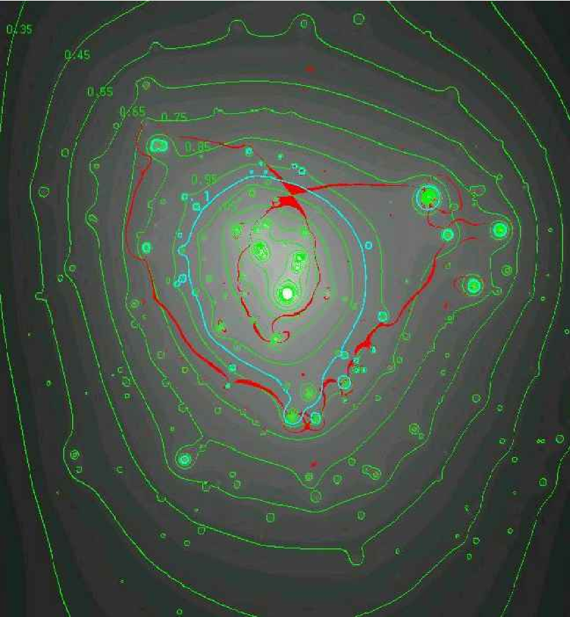
Figure 19: This is the best fitting mass distribution after iteration. Our model is dominated by the main group of central luminous ellipticals, yielding a fairly round mass distribution (rounder than the previous figure) with one main peak centered near (6^′′ from) the most luminous cD galaxy. The main subgroup is found to have much less mass in our model. However, the tangential critical curve (red) is greatly affected by the main subgroup, as image distortions are not linearly related to mass in the strong lensing region but are rather sensitive to perturbations near the Einstein ring. Note that the critical surface mass density contour (blue) is now centered on the main group of galaxies and does not form two “islands” as is the case in the previous figure, for the starting position.

In this section we examine the radial profiles of the mass and light and make comparisons with models. It is necessary to bin the data radially for such comparisons and so we must discuss the role of substructure and ellipticity. The effect of the main subgroup on the mass profile can be seen in the above mass profile (Figures 24,25) as a small flat excess of mass in the mass profile just outside the critical radius. This subgroup is most likely a chance projection lying $\sim 70Mpc/h$ in the background, as argued below. Our model solution down-weights this group as can be seen by comparing the initial mass distribution (Fig. 18) with the model output solution (Fig. 19), where the secondary peak is much less prominent, implying a lower M/L for the subgroup compared with the main cluster. The mass associated with this group can be ignored when determining the radial profile, by excluding a generous area centered on the subgroup. If we exclude a circular area with a radius of 20^′′centered on the four luminous galaxies comprising the subgroup, at a distance of 80^′′ from the center of the cluster, the excess bump in the radial mass profile disappears - Figure 19. Hence the main subgroup has only a minor effect on the mass or light profiles but we can easily exclude it in the subsequent analysis.

11.1 Mass vs. Light

The radial distribution of the mass and light can be compared directly by binning both the model generated mass map and the observed 2D light map of the cluster sequence galaxies. The exact choice of center for constructing radial profiles is not very important. The center of mass must lie close to the center of the radial critical curve, which is approximately circular. This point is nearly coincident with the most luminous central cD galaxy, separated by $\simeq 6$^′′, so that for most purposes we may conveniently use the centroid of the cD galaxy as a representative center for the cluster as a whole. Figure 21 shows a comparison of the mass and light profiles, in circular bins, suitably scaled. The profiles of mass and light are quite similar for $r>50kpc/h$, but with an obvious difference on smaller scales, $r<50kpc/h$. The central luminous galaxies are tightly bunched within this radius, leading to an excess of light over mass, compared with larger radius. One might wonder to what extent the central mass profile is composed of mass associated with these galaxies. We may simply remove the mass associated with the stars in these galaxies by adopting a standard M/L for the luminous regions where velocity dispersion measurements lead to $M/L_{B}\sim 5hM_{\odot}/L_{B}\odot$, (Sheth et al. 2001, Padmanabhan et al. 2002) for luminous elliptical galaxies. If we subtract this mass from the total, the resulting mass profile is offset by a negligible amount over the full range of radius because the M/L of the cluster as a whole is so much larger than that of the starlight, $\sim 400h(M/L_{B})_{\odot}$.

Only if the M/L associated with the galaxies is increased to greater than $30h(M/L_{B})_{\odot}$, is there any significant effect on the profile (Figure 21), producing a slight flattening in the center, $r<20kpc/h$. A large $M/L$ for the galaxies may be reasonable but must include mass well in excess of the baryonic component from the stars and is also in excess of the dynamical masses estimated for luminous elliptical galaxies, $\sim 10(M/L_{B})_{\odot}$. In N-body work, the resulting dark matter profile is not separated into cluster and galaxy components, so for comparison with the N-body work, we include all the mass and do not make any correction for the galaxies. It is not correct to subtract dark matter associated with galaxies when comparing with the N-body work, since this and other substructure is included by default in the N-body based radial mass profiles.

Careful work on other clusters in which the central cD galaxy is much more prominent and the overall M/L of the cluster is lower, so more care is required to evaluate the role of the central galaxy on the strong lensing effects (Sand et al. 2002, Gavazzi et al. 2003, Treu et al. 2003).

It is also worth quoting here an M/L for the region interior to the Einstein radius as this number is usually the only reliable lensing-related quantity for more typical quality data, especially for ground-based data, where one giant arc is often the only strongly lensed image identified. The mass-to-light ratio measured in a circular aperture of 50^′′ centered close to the cD galaxy, is $(M/L)_{Ein}=320\pm 20h(M/L_{B})_{\odot}$, with a small uncertainty as the mean redshift of the critical curve is defined accurately at $\bar{z}=3$ from the average photometric redshift of the multiply imaged background galaxies. This value is identical to that derived for the mass interior to the Einstein ring of CL0024+17, where $M/L(r<100kpc/h)=320\pm 20h(M/L_{B})_{\odot}$ (Broadhurst etal 2000), and corresponds to almost the same physical radius $\sim 100kpc/h$ in projection.

11.2 Radial Magnification Profile

The location of the radial critical curve relative to the tangential critical curve is sensitive to the inner profile of the mass distribution, the ratio of the radii being larger for a shallower profile, as described above. We readily identify the asymmetry of the tangential critical curve which enhances the azimuthally-averaged magnification in circular bins. A corresponding slight excess is seen in the mass profile too but is much less pronounced as the mass distribution is more circularly symmetric than the tangential critical radius (Figure 23). To minimise the effect of the divergent critical lines on the magnification, we can azimuthally average $1/\mu(\vec{\theta})$ over all pixels, and invert this sum to produce a radially binned magnification profile $\mu(r)$. This profile is a much better fit to an NFW profile for the region outside the tangential critical curve, but at the expense of well-defined critical radii.

11.3 Critical Curves and the Light Profile

We can ask where the critical curves should lie if the mass strictly follows the light. By taking the map of the light distribution of galaxies associated with the cluster, described in section 7, and scaling by an average M/L and binned radially we can readily calculate the corresponding magnification profile and identify critical curves. With $M/L\sim 400h(M/L_{B})_{\odot}$, the Einstein radius, although a little noisy, matches the 50^′′ radius observed. However, no obvious radial critical curve is formed. This is because the central light profile is too steep, $\simeq\theta^{-1}$ (close to an isothermal slope) and as pointed out above, equation 19, the radial critical curve shrinks to zero as the index of the profile tends to $p=1$, so that no radial critical curve is expected. Therefore the presence of a large radial critical curve in the data immediately makes clear that the central mass profile is not as steep as that of the light, or equivalently M/L must be lower than average in the center.

Notice that although we began our modeling by taking the light profile as a starting point, the resulting best fit has a shallower mass profile than the light (Figure 21). This, together with the more model-independent conclusion based on the relative ratio of the critical radii (Eqn 19), implies that the mass does not trace the light in detail, and instead the light is more concentrated than the mass. Plausibly, dynamical friction may operate on the cluster galaxies, concentrating them relative to the mass in general, as can be inferred from El-Zant et al. (2003).

11.4 Softened Isothermal Profile

A softened isothermal profile is often discussed as a physical description of a gravitationally relaxed system. Since lensing relates only to the projected mass profile, a distinctive core in 3D will be less obvious in projection. Integrating a softened isothermal potential with a projected core radius of $\theta_{c}$, and Einstein radius, $\theta_{E}$, yields a projected mass profile:

$${\Sigma(\theta)/{\Sigma_{crit}(z)}}={1\over{2}}{{\theta_{c}+\sqrt{\theta_{c}^{2}+\theta_{E}^{2}}}\over{\sqrt{\theta^{2}+\theta_{c}^{2}}}}$$ (20)

Using Eq. 1, the corresponding bend-angle for a softened potential becomes,

$$\alpha(\theta)={1\over{\theta}}(-\theta_{c}+\sqrt{\theta^{2}+\theta_{c}^{2}})(\theta_{c}+\sqrt{\theta_{c}^{2}+\theta_{E}^{2}})$$ (21)

This expression tends to a constant bend-angle of $\alpha=\theta_{E}$ when the core radius is zero, equivalent to the singular isothermal case. For small angles, $\theta<<\theta_{c}$, the bend-angle tends to zero, so that light passing through the core is relatively undeflected by the presence of a core.

If we fix $\theta_{E}$(z=3)=49.5^′′ to match the observations, and vary the core radius, $\theta_{c}$, then a radial critical curve can be generated and matched to the data where $\theta_{r}(z=3)=17$^′′, as shown in Figure 28 (lower right box). The corresponding surface mass profile for this choice of core radius is also shown in Figure 28 (upper right box). This profile is steeper than derived from our observations for angles larger than the core radius, and flattens to a constant density interior to this radius. This profile is not favoured by the observations, although it is surprisingly similar in form, with a mean slope of $d\log\Sigma/d\log(\theta)=-0.8$. The corresponding form of the radial magnification profile is also unlike that derived from the data, being more sharply peaked around $\theta_{E}$ and falls well below predictions for $\theta\leq\theta_{r}$.

We may instead adjust the core radius to match our best fitting mass profile, requiring $\theta_{c}=20$^′′, which produces a significantly larger radius for the radial critical curve, 22^′′, than observed , as shown in Figure 28. This sensitivity to the location of the critical curves is produced by the flattening of the density profile in the core enlarging the radius of the radial critical curve relative to the Einstein radius, so that even a relativity small core has a marked effect on the radius of the radial critical curve.

It is perhaps premature to conclude that the softened isothermal is entirely excluded. More work on the effect of ellipticity and the relative brightness of central images compared with the corresponding counter images at larger radius will allow a fuller exploration of this profile.

The softened isothermal profile is favoured over a generalised NFW profile in the analysis of Gavazzi et al. (2003) for the cD dominated cluster MS1417+22. The authors point out this conclusion hinges on a plausible identification of a faint central image as part of a multiple lensed system and on an accurate description of the central cD galaxy and assumes that the centers of mass of the cD and the cluster mass profile are spatially coincident.

11.5 Comparison with NFW profile

A universal parameterization of CDM-based mass profiles has been advocated by Navarro, Frenk & White (96; NFW hereafter). This is an azimuthally averaged profile summed over sets of haloes identified in N-body simulations and variations between haloes of similar mass are found in detail. This N-body based profile is summed over all the mass contained within the main halo, including the galaxy sized haloes. Hence, we compare our integrated observed mass profile directly with the NFW predictions without having to invent a prescription to remove the cluster galaxies.

NFW have shown that massive CDM haloes are less concentrated with increasing halo mass, a trend identified with collapse redshift, which is generally higher for smaller haloes, following from the increased cosmological density of matter at higher redshift. Cluster haloes, being the most massive bound structures, form later in hierarchical models like CDM, and are therefore have a relatively low concentration, quantified by the ratio of $C_{vir}=r_{virial}/r_{s}$, and found to follow a density profile lacking a core, but with a much shallower central profile ($r\leq 100kpc/h$) than a purely isothermal body. This predicted inner flattening, although a distinctive prediction of CDM-based cosmologies, has not been critically examined by observation for want of discriminating data. Weak lensing measurements, for example, are inherently ambiguous with respect to the mass profile and not able to distinguish the NFW profile from other quite different profiles (e.g. Clowe et al. 2000, King, Clowe & Schneider 2001).

The fit to an NFW profile is made leaving both parameters, $r_{s}$, and $\rho_{s}$ free - the characteristic radius and the corresponding density. These are separately constrained by the critical radii - both the tangential and the radial critical curves and by the form of the projected mass profile. Integrating the mass along a column, z, where $r^{2}=({\xi_{r}}{r_{s}})^{2}+z^{2}$ gives:

$$\rm{M}(\xi_{r})={\rho_{s}}{r_{s}^{3}}(\xi_{r})\int_{o}^{\xi_{r}}d^{2}\xi_{r}\int_{-\infty}^{\infty}{\frac{1}{(r/r_{s})(1+r/r_{s})^{2}}}{dz\over{r_{s}}},$$ (22)

Using this mass, a bend-angle of $\alpha=\frac{4GM(<\theta)}{c^{2}\theta{d_{l}}}\frac{d_{ls}}{d_{s}}$ is produced at position ${\theta}=\xi_{r}{r_{s}}/d_{l}$.

The mean interior mass within some radius $r_{x}=xC_{x}r_{s}$ can be obtained by integration of the NFW profile giving:

$$M(<r)={4\pi\over{3}}r_{x}^{3}{\Omega_{m}(o)\Delta_{c}(1+z)^{3}\over{x^{3}\Omega_{m}(zl)}}{\left[{\log(1+xC_{x})-{xC_{x}\over{1+xC_{x}}}\over{\log(1+C_{x})-{C_{x}\over{1+C_{x}}}}}\right]}$$ (23)

An accurate fit to an NFW profile is achieved with a characteristic radius of $r_{s}=310^{+140}_{-120}kpc/h$ and concentration parameter $C_{vir}=8.2^{+2.1}_{-1.8}$, (figures 25& 27), where the above integral is carried out to the virial radius, $r_{vir}$ (note, sometimes the concentration parameter is quoted for a smaller radius at which the mean interior density is 200 times the cosmological mean density, which gives a smaller value for the concentration parameter, $C_{200}=6.5^{1.9}_{-1.6}$). Note that by incorporating the relative magnifications (section 9) a small improvement in the accuracy of the concentration parameter is obtained (figure 27), $C_{vir}=7.3^{1.6}_{-1.4}$. This corresponds to a virial mass of of $M_{vir}=2.6\times 10^{15}hM_{\odot}$ and a velocity dispersion of $\sigma\sim 1700km/s$ at $r_{s}$ (Figure 31). The fit is remarkable for the way it not only follows the form of the profile all the way to the center of mass, but also accurately reproduces the locations of both the radial and tangential critical curves. One may make a comparison with the entire magnification profile not just the divergent critical radii and this is also shown in Figure 25 (lower left panel). The magnification profile is rather well reproduced overall, with a small excess compared to NFW outside the tangential radius. If we reduce $r_{s}$ to only $100kpc/h$ for example, the critical curves are underestimated by a factor of $\sim 2.5$. This less massive model reproduces the outer weak lensing measurements discussed below but is clearly inconsistent with the strong lensing results.

The concentration parameter derived from this fit is relatively high for such a massive halo. A value of $C_{vir}\sim 5$ is generally anticipated for massive clusters, although the scatter predicted in concentration at a given mass is considerable (eg. Bullock etal 2001). It is important to measure the outer profile of the mass distribution to constrain more clearly the degree of concentration. This we now are tackling with high quality Subaru imaging (Broadhurst etal, in preparation).

12 Weak Lensing, Dynamical, and X-ray Results

We have only sampled the profile to a radius of $250kpc/h$, which corresponds to $r\sim r_{s}$ for the best fit NFW profile obtained above. We may compare the outer profile of A1689 with the weak lensing distortion measurements made by various groups. Weak lensing measurements of A1689 analysed by Clowe & Schneider (2001) and King etal (2002), under-predict the Einstein radius by over a factor of $\sim 2$, predicting an Einstein radius of only 20^′′ compared to the 50^′′  observed and are unable to discriminate significantly between an NFW profile and a purely isothermal profile. The weak lensing signal is known to be heavily diluted in typical ground based data (Kaiser, Squires & Broadhurst 1995), requiring large corrections (a correction factor upward of 3 is typical for the seeing alone) for the seeing and the contamination by undistorted galaxies belonging to the cluster and the foreground. Although this latter effect has been addressed in detail by Clowe & Schneider (2001), they have only one optical passband and thereby suffer maximal contamination. The authors conclude that the mass derived from their weak lensing observations falls well short of the Einstein radius, by a factor $\sim 2.5$, a discrepancy which is reinforced with recent deeper weak lensing work of Bardeau etal 2004 for this cluster using CFHT who find good agreement with the weak lensing measurements of Clowe & Schneider. Tyson & Fischer (1995) on the other hand favour a mass profile which is steeper than isothermal, ($p=-1.4$) for the region $r>100kpc/h$, using modest quality 4m CTIO imaging.

For the small overlap region of the strong lensing and weak lensing data, our best fit model over-predicts the weak lensing strength by $\sim 2.0\pm 0.3$ (Figure 25, bottom right plot). If we take the most concentrated profile consistent with the strong lensing data this discrepancy is reduced by only 30%. Clearly it is important to attempt weak lensing measurements with better seeing and with deep multi-colour images, to minimise the contamination by blue foreground and cluster galaxies.

A redshift survey of the luminous cluster galaxies by Teague, Carter, & Grey (1990), reveals a broad distribution of cluster galaxy velocities and a tail to higher velocities (Figure 31). The large value of $\sigma=2355\pm 200$ km/s derived by Teague, Carter & Grey (1990) is probably overestimated due to the presence of a background sub-group, (Miralda Escudé & Babul 95, Girardi et al. (1997)). Lower values of 1400km/s are preferred by a wavelet analysis of Girardi et al. (1997), though inspection of the 1D distribution of velocities shows that a Gaussian of 1700km/s is a good fit when excluding the only obvious subgroup at +7000km/s (see Figure 31 where we have overlayed this fit). This background group is estimated to have a velocity dispersion of only 700km/s (Girardi et al. 1997) and contains the bright galaxies of the sub-group, which from our strong lensing analysis, is obviously a separate entity distinct from the main body of the cluster. The relatively low velocity dispersion of this sub-group is consistent with our modeling which shows that this group has a noticeably lower M/L compared with the main cluster, by a factor of $\sim 3$.

Xue & Wu (2002) obtained a detailed Chandra X-ray map and limited spectral information for the plasma in A1689. These authors prefer a high gas temperature of $\sim 10-13$KeV, with a trend to somewhat lower temperature towards the center, based on a double beta model fit which aims to account for soft X-ray absorption. The X-ray contours of A1689 are close to circular at all radii, out to $1Mpc/h$, the limit of the data, with no obvious excess corresponding to the main sub-group described above. Naively taking the above gas temperature and assuming the gas and the dark matter are isothermal and that the gas is fully ionized with primordial abundance, then the predicted Einstein radius becomes $\theta_{e}=4\pi(KT/{0.6m_{p}c^{2}})d_{ls}/d_{s}=45$ ^′′, close to the observed value of $\sim 50$ ^′′. More recent X-ray observations of A1689 with XMM (Andersson & Madejski 2004) indicate a maximum temperature of $\sim 8$ KeV, at about the Einstein radius, $100kpc/h$, and the best fit to an NFW profile gives $r_{s}=1.1\pm 0.2Mpc/h$ which is about one third of the value derived here. However, Andersson & Madejski (2004) point out there is evidence of asymmetry of the gas velocity profile and also asymmetry in the temperature map, so that the simple assumption of hydrostatic equilibrium required to derive a cluster mass profile from X-ray temperature and density profile information may not be justified.

13 Cosmological Parameters

In principle, lensing may provide a measurement of the cosmological curvature by simply comparing the scale of the deflection field for multiply lensed sources as a function of source redshift behind a lens. This follows from the simple linear dependence of the bend-angle with the distance ratio, $d_{ls}/d_{s}$, which appears as a scaling term in the general expression for the bend-angle (equation 5). For a given source distance, the deflection field, $\vec{\alpha}(\vec{\theta})$, is proportional to the the distance ratio, $D=d_{ls}/d_{s}$. The bend angles also scale linearly with the amplitude of the surface mass distribution, $\Sigma_{o}$, but this is not measured independently by lensing. Therefore in the absence of any external constraint, the relative scaling of the bend-angle field is proportional to the product of both, $\Sigma_{o}D$. Hence, only the relative scaling of the deflection field can be used when examining cosmological curvature via lensing.

The relative distance ratios of sources lensed by the same cluster are only a weak function of cosmology and are best measured for a given lens using many sources over a wide range of source redshift. In constructing the model mass distribution (section 8) we set the normalisation at a reference redshift of $z=3$, i.e $f_{k}\equiv D(z)/D_{o}$, $D_{o}\equiv D$(z=3). This redshift is preferred as it is the average redshift of the background sources. The function $D(z)$ can be expressed in terms of redshift for a given set of cosmological parameters. In the main case of interest, that of a flat model with a nonzero cosmological constant, the relation is given by:

$$D(z)={c\over H_{0}}\;\frac{1}{(1+z)}\int^{z}_{0}\frac{dz}{[\Omega_{\Lambda}+\Omega_{M}(1+z)^{3}]^{1/2}}$$ (24)

General expressions for the dependence of this distance ratio on arbitrary combinations of $\Omega_{m}$ and $\Omega_{\Lambda}$ are lengthy and can be found in Fukugita et al. (2000).

A comparison of relative deflection angles and hence relative distance ratios has not been feasible to date using strong lensing, as this requires many multiple sources behind a given lens and a reliable model for a statistically meaningful measurement. Here we take our set of models described above and simply determine the value of $f_{k}$ using equation N. Figure 29 (upper panels) shows the values of $f_{k}\equiv D_{k}(z)/D_{o}(z=3)$ for three choices of resulting mass profiles (also shown in Figures 14,15&16) covering the range $0.4<d\log(\Sigma(r)/d\log(r)<1$ and we compare the corresponding predictions for the redshift dependence of $D_{k}(z)/D_{o}(z=3)$, for various choices of cosmological parameters.

The difference between cosmological model for the interesting range $0<\Omega_{M}+\Omega_{\Lambda}\leq 1$ is smaller than the scatter between the data points (Figure 29). However, the form of this function, $D(z)/D_{o}$, does have a distinctive dependence on redshift, virtually independent of the cosmological parameters for the above range. So we may turn the question around and adopt the reasonable assumption that the cosmological parameters lie in the standard range, $0<\Omega_{M}+\Omega_{\Lambda}\leq 1$, and then evaluate the fits to $f_{k}$ to see which profile is preferred. Importantly, this evaluation of the mass profile is independent of our model fitting to the image locations because we do not make use of the redshift information when fitting the model to the locations of the multiple images, since as we showed in section 8.5 (see Figure 12), the output mass distribution is virtually independent of the choice of input values of $f_{k}$ when fitting the image positions.

The values of $f_{k}$ are found to increase with redshift as predicted for the above range of cosmological parameters. In particular, the model resulting in a mean slope of $\bar{p}\simeq 0.55$ (Figure 29, central panel) is preferred by the data over the extreme slopes considered (left and right panels of Figure 29) with a tight scatter about the cosmological relation, accurately following the distinctive trend with redshift.

That the best fitting lens model should produce this sensible geometric trend with redshift adds considerable credibility to the model and need not have turned out so well, as neither the redshift information nor any cosmological model is involved in making the mass model, as noted in section 8.5. Note the scatter on the distance-redshift relation found this way is not small enough to distinguish between the interesting cosmological models, however combinations with $\Omega_{M}+\Omega_{\Lambda}>1.2$ are clearly excluded by the data.

We have evaluated the scatter about the standard cosmological relations as a function of the mean output mass profile finding a smooth trend with a minimum at $\bar{p}\sim 0.55^{+0.1}_{-0.15}$, where the $1\sigma$ scatter is estimated empirically from dispersion on the scatter of the best model $\sigma(D_{i}(z)/D_{o}(z=3))=0.009$. This best fit value for the slope is also the slope preferred by fitting the multiple image positions as described above. Note that the 3 objects with measured redshifts are no better at describing the cosmological redshift dependence than those with photo-z’s, lending, by consistency, further credibility to our method of estimating photometric redshifts in addition to the good agreement with the spectroscopic redshifts.

The lens model can of course be re-run by setting these relative distances to the their best-fit value and rerunning the model to improve the relative distances. However, this iteration produces a negligible change in the mass profile, and only a tiny change in the re-derived relative distances.

With independent mass information for the cluster we may use the lensing information to better discriminate between the models, since the normalization using $D_{o}$(z=3) is not then required. If we take the measured velocity dispersion of the cluster $\sigma=1700\pm 100$ km/s and adopt a circular critical radius based on the pattern of the most tangentially stretched arcs to be approximately $\theta_{e}=40-55$^′′, and we assign the mean redshift of $\bar{z}\sim 3$, we can adjust the amplitude of the mass distribution accordingly, assuming that motions are approximately isothermal, which may not be consistent with the flatter than isothermal mass profile obtained from our modeling. By plotting the unnormalised values of $D_{i}(z)$ compared with the above choices of cosmological parameters, we then see that within the additional uncertainties introduced by the measured velocity dispersion and the uncertain critical radius, little is gained in terms of precision and may be significantly undermined by the assumption of isothermality. Perhaps careful dynamical modeling or hydrodynamic modeling can help to make use of the dynamical and X-ray measurements will help in establishing the benefit of this external information for this cosmological test.

Finally, we mention the benefit of extending this work to higher redshift clusters. For the low redshift of A1689, the distance ratio is close to saturation by $z\sim 1$, so that $d_{s}\simeq d_{ls}$. The dynamic range of $d_{ls}$ can be expanded for higher redshift clusters. For a cluster at z=0.5 for example, the range in $f_{k}$ for source redshifts covering the range $1<z<5$ is 30%, a factor of 3 larger than for A1689 at z=0.185. However, some of this improvement is offset by the naturally smaller critical radius produced for a more distant cluster of fixed mass, as the lens-source separation is smaller and hence the numbers of multiply lensed images will be correspondingly fewer, unless we obtain even deeper images to compensate.

14 Discussion and Conclusions

We have obtained the highest quality images of a lensing cluster to date, surpassing previous work both in terms of depth and spatial resolution and have been rewarded with an order of magnitude increase in the numbers of multiply lensed galaxies identified around an individual cluster. This substantial improvement has permitted detailed modeling of the cluster, which for the first time allows us to trace a radial critical curve and to measure the mass profile of the cluster all the way to the center, inside the radial critical curve, using the many small counter-images found projected on the center of mass.

Also for the first time, we have measured the purely geometric change of the bend-angle with source distance, finding consistency with a flat universe for a wide range of redshift, $1.0<z<5.5$. This is an important consistency check on the currently more accurate measurements of the cosmological parameters at lower redshift, based on SnIa and on the CMB fluctuation spectrum at high redshift.

Our main conclusions are:

• We have identified 106 multiply lensed images, corresponding to 30 multiply lensed galaxies behind A1689. These images include tangential and radially stretched images and also tiny de-magnified central images interior to the radial critical curve. Both the radial and tangential critical curves are delineated in unprecedented detail. This is the first time that any radial critical curve has been traced without a model, just by virtue of the many radial arcs visible. Tiny point-like central images are also found in considerable numbers, allowing for the first time the mass distribution to be traced all the way in to the center of mass.

• The best fitting mass profile derived from the multiple images has a continuously flattening projected slope towards the center of mass with an average gradient of $d\log\Sigma(r)/d\log(r)=-0.55\pm 0.1$, in the observed range of $r<250kpc/h$ and is flatter than the light profile. The profile derived from the positions of the multiple images is checked independently by comparing the relative fluxes of multiple images with the model prediction for the relative magnifications and we also compare the photometric redshift of the multiple images with the relative distances derived from the model. We see that the relative magnifications are reproduced very well by our best fitting model over the full range of radius. The distance-redshift relation is found to follow accurately the form of expected form of the cosmological relation for standard cosmology. These consistencies add considerable confidence that our approach modeling has produced an accurate mass profile for the inner region of A1689.

• The shape of the mass distribution is approximately circular in projection and much rounder than the clumpy spatial distribution of luminous cluster galaxies. In particular the main sub-group is a relatively small mass perturbation. The roundness of this mass distribution argues against this cluster being a lengthly projected filament along the line of sight, though does not rule out a favourable alignment of a triaxial potential boosting the observed surface density.

• A softened isothermal profile can be made to match well the modeled mass profile or to reproduce the locations of the critical radii, but not both simultaneously. The profile is either too steep or has too large a radial critical curve. Nevertheless this model comes strikingly close to matching the data, for a core radius of $\simeq 20$^′′. Given the potential physical importance of any core in the mass distribution, this possibility should be examined more rigorously to evaluate, for example, the influence of ellipticity on the location and shape of the radial critical curve.

• The mass to light ratio of A1689 is high, $M/L(r<250kpc/h)\simeq 400h(M/L_{B})_{\odot}$, 30% larger than any other well-studied cluster, continuing the general trend of higher M/L with increasing mass. This large value means that the stellar mass is a negligible contribution to the overall mass, even in the center $r<50kpc/h$, where the light is more concentrated than the mass. Only for values exceeding $M/L>30h(M/L_{B})_{\odot}$ do galaxies have any noticeable effect on the slope of the inner mass profile. So unlike other lensing work where the cD dominates central mass, we do not suffer from the uncertain subtraction of the central galaxies.

• Our best fitting mass profile to an NFW profile is strikingly good, accounting naturally for the shallow profile observed and its continuous flattening towards the center of mass and the relative radii of the tangential and radial critical curves. This is arguably the most accurate measurement of the central mass profile of any cluster in the region $r<r_{s}$, where the profile of a CDM dominated halo is predicted to be relatively shallow. Interestingly, the concentration parameter we derive for the inner region may be surprisingly high for such a massive halo, and it will be important to examine the form of the mass profile to larger radius with weak lensing measurements to more directly constrain the degree to which the profile as a whole is concentrated.

• The cosmological dependence of the bend-angle of light with redshift scales purely geometrically with the lensing distance ratio, $d_{ls}/d_{s}$. This trend is convincingly detected here, for the first time. It is, however, not a strong function of redshift for the interesting range of cosmological parameters but it is consistent with the standard flat model, and excludes combinations with $\Omega_{M}+\Omega_{\lambda}>1.2$. The agreement need not have been so clear - the modeling does not include the redshift information, so therefore the fact that the bend-angle-redshift trend follows the expected geometric relation add considerable confidence to our approach to lens modeling.

Clearly it is also important to explore the generality of our results by observing other clusters. Our GTO survey will include a few more massive lensing clusters, but the images will be shallower than for A1689, with fewer than 20 orbits each. A more dedicated effort, equivalent in depth to the deep field programs would be very well rewarded, increasing our knowledge of the nature of dark matter, and provide samples of the most distant galaxies and should also permit an independent measurement of the cosmological curvature in a redshift range not covered by SNIa or CMB observations.

Table 1: ACS WFC imaging of ABELL 1689

ACS WFC filter	Exposure time	N exposures	Area (arcmin2)	Extinction	$m_{lim}$	Observation date
F475W	$9500$	$8$	11.73	0.107	27.24	Jun 15th,16th 2002
F625W	$9500$	$8$	11.70	0.076	27.00	Jun 14th 2002
F775W	$11800$	$10$	11.63	0.057	26.92	Jun 13th,20th 2002
F850LP	$16600$	$14$	11.79	0.042	26.50	Jun 12th,16th 2002

Table 2: Multiple arc systems in ABELL 1689

Arc ID	RA (J2000)	Dec (J2000)	X	Y	$i_{F775W}$	$z_{phot}$	$z_{best}$	$z_{spec}$
1.1	13:11:26.4498	-1:19:56.753	8.72	-54.80	23.44	$3.03^{0.53}_{0.53}$	$2.99^{0.48}_{0.48}$	3.04
1.2	13:11:26.2812	-1:20:00.261	4.48	-55.60	23.69	$3.04^{0.53}_{0.53}$	$2.99^{0.48}_{0.48}$	-
1.3	13:11:29.7771	-1:21:07.475	-34.12	20.40	24.52	$3.27^{0.56}_{0.56}$	$2.99^{0.48}_{0.48}$	-
1.4	13:11:33.0629	-1:20:27.403	23.08	48.00	24.16	$2.94^{0.52}_{0.52}$	$2.99^{0.48}_{0.48}$	3.05
1.5	13:11:31.9350	-1:20:05.998	35.27	23.60	24.62	$3.35^{0.57}_{0.57}$	$2.99^{0.48}_{0.48}$	-
1.6	13:11:29.8536	-1:20:38.413	-7.33	9.10	25.82	$1.06^{1.91}_{0.27}$	$2.99^{0.48}_{0.48}$	-
2.1	13:11:26.5237	-1:19:55.450	10.38	-54.35	23.37	$2.62^{0.47}_{0.48}$	$2.54^{0.42}_{0.42}$	-
2.2	13:11:32.9642	-1:20:25.494	24.18	45.85	24.18	$2.57^{0.47}_{0.47}$	$2.54^{0.42}_{0.42}$	-
2.3	13:11:31.9728	-1:20:07.147	34.48	24.60	24.36	$2.64^{0.48}_{0.48}$	$2.54^{0.42}_{0.42}$	-
2.4	13:11:29.8119	-1:21:06.008	-32.58	20.25	24.48	$2.36^{0.44}_{0.44}$	$2.54^{0.42}_{0.42}$	-
2.5	13:11:29.8790	-1:20:39.365	-8.03	9.85	25.63	$1.59^{0.86}_{0.34}$	$2.54^{0.42}_{0.42}$	-
3.1	13:11:32.0428	-1:20:27.520	16.48	34.20	26.65	$5.48^{0.85}_{0.85}$	$5.47^{0.78}_{0.78}$	-
3.2	13:11:32.1718	-1:20:33.287	12.08	38.40	26.85	$5.45^{0.85}_{0.85}$	$5.47^{0.78}_{0.78}$	-
3.3	13:11:31.6850	-1:20:56.040	-11.62	41.45	-	-	$5.47^{0.78}_{0.78}$	-
4.1	13:11:32.1705	-1:20:57.355	-9.73	48.60	24.62	$1.06^{0.27}_{0.27}$	$1.33^{0.28}_{0.28}$	-
4.2	13:11:30.5186	-1:21:12.026	-33.52	32.40	23.91	$1.32^{0.30}_{0.31}$	$1.33^{0.28}_{0.28}$	-
4.3	13:11:30.7576	-1:20:08.322	25.68	8.60	25.12	$1.47^{0.32}_{0.33}$	$1.33^{0.28}_{0.28}$	-
4.4	13:11:26.2866	-1:20:35.422	-27.33	-40.60	24.67	$1.33^{0.31}_{0.31}$	$1.33^{0.28}_{0.28}$	-
4.5	13:11:29.8458	-1:20:29.357	0.83	5.15	-	-	$1.33^{0.28}_{0.28}$	-
5.1	13:11:29.0655	-1:20:48.776	-21.73	2.80	24.42	$3.29^{0.56}_{0.56}$	$3.27^{0.51}_{0.51}$	-
5.2	13:11:29.2248	-1:20:44.153	-16.53	3.00	24.92	$3.16^{0.55}_{0.55}$	$3.27^{0.51}_{0.51}$	-
5.3	13:11:34.1199	-1:20:20.919	35.68	59.60	25.26	$2.15^{0.67}_{0.41}$	$3.27^{0.51}_{0.51}$	-
6.1	13:11:30.7484	-1:19:37.995	53.08	-4.40	23.61	$1.22^{0.29}_{0.29}$	$1.17^{0.26}_{0.26}$	-
6.2	13:11:33.3475	-1:20:12.174	38.68	45.40	23.85	$1.31^{0.30}_{0.30}$	$1.17^{0.26}_{0.26}$	-
6.3	13:11:32.7510	-1:19:54.506	50.88	29.80	23.02	$0.94^{0.26}_{0.25}$	$1.17^{0.26}_{0.26}$	-
6.4	13:11:32.4824	-1:19:58.857	45.23	28.00	24.00	$1.09^{0.27}_{0.27}$	$1.17^{0.26}_{0.26}$	-
7.1	13:11:25.4491	-1:20:51.843	-47.53	-45.00	23.31	$4.92^{0.78}_{0.78}$	$4.92^{0.71}_{0.71}$	4.87
7.2	13:11:30.6715	-1:20:13.902	20.08	9.80	24.19	$5.20^{0.81}_{0.81}$	$4.92^{0.71}_{0.71}$	-
7.3	13:11:29.8204	-1:20:24.870	4.73	2.90	28.23	$0.77^{4.01}_{0.23}$	$4.92^{0.71}_{0.71}$	-
8.1	13:11:32.2984	-1:20:50.909	-3.08	47.60	24.54	$2.63^{0.48}_{0.48}$	$2.67^{0.48}_{0.74}$	-
8.2	13:11:31.4027	-1:21:05.541	-22.03	41.65	24.31	$2.77^{0.50}_{0.50}$	$2.67^{0.48}_{0.74}$	-
8.3	13:11:31.5056	-1:20:14.078	25.23	21.20	25.71	$2.75^{0.49}_{0.89}$	$2.67^{0.48}_{0.74}$	-
8.4	13:11:25.5301	-1:20:20.162	-18.32	-57.35	23.97	$0.70^{0.22}_{0.22}$	$2.67^{0.48}_{0.74}$	-
8.5	13:11:30.3295	-1:20:30.494	2.88	12.20	27.42	$0.77^{2.53}_{0.23}$	$2.67^{0.48}_{0.74}$	-
9.1	13:11:30.3084	-1:19:48.652	40.62	-5.85	25.92	$4.97^{0.78}_{0.78}$	$5.16^{0.74}_{0.74}$	-
9.2	13:11:33.5206	-1:20:50.335	5.23	63.95	27.53	$1.06^{0.27}_{0.27}$	$5.16^{0.74}_{0.74}$	-
9.3	13:11:28.7470	-1:21:15.805	-48.23	9.95	25.72	$5.16^{0.81}_{0.81}$	$5.16^{0.74}_{0.74}$	-
9.4	13:11:26.2723	-1:20:26.927	-19.73	-44.40	27.15	$5.17^{0.81}_{0.81}$	$5.16^{0.74}_{0.74}$	-
10.1	13:11:33.9794	-1:20:50.855	7.68	70.40	23.66	$1.75^{0.74}_{0.36}$	$1.57^{0.31}_{0.31}$	1.37
10.2	13:11:28.0499	-1:20:12.477	4.67	-26.40	23.30	$1.54^{0.33}_{0.33}$	$1.57^{0.31}_{0.31}$	-
10.3	13:11:29.3180	-1:20:27.744	-1.07	-2.70	25.15	$2.57^{0.47}_{0.63}$	$1.57^{0.31}_{0.31}$	-
11.1	13:11:33.3423	-1:21:06.754	-10.78	68.50	24.03	$2.91^{0.51}_{0.51}$	$2.90^{0.47}_{0.47}$	-
11.2	13:11:29.0588	-1:20:01.292	21.23	-17.45	23.36	$2.87^{0.51}_{0.51}$	$2.90^{0.47}_{0.47}$	-
11.3	13:11:29.4933	-1:20:26.381	1.28	-0.90	26.78	$1.58^{0.73}_{0.52}$	$2.90^{0.47}_{0.47}$	-
12.1	13:11:30.3638	-1:19:51.471	38.43	-3.90	25.39	$1.87^{0.38}_{0.38}$	$1.87^{0.34}_{0.34}$	1.82
12.2	13:11:27.3591	-1:20:54.946	-38.18	-17.75	24.30	$1.99^{0.39}_{0.39}$	$1.87^{0.34}_{0.34}$	1.82
12.3	13:11:27.2257	-1:20:51.910	-36.27	-20.85	23.97	$1.99^{0.39}_{0.39}$	$1.87^{0.34}_{0.34}$	-
12.4	13:11:28.9644	-1:21:10.265	-41.83	10.55	25.93	$1.92^{0.38}_{0.38}$	$1.87^{0.34}_{0.34}$	-
12.5	13:11:33.4898	-1:20:51.555	3.93	64.05	25.55	$1.87^{0.38}_{0.38}$	$1.87^{0.34}_{0.34}$	-
13.1	13:11:32.8241	-1:19:24.371	78.62	18.00	24.10	$1.02^{0.28}_{0.27}$	$1.02^{0.24}_{0.24}$	-
13.2	13:11:32.9847	-1:19:25.831	78.33	20.80	23.68	$0.72^{0.23}_{0.23}$	$1.02^{0.24}_{0.24}$	-
13.3	13:11:33.3934	-1:19:31.134	76.12	28.60	24.12	$1.10^{0.28}_{0.28}$	$1.02^{0.24}_{0.24}$	-
14.1	13:11:29.0279	-1:21:41.802	-69.98	24.80	24.98	$3.37^{0.57}_{0.82}$	$3.41^{0.53}_{0.53}$	-
14.2	13:11:29.4588	-1:21:42.623	-67.98	31.00	25.99	$3.64^{0.61}_{0.61}$	$3.41^{0.53}_{0.53}$	-
15.1	13:11:28.0753	-1:20:15.196	2.38	-24.90	25.69	$1.99^{0.39}_{0.39}$	$1.99^{0.36}_{0.36}$	-
15.2	13:11:34.0756	-1:20:51.311	7.88	71.90	25.79	$2.00^{0.39}_{0.39}$	$1.99^{0.36}_{0.36}$	-
15.3	13:11:29.2387	-1:20:27.573	-1.43	-3.85	27.16	$1.97^{0.39}_{0.43}$	$1.99^{0.36}_{0.36}$	-
16.1	13:11:27.9835	-1:20:25.319	-7.38	-21.85	23.68	$1.81^{0.37}_{0.37}$	$2.01^{0.36}_{0.36}$	-
16.2	13:11:28.9137	-1:20:28.546	-4.38	-7.85	25.06	$2.26^{0.43}_{0.43}$	$2.01^{0.36}_{0.36}$	-
16.3	13:11:34.3985	-1:20:46.402	14.38	74.20	25.35	$1.80^{0.71}_{0.37}$	$2.01^{0.36}_{0.36}$	-
17.1	13:11:30.6557	-1:20:24.890	10.03	14.25	24.19	$2.74^{0.49}_{0.49}$	$2.22^{0.39}_{0.39}$	-
17.2	13:11:30.3890	-1:20:27.765	5.73	11.85	25.11	$2.02^{0.40}_{0.40}$	$2.22^{0.39}_{0.39}$	-
17.3	13:11:24.9804	-1:20:41.865	-41.48	-55.60	24.31	$2.25^{0.43}_{0.43}$	$2.22^{0.39}_{0.39}$	-
18.1	13:11:28.2448	-1:20:09.540	8.58	-25.00	25.00	$2.56^{0.47}_{0.47}$	$2.54^{0.42}_{0.42}$	-
18.2	13:11:33.8200	-1:20:54.539	3.33	69.80	-	-	$2.54^{0.42}_{0.42}$	-
18.3	13:11:29.3622	-1:20:27.392	-0.48	-2.25	26.78	$1.58^{0.73}_{0.52}$	$2.54^{0.42}_{0.42}$	-
19.1	13:11:31.6333	-1:20:22.597	18.32	26.55	24.83	$1.72^{0.36}_{0.36}$	$2.63^{0.44}_{0.44}$	-
19.2	13:11:25.2404	-1:20:20.003	-20.03	-61.35	25.23	$2.74^{0.49}_{0.49}$	$2.63^{0.44}_{0.44}$	-
19.3	13:11:31.9546	-1:20:59.315	-12.88	46.50	25.88	$1.57^{0.34}_{0.34}$	$2.63^{0.44}_{0.44}$	-
19.4	13:11:32.0523	-1:20:57.131	-10.28	46.90	24.76	$2.58^{0.47}_{0.47}$	$2.63^{0.44}_{0.44}$	-
19.5	13:11:30.2100	-1:20:33.961	-1.03	12.05	27.94	$4.54^{1.66}_{0.73}$	$2.63^{0.44}_{0.44}$	-
20.1	13:11:31.1430	-1:21:40.935	-55.73	53.15	22.80	$1.63^{0.35}_{0.34}$	$1.12^{0.25}_{0.25}$	-
20.2	13:11:32.2212	-1:21:29.299	-38.33	62.85	-	-	$1.12^{0.25}_{0.25}$	-
21.1	13:11:31.0264	-1:20:45.776	-6.53	28.15	25.15	$1.79^{0.37}_{0.37}$	$1.78^{0.33}_{0.33}$	-
21.2	13:11:30.8009	-1:20:44.743	-7.03	24.65	26.70	$1.59^{0.34}_{0.34}$	$1.78^{0.33}_{0.33}$	-
21.3	13:11:25.2540	-1:20:11.207	-11.98	-64.90	25.59	$1.78^{0.36}_{0.36}$	$1.78^{0.33}_{0.33}$	-
22.1	13:11:29.6859	-1:20:08.794	18.43	-5.75	23.66	$1.99^{0.39}_{0.39}$	$1.98^{0.36}_{0.36}$	-
22.2	13:11:29.6156	-1:20:23.762	4.42	-0.35	25.49	$1.99^{0.59}_{0.39}$	$1.98^{0.36}_{0.36}$	-
22.3	13:11:32.4150	-1:21:15.917	-24.98	59.80	23.27	$1.96^{0.39}_{0.39}$	$1.98^{0.36}_{0.36}$	-
23.1	13:11:29.5299	-1:20:10.016	16.32	-7.35	24.63	$2.03^{0.40}_{0.40}$	$2.00^{0.36}_{0.36}$	-
23.2	13:11:29.5545	-1:20:22.891	4.83	-1.55	25.99	$1.99^{0.62}_{0.39}$	$2.00^{0.36}_{0.36}$	-
23.3	13:11:32.6585	-1:21:15.199	-22.78	62.80	24.72	$2.00^{0.39}_{0.39}$	$2.00^{0.36}_{0.36}$	-
24.1	13:11:29.1913	-1:20:56.177	-27.62	7.65	25.24	$2.63^{0.48}_{0.48}$	$2.52^{0.42}_{0.42}$	-
24.2	13:11:32.0642	-1:19:50.560	50.08	18.80	24.80	$2.50^{0.46}_{0.46}$	$2.52^{0.42}_{0.42}$	-
24.3	13:11:30.2944	-1:19:34.140	53.68	-12.20	24.33	$2.43^{0.45}_{0.45}$	$2.52^{0.42}_{0.42}$	-
24.4	13:11:33.7184	-1:20:19.863	34.08	53.70	24.99	$2.81^{0.50}_{0.69}$	$2.52^{0.42}_{0.42}$	-
24.5	13:11:29.6289	-1:20:36.999	-7.48	5.45	27.27	$4.55^{0.80}_{0.73}$	$2.52^{0.42}_{0.42}$	-
25.1	13:11:28.4949	-1:20:34.990	-12.88	-10.80	25.44	$4.59^{0.73}_{0.73}$	$4.53^{0.66}_{0.66}$	-
25.2	13:11:34.6484	-1:20:33.581	27.58	72.15	26.62	$4.42^{0.71}_{0.71}$	$4.53^{0.66}_{0.66}$	-
26.1	13:11:25.1545	-1:20:32.763	-32.12	-57.10	24.67	$1.08^{0.39}_{0.27}$	$1.07^{0.25}_{0.25}$	-
26.2	13:11:31.3260	-1:20:25.241	13.98	23.50	25.39	$1.04^{0.27}_{0.27}$	$1.07^{0.25}_{0.25}$	-
26.3	13:11:30.2420	-1:20:32.585	0.43	11.90	27.42	$0.77^{2.53}_{0.23}$	$1.07^{0.25}_{0.25}$	-
27.1	13:11:25.1730	-1:20:33.113	-32.33	-56.70	25.22	$1.81^{0.37}_{0.37}$	$1.74^{0.33}_{0.33}$	-
27.2	13:11:31.3668	-1:20:24.644	14.78	23.80	26.19	$1.58^{0.48}_{0.34}$	$1.74^{0.33}_{0.33}$	-
27.3	13:11:30.1918	-1:20:32.894	-0.18	11.35	29.82	$4.55^{1.63}_{0.73}$	$1.74^{0.33}_{0.33}$	-
28.1	13:11:28.2978	-1:20:10.907	7.68	-23.70	27.20	$1.17^{4.29}_{0.29}$	$5.45^{0.77}_{0.77}$	-
28.2	13:11:34.2602	-1:21:00.009	1.18	78.10	26.47	$2.00^{0.43}_{1.23}$	$5.45^{0.77}_{0.77}$	-
29.1	13:11:29.2256	-1:20:57.909	-28.98	8.85	25.97	$2.47^{0.57}_{0.46}$	$2.49^{0.42}_{0.42}$	-
29.2	13:11:30.0380	-1:19:34.215	51.98	-15.65	25.00	$3.40^{0.58}_{0.58}$	$2.49^{0.42}_{0.42}$	-
29.3	13:11:32.1451	-1:19:52.565	48.78	20.75	24.80	$2.50^{0.46}_{0.46}$	$2.49^{0.42}_{0.42}$	-
29.4	13:11:33.6261	-1:20:20.815	32.62	52.85	25.84	$3.35^{0.57}_{0.57}$	$2.49^{0.42}_{0.42}$	-
29.5	13:11:29.7297	-1:20:36.603	-6.48	6.65	27.97	$4.59^{1.66}_{0.73}$	$2.49^{0.42}_{0.42}$	-
30.1	13:11:32.4212	-1:19:19.826	80.18	10.60	25.91	$4.49^{0.72}_{0.72}$	$3.28^{0.51}_{0.51}$	-
30.2	13:11:33.1835	-1:19:26.069	79.38	23.60	25.80	$3.23^{0.56}_{0.76}$	$3.28^{0.51}_{0.51}$	-
30.3	13:11:33.6540	-1:19:32.691	76.38	32.80	25.73	$3.30^{0.56}_{0.56}$	$3.28^{0.51}_{0.51}$	-

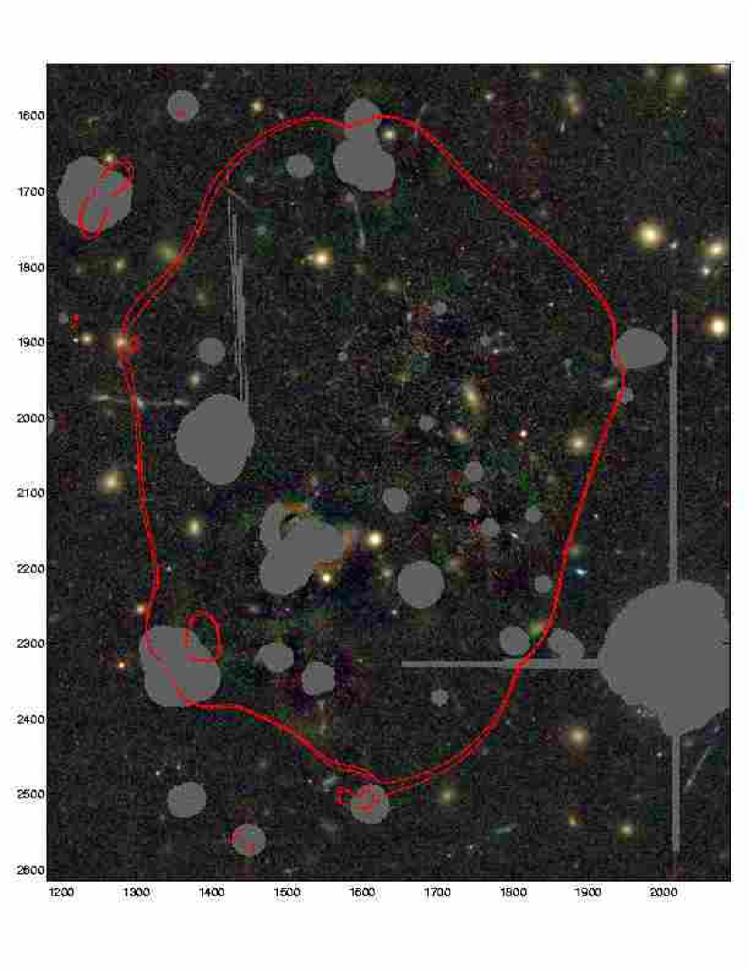
Figure 6: A blow-up of the central region with the bright elliptical galaxies subtracted. Significant residuals are masked out, as are stars and image artifacts. Overlaid is the model radial critical curve for $z_{s}=3$ ($f_{k}\equiv 1$). Several highly elongated spoke-like images can be seen close to this curve, in some cases bisecting the critical curve. Other images close to the curve generally point in a radial direction towards the center of mass (in the middle of the radial critical curve), and others are split on either side.

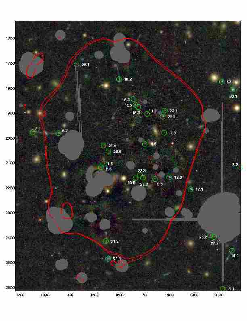
Figure 7: Blow-up of the central region with the bright elliptical galaxies subtracted with the counter-images marked with their ID corresponding to Table 2. These images are either long and point radially or are small images interior to the radial critical curve, some of which are demagnified and seen here for the first time in appreciable numbers. Such central images are very helpful in constraining the inner mass profile.

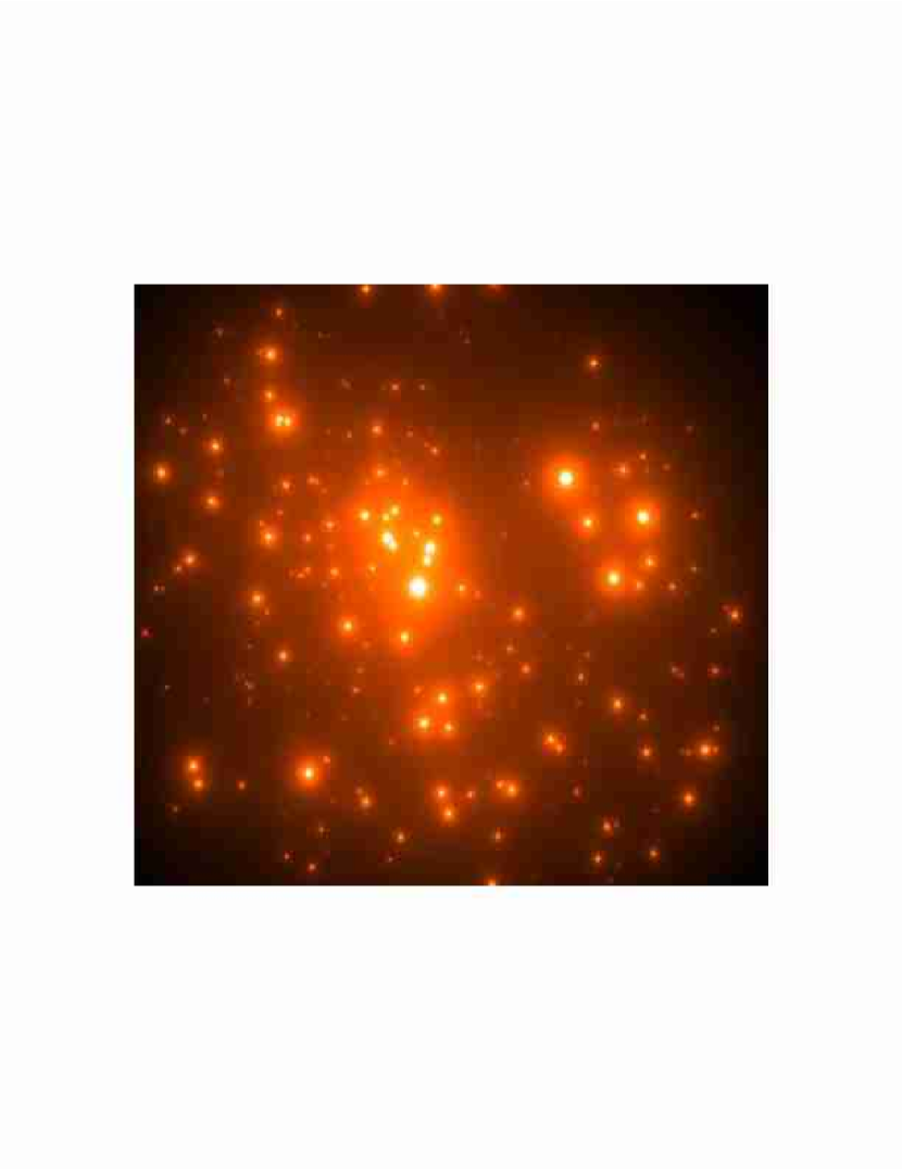
Figure 9: This is the starting point for our lens model. A plausible projected surface density map is constructed by summing up profiles assigned to all cluster sequence galaxies. Each galaxy is modeled simply as an extended power-law density profile (in this figure $q=1$) with a normalization proportional to luminosity. The result is a surface density map which scales linearly with $M/L$, and has an overall smooth appearance, punctuated by galaxy peaks.

Figure 10: A low order cubic-spline fit to the surface mass density in the previous figure produces a smooth component. After calculating its corresponding deflection field, we will add low order perturbations in order to produce a smooth deflection field for fitting the multiple-image locations. The main departure from circularity visible on the left follows a the most luminous sub-group of galaxies.

Figure 11: A “lumpy” residual map is formed by subtracting the previous smooth component from the initial surface mass distribution. This map highlights the galaxies, and we use it to crudely represent them as concentrations of mass with the correct locations. More accurate descriptions of galaxies are not justified in the context of cluster lensing as the galaxy contribution is very small and only important for cases where a multiply lensed image falls near a massive galaxy. Our modeling allows only the amplitude of deflection field corresponding to this map to vary with respect to the smooth component; this approximates varying M/L of the galaxy component relative to the cluster component.

Figure 12: The left-hand panel shows the random values of the relative distance ratio,$f_{k}$, which we input to test the modeling procedure. $f_{k}$ is plotted against redshift, showing no inherent trend. On the right are the output values of $f_{k}$ from the model, which are found to follow a tight relation with redshift. A constant input value of $f_{k}$ (open circles) is used in our modeling to avoid specifying many additional free parameters, and can be seen to behave in the same way with redshift as the random input. The relative deflection angles scale in a way which is redshift-dependent with a small scatter in $f_{k}$ that varies between sources slightly, depending on the the location of the multiple images of each source. This redshift dependence is compared to the expected behaviour of cosmological models (Section 13).

Figure 13: The relative distance ratios, $f_{k}$ for 28 multiply-lensed galaxies with redshift measurements or reliable photo-z’s. The left-hand plot shows the calculated value for each set of images before the model is iterated using the input mass distribution, and the right-hand shows the marked improvement achieved when the iteration procedure is applied to minimise the overall error on the model image positions, described in section 8.3. The bend-angle is scaled to $z=3$ ($f_{k}\equiv 1$). The absolute bend-angles are not known independently as they are products of the relative distances and the normalization of the mass map. The three close curves cover the range of currently interesting cosmologies, which in order of increasing gradient are ($\Omega_{m},\Omega_{\lambda}$) = (0.1, 0), (0.3, 0.7), (1, 0), and (0.1, 1.2), this final (upper) curve being discrepant. This plot demonstrates that the bend-angles predicted by the model are fully consistent with the purely geometric effect expected for any reasonable cosmology. Higher redshift clusters must be examined in order to constrain the cosmological parameters with more accuracy. Note that two very close pairs of images (sources 13 & 14) are excluded from this plot as their predicted locations are too sensitive to the location of the critical curve which in both cases passes between producing an unreliable distance estimate. The remarkable point here is that the redshift information is not used in generating the best fit model - only the angular information on the image locations, and hence the sensible trend found here of bend-angle vs. redshift adds considerable confidence regarding the model.

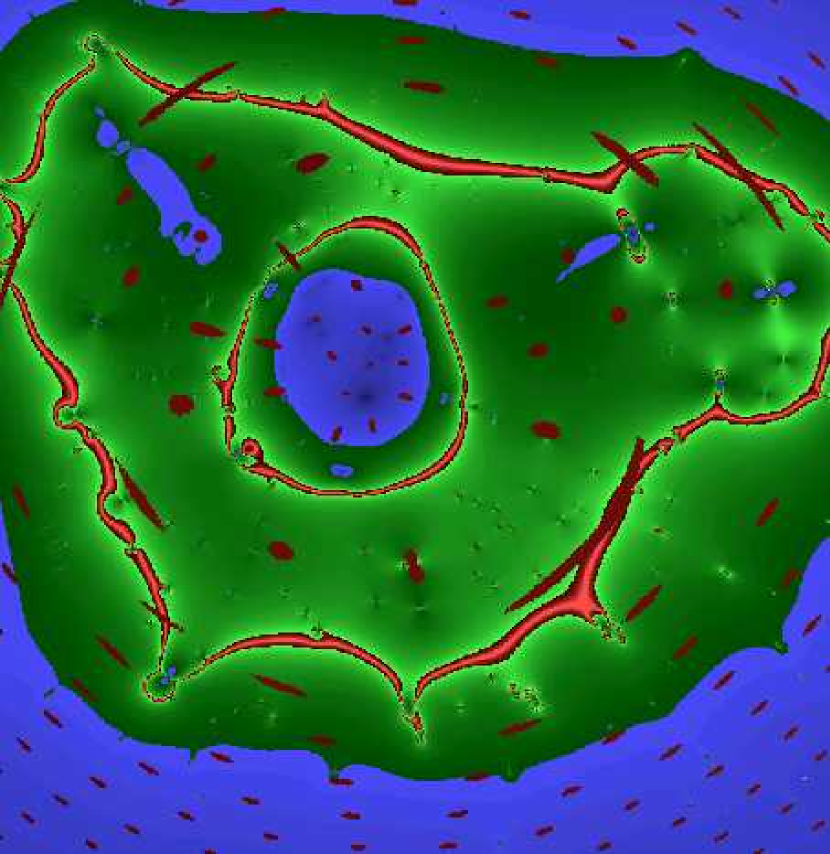
Figure 16: The profile here is relatively shallow, corresponding to the profile in the left-hand column of Figure 31. A larger radial critical curve forms and the relative magnification of images interior to the radial critical curve are larger than for steeper profiles, and the arcs are relatively longer.

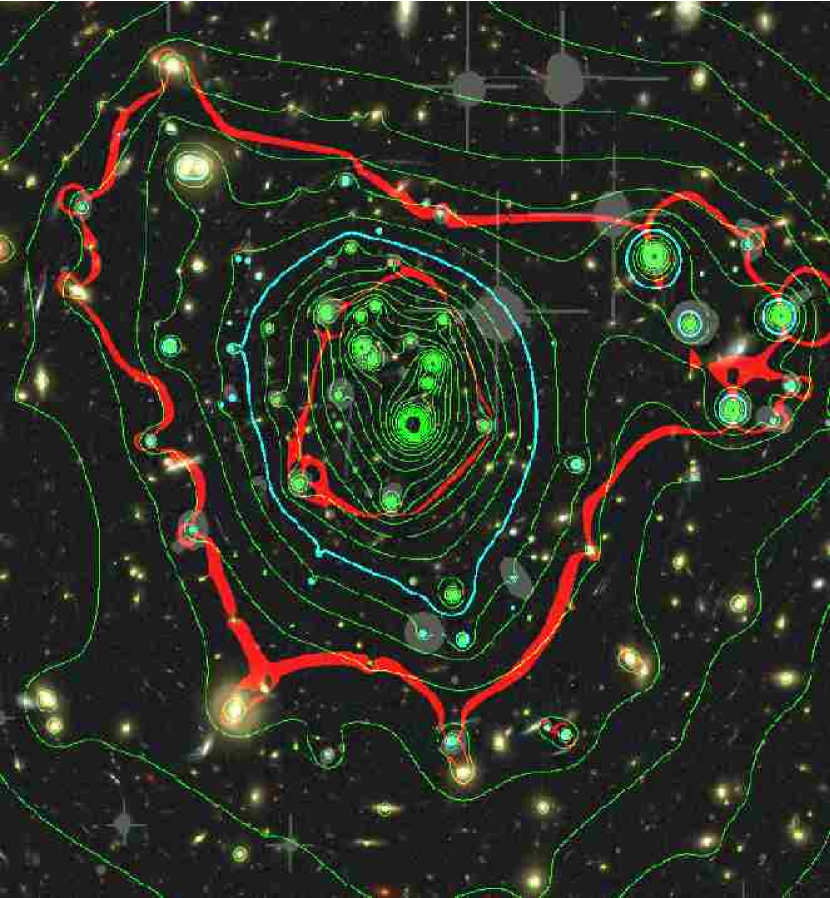
Figure 20: The resulting mass distribution and critical curves (scaled to $z=3$ ($f_{k}\equiv 1$)) are plotted on the colour image of the arcs - with the cluster galaxies removed, showing the relation between the shape of the lensed images and the model. Note how the giant arc is exactly bisected by the critical curve forming two large mirror images (images 8.1 & 8.2).

Figure 21: The mass and light profiles are compared in the left-hand panel for our best fit model. The light profile (dashed curve with circular points attached) is more concentrated than the mass (solid lines). Four curves (solid) are shown for the mass distribution, which differ in the amount of mass assigned to the galaxies and subtracted from the total. This subtraction is performed in 2D using the light map described in the text. The upper mass curve is the total mass, and the three slightly lower curves have mass subtracted by scaling the radial light curve (dished line) by the ratio $M/L=5,10\&30h(M/L_{B})_{\odot}$. This has negligible effect, even in the center where the light peaks, due to the very high M/L of the cluster as a whole. Excluding the light of the subgroup from the overall light profile is shown too (small dashes) and this has a small effect on the light profile, in particular it raises the overall $M/L$ (right hand panel - dashed curve).

Figure 22: This shows the range of acceptable profiles corresponding to the 1$\sigma$ limits on fitting the image locations. The corresponding range of $M/L$ profiles is plotted in the right-hand panels - the steeper slope has the lower overall M/L at large radius. Note that profiles of differing slopes must cross within the Einstein radius, as can be seen in the left-hand panel, as the total mass is fixed by definition for a given observed Einstein radius, and is independent of the mass profile.

Figure 23: The radial magnification profile for the data determined from the 2D map diverges over a wide range of radius because the tangential critical curve is not circular but has excursions around sub-groups. So to help better define critical curves we average $1/\mu(r)$, and plot the inverse of this - solid curve and now the the radial and tangential critical radii are well defined. If instead we calculate the magnification profile form the radially average mass distribution (using equation 16) then the profile is is better behaved, diverging at only two points - dashed curve, and the radii of these divergent points corresponds well the the maxima of the solid curve calculated from the 2D map. In the next series of figures we make radial comparisons of theoretical predictions with the latter curve, derived by using the radially binned mass maps.

Figure 24: Comparison of the best fit model profile (upper left panel) with the NFW prediction of CDM - shown is $r_{s}=310kpc/h$, $C=8.2$. The dashed line is the singular isothermal case normalised to the observed Einstein radius for comparison. The scale is linear in angle, to help show the accuracy of the fit. The full logarithmic form is shown top right compared with the full NFW profile demonstrating that our lensing data covers only the shallow region of the profile interior to $r<r_{s}$. The bottom left panel is the magnification derived by our best-fitting model, compared with the NFW prediction, demonstrating how well the locations of the critical curves are reproduced at radii of $\sim 17$^′′ and $\sim 50$^′′ by the NFW model, and also that the central magnification is accurately followed. There is a slight excess outside the tangential critical radius which results from the elongated shape of the tangential critical curve, enhancing the azimuthally averaged magnification in circular bins. A much smaller excess can be seen in the radial mass profile, which is less pronounced because the mass distribution is inherently rounder than the path of the tangential critical curve (see Figure 14 for a 2D comparison of mass contour with the path of the tangential critical curve). The weak lensing measurements of Clowe & Schneider are shown (bottom right panel) versus the ellipticity expected for the best fitting NFW profile. The weak lensing data imply a much smaller tangential critical radius than observed (20^′′ vs 50^′′) indicating some problem.

Figure 25: This is the same as the previous figure but with the main subgroup excluded (see text) when making all azimuthally averaged profiles. The fit to the NFW profile is very good, though the concentration parameter, $C_{vir}=8.2$, is somewhat larger than predicted for cluster mass haloes.

Figure 26: The left-hand panels show a shallow surface density profile and the magnification for a shallow profile case corresponding to 2D map of figure 16, and which poorly fits the multiple image positions. The radial critical curve is too large and the magnifications are enormous. The right-hand panels show a profile which is steep to match well the multiple image locations, and can be seen to have only a very small radial critical curve. These profiles correspond to the 2D map shown in figure 15.

Figure 27: Chi-squared contours of the NFW profile fit for the characteristic radius, $r_{s}$ and the concentration parameter, $C=r_{vir}/r_{s}$. The best fit value is marked at $C=8.2$ and $r_{s}=310kpc/h$. The contours correspond to 1, 2 &3 $\sigma$ and are calculated using the dispersion about the best fit model, shown in Figure 22. The dashed set of contours show the fit when the relative magnifications of the lensed images are included.

Figure 28: The solid curves are for a softened isothermal profile, compared with the best fit solution for the mass profile and magnification profile. The upper left-hand box shows that the mass profile is well fitted by the model profile with a core radius of 22^′′. However, the corresponding radius of the radial critical curve significantly exceeds the observed radius - lower left box. If instead the core radius of the softened isothermal model is reduced to 11^′′ to reproduce the observed radius of the radial critical curve - lower right box - then the slope of the projected profile is too steep to match the lens model - upper right box.

Figure 29: Three model outputs are shown for differing mass profiles - from shallow to steep (bottom left to right panels) corresponding to figures 14,15&16. The upper panel (left to right) shows the corresponding values of the relative distance ratio’s ,$f_{k}$, for these three choices of profile. The best fit to the cosmological curvature is for the central case, $p\simeq-0.55$, where the relative bend angles follow smoothly the expected cosmological behaviour and are consistent with a flat universe (see also figure 13 right-hand panel). The flatter profile generates a shallower trend with redshift and the steeper profile does the opposite - the derived relation is steeper. The central panel shows the relative image magnifications, which again favour the model which best-fits the multiple image positions, (center) with minimal dispersion and a mean value of unity.

Figure 30: Here we compare errors for differing output model profiles, which we charactersise for simplicity by the mean output slope, $p=d\log\Sigma/d\log r$ average over the observed range of radius. The left-hand plot shows the difference between the model image positions vs. the observed image positions, as a function of the profile slope. There is clearly a pronounced minimum for $p\sim 0.55$ with an average positional error of 3^′′(this is the model we have referred to throughout as our best fit). The central panel shows the error on fit to the standard $\Omega_{m}=0.3+\Omega_{\lambda}=0.7$ cosmology with a similar minimum using the predicted photo-z’s and relative distance ratios, $f_{k}$ (see upper panel of previous figure). The right-hand panel is the dispersion of the relative magnifications about the model (see middle panel of previous figure). The data is most similar to the model for $p\sim 0.5-0.6$, where it has a value consistent with unity and minimal dispersion. These three estimates are largely independent and are in good agreement. Since only the image locations were used in deriving the model fits - the photo-z’s used in the central plot and the fluxes used in the right hand plot provide independent information for constraining the model. The excellent agreement adds considerable weight to our approach to modeling.

Figure 31: Redshift histogram for galaxies in field of A1689. The solid curve is a Gaussian of width $1700km/s$ matched to the best fitting NFW model (see text). The dashed curve is the original fit by Teague et al., which includes the main subgroup of galaxies in the high velocity tail of the histogram. This dispersion is too large to be consistent with lensing if considered as a single relaxed object. The preferred dispersion of $\sim 1700km/s$ for the best-fit NFW profile to our data is over plotted (and corresponds to $\sim 17Kev$), providing a good fit to the bulk of the measured velocities and implies the higher redshift group centered on $600km/s$ and corresponding to the main subgroup of the cluster (seen displaced by 1.5’ from the center of mass in Figure 5) is not part of the relaxed body of the cluster, but lies close in projection.

References

- Allen (1998) Allen, S. W. 1998, MNRAS, 296, 392
- Allen, Fabian, & Kneib (1996) Allen, S. W., Fabian, A. C., & Kneib, J. P. 1996, MNRAS, 279, 615
- Arabadjis, Bautz, & Garmire (2002) Arabadjis, J. S., Bautz, M. W., & Garmire, G. P. 2002, ApJ, 572, 66
- Andersson & Madejski (2004) Andersson, K. E. & Madejski, G. M. 2004, ArXiv Astrophysics e-prints, astro-ph/0401604
- Athreya et al. (2002) Athreya, R. M., Mellier, Y., van Waerbeke, L., Pelló, R., Fort, B., & Dantel-Fort, M. 2002, A&A, 384, 743
- (6) Bardeau, S.,Kneib,J.P., Czoske,O.,Soucail, G.,Smail,I.,Ebeling, H., 2004, Astro-ph/0407255
- Benítez (2000) Benítez, N. 2000, ApJ, 536, 571.
- Bení tez et al. (2002) Benitez, N. et al. 2002, Bulletin of the American Astronomical Society, 34, 1236
- Benítez et al. (2004) Benítez, N. et al. 2004, ApJS, 150, 1
- Bertin & Arnouts (1996) Bertin, E. & Arnouts, S. 1996, A&AS, 117, 393
- Bézecourt, Kneib, Soucail, & Ebbels (1999) Bézecourt, J., Kneib, J. P., Soucail, G., & Ebbels, T. M. D. 1999, A&A, 347, 21
- Blakeslee & Metzger (1999) Blakeslee, J. P. & Metzger, M. R. 1999, ApJ, 513, 592
- Blakeslee, Metzger, Kuntschner, & Côté (2001) Blakeslee, J. P., Metzger, M. R., Kuntschner, H., & Côté, P. 2001, AJ, 121, 1
- Blakeslee et al. (2003) Blakeslee, J. P., Anderson, K. R., Meurer, G. R., Benítez, N., & Magee, D. 2003, ASP Conf. Ser. 295: Astronomical Data Analysis Software and Systems XII, 12, 257
- Bouwens, Broadhurst, & Illingworth (2003) Bouwens, R., Broadhurst, T., & Illingworth, G. 2003, ApJ, 593, 640
- Bouwens, Broadhurst, & Silk (1998a) Bouwens, R., Broadhurst, T., & Silk, J. 1998, ApJ, 506, 579
- Bouwens, Broadhurst, & Silk (1998b) Bouwens, R., Broadhurst, T., & Silk, J. 1998, ApJ, 506, 557
- Broadhurst, Huang, Frye, & Ellis (2000) Broadhurst, T., Huang, X., Frye, B., & Ellis, R. 2000, ApJ, 534, L15
- Broadhurst, Taylor, & Peacock (1995) Broadhurst, T. J., Taylor, A. N., & Peacock, J. A. 1995, ApJ, 438, 49
- Bullock et al. (2001) Bullock, J. S., Kolatt, T. S., Sigad, Y., Somerville, R. S., Kravtsov, A. V., Klypin, A. A., Primack, J. R., & Dekel, A. 2001, MNRAS, 321, 559
- Clowe, Luppino, Kaiser, & Gioia (2000) Clowe, D., Luppino, G. A., Kaiser, N., & Gioia, I. M. 2000, ApJ, 539, 540
- Clowe & Schneider (2001) Clowe, D. & Schneider, P. 2001, A&A, 379, 384
- Colley, Tyson, & Turner (1996) Colley, W. N., Tyson, J. A., & Turner, E. L. 1996, ApJ, 461, L83
- Croom & Shanks (1999) Croom, S. M. & Shanks, T. 1999, MNRAS, 307, L17
- Cypriano et al. (2001) Cypriano, E. S., Sodré, L. J., Campusano, L. E., Kneib, J., Giovanelli, R., Haynes, M. P., Dale, D. A., & Hardy, E. 2001, AJ, 121, 10
- Dye et al. (2002) Dye, S. et al. 2002, A&A, 386, 12
- El-Zant et al. (2004) El-Zant, A. A., Hoffman, Y., Primack, J., Combes, F., & Shlosman, I. 2004, ApJ, 607, L75
- Fort, Mellier, & Dantel-Fort (1997) Fort, B., Mellier, Y., & Dantel-Fort, M. 1997, A&A, 321, 353
- Franx et al. (1997) Franx, M., Illingworth, G. D., Kelson, D. D., van Dokkum, P. G., & Tran, K. 1997, ApJ, 486, L75
- Frye & Broadhurst (1998) Frye, B. & Broadhurst, T. 1998, ApJ, 499, L115
- Frye, Broadhurst, & Benítez (2002) Frye, B., Broadhurst, T., & Benítez, N. 2002, ApJ, 568, 558
- Fukushige & Makino (1997) Fukushige, T. & Makino, J. 1997, ApJ, 477, L9
- Gavazzi et al. (2003) Gavazzi, R., Fort, B., Mellier, Y., Pelló, R., & Dantel-Fort, M. 2003, A&A, 403, 11
- Ghigna et al. (2000) Ghigna, S., Moore, B., Governato, F., Lake, G., Quinn, T., & Stadel, J. 2000, ApJ, 544, 616
- Ghigna et al. (1998) Ghigna, S., Moore, B., Governato, F., Lake, G., Quinn, T., & Stadel, J. 1998, MNRAS, 300, 146
- Gioia, Maccacaro, Schild, & Wolter (1995) Gioia, I. M., Maccacaro, T., Schild, R. E., & Wolter, A. 1995, VizieR Online Data Catalog, 9015, 0
- Girardi et al. (1997) Girardi, M., Fadda, D., Escalera, E., Giuricin, G., Mardirossian, F., & Mezzetti, M. 1997, ApJ, 490, 56
- Gladders et al. (2003) Gladders, M. D., Hoekstra, H., Yee, H. K. C., Hall, P. B., & Barrientos, L. F. 2003, ApJ, 593, 48
- Guzik & Seljak (2002) Guzik, J. & Seljak, U. 2002, MNRAS, 335, 311
- Hammer et al. (1997) Hammer, F., Gioia, I. M., Shaya, E. J., Teyssandier, P., Le Fevre, O., & Luppino, G. A. 1997, ApJ, 491, 477
- Jing & Suto (2000) Jing, Y. P. & Suto, Y. 2000, ApJ, 529, L69
- Kaiser (1995) Kaiser, N. 1995, ApJ, 439, L1
- Kaiser, Squires, & Broadhurst (1995) Kaiser, N., Squires, G., & Broadhurst, T. 1995, ApJ, 449, 460
- King et al. (2002) King, L. J., Clowe, D. I., Lidman, C., Schneider, P., Erben, T., Kneib, J.-P., & Meylan, G. 2002, A&A, 385, L5
- King, Clowe, & Schneider (2002) King, L. J., Clowe, D. I., & Schneider, P. 2002, A&A, 383,
- Kitayama et al. (2004) Kitayama, T., Komatsu, E., Ota, N., Kuwabara, T., Suto, Y., Yoshikawa, K., Hattori, M., & Matsuo, H. 2004, PASJ, 56, 1
- Kneib et al. (1996) Kneib, J.-P., Ellis, R. S., Smail, I., Couch, W. J., & Sharples, R. M. 1996, ApJ, 471, 643
- Kneib et al. (2003) Kneib, J. et al. 2003, ApJ, 598, 804
- Kochanek (1991) Kochanek, C. S. 1991, ApJ, 382, 58
- Markevitch et al. (2000) Markevitch, M., et al. 2000, ApJ, 541, 542
- Mayen & Soucail (2000) Mayen, C. & Soucail, G. 2000, A&A, 361, 415
- Miralda-Escudé (2002) Miralda-Escudé, J. 2002, ApJ, 564, 60
- Miralda-Escudé & Babul (1995) Miralda-Escudé, J. & Babul, A. 1995, ApJ, 449, 18
- Navarro, Frenk, & White (1996) Navarro, J. F., Frenk, C. S., & White, S. D. M. 1996, ApJ, 462, 563
- Navarro et al. (2004) Navarro, J. F., et al. 2004, MNRAS, 349, 1039
- Okamoto & Habe (1999) Okamoto, T. & Habe, A. 1999, ApJ, 516, 591
- Paczynski (1987) Paczynski, B. 1987, Nature, 325, 572
- Padmanabhan et al. (2004) Padmanabhan, N. et al. 2004, New Astronomy, 9, 329
- Power et al. (2003) Power, C., Navarro, J. F., Jenkins, A., Frenk, C. S., White, S. D. M., Springel, V., Stadel, J., & Quinn, T. 2003, MNRAS, 338, 14
- Press, Teukolsky, Vetterling, & Flannery (1992) Press, W. H., Teukolsky, S. A., Vetterling, W. T., & Flannery, B. P. 1992, Cambridge: University Press, —c1992, 2nd ed.,
- Reiprich, Sarazin, Kempner, & Tittley (2004) Reiprich, T. H., Sarazin, C. L., Kempner, J. C., & Tittley, E. 2004, ApJ, 608, 179
- Rögnvaldsson et al. (2001) Rögnvaldsson, Ö. E. et al. 2001, MNRAS, 322, 131
- Rosati et al. (2004) Rosati, P. et al. 2004, AJ, 127, 230
- Sand, Treu, & Ellis (2002) Sand, D. J., Treu, T., & Ellis, R. S. 2002, ApJ, 574, L129
- Schneider & Seitz (1995) Schneider, P. & Seitz, C. 1995, A&A, 294, 411
- Sheth et al. (2003) Sheth, R. K. et al. 2003, ApJ, 594, 225
- Smail, Ellis, & Fitchett (1994) Smail, I., Ellis, R. S., & Fitchett, M. J. 1994, MNRAS, 270, 245
- Spergel & Steinhardt (2000) Spergel, D. N. & Steinhardt, P. J. 2000, Physical Review Letters, 84, 3760
- Tasitsiomi, Kravtsov, Gottlöber, & Klypin (2004) Tasitsiomi, A., Kravtsov, A. V., Gottlöber, S., & Klypin, A. A. 2004, ApJ, 607, 125
- Taylor et al. (1998) Taylor, A. N., Dye, S., Broadhurst, T. J., Beítez, N., & van Kampen, E. 1998, ApJ, 501, 539
- Teague, Carter, & Gray (1990) Teague, P. F., Carter, D., & Gray, P. M. 1990, ApJS, 72, 715
- Turner, Ostriker, & Gott (1984) Turner, E. L., Ostriker, J. P., & Gott, J. R. 1984, ApJ, 284, 1
- Tyson & Fischer (1995) Tyson, J. A. & Fischer, P. 1995, ApJ, 446, L55
- Xue & Wu (2002) Xue, S. & Wu, X. 2002, ApJ, 576, 152
- Young et al. (1981) Young, P., Gunn, J. E., Oke, J. B., Westphal, J. A., & Kristian, J. 1981, ApJ, 244, 736
- Zaritsky & Gonzalez (2003) Zaritsky, D. & Gonzalez, A. H. 2003, ApJ, 584, 691