The spin temperature of neutral hydrogen during cosmic pre-reionization

Abstract

We re-examine the role of collisions in decoupling the H I 21-cm spin temperature from the cosmic microwave background (CMB). The cross section for de-exciting the 21-cm trasition in collisions with free electrons is more than 10 times larger than it is in collisions with other atoms. If the fraction of free electrons in the diffuse cosmic gas is between 10 and 30 per cent then collisions alone can decouple the spin temperature from the cosmic microwave background (CMB), even in moderately under-dense regions at $z~{}\hbox to0.0pt{\raise 1.72218pt\hbox{$>$}\hss}{\lower 3.01385pt\hbox{$\sim$}}~{}15$. This decoupling is especially important during the very early stages of re-ionization when a Ly$\alpha$ continuum background had yet to be established. As a detailed example, we develop a semi-analytic model to quantify 21-cm emission signatures from a diffuse gas which is partially ionized at $z~{}\hbox to0.0pt{\raise 1.72218pt\hbox{$>$}\hss}{\lower 3.01385pt\hbox{$\sim$}}~{}10$ by an X-ray background. We find 21-cm differential brightness temperature fluctuations with a mean of $~{}\hbox to0.0pt{\raise 1.72218pt\hbox{$>$}\hss}{\lower 3.01385pt\hbox{$\sim$}}~{}8\rm\;mK$ and a $rms$ value as large as $5\rm\;mK$, for a frequency resolution bandwidth of $100\rm\;KHz$ and a beamsize of 3 arcmin. Another example where free electron-atom collisions are important is during the recombination of bubbles ionized by short-lived UV sources. When the ionized fraction in these bubbles drops to 10-20 per cent their differential temperature can be as high as $10\rm\;mK$.

1 Introduction

Recent observational data of the universe have substantially tightened our grip on the cosmological model and its fundamental parameters. Most prominent of these data are maps of the cosmic microwave background (CMB), in particular those measured by the Wilkinson Microwave Anisotropy Probe (WMAP) satellite (e.g. Spergel et al. 2003), the 2dF and SDSS galaxy redshift surveys (Percival et al. 2002; Zehavi et al. 2002), and the Ly$\alpha$ forest seen in spectra of quasars (QSOs) (Croft et al. 1999, 2002; McDonald et al. 2000 & 2004, Nusser & Haehnelt 1999, 2000; Kim et al. 2004; Viel, Weller & Haehnelt 2004). Despite the remarkable recent achievements, our understanding of the initial stages of the formation of structure remains poor. The weakest link is the era of hydrogen re-ionization at high redshifts. The WMAP polarization measurement (e.g. Spergel et al. 2003) imply a universe that must have been ionized at redshifts $z>13$. However, the imprinted signal of re-ionization in the CMB is insensitive to the details of the initial stages. A probe of these details can be found in H I absorption features in spectra of high redshift QSO. These features can reveal the spatial distribution of ionized regions as a function of redshift (Becker et al. 2001, Fan et al. 2002). Unfortunately, bright QSOs are hard to detect at high redshifts and, also, the inference of constraints on the three-dimensional structure of re-ionization can be very tricky (e.g. Nusser et al. 2002). A more promising probe of reionization, especially of the initial stages, is observations of the redshifted 21-cm emission/absorption lines produced by H I in the high redshift universe (Field 1959, Sunyaev & Zel’dovich 1975, Hogan & Rees 1979, Subramanian & Padmanabhan 1993). The 21-cm line is produced in the transition between the triplet and singlet sublevels of the hyperfinestructure of the ground level of neutral hydrogen atoms. This wavelength corresponds to a frequency of 1420MHZ and a temperature of $T_{*}=0.068{\rm\;K}$. If $n_{1}$ and $n_{0}$ are the populations of the triplet and singlet ground state of HI atoms then the spin temperature is defined by $n_{1}/n_{0}=3\exp(-T_{*}/T_{\rm s})$. The CMB radiation tends to bring $T_{\rm s}$ to its own temperature of $T_{{}_{\rm CBR}}\approx 2.73(1+z)\rm\;K$ (Mather et al. 1994). An H I region would be visible against the CMB either in absorption if $T_{\rm s}<T_{{}_{\rm CBR}}$ or emission if $T_{\rm s}>T_{{}_{\rm CBR}}$. Two mechanisms for decoupling the spin and CMB temperature have been proposed (Field 1958). The first is the Wouthuysen-Field process (Wouthuysen 1952, Field 1958) which is also termed “Ly$\alpha$ pumping”. In this process the hyperfine sublevels are interchanged by the absorption and emission of a Ly$\alpha$ photon. The final product of this process is a spin temperature that equals the “color” temperature of the Ly$\alpha$ photons. The color temperature eventually approaches the thermal temperature of the gas as a result of recoil effects by repeated scattering off the H I atoms (Field 1959). The other mechanism is spin exchange by means collisions of atoms with free electrons and other atoms. Both of these effects work towards bringing the spin temperature close to the gas thermal temperature. The efficiency of Ly$\alpha$ pumping has been studied thoroughly by several authors (Scott & Rees 1990, Madau, Meiksen & Rees 1997, Ciardi & Madau 2003, Tozzi et al. 2000, Chen & Miralda-Escudé 2004). For reionization by stars alone the Ly$\alpha$ pumping is believed to be very efficient even when the volume filling factor of ionized regions is less than a few per cents. The reasoning behind that is as follows. During the early stages of reioinization all UV photons emitted with $h\nu>13.6\;\rm ev$ by a stellar source are consumed in ionizing the surrounding gas (mainly H I). A Ly$\alpha$ continuum photon with $10.2<h\nu<13.6\;\rm ev$ is free to travel until it is redshifted to a $h\nu\approx 10.2\;\rm ev$ where it is captured in the Ly$\alpha$ line of a ground state H I atom. Such a photon travels a comoving distance of $R_{\alpha}\sim 6000\ {\rm h^{-1}Mpc}(1+z)^{-1/2}(1-(4(h\nu/13.6)/3)^{1/2})$ (about 350$\ {\rm h^{-1}Mpc}$ at $z=20$ for $h\nu=13.6$ ev) before its capture. Since a star emits at least 4 times more photons in the Ly$\alpha$ continuum than in the UV (e.g. Ciardi & Madau 2003)), one expects a significant amount of the continuum photons to reach the H I far beyond ionized regions. According to Ciardi & Madau (2003) Ly$\alpha$ pumping should already have become efficient when the volume filling factor of ionized regions is as small as a few per cent. This conclusion is invalid when the ionizing sources are highly clustered. The Ly$\alpha$ continuum from an aggregation of sources could decouple the spin-CMB temperature in a sphere of maximum radius of $R_{\alpha}$ around it, independent of the number of Ly$\alpha$ continuum photons emitted by these sources. However, the ionized region around this aggregation is proportional to the number of sources in it. Further, X-ray photons from accreting black holes could easily have played an important role in an early re-ionization epoch (e.g. Ricotti & Ostriker 2004). Because of the large uncertainties in describing reionization (c.f. Cen 2003, Wyithe & Loeb 2003) it is prudent to examine in detail the consequences of other mechanisms for decoupling the spin-CMB temperatures.

In the absence of free electrons, spin exchange by H I atom-atom collisions is important only in regions with high density contrasts, $\delta>20[(1+z)/10]^{-2}$ (e.g. Ciardi & Madau 2003). This condition is satisfied in minihalos with $T_{{}_{\rm CBR}}\ll T_{\rm vir}~{}\hbox to0.0pt{\raise 1.72218pt\hbox{$<$}\hss}{\lower 3.01385pt\hbox{$\sim$}}~{}10^{4}{\rm\;K}$ which could contain a significant fraction of H I at $z\sim 8$ (Iliev et al. 2003) in the absence of external heating sources. In this paper we argue that collisions of H I atoms with free electrons and other atoms in moderate density regions with 70-90 per cent neutral fraction can induce significant 21-cm emission against the CMB. As an example of this we focus on pre-reionization (i.e. early stages of reionization) by X-ray photons (Oh 2001, Venkatesan, Giroux & Shull 2001, Machacek, Bryan & Abel 2003, Ostriker & Gnedin 1996, Ricotti & Ostriker 2004, Ricotti, Ostriker & Gnedin 2004). X-ray photons have such a small cross section for H I ionization so that they rapidly form a uniform ionizing background (e.g. Ricotti & Ostriker 2004). The average ionized fraction in the presence of this background is in the range 5-20 per cent for $30~{}\hbox to0.0pt{\raise 1.72218pt\hbox{$>$}\hss}{\lower 3.01385pt\hbox{$\sim$}}~{}z~{}\hbox to0.0pt{\raise 1.72218pt\hbox{$>$}\hss}{\lower 3.01385pt\hbox{$\sim$}}~{}10$, which is consistent with the current constraints on the observed soft X-ray background (Dijkstra et al. 2004). Under these circumstances, collisions are very efficient at decoupling the spin-CMB temparetures. We develop a simple semi-analytic model to estimates the 21-cm emission fluctuations induced by spin-CMB decoupling by means of collisions in the framework of the X-ray scenario. We also consider 21-cm emission during the recombination of “bubbles” ionized by sporadic short-lived sources of UV ionizing radiation. Gas in a newly formed ionized bubble would have a temperature of a few $10^{4}\rm\;K$ and would immediately start cooling (mainly by Compton cooling) and recombining into H I. Electron-atom collisions inside the bubble maintain the recombined H I at $T_{\rm s}\gg T_{{}_{\rm CBR}}$. This high $T_{\rm s}$ amounts to a significant 21-cm emission against the CMB when the H I fraction is the range $70-90$ per cent. This emission could last for $\sim 10^{8}\rm Yr$ so that repetitive formation of these bubbles could yield an appreciable signal.

The outline of the paper is as follows. In §2 we summarize the basic equations. In §3 we present results for the 21-cm differential brightness temperature at mean gas density as a function of temperature, the H I fraction, and redshift. The temperature fluctuations are estimated numerically in §4. With the exception of subsection 4.3, all of §4 is devoted to the role of collisions in the X-ray pre-reionization scenario. We discuss the results and conclude in §5.

2 The basics

We assume throughout that spin exchange by means of collisions is the dominant mechanism for decoupling the spin temperature from the CMB. In this case The spin temperature is given by (Field 1959),

$$T_{\rm s}=\frac{T_{{}_{\rm CBR}}+y_{\rm c}T_{\rm\;K}}{1+y_{\rm c}}\;,$$ (1)

where

$$y_{\rm c}=\frac{C_{10}}{A_{10}}\frac{T_{*}}{T_{\rm\;K}}\;,$$ (2)

with $C_{10}$ denoting the total de-excitation rate as a result of collisions with free electrons and other atoms. Following Field (1959), we write

$$y_{\rm c}={\tilde{y}}_{{}_{\rm HI}}n_{{}_{\rm HI}}+{\tilde{y}}_{{}_{\rm e}}n_{{}_{\rm e}}\;.$$ (3)

In the following we adopt the values of ${\tilde{y}}_{{}_{\rm HI}}$ and ${\tilde{y}}_{{}_{\rm e}}$ listed in Table 2 of Field (1958). The corresponding values for $C_{10}$ are in good agreement with other published data for the relevant temperature range considered here (Allison & Dalgarno 1969). At $T_{\rm\;K}=3000\rm\;K$ and $10^{4}\rm\;K$ the ratios of ${\tilde{y}}_{{}_{\rm e}}$ to ${\tilde{y}}_{{}_{\rm HI}}$ are 20 and 13.8, respectively.

Intensities, $I(\nu)$ at radio frequency are expressed in terms of brightness temperature defined as $T_{\rm b}=I(\nu)c^{2}/2k\nu^{2}$, where $c$ is the speed of light and $k$ is Boltzman’s constant (Wild 1952). The differential brightness temperature (hereafter, DBT) against the CMB of a small patch of gas with $T_{\rm s}$ at redshift $z$ is (e.g. Ciardi & Madau 2003),

$$\delta T_{\rm b}=16{\rm\;mK}\;x_{{}_{\rm HI}}(1+\delta)\left(1-\frac{T_{{}_{\rm CBR}}}{T_{\rm s}}\right)\left(\frac{\Omega_{\rm b}h}{0.02}\right)\left[\left(\frac{1+z}{10}\right)\left(\frac{0.3}{\Omega_{\rm m}}\right)\right]^{{1/2}}\;.$$ (4)

where $\delta$ and $x_{{}_{\rm HI}}$ are the gas density contrast and the fraction of H I in the patch, respectively.

3 The brightness temperature at mean density

We first study the DBT, $\delta T_{\rm b}$, at mean density ($\delta=0$) as a function of redshift. We assume throughout that the spin and CMB temperatures are decoupled only by means of electron-atom and atom-atom collisions. In Fig. 1 we show a contour map of $\delta T_{\rm b}$ at mean gas density ($\delta=0$) at $z=15$ as a function of $x_{{}_{\rm HI}}$ and the gas temperature $T_{\rm\;K}$. The DBT peaks at $x_{{}_{\rm HI}}\approx 0.72$ and $T_{\rm\;K}\approx 3000\rm\;K$. It is insensitive to $T_{\rm\;K}$ above 3000K, but varies appreciably as a function of $x_{{}_{\rm HI}}$. For $10^{4}\rm\;K~{}\hbox to0.0pt{\raise 1.72218pt\hbox{$<$}\hss}{\lower 3.01385pt\hbox{$\sim$}}~{}T_{\rm\;K}~{}\hbox to0.0pt{\raise 1.72218pt\hbox{$<$}\hss}{\lower 3.01385pt\hbox{$\sim$}}~{}3\times 10^{4}\rm\;K$ there is an increase by a nearly factor of $2$ between $x_{{}_{\rm HI}}=1$ and 0.7.

In the top panel of Fig. 2 we examine the spin temperature, $T_{\rm s}$, as a function of the neutral fraction, $x_{{}_{\rm HI}}$. This temperature is very sensitive to $x_{{}_{\rm HI}}$ because of the enhanced coupling between $T_{\rm s}$ and $T_{\rm\;K}$ produced by electron-atom collisions. It is well below $T_{\rm\;K}$, but significantly larger than the CMB temperature $T_{{}_{\rm CBR}}=2.73(1+z)$. The middle and bottom panels in Fig. 2 show $\delta T_{\rm b}$ as a function of $x_{{}_{\rm HI}}$ for $T_{\rm\;K}=10^{4}\rm\;K$ and $10^{3}\rm\;K$, respectively. Here also we see that a small free electron fraction can substantially boost up $\delta T_{\rm b}$. For $x_{{}_{\rm HI}}\approx 1$ collisions with free electrons become less effective at decoupling $T_{\rm s}$ from $T_{{}_{\rm CBR}}$, making $\delta T_{\rm b}\propto(1-T_{{}_{\rm CBR}}/T_{\rm s})$ (see Eq. 4) drop by a factor of 2 from its peak value at $x_{{}_{\rm HI}}=0.8$. Note that the $\delta T_{\rm b}$ curves peak at $x_{{}_{\rm HI}}=0.7-0.9$, close to the values expected in the X-ray pre-reionization scenario (Ricotti & Ostriker 2004). In Fig. 3 we show the redshift evolution of $\delta T_{\rm b}$ at $\delta=0$ for $x_{{}_{\rm HI}}=0.8$ and 0.9, as indicated in the figure. In a realistic scenario for X-ray pre-reionization $x_{{}_{\rm HI}}$ varies with redshift (Ricotti & Ostriker 2004). The history of X-ray pre-ionization, if indeed happened, could in principle be probed by observations of the mean temperature as a function of observed frequency, $\nu=1420{\rm MHz}/(1+z)$. In practice, this signal maybe overwhelmed by foreground source (Shaver et al. 1999; Baltz, Gnedin & Silk 1998, Ricotti, Ostriker & Gnedin 2004).

Figure 1: Contour map of the DBT as a function of the neutral fraction, $x_{{}_{\rm HI}}$, and the gas thermal temperature, $T_{\rm\;K}$. The calculation is for a gas at mean density at redshift $z=15$. The DBT levels (in mK) are indicated by the contour labels.

Figure 2: Top: The spin temperature at mean density as a function of the neutral fraction $x_{{}_{\rm HI}}$ for $T_{\rm\;K}=10^{4}\rm\;K$ at redshifts $z=15$ and $20$ as indicated in the figure. Middle: The DBT at mean density as a function of $x_{{}_{\rm HI}}$ for $T_{\rm\;K}=10^{4}\rm\;K$. Bottom: The DBT for $10^{3}\rm\;K$.

Figure 3: The DBT at mean density as a function of redshift, plotted for two values of $x_{{}_{\rm HI}}$ as indicated in the figure. The gas temperature is $10^{4}\rm\;K$.

4 The 21-cm temperature fluctuations

4.1 The model

As a concrete example for assessing the role of collisions we consider the DBT in the X-ray pre-reionization scenario (Oh 2001, Venkatesan, Giroux & Shull 2001, Machacek, Bryan & Abel 2003, Ostriker & Gnedin 1996, Ricotti & Ostriker 2004, Ricotti, Ostriker & Gnedin 2004). The mean free path of X-ray photons is much larger than the correlation length of the sources and their mean separation. Therefore, in this scenario X-ray photons act as a uniform ionizing background and the H I fraction, $x_{{}_{\rm HI}}$, at a point with density contrast, $\delta$, is determined by the equation for photoionization equilibrium,

$$\Gamma x_{{}_{\rm HI}}={\alpha_{\mbox{\scriptsize H\ {\tiny I}}}^{(2)}}{\bar{n}}(1+\delta)(1-x_{{}_{\rm HI}})^{2}\;,$$ (5)

where $\Gamma$ is the X-ray photoionization rate per hydrogen atom, $\alpha_{\mbox{\scriptsize H\ {\tiny I}}}^{(2)}$ is the recombination cross section to the second excited atomic level, and $\bar{n}$ is the mean density of total (ionized plus neutral) hydrogen. According to Ricotti & Ostriker (2004), the mean H I fraction should be maintained at a level $x_{{}_{\rm HI}}\sim 0.8-0.9$ starting from redshifts $20-40$ in order to match the WMAP value of $\tau_{\rm e}\sim 0.17$ for optical depth to Thomson scattering (Spergel et al. 2003). Therefore, here we fix the ration $\alpha_{\mbox{\scriptsize H\ {\tiny I}}}^{(2)}{\bar{n}}/\Gamma$ by assuming that $x_{{}_{\rm HI}}$ is given at mean density, i.e. at $\delta=0.$ Then $x_{{}_{\rm HI}}$ for any $\delta$ can be easily found using (5).

The DBT fluctuations over the sky and as a function of frequency contain significant cosmological information. In the case of the X-ray scenario, these fluctuations are a direct probe of the density fluctuations during the pre-reionization period since, as can be seen from Fig. 4, the DBT is an increasing function of the local density. In the following we make an attempt at assessing the statistical properties of these fluctuations. Ideally one would like to have a suite of hydro simulations combined with radiative transfer in order to compute the ionized fraction as a function of redshift and position for a given cosmological model (e.g. Gnedin & Shaver 2004, Ricotti, Ostriker & Gnedin 2004). Unfortunately, current simulations of this type are limited to small boxes ($\sim 10-20\ {\rm h^{-1}Mpc}$) making them unsuitable for detailed statistical analyses. Here we adopt the alternative approach of modeling the dark and baryonic matter using semi-analytic approximations. We work in the framework of the $\Lambda\rm CDM$ cosmological model with $\Omega_{\rm m}=0.3$ and $\Omega_{\Lambda}=0.7$. In order to generate a prediction for the 21-cm emission maps in this model we follow the following steps,

1. generate a random gaussian realization in a cubic grid box. This field is to represent the dark matter (DM) density field in a $\Lambda\rm CDM$ cosmology.

2. obtain the gas density field by filtering the DM density with a smoothing window designed to mimic pressure effects in the linear regime.

3. assume that the gravitationally evolved (non-linear) gas density field is related to the linear field by a log-normal mapping so that the probability distribution function of the evolved field is log-normal (Bi, Boerner & Chu 1991).

4. compute the ionized fraction at each point in the box for a uniform X-ray background. The amplitude of the ionizing background is fixed by the value of the ionized fraction at mean density.

5. compute the spin temperature at each point assuming a uniform gas temperature of $10^{4}\rm\;K$ (e.g. Ricotti & Ostriker 2004) throughout the box.

We work with a cubic grid of $256^{3}$ points in a box of size $L=40\ {\rm h^{-1}Mpc}$ (comoving) on the side. In k-space the smoothing window we use to mimic pressure effects is of the form (Bi, Boerner & Chu 1991),

$$W(k)=\frac{1}{1+\left(k/k_{\rm J}\right)^{2}}\;.$$ (6)

In this expression $k_{J}$ is the Jeans scale which depends on the gas temperature and redshift as,

$$k_{\rm J}(z)=\sqrt{\frac{3}{2}}\frac{H(z)}{(1+z)c_{\rm s}}\;,$$ (7)

where $c_{\rm s}$ is the speed of sound. We smooth the DM density using the filter (6) with $k_{\rm J}$ corresponding to $T_{\rm\;K}=10^{4}\rm\;K$ in order to derive the linear gas density contrast, $\delta_{\rm L}$. The log-normal model then gives the non-linear gas density, $\delta$, as (Coles & Jones 1991, Bi 1993),

$$1+\delta=\exp\left(\delta_{\rm L}-\sigma_{\rm L}^{2}/2\right)\;,$$ (8)

where $\sigma_{\rm L}$ is the $rms$ value of $\delta_{\rm L}$. This transformation yields a log-normal probability distribution function for $\delta$. The value of $\sigma_{\rm L}$ determines the amplitude of the evolved gas density. Here we tune $\sigma_{\rm L}$ so that the desired $rms$ value, $\sigma_{\delta}$, of $\delta$ is attained. There is a large uncertainty in the determination of $\sigma_{\delta}$ and, also, in the form of the filtering window used to infer the gas density from the DM distribution (e.g. Bi & Davidsen 1997, Hui & Gnedin 1997, Nusser 2000, Viel et al. 2002). In any case, one of our goals is to show that a detection of the 21-cm DBT fluctuations could actually constrain the properties of the gas density field as long as $\sigma_{\delta}$ is high enough. We will present results for $\sigma_{\delta}=1$ and $\sigma_{\delta}=0.6$. These values are inferred from the non-linear power spectrum of the $\Lambda\rm CDM$ computed from the linear power spectrum using the recipe outlined in Peacock (1999). The linear power spectrum is normalized such that the linear rms value of of density fluctuation in spheres of radius 8$\ {\rm h^{-1}Mpc}$ is $\sigma_{8}=1$. The non-linear power spectrum is smoothed with the filter given in (6) to derive an estimate for $\sigma_{\delta}$. The outcome of this is $\sigma_{\delta}$ close to 0.7. However, because of the uncertainties in the shape of the filter and the value of $\sigma_{8}$ this value of $\sigma_{\delta}$ can only be a a crude estimate. Hence we present results for $\sigma_{\delta}=1$ and 0.6. Once the evolved density field is obtained on the cubic grid, we solve the equations (1), (4), and (5) to derive the DBT, $\delta T_{\rm b}$, at each grid point.

Figure 4: The DBT as a function of the gas density contrast at $z=15$. The H I fraction at $\delta=0$ is $x_{{}_{\rm HI}}=0.8$. For $\delta\neq 0$ we compute $x_{{}_{\rm HI}}$ assuming a uniform ionizing background as explained in the text.

4.2 The fluctuations

We begin with analyzing two dimensional maps of the DBT. The beamsize, $\Delta\theta$, and the frequency bandwidth, $\Delta\nu$, determine the resolution at which “an observed map” represents the underlying temperature fluctuations. We ignore foreground contamination and refer the reader to Oh & Mack (2003) and Di Matteo et al. (2002) for details. We also do not include the effect of redshift distortions in the analysis (e.g. Nusser 2004). Here we mimic observations of DBT as follows. We place the box at the desired redshift and arbitrarily pick the plane $x_{1}-x_{2}$ in the box to represent the plane of the sky in a given direction. Using the angular diameter distance, we express the coordinates $x_{1}$ and $x_{2}$ as angular positions in the sky. The $x_{3}$ coordinate is expressed in terms of the frequency $1420{\rm MHz}/[1+z(x_{3})]$, where $z(x_{3})$ is the redshift corresponding to $x_{3}$. The DBT in the box is then given as a function of the angular position (in the $x_{1}-x_{2}$ plane) and frequency (the $x_{3}$ direction). At redshift 15 our box ($L=40\ {\rm h^{-1}Mpc}$) represents a region spanning a 2.59MHz range in frequency and subtending $19.22$ arcmin on the sky. We smooth the DBT field with an ellipsoidal gaussian window having of a FWHM of $\Delta\nu$ in the frequency axis, and a FWHM of $\Delta\theta$ in the perpendicular (angular) plane.

Figs 5 and 6 are contour maps of the DBT in the plane of the sky for gas rms density fluctuations of $\sigma_{\delta}=1$ and $\sigma_{\delta}=0.6$, respectively. All maps in all panels of the two figures show the DBT in the same slice of the box for a beamsize of $\Delta\theta=3.4$ arcmin. In each figure, the panels in the top row are for $\Delta\nu=10\rm\;KHz$, while the bottom row is for $\Delta_{\nu}=100\rm\;KHz$. The panels in the column to the left are for neutral fraction (at mean density) of $x_{{}_{\rm HI}}=0.8$, while the column to the right shows maps for $x_{{}_{\rm HI}}=0.9$. As a quantitative guide to the map we list, in table (1), the mean, $<\delta T_{\rm b}>$, and the $rms$, $<\delta T_{\rm b}^{2}>^{{1/2}}$. A visual comparison between the top ($\Delta\nu=10\rm\;KHz$) and bottom ($\Delta\nu=100\rm\;KHz$) panels in the figures (5) and (6) reveal substantial differences. The fluctuations in the top panels are significantly higher and appear to show more structure. The comoving physical scale of a $\Delta\theta=3.4$ arcmin is about 6.5 $\ {\rm h^{-1}Mpc}$, nearly 3 times larger than the physical scale corresponding to $\Delta\nu=100$ KHz. Despite the large beamsize, small scale fluctuations are clearly seen for $\Delta\nu=10$ KHz.

There are clear differences also between the contour maps for $x_{{}_{\rm HI}}=0.9$ (panels to the right) and for $x_{{}_{\rm HI}}=0.8$. These are caused by the electron-atom collisions which are more effective for $x_{{}_{\rm HI}}=0.8$. The higher fluctuations amplitude seen in the panels to the left is consistent with figures (1) and (2).

The amplitude of the gas density fluctuations clearly plays an important role in determining the level of DBT fluctuations. According to table (1) the DBT fluctuations for $\sigma_{\delta}=1$ are about 50% higher than in the $\sigma_{\delta}=0.6$ case (see also figures (5) and (6)). However, the mean values of $\delta T_{\rm b}$ are smaller in the former case. The reason is the larger volume of space occupied by under-dense regions for $\sigma_{\delta}=1$.

In figure (7) we plot the $rms$ of the DBT, $<\delta T_{\rm b}^{2}>^{{1/2}}$, as a function of the beamsize, $\Delta\theta$. The curves correspond to various cases as explained in the figure caption. The $rms$ values as a function of $\Delta\theta$ are closely related to the average of angular correlation function within an angular separation of $\sim\Delta\theta$ (e.g. Peebles 1980). None of the curves reveal any characteristic feature related to a particular physical scale. This is not surprising since no such scale can be identified in the X-ray pre-reionization scenario employed here. With the exception of the cases corresponding to $\Delta\nu=100\rm\;KHz$ with $\sigma_{\delta}=0.6$ (the solid and dashed lines with the square symbols), all curves show a non-negligible level of fluctuations. However, an inspection of the contour maps in figures (5) and (6) shows that the DBT fluctuations between some regions can significantly be larger that the $rms$ values.

Table 1: The mean and $rms$ value of the DBT for $x_{{}_{\rm HI}}=0.8$ and 0.9, as computed from the gas density fields with $\sigma_{\delta}=1$ and $\sigma_{\delta}=0.6$. In each entry the first number in the bracket is the mean $<\delta T_{\rm b}>$ and the second is the $rms$ $<\delta T_{\rm b}^{2}>^{{1/2}}$.

	$x_{{}_{\rm HI}}=0.8$	$x_{{}_{\rm HI}}=0.9$
$\sigma_{\delta}=1$	(9.05, 8.94)	(7.86, 7.44)
$\sigma_{\delta}=0.6$	(9.29,5.60)	(8.05, 4.59)

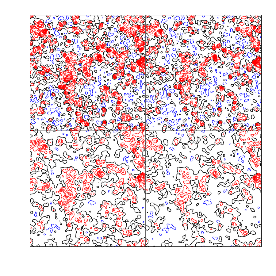
Figure 5: Contour map of the fluctuations in the DBT estimated from the gas density field with $\sigma_{\delta}=1$ at z=15. The panels in the left and right columnn, respectively, correspond to $x_{{}_{\rm HI}}=0.8$ and $0.9$ at $\delta=0$. The top and bottom panels are for frequency bandwidth of $\Delta\nu=10\rm\;KHz$ and $100\rm\;KHz$, respectively. The maps are for an angular resolution of $3.4$ arcmin and the box size is $40\ {\rm h^{-1}Mpc}$ on the side. The solid thick line marks the 8K level of the DBT. Fluctuations below and above the 8K level are represented by the light solid and dotted lines, respectively. The contour spacing is $5\rm\;mK$.

Figure 6: The same as the previous figure but for the gas density field with $\sigma_{\delta}=0.6$. The contour spacing in this map is $3\rm\;mK$.

Figure 7: The $rms$ value of the DBT. The circles are attached to curves obtained from the density field with $\sigma_{\delta}=1$, while the squares are for the fields with $\sigma_{\delta}=0.6$. Solid, dotted, dashed and dash-dotted lines, respectively, correspond to $(\Delta\nu,x_{{}_{\rm HI}})=(100{\rm\;KHz},0.8)$, (10,0.8), (100,0.9), and (10,0.9).

We turn now to the fluctuations along the frequency axis. These are of interest since the correlation along the frequency axis can be extremely useful for disentangling the cosmological signal from foreground contamination (Gnedin & Shaver 2004, Zaldarriaga, Furlanetto & Hernquist 2004). In the top panel of Fig. 8 we plot the DBT fluctuations in a segment of $40\ {\rm h^{-1}Mpc}$ through the numerical box. All curves show DBT in the same segment for a bandwidth of $100\rm\;KHz$, but for different angular resolutions. As is clear from the bottom panel, the DBT is significantly correlated up to separations corresponding to a few $\ {\rm h^{-1}Mpc}$.

Figure 8: Top: The DBT fluctuations in a segment equivalent to $L=40\ {\rm h^{-1}Mpc}$ in the frequency axis. All curves are for the same segment but as seen with different angular resolutions. Bottom: Correlation functions computed from the DBT as a function of frequency. In both panels, all curves for frequency resolution of $\Delta\nu=100\rm\;KHz$, and the solid, dotted, dashed, and dash-dotted lines correspond to angular resolutions of $\Delta\theta=0,0.4,1.6$, and 6.4 arcmin, respectively.

4.3 Brightness temperature in recombination bubbles

In this paper we have focused on 21-cm emission induced by collisions during a pre-reionization period in which X-rays are the main source of ionizing photons. An alternative scenario would be pre-reionization by UV radiation produced by short-lived sources (of lifetime much shorter than the recombination time-scale).

In this scenario re-ionization begins with the production of individual ionized bubbles engulfing the sources. While a bubble recombines electron-atom collisions decouple the spin and CMB temperature efficiently so that significant 21cm emission is possible. The sources also produce Ly$\alpha$ photons which can decouple the CMB from the spin temperature of H I. But, if the filling factor of the bubbles is small and the birth rate of these short lived sources is low then Ly$\alpha$ photons may not become important at the early stages of re-ionization. In a separate paper we will present a detailed analysis of a situation like where the source are identified with massive first stars (e.g. Omukai & Nishi 1998, Abel, Bryan & Norman 2000, Bromm, Coppi & Larson 2002). Here we only consider the differential antenna temperature in a region undergoing recombinations after it has been completely ionized by a short-lived source.

To obtain brightness temperature as a bubble recombines we have numerically integrated the recombination equations assuming Compton cooling (e.g. Peebles 1993) to be the dominant cooler at at the relevant redshifts. The recombination coefficients as a function of temperature are taken from Storey & Hummer (1995). The de-excitation coefficients for atom-atom and atom-electron collisions are from Field (1958), which are in good agreement with other calculations in the literature for $T>100\rm\;K$ (Allison & Dalgarno 1969). In Fig. 9 we plot $\delta T_{\rm b}$ as a function of time for recombinations starting at $z=30$ (solid lines), $z=20$ (dashed lines), and z=15 (dotted). The initial temperature after reionization is taken to be $T_{K}=10^{4}{\rm\;K}$. The three curves in each case correspond to different values of the density contrast inside the bubble: $\delta=1$ (higher curve ), $\delta=0$ (middle curve), and $\delta=-0.3$ (lower curve). We have assumed uniform density inside the bubbles in solving the recombination equations. According to Fig. 9 a recombining bubble can yield a significant 21-cm emission of $\delta T_{\rm b}\sim 10\rm\;mK$ at $\delta~{}\hbox to0.0pt{\raise 1.72218pt\hbox{$>$}\hss}{\lower 3.01385pt\hbox{$\sim$}}~{}0$ for about $10^{8}\rm Yr$ for bubbles generated at $z=15$ and 20. At $z=30$ the emission lasts for a significant fraction of the Hubble time at that redshift. Electron-atom collisions are clearly important even for $\delta=-0.3$. Note that these bubbles can encompass large volumes of space so that the mean density in them is likely to be very close to $\delta=0$. However, density variations inside a bubble will yield $\delta T_{\rm b}$ fluctuations at the level of differences between the curves shown in the figure.

Figure 9: The DBT as a function of time in recombining regions assumed to have been fully ionized at redshift $z=30$ (solid curves), 20 (dashed), and 15 (dotted). The ionizing source is switched off during recombination. The three curves at each redshift, respectively, correspond from top to bottom to mean density contrasts of $\delta=1,$ 0, and $-0.3$ inside the bubbles.

5 Discussion and conclusions

Recently, the cosmological 21-cm signal from the epoch of reionization has been the subject of intensive research activities. Twenty one cm maps are probably the only direct probe of the structure of high redshift reionization. In comparison, secondary CMB anisotropies will provide constraints on line of sight integrated quantities related to the ionized rather than neutral gas. Also, the statistical properties of 21-cm fluctuations contain valuable information on the physical nature of the ionizing sources and the amplitude of the underlying mass at high redshift. Further, it has become clear that the prospects for measuring the 21-cm signal are good in view of the various radio telescopes designed with this purpose in mind. Despite foreground contaminations (e.g. Oh & Mack 2003, Di Matteo, Ciardi & Miniati 2004, Morales & Hewitt 2004, Zaldarriaga, Furlanetto & Hernquist 2004), the collective data obtained by telescopes like the Low Frequency Array (LOFAR), the Primeval Structure Telescope (PAST), the Square Kilometer Array, and the T-Rex instrument should, at the very least, help us discriminate among distinct reionization scenarios.

In some reionization scenarios, collisions of free electrons with H I atoms can lead to a significant 21-cm cosmological signal from regions with density contrasts $(1+\delta)(x_{{}_{\rm HI}}+{\tilde{y}}_{{}_{\rm e}}/{\tilde{y}}_{{}_{\rm HI}}(1-x_{{}_{\rm HI}}))>20[(1+z)/10]^{-2}$ and $x_{{}_{\rm HI}}~{}\hbox to0.0pt{\raise 1.72218pt\hbox{$>$}\hss}{\lower 3.01385pt\hbox{$\sim$}}~{}0.8$, where the ${\tilde{y}}_{{}_{\rm e}}/{\tilde{y}}_{{}_{\rm HI}}$ is in the range $10-20$ (Field 1958). We chose a simplified version of the X-ray pre-reionization scenario as an example for computing the fluctuations in the 21-cm brightness temperature. In this scenario decoupling by collisions is likely to play a major role, at least sufficiently far from the sources. We also demonstrated that collisions are also important during the recombination of gas in bubbles ionized by short lived sources. A recombining bubble should show in 21-cm emission (of $\delta T_{\rm b}\sim 10\rm\;mK$) for about $10^{8}\rm Yr$. A thorough analysis of the collective emission from these bubbles is currently underway.

In order to compute the fluctuations in the X-ray scenario, we have employed a simple semi-analytic model that allows us to assess the statistical properties of 21-cm brightness temperature fluctuations. The 21-cm fluctuations in this and other pre-reionization scenarios have been considered previously by several workers in the field (Bruscoli et al. 2000, Benson et al. 2001, Liu et al. 2001, Iliev et al. 2002, Ciardi & Madau 2003, Bharadwaj & Sk. Saiyad 2004, Ricotti, Ostriker & Gnedin 2004, Zaldarriaga, Furlanetto & Hernquist 2004). In particular Ricotti, Ostriker & Gnedin (2004) used numerical simulations of a $1\ {\rm h^{-1}Mpc}^{3}$ box to model various details of X-ray ionization scenarios. However, an assessment of the importance of collisions vs Ly$\alpha$ pumping as a function of position in the simulation remains to be done. Further, the simulation box is still small and an analysis of the general statistical properties of the fluctuations must rely on semi-analytic models.

We advocate here the the application of the Alcock-Paczyński (AP) test (Alcock & Paczyński 1979) on the correlations measured in three dimensional maps of 21-cm emission. These correlations are readily expressed in terms of angular separations and frequency intervals. In order to derive the correlations in terms of real space separations (measured for example in $\ {\rm h^{-1}Mpc}$) one needs to know the mean density parameter, $\Omega_{\rm m}$, and the cosmological constant $\Omega_{\lambda}$. Constraints on these parameters can then be obtained by demanding isotropy of correlations in real space. A detailed analysis of the 21 cm AP test is presented elsewhere (Nusser 2004).

6 Acknowledgment

The author has benefitted from stimulating discussions with J.P. Ostriker, M.J. Rees, P. Storey, and S. Zaroubi. He wishes to thank the Department of Physics and Astronomy, University College London, for the hospitality and support. This work is supported by the Research and Training Network “The physics of the Intergalactic Medium” set up by the European Community under the contract HPRNCT-2000-00126 and by the German Israeli Foundation for the Development of Research.

References

- [1] Alcock C., Paczyński B., 1979, Nature, 281, 358
- [2] Allison A.C., Dalgarno A., 1969, ApJ, 158, 423
- [3] Baltz E.A, Gnedin N.Y., Silk, J., 1998, ApJ, 493, 1
- [4] Becker et al. 2001, AJ, 122, 2850
- [5] Benson A.J., Nusser A., Sugiyama N., Lacey C., 2001, MNRAS, 320, 153
- [6] Bharadwaj S., Sk. Saiyad, Ali, 2004, MNRAS, 352, 142
- [7] Bi H.G., Boerner G., Chu Y., 1991, A&A, 247, 276
- [8] Bi H.G., 1993, ApJ, 405, 479
- [9] Bi H.G., Davidsen A.F., 1997, ApJ, 479, 523
- [10] Coles P., Jones B., 1991, MNRAS, 248,1
- [11] de Bruyn A.G., 2004, Priv.Comm.
- [12] Bromm V., Coppi P.S., Larson R.B., 2002, ApJ, 564, 23
- [13] Bruscoli M., Ferrara A., Fabbri R., Ciardi B., 2000, MNRAS, 318, 1068
- [14] Cen R., 2003, ApJ, 591, 5
- [15] Chen X., Miralda-Escudé J., 2004, ApJ, 610, 1
- [16] Ciardi B., Madau P., 2003, ApJ, 596, 1
- [17] Croft R.A.C., Weinberg D.H., Hernquist L., Katz N. , 1999, ApJ, 522, 563
- [18] Croft R.A.C., Weinberg D.H., Bolt M., Burles S., Hernquist L., Katz N., Kirkman D., Tytler D., 2002, ApJ, 581, 20
- [19] Dijkstra M., Haiman Z., Loeb A., 2004, ApJ, 613, 646
- [20] Di Matteo T., Ciardi B., Miniati F., 2004, MNRAS, 355, 1035
- [21] Di Matteo T., Perna R., Abel T., Rees M.J., 2002, ApJ, 564, 576
- [22] Field G.B., 1958, Proc, IRE, 46, 240
- [23] Field G.B., 1959, ApJ, 129, 551
- [24] Gnedin Y., Shaver P.A., 2004, ApJ, 608, 611
- [25] Hogan C.J., Rees M.J., 1979, MNRAS, 188, 791
- [26] Hui L., Gnedin N.Y., 1997, ApJ, 486, 599
- [27] Iliev I.T., Scannapieco E., Martel H., Shapiro P.R., 2003, MNRAS, 341, 81
- [28] Iliev I.T, Shapiro P.R., Ferrara A., Martel H., 2002, ApJ, 572, 123
- [29] Kim T.-S., Viel M., Haehnelt M., Carswell R.F., Cristiani S., 2004, MNRAS, 347, 355
- [30] Liu G.C., Sugiyama N., Benson A.J., Nusser A., 2001, MNRAS, 325, 1397
- [31] Madau P., Meiksen A., Rees M.J., 1997, ApJ, 475, 429
- [32] Mather J.C., et al. , 1994, ApJ, 420, 439
- [33] McDonald P., Miralda-Escudé J., Rauch M., Sargent W.L.W., Barlow T.A., Cen R., Ostriker J.P., 2000, ApJ, 543, 1
- [34] McDonald P., Seljak U., Cen R., Weinberg D.H., Burles S., Schneider D.P., Schlegel D.J., Bahcall N.A., Briggs J.W., Brinkmann J., Fukugita M., Ivezic Z., Kent S., Vanden Berk D.E., 2004, astro-ph/0407377
- [35] Machacek M.E., Bryan G.L., Abel T., 2003, MNRAS, 338, 273
- [36] Miniati F., Ferrara A., White S.D.M., Bianchi S., 2004, MNRAS, 348, 964
- [37] Morales M.F., Hewitt J., 2004, ApJ, 615, 7
- [38] Nusser A., Haehnelt M., 1999, MNRAS, 303, 179
- [39] Nusser A., Haehnelt M., 2000, MNRAS, 313, 364
- [40] Nusser A., 2000, MNRAS, 317, 902
- [41] Nusser A., Benson A.J., Sugiyama N., Lacey C., 2002, ApJ, 580, 93
- [42] Nusser A., 2004, astro-ph/0410420
- [43] Oh S.P., Mack K.J., 2003, MNRAS, 346, 871
- [44] Omukai K., Nishi R., 1998, ApJ, 472, 141
- [45] Ostriker J.P., Gnedin N.Y., 1996, ApJ, 472, 63
- [46] Peebles P.J.E., 1980, The Large Scale Structure in the Universe, Princeton Univ. Press.Princeton, NJ
- [47] Peebles P.J.E., 1993, Principles of Physical Cosmology, Princeton Univ. Press.Princeton, NJ
- [48] Peacock J.A., 1999, Cosmological Physics, Cambridge Univ. Press. Cambridge
- [49] Percival W.J., et al. , 2002, MNRAS, 337, 1068
- [50] Ricotti M., Ostriker J., 2004, MNRAS,352, 547
- [51] Ricotti M., Ostriker J., Gnedin N.Y.,2005, MNRAS, 357, 207
- [52] Scott D., Rees M.J., 1990, MNRAS, 247, 510
- [53] Shaver P., Windhorst R., Madau P., de Bruyn G., 1999, A&A, 345, 380
- [54] Spergel D.N. et al. , 2003, ApJS, 148, 175
- [55] Storey P.J., Hummer D.G., 1995, MNRAS, 272, 41
- [56] Sunyaev R.A., Zel’dovich Y.A., 1975, MNRAS, 171,375
- [57] Subramanian K., Padmanabhan T., 1993, MNRAS, 265, 101
- [58] Tozzi P., Madau P., Meiksin A., Rees M.J., 2000, ApJ, 528, 597
- [59] Venkatesan A., Giroux M.L., Shull J.M., 2001, ApJ, 563,1
- [60] Viel M., Matarrese S., Mo H.J., Theuns T., Heahnelt M.G., 2002, MNRAS, 336, 685
- [61] Viel M., Weller J., Haehnelt M., 2004, MNRAS, 355, 23
- [62] Wild J.P., 1952, ApJ, 115, 206
- [63] Wouthuysen S.A., 1952, AJ, 57,31
- [64] Wyithe J.S., Loeb A., 2003, ApJ, 588, 69
- [65] Zaldarriaga M., Furlanetto S.R., Hernquist L., 2004, ApJ, 608, 622
- [66] Zehavi E., et al. , 2002, ApJ, 571, 172