Variability Analysis: Detection and Classification

Abstract

Gaia mission will offer an exceptional opportunity to perform variability studies. The data homogeneity, its optimised photometric systems, composed of 11 medium and 4-5 broad bands, the high photometric precision in G band of one milli-mag for $V=13-15$, the radial velocity measurements and the exquisite astrometric precision for one billion stars will permit a detailed description of variable objects like stars, quasars and asteroids.

However the time sampling and the total number of measurements change from one object to an other because of the satellite scanning law. The data analysis is a challenge because of the huge amount of data, the complexity of the observed objects and the peculiarities of the satellite, and needs a thorough preparation.

Experience can be gained by the study of past and present survey analysis and results and Gaia should be put in perspective with the future large scale surveys, like Pan-STARRS or LSST.

We present the activities of the Variable Star Working Group and a general plan to digest this unprecedented data set, focusing here on the photometry.

1 Introduction

The logarithmic representation of the Universe by Gott et al. (2003)
(http://www.astro.princeton.edu/$\sim$mjuric/universe/) clearly shows the breadth and diversity of the Gaia mission Science.

Gaia will measure targets from the solar system small bodies to the distant quasars, the bulk of objects being 1 billion stars in our Galaxy.

A huge number of the objects will be variable. Indeed asteroids are generally variable at the level $\delta V~{}\sim$ 0.1-0.7 mag. Though the QSOs are sometimes less variable than usually thought (Schechter 2005), a very large fraction of them will be detected as variable with Gaia.

On the side of stars, there is a Zoo of variables: If we look at the GCVS we may count more that 100 types and subtypes. It is customary to divide the variable stars in five main classes: Pulsating stars, eclipsing binaries, variability induced by rotation, eruptive stars and cataclysmic variable stars. The time scale and amplitude of the variation may be very different: from short event of seconds to secular evolution and from milli-magnitudes to several magnitudes. The variability may be periodic, or irregular.

The several instrumental devices on board, photometric, astrometric and radial velocity, will allow a deep investigation on variability induced phenomena. Gaia will allow a global and precise description of stellar variability in terms of physical quantities (temperature, gravity, metallicity). On classical topics, Gaia will give access to absolute masses and sizes for about $10\,000$ eclipsing binaries as pointed out by Zwitter (2003), the period-luminostiy-metallicity realtions of Cepheids will greatly benefit from the parallaxes (cf. Ngeow & Kanbur, these proceedings). Asteroseismology will also benefit from accurate parallaxes, because luminosity and radius are stringent test for the stellar structure, cf. Favata (1999).

The G-band photometric and astrometric informations are deduced from the same CCD counts, therefore an interdependence between the two processings exists. As observed in other surveys, variability may affect astrometric measurements (cf. Pourbaix et al. 2003) and astrometry (proper motions) may affect photometry by the reduction methods, cf. Eyer & Woźniak (2001) or Alcock et al. (2001b). Non uniform light distribution in Long Period Variables (LPVs) may affect the measured astrometry through photocenter wobbling (Jorissen, private communication).

For these reasons, the variability analysis is an unavoidable step of the Gaia mission to improve both scientific returns and astrometric quality.

2 Past Surveys

In recent years, only the hipparcos satellite has done a multi-epoch photometric all-sky survey with an associated analysis aimed at systematically detecting variability. The hipparcos programme consists of 118 204 stars among them a survey of 52 045 stars, complete down to a well defined limiting magnitude function of the star colour and its ecliptic latitude. Results on variable stars were published in the volumes 11 and 12 and among the flags of the main catalogue (ESA 1997). The rate of variable stars is very high, about 10% with a similar rate in the survey and in the preselected star sample.

Microlensing surveys like EROS, MACHO, OGLE detected and characterised a large number of variable stars with a lesser detection rate of about 1%. To mention one, OGLE-II observed about 40 million stars (Udalski et al. (1998), Udalski et al. (2000), Udalski et al. (2002)) and Zebrun et al. (2001) Wozniak et al. (2002) extracted about 290 000 variable stars, data publicly available.

From OGLE and hipparcos surveys, we can see that there is a certain time lag between the data acquisition end and the published results of the variability. The OGLE-II survey collected data from 1997 to 2000, published the photometry for the variable objects in 2001 for the Magellanic clouds and in 2002 for the bulge. In 2004, the database is not fully scientifically exploited yet. Hipparcos finished the measurements in 1993, the catalogue was published in 1997, though the full (prepared) variability analysis was completed within a few months.

These examples show that a thorough preparation of the analysis should be made well in advance in order not to lag with the data flow.

3 Ongoing and Future Surveys

The study of variability for Gaia should also be put in perspective with other projects. A website lists about 90 existing or future robotic telescopes (http://alpha.uni-sw.gwdg.de/$\sim$hessman/MONET/).

We mention here three ongoing surveys:

– ASAS (All-Sky Automated Survey, Pojmanski 1997) is a project which goal is the photometric monitoring of approximately 10 million stars brighter than magnitude 14. The photometry is in $V$ and $I$ bands. The data for variable stars is publicly available. There is an alert system.

– OGLE (Optical Gravitational Lensing Experiment) is continuing to observe the bulge and the Magellanic clouds. It has also dedicated campaigns aiming at the detection of planetary transits (Udalski et al. 2003). OGLE is the first team to have detected planetary systems with the transit method. OGLE-III has a real time analysis Udalski (2003).

– SDSS (Sloan Digital Sky Survey) provides multi-epoch measurements. In the Northern sky, the number of epochs is limited to two but thanks to the multi-colour data, it allows to detect efficiently some variability types cf. Ivezić et al. (2000), Ivezić et al. (2003). We note that in the Southern Survey the number of epochs will be about a dozen.

There are two large scale future surveys which should be mentioned:

– Pan-STARRS (Panoramic Survey Telescope & Rapid Response System) will monitor the sky down to a limiting magnitude of 24 about 20 times per year. The survey will be executed by four 1.8m telescopes located in Hawaii. Each telescope will have a 3 deg field of view. The first light of the first telescope is planned for 2006 and the full system will be operational in 2008. The photometric system will have the Sloan g, r, i bands, a ”sloanish” z band and a y band at 1.7 micron. The photometric precision at the bright end will be about 5 mmag.

– LSST (Large Synoptic Survey Telescope) will cover down to a limiting magnitude of 24 in 5 bands 20 000 square degrees with a single 8.4m telescope. The first light is planned for 2012.

4 Photometric Surveys from Space

Two space missions, COROT and Kepler, will describe as by products the behaviour of large numbers of small amplitude variable stars thanks to their high photometric precision. Two remarkable small satellites, WIRE (Buzasi 2002) and MOST (Walker et al. 2003), have been exploring the small amplitude variability domain working both in a single target mode:

– The CNES/ESA COROT mission (http:// smsc.cnes.fr/COROT/index.htm): The satellite will be in operation from 2006 to 2009 with a possible extension. There will be two programs run in parallel, one dedicated to asteroseismology, the other to planetary transit searches. The exo-planet program will monitor in total 30 000-60 000 stars down to V=15.5 with colour information, in five different fields, during 150 days each. Measurements will be transferred to Earth every 8 minutes. After 1 hour of integration, mean intensities will have a precision of 700 ppm (parts per million) at $V=15.5$. The asteroseismology program will monitor, 5 different fields containing one primary target per field brighter than $V=6$ and a maximum of 9 secondary targets during 150 days. Finally there will be 4 exploratory programs of 30 days each.

– The Kepler Mission (NASA, http:// www.Kepler.NASA.gov/): It will be launched in 2007 and will be operational for 4 years, with a possible 2 year mission extension. At least 100 000 preselected main sequence stars, in the magnitude range from 9 to 15, will be continuously monitored thanks to the Earth-trailing heliocentric orbit and the position of the observed field selected to avoid interruptions in the data acquisition. After 6.5 hours of integration, the mean intensity, for a source of mag V=12, will have a precision of $<$14 ppm (including instrument, background and photon shot noises). Additionally, 200 sources will be monitored for asteroseismological purposes at a one-minute cadence. These source will be changed every 1 to 3 months so as to have monitored all the bright dwarfs in the FOV for p- and g-modes, about 5 000 of them.

5 Gaia Survey

Gaia will observe 1 billion objects with a mean of $\sim$80 measurements in the Astro-field (G-band and Broad Band Photometry-BBP), and $\sim$90 measurements in the Medium Band Photometry (MBP) during 5 years. Possibly a near IR magnitude from the Spectro-field can also be computed. The photometric systems are still under discussions. The photometric precision in the G-band is very high from 1 mmag at V$=$13-15 to 0.02 mag at the limiting magnitude V$=$20; for more details on the photometric performances, see Jordi (2004).

5.1 Gaia Sampling

The satellite will be operated at the second Lagrangian point. The sampling law is governed by two main factors:

1. The rotation of the satellite on itself in 6 hours.

2. The precession of the satellite rotation axis on a cone of 50 deg angle to the Sun, in 70 days.

The Astro-field will gather two observing directions separated by an angle of 106 degrees: the preceding (PFOV) and following (FFOV) fields of view. In the Astro-field, a star has measurements generally grouped consecutively with the time intervals of 1h46, 4h14, 1h46, etc, corresponding to observations in the PFOV-FFOV-PFOV, etc. Then the next group will occur typically 30 days later. Both the total length of the sequence of short consecutive measurements and the time intreval between the grouped measurements depend on the position of the star on the celestial sphere. We show in Figure 1 the dependence on the number of measurements as function of the ecliptic latitude $\beta$. The mean number of measurements is 82 but varies between 45 to 210.

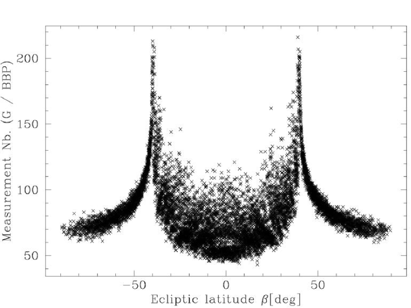
Figure 1: Number of measurements (transits) as function of the ecliptic latitude $\beta$. The mean number of measurements is 82.

5.2 Number of variable objects detected by Gaia

The number of variable objects detected by Gaia is still quite uncertain. First estimations done by Eyer & Cuypers (2000) lead to about 18 million classical variable stars.

Caution is still needed: for instance the estimates of the number of eclipsing binaries by different authors differ greatly: Soederhjelm (private communication) estimated this number to be half a million, whereas Eyer & Cuypers (2000) estimated it to 2-3 millions and Zwitter (2002) to 7 millions.We list several estimates for other variable types:

– Eyer & Cuypers (2000) estimated the numbers of RR Lyr to 70 000, of Cepheids to 2 000-8 000, of Mira-LPVs to 200 000, of $\delta\,$Scuti stars to 60 000-240 000, of SPBs to 15 000, of $\beta\,$ Cep stars to 3 000.
– Robichon (2002, private communication) estimated the number of planetary transit systems to 5 000-30 000.
– Belokurov & Evans (2003) estimated the number of Supernovae to 21 000.
– Totani & Panaitescu (2002) estimated that Gaia will observe 720 optical counter parts of gamma ray bursts.

5.3 Rate of correct detection of Periods

Eyer and Mignard has investigated the rate of correct detection of the period for a given periodic signal observed with the Gaia sampling law. Sinusoidal signals have been generated for pairs of $P$ (period) and $Q$ (amplitude to noise ratio) and sampled with the Gaia scanning law for 10 000 stars uniformly distributed over the celestial sphere. For each star a periodogram is constructed, and the highest power period $P_{h}$ is confronted to the true period $P$. About 1.4 million periodograms have been computed.

As expected, the rate of correct period detection depends on the number of measurements and therefore on the ecliptic latitude. Once the number of measurements effect is corrected, the dependence on the ecliptic latitude does not fully vanish. A dip reaching 10–15% in the period correct detection rate is still present at ecliptic latitude 20 degrees.

Very high amplitude to noise ratio $Q$ is not necessary to recover the period. Already at $Q=1.3$, the rate of correct detection is mostly above 90%. For example a sinusoidal signal of amplitude 3 mmag at $V=14$, will have its period correctly recovered from several hours to hundreds of days.

5.4 Variable Star Working Group activities

In the previous sections we covered some activities of the Working Group. They are fully described at the following website:

http://obswww.unige.ch/~eyer/VSWG/

You may find more information on:
– Variable star characteristics: We prepare a uniform description of variable star types. Information collected are: general references, physical properties, variability properties (times scales and amplitudes of the photometric and radial velocity variations), physical source of variability, number of star known, fraction of variable is the same area of the HR diagram. Once the filters of Gaia will be defined, variability at the filter wavelengths will be estimated for each type. Such characteristics will serve for completing the Galactic Model used for GDAAS (Gaia Data Access and Analysis Study), for the estimation of the number of variables, as well as for the classification.

– Compilations of past, present and future surveys: We want to keep track of the research done on these surveys. Therefore we give a list of past surveys with their returns on variable stars. We will add the methods used to analyse the data. We will also give the characteristics of some future surveys.

– Forecasts about variable stars to be detected by Gaia: We gather published information from different researchers on the forecasts.

– Tools: We give a list of typical tools which are used in variable star research. Algorithms of Period search, time scales, or classification methods. We put online software for some algorithms, or links to the codes whenever possible.

– GDAAS related activities: We are developing software for the GDAAS analysis (see the following section).

6 Global analysis

The variability analysis can be seen as a process of data compression. If a star has a constant magnitude, then the whole time series can be summarised by two quantities (per band): the mean magnitude and its precision. For instance the compression factor for the G-band photometry with 80 measurements is about 140 (the measurement epochs can be removed). If the object is detected as variable, then the task to compress the data is more laborious, the time series may be reduced, for example, to amplitude(s), time-scale(s), period(s), epochs, parameters of Fourier series, variable types. The goals of the global analysis are to separate the observed objects in constant (or more precisely non detected as variable) and variable, and to reach a classification with the associated relevant parameters. We proposed an organigram to fulfil these goals in Figure 2.

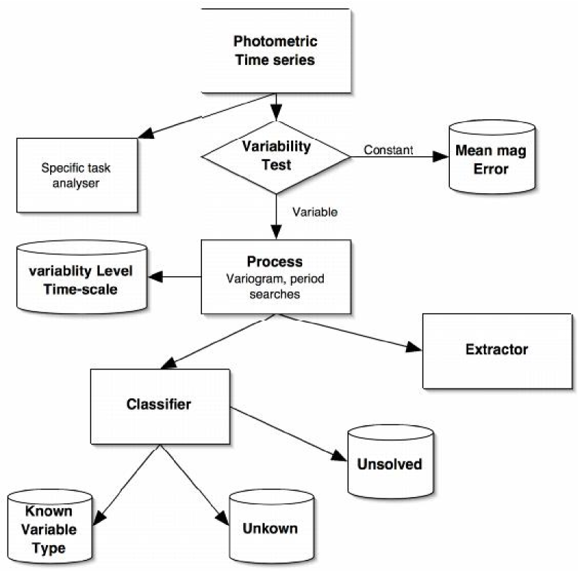
Figure 2: Organigram of used data processing of the variable stars, baseline of the current development of the software for GDAAS.

6.1 Detection of variability

The first step is to detect variability. As different variability behaviours have different photometric signatures, a set of different statistical tests had to be designed.

Thanks to the very high G-magnitude precision, it has been decided, during the VSWG Cambridge meeting in 2004, to use the magnitudes deduced from one passage of the observed object over the 11 CCDs of the Astro-field. Studies of very short term variability should also be explored using the per CCD information (most algorithms developed for the per transit analysis are applicable at this level).

To detect variability we perform a number of statistical tests on the G-band photometric data. For these tests two aspects are important:

1. they should be mathematically formulated in a cumulative way, so that during the mission, when new data are coming, the values of the statistical tests can be updated from old cumulated quantities and the new data. So, the variability status of every object can be monitored.

2. for each test and observed time series, p-values will be computed. In the framework of hypothesis testing under the null hypothesis, a p-value is the probably of observing a value more extreme than the one actually observed. It allows to set a variability detection threshold independent of the number of measurements and of the noise level.

The chosen tests are the $\chi^{2}$ test, tests on the asymmetry and kurtosis (these tests are related to three moments of the distribution), Abbe test (von Newmann 1941), a test to detect outliers, and a test on the presence of a slope.

The stellar variability for certain variable types may remain undetected in a wide band filter like the G-band because of compensation effects in the spectral interval covered by the G-band. The MBP and BBP bands will also be used. One method is to compute the covariant matrix between the different bands $M_{k,l}=\sum_{i=1}^{n}(m_{k,i}-\overline{m_{k}})(m_{l,i}-\overline{m_{l}})/(\sigma_{k,i}\sigma_{l,i})$, where $n$ is the number of measurements, the indices $k,l$ refer to the available photometric bands and $\overline{m_{l}}$ the mean $l$-magnitude. The matrix diagonal terms are the values associated to the $\chi^{2}$. If we diagonalise the matrix then we will get a signature of the physical nature of the variability. It seems an elegant way to combine the information of different filters and to enhance the variability detection capability. We will perform some tests on the five Sloan filters of SDSS data and also on simulated data generated from synthetic spectra.

6.2 Modelling the variability

Once the variability is detected. Some further processing is require to characterise the variability.

For strictly periodic behaviours, periodograms can be computed and the period of highest ”power” can be used. There is no method which is superior to all the others for finding the period of a periodic signal, some are performing better for certain types of behaviour, some others are more less prone to certain types of aliasing. The CPU consumption time may be also very different, though some optimisation are possible. We plan, as activities of the working group, to start benchmarking of these different methods. Simple method to recognise mono-periodic and multi-periodic phenomena should be also planed.

Fourier series are adequate mathematical representation to model periodic variability (though often problematic for EA eclipsing binaries). However it appears difficult to separate a set of well behaved light curves even after a Fourier decomposition with analysis of residues (Eyer & Blake 2004).

If the star is irregular, we have to rely on more general description:

– The amplitude of variation: Several estimations are found in the literature. It is customary to give magnitudes at minimum and maximum light, however these quantities are not robust to outliers, and are meaningless if the amplitude of variation is small compared to the noise measurements. There are other estimations: signal variance, inter-quartile (-decile) range, estimated amplitudes correct from noise measurements.

– Time scales: The power spectrum can be used as a general description of the signal behaviour Evans & Belokurov (2004). Calculation of variogram or auto-correlation algorithms maybe useful tools to provide time scales, when both the variable object and the time sampling are irregular

These questions will be addressed.

6.3 Classification

We distinguish between two different strategies: a global approach to classification and an extraction of certain variable types.

Mostly what has been done in the microlensing surveys is to extract some specific variability types. Criteria have been designed for known variable types, some few examples: RR Lyrae stars Alcock et al. (2000), R Coronae Borealis Stars Alcock et al. (2001a), etc, from MACHO data, Cepheids (Udalski et al. 1999), eclipsing binaries (Wyrzykowski et al. 2004), etc, from OGLE data. On Hipparcos data, multivariate discriminant analysis has been applied to extract Slowly Pulsating B stars, and $\gamma\,$Dor stars, cf. Waelkens et al. (1998), Aerts et al. (1998).

For the moment very few attempts of global classification have been done, examples can be found in Pojmanski & Maciejewski (2004) on ASAS data, Eyer & Blake (2004) on ASAS data, Belokurov et al. (2003) on MACHO data, Wozniak et al. (2001), on ROTSE data, Marquette (private communication) on EROS data.

We are therefore nowadays in a stage of method exploration. Very promising methods like Self-Organising Maps (SOMs) are studied, see Evans & Belokurov (2004) for a description of the method, cf. also Brett et al. (2004). Dr A. Naud (Torun Unversity) started a study on the global classification with SOMs of the Hipparcos periodic variable star catalogue. This classification is using for each variable star its period, amplitude, colour V-I and the skewness of the photometric time series. The result is displayed in Figure 3. We observe that the classes of Mira, SRs, Cepheids and eclipsing binaries form isolated groups. The smaller amplitude variables are somewhat mixed.

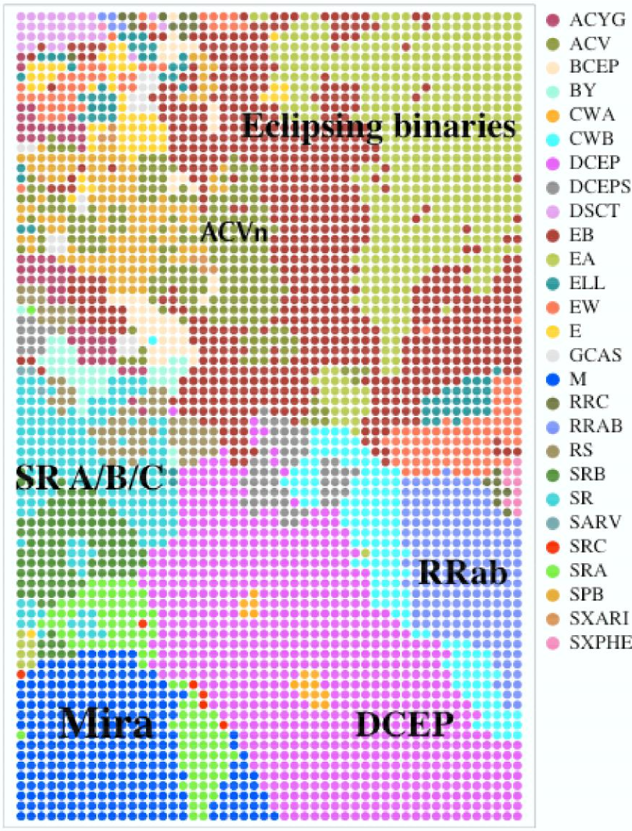
Figure 3: Classification of hipparcos periodic variable star catalogue with Self-Organising Maps by Dr A. Naud.

Several classification methods should be studied and compared: their efficiency, their capability to separate classes, their ability to detect new classes, their error levels, their robustness with respect to the sampling, their CPU consumption, and their level of required human interaction.

Once some objects are recognised, further analysis can be done. Global treatment of eclipsing binaries have been done on OGLE data by Wyithe & Wilson (2001), Wyithe & Wilson (2002) and are investigated for the Gaia mission by Prša & Zwitter (2004).

Many tests can be run on existing surveys like ASAS, MACHO, EROS, OGLE. However we remind that the wealth of Gaia data is larger, the precision is higher and as for Hipparcos, the sampling is peculiar. Global classification studies will have to be done with GDAAS.

The global classification is not excluding procedures of specific tasks, selecting unusual and rare objects. As an example of an special selection procedure, we mention the detected hipparcos planetary transits of HD 209458, cf. Robichon & Arenou (2000) and Soderhjelm (1999). It could have been singled out in Hipparcos before the discovery of Charbonneau et al. (2000). The HD 209458 hipparcos photometric time series was not classified as variable, the eclipse depth is very shallow with respect to the measurement noise, however with a well tailored statistical test ran on a subsample of Hipparcos sources, HD 209458 is one of the best candidate for having possible transits.

7 Conclusion

We have started to write algorithms for GDAAS to analyse the photometric time series. If the Gaia launch date of 2011 seems far away, the tasks required to analyse the Gaia data for variability studies are enormous. If a general picture of the variability analysis is present, many problems are not solved yet. In order to gauge correctly the efficiency of proposed methods, of the analysis as a whole, there is the need to study thoroughly very technical details.

There are also broader questions: how and when to deliver intermediate results on variable objects during the mission, how to plan Earth follow-up observations, how to combine Gaia data with coeval surveys, what tools to use for the visualisation of Gaia data and the quantities results of the variability analysis.

If Gaia data will be an unprecedented data set, the variability analysis also requires unprecedented ingenious methods, software developments and collaborative efforts of many researchers.

References

- Aerts et al. (1998) Aerts, C., Eyer, L., & Kestens, E. 1998, A&A, 337, 790
- Alcock et al. (2000) Alcock, C., Allsman, R., Alves, D. R., et al. 2000, ApJ, 542, 257
- Alcock et al. (2001a) Alcock, C., Allsman, R. A., Alves, D. R., et al. 2001a, ApJ, 554, 298
- Alcock et al. (2001b) —. 2001b, ApJ, 562, 337
- Belokurov et al. (2003) Belokurov, V., Evans, N. W., & Du, Y. L. 2003, MNRAS, 341, 1373
- Belokurov & Evans (2003) Belokurov, V. A. & Evans, N. W. 2003, MNRAS, 341, 569
- Brett et al. (2004) Brett, D. R., West, R. G., & Wheatley, P. J. 2004, MNRAS, 353, 369
- Buzasi (2002) Buzasi, D. 2002, in ASP Conf. Ser. 259: IAU Colloq. 185: Radial and Nonradial Pulsationsn as Probes of Stellar Physics, 616–+
- Charbonneau et al. (2000) Charbonneau, D., Brown, T. M., Latham, D. W., & Mayor, M. 2000, ApJ, 529, L45
- ESA (1997) ESA. 1997, ESA SP-1200
- Evans & Belokurov (2004) Evans, N. W. & Belokurov, V. A. 2004, in this volume
- Eyer & Blake (2004) Eyer, L. & Blake, C. 2004, astro-ph/0406333
- Eyer & Cuypers (2000) Eyer, L. & Cuypers, J. 2000, in ASP Conf. Ser. 203: IAU Colloq. 176: The Impact of Large-Scale Surveys on Pulsating Star Research, 71–72
- Eyer & Woźniak (2001) Eyer, L. & Woźniak, P. R. 2001, MNRAS, 327, 601
- Favata (1999) Favata, F. 1999, Baltic Astronomy, 8, 309
- Gott et al. (2003) Gott, J. R., Jurić, M., Schlegel, D., et al. 2003, astro-ph/0310571
- Ivezić et al. (2000) Ivezić, Ž., Goldston, J., Finlator, K., et al. 2000, AJ, 120, 963
- Ivezić et al. (2003) Ivezić, Ž., Lupton, R. H., Anderson, S., et al. 2003, Memorie della Societa Astronomica Italiana, 74, 978
- Jordi (2004) Jordi, C. 2004, in this volume
- Pojmanski (1997) Pojmanski, G. 1997, Acta Astronomica, 47, 467
- Pojmanski & Maciejewski (2004) Pojmanski, G. & Maciejewski, G. 2004, Acta Astronomica, 54, 153
- Pourbaix et al. (2003) Pourbaix, D., Platais, I., Detournay, S., et al. 2003, A&A, 399, 1167
- Prša & Zwitter (2004) Prša, A. & Zwitter, T. 2004, in this volume
- Robichon & Arenou (2000) Robichon, N. & Arenou, F. 2000, A&A, 355, 295
- Schechter (2005) Schechter, P. 2005, ASP Conf. Ser. x: IAU Symp. 225
- Soderhjelm (1999) Soderhjelm, S. 1999, Informational Bulletin on Variable Stars, 4816, 1