The multi-frequency angular power spectrum of the epoch of reionization 21 cm signal

Abstract

Observations of redshifted 21cm radiation from neutral hydrogen (HI) at high redshifts is an important future probe of reionization. We consider the Multi-frequency Angular Power Spectrum (MAPS) to quantify the statistics of the HI signal as a joint function of the angular multipole $l$ and frequency separation $\Delta\nu$. The signal at two different frequencies is expected to decorrelate as $\Delta\nu$ is increased, and quantifying this is particularly important in deciding the frequency resolution for future HI observations. This is also expected to play a very crucial role in extracting the signal from foregrounds as the signal is expected to decorrelate much faster than the foregrounds (which are largely continuum sources) with increasing $\Delta\nu$.

In this paper we develop formulae relating MAPS to different components of the three dimensional HI power spectrum taking into account HI peculiar velocities. We show that the flat-sky approximation provides a very good representation over the angular scales of interest, and a final expression which is very simple to calculate and interpret. We present results for $z=10$ assuming a neutral hydrogen fraction of $0.6$ considering two models for the HI distribution, namely, (i) DM: where the HI traces the dark matter and (ii) PR: where the effects of patchy reionization are incorporated through two parameters which are the bubble size and the clustering of the bubble centers relative to the dark matter (bias) respectively. We find that while the DM signal is largely featureless, the PR signal peaks at the angular scales of the individual bubbles where it is Poisson fluctuation dominated, and the signal is considerably enhanced for large bubble size. For most cases of interest at $l\sim 100$ the signal is uncorrelated beyond $\Delta\nu\sim 1\,{\rm MHz}$ or even less, whereas this occurs around $\sim 0.1\,{\rm MHz}$ at $l\sim 10^{3}$. The $\Delta\nu$ dependence also carries an imprint of the bubble size and the bias, and is expected to be an important probe of the reionization scenario. Finally we find that the $l$ range $10^{3}-10^{4}$ is optimum for separating out the cosmological HI signal from the foregrounds, while this will be extremely demanding at $l<100$ where it is necessary to characterize the $\Delta\nu$ dependence of the foreground MAPS to an accuracy better than $1\%$.

1 Introduction

One of the major challenges in modern cosmology is to understand the reionization history of the Universe. Numerous attempts have been made in this regard to constrain the evolution of neutral hydrogen density (for recent reviews, see Barkana & Loeb 2001; Fan, Carilli & Keating 2006; Choudhury & Ferrara 2006a). Analyzes of quasar absorption spectra suggest that almost all of the hydrogen has been ionized around redshift $z<6$ (Becker et al. 2001; Fan et al. 2002). A different set of constraints come from the Cosmic Microwave Background (CMB) observations. The CMB photons scatter with free electrons (produced because of reionization) which result in the suppression of the intrinsic anisotropies; at the same time a polarization signal is generated from this scattering. Measurements of the electron scattering optical depth from recent CMB observations like WMAP (Spergel et al. 2006; Page et al. 2006) imply that reionization started before $z\sim 10$. It thus seems from these two results that reionization is an extended and complex process occurring over a redshift range 6–15 (Choudhury & Ferrara 2006b; Alvarez et al. 2006). However, there exist limitations of using these observations to study the details of reionization process which would be occurring at redshifts $\approx 10$. At present there is no indication of quasars at such high redshifts; on the other hand, the electron scattering optical depth is sensitive only to the integral history of reionization and it may not be useful to study the progress of reionization with redshift. In fact, it has been shown that the CMB polarization power spectrum is weakly dependent on the details of the reionization history (Kaplinghat et al. 2003; Hu & Holder 2003; Haiman & Holder 2003; Colombo 2004), though weak constraints could be obtained from upcoming experiments such as PLANCK.

Perhaps the most promising prospect of studying reionization at various stages of its progress is through future 21 cm observations(for recent review see Furlanetto et al. (2006)). This basically involves observing the redshifted 21 cm line from the neutral hydrogen (HI) at high redshifts. The advantage of these experiments lie in the fact that one can track neutral hydrogen fraction at any desired redshift by appropriately tuning the observation frequency. Tomography of the HI distribution using observations of the redshifted 21 cm line is one of the most promising tool to study reionization.

The possibility of observing 21 cm emission from the cosmological structure formation was first recognized by Sunyaev and Zeldovich (1972) and later studied by Hogan & Rees (1979), Scott & Rees (1990) and Madau, Meiksin & Rees ((1997)) considering both emission and absorption against the CMB. More recently, the effect of heating of the HI gas and its reionization on 21 cm signal has drawn great deal of attention and has been studied in detail (Gnedin & Ostriker 1997; Shaver et al. 1999; Tozzi et al. 2000; Iliev et al. 2002, 2003; Ciardi & Madau 2003; Furlanetto, Sokasian & Hernquist 2004; Miralda-Escude 2003; Chen & Miralda-Escude 2004; Cooray & Furlanetto 2005; Cooray 2005; Mcquinn et al. 2005; Sethi 2005; Salvaterra et al. 2005; Carilli 2006).

It is currently perceived that a statistical analysis of the fluctuations in the redshifted 21 cm signal which is present as a minute component of the background radiation in all low frequency radio observations holds the greatest potential. This approach has been considered in the context of lower redshifts (Bharadwaj, Nath & Sethi 2001; Bharadwaj & Sethi 2001; Bharadwaj & Pandey 2003; Bharadwaj & Srikant 2004). A similar formalism can also be applied at high redshifts to probe reionization and also the pre-reionization era (Zaldarriaga, Furlanetto & Hernquist 2004; Furlanetto, Zaldarriaga & Hernquist 2004b; Morales & Hewitt 2004; Bharadwaj & Ali 2004, 2005; Bharadwaj & Pandey 2005; Ali, Bharadwaj and Pandey 2005; Ali, Bharadwaj and Pandey 2006; Loeb & Zaldarriaga 2004; He et al. 2004). One of the main aims of epoch of reionization 21 cm studies is to probe the size, spatial distribution and evolution of the ionized regions which has been addressed by several groups (Furlanetto, McQuinn & Hernquist 2006; Furlanetto, Zaldarriaga & Hernquist 2004a; Wyithe & Loeb 2004; Mellema et al. 2006; Iliev et al. 2005).

On the observational front, several initiatives are currently underway. The Giant Metre-Wave Radio Telescope (GMRT; Swarup et al. 1991) is already functioning at several bands in frequency range 150-1420 MHz and can potentially detect the 21 cm signal at high redshifts. In addition, upcoming low-frequency experiments such as LOw Frequency ARray (LOFAR), Square Kilometer Array (SKA), PrimevAl Structure Telescope (PAST) have now raised the possibility to detect 21 cm signal from very high redshift and thus motivated a detailed study of the expected 21 cm background from neutral hydrogen at high redshifts.

Although the redshifted 21 cm line can provide enormous amounts of information, its detection is going to be a huge challenge. The signal is expected to be highly contaminated by foreground radio emission. Potential sources for these foregrounds include synchrotron and free-free emission from or Galaxy and external galaxies, low-frequency radio point sources and free emission from electrons in the intergalactic medium (Shaver et al. 1999; DiMatteo. et al. 2002, 2004; Oh 1999; Cooray & Furlanetto 2004). Since these foregrounds are much stronger than the 21 cm signal arising from HI, it has been suggested that it may be impossible to study reionization via such observations (Oh & Mack 2003).

However, there have been various proposals for tackling such foregrounds, the most promising being the usage of multi-frequency observations. It has been proposed that multi-frequency analysis of the radio signal can be useful in separating out the foreground (see e.g. Shaver et al. 1999; DiMatteo. et al. 2002; Gnedin & Shaver 2004; DiMatteo. et al. 2004; Santos, Cooray & Knox 2005). In fact this has also been noted by most of the authors who have studied the statistical signal from redshifted HI and have been referred to earlier. The cross correlation between the HI signal at different frequencies is expected to decay rapidly as the frequency separation is increased (Bharadwaj & Ali 2005; Santos, Cooray & Knox 2005) while the foregrounds are expected to have a continuum spectrum and hence should be correlated across frequencies. This property of different foregrounds contaminants can in principle be used to remove them from expected 21 signal.

In this paper, we develop the formalism to calculate the multi-frequency angular power spectrum (hereafter MAPS) which can be used to Analise the 21 cm signal from HI both in emission and absorption against the CMB. We restrict our attention to HI emission which is the situation of interest for the epoch of reionization. In our formalism, we consider the effect of redshift-space distortions which has been ignored in many of earlier works. As noted by Bharadwaj & Ali (2004), this is an important effect and can enhance the mean signal by $50\%$ or more and the effect is expected to be most pronounced in the multi-frequency analysis. We next use the flat sky approximation to develop a much simpler expression of MAPS which is much easier to calculate and interpret than the angular power spectrum written in terms of the spherical Bessel functions. We adopt a simple model for the HI distribution (Bharadwaj & Ali, 2005) which incorporates patchy reionization and use it to predict the expected signal and study its multi-frequency properties. The model allows us to vary properties like the size of the ionized regions and their bias relative to the dark matter. We use MAPS to analyze the imprint of these features on the HI signal and discuss their implication for future HI observations.

As noted earlier, the HI signal at two different frequencies separated by $\Delta\nu$ is expected to become uncorrelated as $\Delta\nu$ is increases. As noted in Bharadwaj & Ali (2005), the value of $\Delta\nu$ beyond which the signal ceases to be correlated depends on the angular scales being observed and it is $<1\,{\rm MHz}$ in most situations of interest. A prior estimate of the multi-frequency behavior is extremely important when planning HI observations. The width of the individual frequency channels sets the frequency resolution over which the signal is averaged. This should be chosen sufficiently small so that the signal remains correlated over the channel width. Choosing a frequency channel which is too wide would end up averaging uncorrelated HI signal which would wash out various important features in the signal, and also lead to a degradation in the signal to noise ratio. In this context we also note that an earlier work (Santos, Cooray & Knox, 2005) assumed individual frequency channels $1\,{\rm MHz}$ wide and smoothed the signal with this before performing the multi-frequency analysis. This, as we have already noted and shall study in detail in this paper, is considerably larger than the $\Delta\nu$ where the signal is uncorrelated and hence is not the optimal strategy for the analysis. We avoid such a pitfall by not incorporating the finite frequency resolution of any realistic HI observations. It is assumed that the analysis of this paper be used to determine the optimal frequency channel width for future HI observations. Further, it is quite straightforward to introduce a finite frequency window into our result through a convolution.

The outline of this paper is as follows. In Section 2 we present the theoretical formalism for calculating MAPS of the expected 21 cm signal considering the effect of HI peculiar velocity. The calculation in the full-sky and the flat-sky approximation are both presented with the details being given in separate Appendices. Section 2.1 defines various components of the HI power spectrum and Section 2.4 presents to models for the HI distribution. We use these models when making predictions for the expected HI signal. We present our results in Section 3 and also summarize our findings. In Section 4. we discuss the implications for extracting the signal from the foregrounds.

2 Theoretical Formalism

2.1 The HI power spectrum

The aim of this section is to set up the notation and calculate the angular correlation $C_{l}$ for the 21cm brightness temperature fluctuations. It is now well known (e.g.. Bharadwaj & Ali 2005) that the excess brightness temperature observed at a frequency $\nu$ along a direction ${\bf\hat{n}}$ is given by

$$T(\nu,{\bf\hat{n}})=\bar{T}(z)~{}\eta_{\rm HI}\left(z,{\bf\hat{n}}r_{\nu}\right)$$ (1)

where the frequency of observation is related to the redshift by $\nu=1420/(1+z)\,{\rm MHz}$. The quantity

$$r_{\nu}=\int_{0}^{z}{\rm d}z^{\prime}\frac{c}{H(z^{\prime})}$$ (2)

is the comoving distance and

$$\bar{T}(z)\approx 25{\rm mK}\sqrt{\frac{0.15}{\Omega_{m}h^{2}}}~{}\left(\frac{\Omega_{B}h^{2}}{0.022}\right)\left(\frac{1-Y}{0.76}\right)\sqrt{\frac{1+z}{10}}$$ (3)

where $Y\approx 0.24$ is the helium mass fraction and all other symbols have usual meaning. In the above relation, it has been assumed that the Hubble parameter $H(z)\approx H_{0}\Omega_{m}^{1/2}(1+z)^{3/2}$, which is a good approximation for most cosmological models at $z>3$. The quantity $\eta_{\rm HI}$ is known as the “21 cm radiation efficiency in redshift space” (Bharadwaj & Ali 2005) and can be written in terms of the mean neutral hydrogen fraction $\bar{x}_{\rm HI}$ and the fluctuation in neutral hydrogen density field $\delta_{\rm HI}$ as

$$\eta_{\rm HI}(z,{\bf\hat{n}}r_{\nu}) = \bar{x}_{\rm HI}(z)[1+\delta_{\rm HI}(z,{\bf\hat{n}}r_{\nu})]\left(1-\frac{T_{\gamma}}{T_{s}}\right)$$ (4)

$$\times \left[1-\frac{(1+z)}{H(z)}\frac{\partial v(z,{\bf\hat{n}}r_{\nu})}{\partial r_{\nu}}\right]$$

where $T_{\gamma}$ and $T_{s}$ are the temperature of the CMB and the spin temperature of the gas respectively. The term in the square bracket arises from the coherent components of the HI peculiar velocities.

At this stage, it is useful to make a set of assumptions which will simplify our analysis: (i) We assume that $T_{s}\gg T_{\gamma}$, which corresponds to the scenario where the intergalactic gas is heated well above the CMB temperature during the reionization process. This assumption is expected to be valid throughout the IGM soon after the formation of first sources of radiation as a substantial background of X-rays from supernovae, star-formation, etc. can heat the IGM quickly. (ii) We assume that the HI peculiar velocity field is determined by the dark matter fluctuations, which is reasonable as the peculiar velocities mostly trace the dark matter potential wells. We then have

$$\eta_{\rm HI}(z,{\bf\hat{n}}r_{\nu})=\int\frac{{\rm d}^{3}k}{(2\pi)^{3}}{\rm e}^{-{\rm i}kr_{\nu}({\bf\hat{k}\cdot\hat{n}})}\tilde{\eta}_{\rm HI}\left(z,{\bf k}\right)$$ (5)

where

$$\tilde{\eta}_{\rm HI}\left(z,{\bf k}\right)=\bar{x}_{\rm HI}(z)\left[\Delta_{\rm HI}(z,{\bf k})+({\bf\hat{k}\cdot\hat{n}})^{2}\Delta(z,{\bf k})\right]\,,$$ (6)

and $\Delta_{\rm HI}(z,{\bf k})$ and $\Delta(z,{\bf k})$ are the Fourier transform of the fluctuations in the HI and the dark matter densities respectively. Note that $f(\Omega_{m})$, which relates peculiar velocities to the dark matter, has been assumed to have a value $f(\Omega_{m})=1$ which is reasonable at the high $z$ of interest here.

For future use, we define the relevant three dimensional (3D) power spectra

$$\langle\Delta(z,{\bf k})\Delta^{*}(z,{\bf k^{\prime}})\rangle = (2\pi)^{3}\delta_{D}({\bf k-k^{\prime}})P(z,k)$$

$$\langle\Delta_{\rm HI}(z,{\bf k})\Delta^{*}_{\rm HI}(z,{\bf k^{\prime}})\rangle = (2\pi)^{3}\delta_{D}({\bf k-k^{\prime}})P_{\Delta^{2}_{\rm HI}}(z,k)$$

$$\langle\Delta(z,{\bf k})\Delta^{*}_{\rm HI}(z,{\bf k^{\prime}})\rangle = (2\pi)^{3}\delta_{D}({\bf k-k^{\prime}})P_{\Delta_{\rm HI}}(z,k)$$ (7)

where $P(z,k)$ and $P_{\Delta^{2}_{\rm HI}}(z,k)$ are the power spectra of the fluctuations in the dark matter and the HI densities respectively, while $P_{\Delta_{\rm HI}}(z,k)$ is the cross-correlation between the two.

2.2 The multi-frequency angular power spectrum (MAPS)

The multi-frequency angular power spectrum of 21 cm brightness temperature fluctuations at two different frequencies $\nu_{1}$ and $\nu_{2}$ is defined as

$$C_{l}(\nu_{1},\nu_{2})\equiv\langle a_{lm}(\nu_{1})~{}a^{*}_{lm}(\nu_{2})\rangle\,.$$ (8)

In our entire analysis $\nu_{1}$ and $\nu_{2}$ are assumed to differ by only a small amount $\Delta\nu\ll\nu_{1}$, and it is convenient to introduce the notation

$$C_{l}(\Delta\nu)\equiv C_{l}(\nu,\nu+\Delta\nu)$$ (9)

where we do not explicitly show the frequency $\nu$ whose value will be clear from the context. Further, wherever possible, we shall not explicitly show the $z$ dependence of various quantities like $\bar{T}$, $\bar{x}_{\rm HI}$, $P(k)$ etc., and it is to be understood that these are to be evaluated at the appropriate redshift determined by $\nu$.

The spherical harmonic moment of $T(\nu,{\bf\hat{n}})$ are defined as

$$a_{lm}(\nu) = \int{\rm d}\Omega~{}Y^{*}_{lm}({\bf\hat{n}})~{}T(\nu,{\bf\hat{n}})$$

$$= \bar{T}\int{\rm d}\Omega~{}Y^{*}_{lm}({\bf\hat{n}})~{}\int\frac{{\rm d}^{3}k}{(2\pi)^{3}}\tilde{\eta}_{\rm HI}\left({\bf k}\right){\rm e}^{-{\rm i}kr_{\nu}({\bf\hat{k}\cdot\hat{n}})}\,.$$

Putting the expression (6) for $\tilde{\eta}_{\rm HI}\left({\bf k}\right)$ in the above equation, one can explicitly calculate the MAPS in terms of the three dimensional power spectra defined earlier. We give the details of the calculation in Appendix A and present only the final expression for the angular power spectrum at a frequency $\nu$

$$C_{l}(\Delta\nu)\!\!\!\!\! = \!\!\!\!\!\frac{2\bar{T}^{2}~{}\bar{x}^{2}_{\rm HI}}{\pi}\int_{0}^{\infty}k^{2}{\rm d}k\,\left[j_{l}(kr_{\nu})j_{l}(kr_{\nu_{2}})P_{\Delta^{2}_{\rm HI}}(k)\right.$$

$$- \!\!\!\!\!\{j_{l}(kr_{\nu})j^{\prime\prime}_{l}(kr_{\nu_{2}})+j_{l}(kr_{\nu_{2}})j^{\prime\prime}_{l}(kr_{\nu})\}P_{\Delta_{\rm HI}}(k)$$

$$+ \!\!\!\!\!\left.j^{\prime\prime}_{l}(kr_{\nu})j^{\prime\prime}_{l}(kr_{\nu_{2}})P(k)\right]$$

Here $j^{\prime\prime}_{l}(x)=\frac{d^{2}}{dx^{2}}j_{l}(x)$ and we have used the notation $r_{\nu_{2}}=r_{\nu}+r^{\prime}_{\nu}~{}\Delta\nu$ with

$$r^{\prime}_{\nu}\equiv\frac{\partial r_{\nu}}{\partial\nu}=-\frac{c}{\nu_{0}}\frac{(1+z)^{2}}{H(z)}.$$ (12)

Note that equation (2.2) predicts $C_{l}(\Delta\nu)$ from the cosmological 21 cm HI signal to be real.

With increasing $\Delta\nu$, we expect the two spherical Bessel functions $j_{l}(kr_{\nu_{1}})$ and $j_{l}(kr_{\nu_{2}})$ to oscillate out of phase. As a consequence the value of $C_{l}(\Delta\nu)$ is expected to fall increasing $\Delta\nu$. We quantify this through a dimensionless frequency decorrelation function defined as the ratio

$$\kappa_{l}(\Delta\nu)\equiv\frac{C_{l}(\Delta\nu)}{C_{l}(0)}\,.$$ (13)

For a fixed multipole $l$, this fall in this function with increasing $\Delta\nu$ essentially measures how quickly features at the angular scale $\theta\sim\pi/l$ in the 21 cm HI maps at two different frequencies become uncorrelated. Note that $0\leq|\kappa_{l}(\Delta\nu)|\leq 1$.

2.3 Flat-sky approximation

Radio interferometers have a finite field of view which is determined by the parameters of the individual elements in the array. For example, at $150\,{\rm MHz}$ this is around $3^{\circ}$ for the GMRT. In most cases of interest it suffices to consider only small angular scales which correspond to $l\gg 1$. For the currently favored set of flat $\Lambda$CDM models, a comoving length scale $R$ at redshift $z>5$ would roughly correspond to a multipole

$$l\approx 3\times 10^{4}\left(1-\frac{1.1}{\sqrt{1+z}}\right)\left(\frac{R}{h^{-1}\mbox{Mpc}}\right)^{-1}$$ (14)

Thus, for length scales of $R<100h^{-1}$ Mpc at $z\approx 10$, one would be interested in multipoles $l>200$. For such high values of $l$ one can work in the flat-sky approximation.

A small portion of the sky can be well approximated by a plane. The unit vector ${\bf\hat{n}}$ towards the direction of observation can be decomposed as

$${\bf\hat{n}}={\bf m}+\boldsymbol{\theta};~{}~{}{\bf m}\cdot\boldsymbol{\theta}=0;~{}~{}\mid\boldsymbol{\theta}\mid\ll 1$$ (15)

where ${\bf m}$ is a vector towards the center of the field of view and $\boldsymbol{\theta}$ is a two-dimensional vector in the plane of the sky. It is then natural to define the two-dimensional Fourier transform of $T(\nu,{\bf\hat{n}})$ in the flat-sky as

$$\tilde{T}(\nu,{\bf U}) \equiv \int{\rm d}\boldsymbol{\theta}~{}{\rm e}^{-2\pi{\rm i}{\bf U\cdot}\boldsymbol{\theta}}~{}T(\nu,{\bf\hat{n}})$$ (16)

where $\bf U$, which corresponds to an inverse angular scale, is the Fourier space counterpart of $\boldsymbol{\theta}$. Using equations (1) and (5), and the fact that for the flat-sky we can approximate ${\bf k\cdot\hat{n}\approx k\cdot\hat{m}}\equiv k_{\parallel}$ we have

$$\tilde{T}(\nu,{\bf U})=\frac{\bar{T}}{2\pi\,r^{2}_{\nu}}\int{\rm d}k_{\parallel}\,e^{ik_{\parallel}r_{\nu}}\,\tilde{\eta}_{\rm HI}(k_{\parallel}{\bf\hat{m}}+2\pi{\bf U}/r_{\nu})\,.$$ (17)

It is useful to introduce the $\tilde{\eta}_{\rm HI}$ power spectrum $P_{\rm HI}$ defined as

$$\langle\tilde{\eta}_{\rm HI}({\bf k})\tilde{\eta}_{\rm HI}({\bf k^{\prime}})\rangle=(2\pi)^{3}\delta^{3}_{D}({\bf k-k^{\prime}})P_{\rm HI}({\bf k})\,.$$ (18)

This is related to the other three power spectra introduced earlier through

$$P_{\rm HI}({\bf k})=\bar{x}^{2}_{\rm HI}(z)[P_{\Delta^{2}_{\rm HI}}(k)+2\mu^{2}P_{\rm\Delta_{\rm HI}}(k)+\mu^{4}P(k)]$$ (19)

where $\mu={\bf\hat{m}\cdot\hat{k}}=k_{\parallel}/k$. Note that the anisotropy of $P_{\rm HI}({\bf k})$ i.e., its $\mu$-dependence arises from the peculiar velocities.

The quantities calculated in the flat-sky approximation can be expressed in terms of their all-sky counterparts. The correspondence between the all-sky angular power spectra and its flat-sky approximation is given by

$$\langle\tilde{T}(\nu_{1},{\bf U})\tilde{T}^{*}(\nu_{2},{\bf U^{\prime}})\rangle=C_{2\pi U}(\nu_{1},\nu_{2})~{}\delta^{(2)}_{D}({\bf U-U^{\prime}})$$ (20)

where $\delta^{(2)}_{D}({\bf U-U^{\prime}})$ is the two-dimensional Dirac-delta function. The details of the above calculation are presented in Appendix B. Thus allows us to estimate the angular power spectrum $C_{l}$ under the flat-sky approximation which has a much simpler expression (Bharadwaj & Ali 2005)

$$C^{\rm flat}_{l}(\Delta\nu)=\frac{\bar{T}^{2}~{}}{\pi r_{\nu}^{2}}\int_{0}^{\infty}{\rm d}k_{\parallel}\,\cos(k_{\parallel}r^{\prime}_{\nu}\Delta\nu)\,P_{\rm HI}({\bf k})$$ (21)

where the vector ${\bf k}$ has magnitude $k=\sqrt{k_{\parallel}^{2}+l^{2}/r^{2}_{\nu}}$ ie. ${\bf k}$ has components $k_{\parallel}$ and $l/r_{\nu}$ along the line of sight and in the plane of the sky respectively. It is clear that the angular power spectrum $C_{l}(\Delta\nu)$ is calculated by summing over all Fourier modes ${\bf k}$ whose projection in the plane of the sky has a magnitude $l/r_{\nu}$. We also see that $C_{l}$ is determined by the power spectra only for modes $k\geq l/r_{\nu}$.

The flat-sky angular power spectrum $C^{\rm flat}_{l}(0)$ is essentially the 2D power spectrum of the HI distribution on a plane at the distance $r_{\nu}$ from the observer, and for $\Delta\nu=0$ equation (21) is just the relation between the 2D power spectrum and its 3D counterpart (Peacock 1999). For $\Delta\nu\neq 0$ it is the cross-correlation of the 2D Fourier components of the HI distribution on two different planes, one at $r_{\nu}$ and another at $r_{\nu+\Delta\nu}$. Any 2D Fourier mode is calculated from its full 3D counterparts by projecting the 3D modes onto the plane where the 2D Fourier mode is being evaluated. The same set of 3D modes contribute with different phases when they are projected onto two different planes. This gives rise to $\cos(k_{\parallel}r^{\prime}_{\nu}\Delta\nu)$ in equation (21) when the same 2D mode on two different planes are cross-correlated and this in turn causes the decorrelation of $C^{\rm flat}_{l}(\Delta\nu)$ with increasing $\Delta\nu$.

Testing the range of $l$ over which the flat-sky approximation is valid, we find that for the typical HI power spectra $C^{\rm flat}_{l}(\Delta\nu)$ is in agreement with the full-sky $C_{l}(\Delta\nu)$ calculated using equation (2.2) at a level better than 1 per cent for angular modes $l>10$. Since the integral in equation (21) is much simpler to compute, and more straightforward to interpret, we use the flat-sky approximation of $C_{l}$ for our calculations in the rest of this paper.

Note that equation (21) is very similar to the expression for the visibility correlations [equation (16) of Bharadwaj & Ali 2005] expected in radio interferometric observations of redshifted 21 cm HI emission. The two relations differ only in a proportionality factor which incorporates the parameters of the telescope being used for the observation. This reflects the close relation between the visibility correlations, which are the directly measurable quantities in radio interferometry, and the $C_{l}$s considered here.

2.4 Modeling the HI distribution

The crucial quantities in calculating the angular correlation function are the three dimensional power spectra $P(k)$, $P_{\Delta_{\rm HI}}(k)$ and $P_{\Delta^{2}_{\rm HI}}(k)$. The form of the dark matter power spectrum $P(k)$ is relatively well-established, particularly within the linear theory. We shall be using the standard expression given by Bunn & White (1996).

The power spectrum of HI density fluctuations $P_{\Delta^{2}_{\rm HI}}(k)$ and its cross-correlation with the dark matter fluctuations $P_{\Delta_{\rm HI}}(k)$ are both largely unknown, and determining these is one of the most important aims of the future redshifted 21 cm observations. We adopt two simple models with a few parameters which capture the salient features of the HI distribution.

The first model, which we shall denote as DM, assumes homogeneous reionization where the HI traces the dark matter , i.e., $\Delta_{\rm HI}=\Delta$. In this model we have

$$P_{\Delta^{2}_{\rm HI}}(k)=P_{\Delta_{\rm HI}}(k)=P(k)$$ (22)

which we use in equation (2.2) to calculate $C_{l}(\Delta\nu)$. Alternately, we have

$$P_{\rm HI}(k)=\bar{x}^{2}_{\rm HI}\,(1+\mu^{2})^{2}\,P(k)$$ (23)

which we can use in equation (21) to calculate $C_{l}(\Delta\nu)$ in the flat-sky approximation. This model has only one free parameter namely the mean neutral fraction $\bar{x}_{\rm HI}$.

The second model, denoted as PR, incorporates patchy reionization. It is assumed that reionization occurs through the growth of completely ionized regions (bubbles) in the hydrogen distribution. The bubbles are assumed to be spheres, all with the same comoving radius $R$, their centers tracing the dark matter distribution with a possible bias $b_{c}$. While in reality there will be a spread in the shapes and sizes of the ionized patches, we can consider $R$ as being the characteristic size at any particular epoch. The distribution of the centers of the ionized regions basically incorporates the fact that the ionizing sources are expected to reside at the peaks of the dark matter density distribution and these are expected to be strongly clustered. For non-overlapping spheres the fraction of ionized volume is given by

$$\bar{x}_{\rm HII}\equiv 1-\bar{x}_{\rm HI}=\frac{4\pi R^{3}}{3}\tilde{n}_{\rm HI}$$ (24)

where $\tilde{n}_{\rm HI}$ is the mean comoving number density of ionized spheres and we use ${\cal R}$ to denote the ratio ${\cal R}=\bar{x}_{\rm HII}/\bar{x}_{\rm HI}$. This model has been discussed in detail in Bharadwaj and Ali (2005), and we have

$$\Delta_{\rm HI}({\bf k})=\left[1-b_{c}{\cal R}W(kR)\right]\Delta({\bf k})-{\cal R}W(kR)\Delta_{P}({\bf k})\,.$$ (25)

The HI fluctuation is a sum of two parts, one which is correlated with the dark matter distribution and an uncorrelated Poisson fluctuation $\Delta_{P}$. The latter arises from the discrete nature of the HII regions and has a power spectrum $\tilde{n}_{\rm HI}^{-1}$. Also, $W(y)=(3/y^{3})[\sin y-y\cos y]$ is the spherical top hat window function arising from the Fourier transform of the spherical bubbles. This gives

$$P_{\Delta^{2}_{\rm HI}}(k)=\left[1-{\cal R}b_{c}W(kR)\right]^{2}P(k)+\frac{[{\cal R}W(kR)]^{2}}{\tilde{n}_{\rm HI}}$$ (26)

and

$$P_{\Delta_{\rm HI}}(k)=\left[1-{\cal R}b_{c}W(kR)\right]P(k)$$ (27)

which we use in equation (2.2) to calculate $C_{l}(\Delta\nu)$. Alternately, we have the HI power spectrum (Bharadwaj and Ali, 2005)

$$P_{\rm HI}({\bf k})=\bar{x}^{2}_{\rm HI}\left\{[1-{\cal R}b_{c}W(kR)+\mu^{2}]^{2}P(k)+\frac{[{\cal R}W(kR)]^{2}}{\tilde{n}_{\rm HI}}\right\}$$ (28)

which we can use in equation (21) to calculate $C_{l}(\Delta\nu)$ in the flat-sky approximation.

Our analysis assumes non-overlapping spheres and hence it is valid only when a small fraction of the HI is ionized and the bias is not very large. As a consequence we restrict these parameters to the range $\bar{x}_{\rm HI}\geq 0.5$ and $b_{c}\leq 1.5$. We note that in the early stages of reionization (ie. $\bar{x}_{\rm HII}\ll 1$) equation (28) matches the HI power spectrum calculated by Wang & Hu (2005), though their method of arriving at the final result is somewhat different and is quite a bit more involved.

For large values of the bubble size ($R\geq 8$ Mpc) the power spectrum is essentially determined by the Poisson fluctuation term. At length-scales larger than the bubble size ($k<\pi/R$) we have $W^{2}(kR)\approx 1$, and hence the power spectrum is practically constant. Around scales corresponding to the characteristic bubble size $k\approx\pi/R$, the window function $W(kR)$ starts decreasing which introduces a prominent drop in $P_{\rm HI}({\bf k})$. For smaller length-scales ($k>\pi/R$), the power spectrum shows oscillations arising from the window function $W(kR)$. At sufficiently large $k$ the power spectrum $P_{\rm HI}({\bf k})$ is dominated by the dark matter fluctuations and it approaches the DM model. We should mention here that the oscillations in $P_{\rm HI}({\bf k})$ are a consequence of the ionized bubbles being spheres, all of the same size. In reality there will be a spread in the bubble shapes and sizes, and it is quite likely that such oscillation will be washed out (Wang & Hu 2005) but we expect the other features of the PR model discussed above to hold if the characteristic bubble size is large $(R\geq 8\,{\rm Mpc})$.

For smaller values of $R$, the power spectrum $P_{\rm HI}({\bf k})$ could be dominated either by the term containing the dark matter power spectrum $P(k)$ or by the Poisson fluctuation term, depending on the value of ${\cal R}b_{c}=2b_{c}/3$.

In addition to the effects considered above, the random motions within clusters could significantly modify the signal by elongating the HI clustering pattern along the line of sight [the Finger of God (FoG) effect]. We have incorporated this effect by multiplying the power spectrum $P_{\rm HI}({\bf k})$ with an extra Lorentzian term $(1+k^{2}_{\parallel}\sigma_{P}^{2}/a^{2}H^{2})^{-1}$ (Sheth 1996; Ballinger et al. 1996) where $\sigma_{P}$ is the one dimensional pair-velocity dispersion in relative galaxy velocities.

The cosmological parameters used throughout this paper are those determined as the best-fit values by WMAP 3-year data release, i.e., $\Omega_{m}=0.23,\Omega_{b}h^{2}=0.022,n_{s}=0.96,h=0.74,\sigma_{8}=0.76$ (Spergel et al. 2006). Further, without any loss of generality, we have restricted our analysis to a single redshift $z=10$ which corresponds to a frequency $\nu=129$ MHz, and have assumed $\bar{x}_{\rm HI}=0.6$ (implying ${\cal R}=2/3$) which is consistent with currently favored reionization models.

The effects of patchy reionization are expected to be most prominent at around $z\approx 10$ in currently favored reionization models. At higher redshifts, the reionization is in its preliminary stages ($\bar{x}_{\rm HII}\ll 1$) and the characteristic bubble size $R$ is quite small. We expect the DM model to hold at this epoch. At lower redshifts the HI signal is expected to be drastically diminished because most of the hydrogen would be ionized. Given this, it is optimum to study the HI signal properties at some intermediate redshift where $\bar{x}_{\rm HII}\sim 0.5$ and $R$ is reasonably large. For the currently favored reionization scenarios, it seems that these properties are satisfied at $z\approx 10$ (Choudhury & Ferrara 2006b), which we shall be studying in the rest of this paper.

3 Results

We first consider the angular power spectrum $C_{l}(\Delta\nu)$ at $\Delta\nu=0$ for which the results are shown in Figure 1. As discussed earlier, $C_{l}(0)$ is essentially the 2D power spectrum of HI fluctuations evaluated at the 2D Fourier mode $l/r_{\nu}\approx l\times 10^{-4}{\rm Mpc}^{-1}$. The results for the DM model serve as the fiducial case against which we compare different possibilities for patchy reionization.

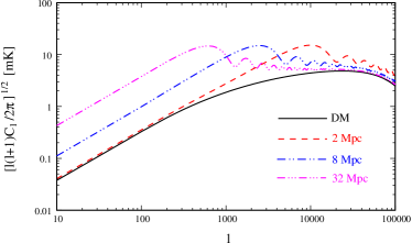
Figure 1: The angular power spectrum of HI brightness temperature fluctuations for different models of the HI distribution assuming $b_{c}=1$ and $\sigma_{p}=0$.

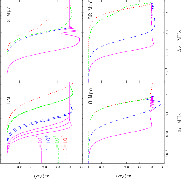
Figure 2: The frequency decorrelation function $\kappa_{l}(\Delta\nu)$ [defined in equation (13)] at $l=10^{2},10^{3},10^{4},10^{5}$. Results are shown for the DM model and the PR model with $b_{c}=1$ and the $R$ values shown in the figure. For the DM model, we show results incorporating the FoG effect using $\sigma_{P}=20\,{\rm and}\,40\,{\rm km/s}$. For each $l$ value $\kappa_{l}(\Delta\nu)$ decreases faster for $\sigma_{P}=0$ and slowest for $\sigma_{P}=40\,{\rm km/s}$. There is a significant change due to the FoG effect only at $l\geq 10^{4}$.

For large bubble size ($R\geq 8~{}\mbox{Mpc}$) the HI signal is dominated by Poisson fluctuations and it is well described through

$$\sqrt{l(l+1)C_{l}}\propto\sqrt{x_{\rm HII}}\,\bar{T}\,\frac{R}{r_{\nu}}\,l$$ (29)

on scales larger than the bubble. At these angular scales the HI signal is substantially enhanced compared to the DM model. For smaller bubble size, the large angle signal is sensitive to the bias $b_{c}$. The signal is very similar to the DM model for $b_{c}=0$ and it is suppressed for higher bias. In all cases (large or small bubble size), the signal is Poisson fluctuation dominated on scales comparable to the bubble size and it peaks at $l\approx\pi r_{\nu}/R$, with no dependence on $b_{c}$. The HI signal traces the dark matter on scales which are much smaller than the bubble size.

We next consider the behavior of $\kappa_{l}(\Delta\nu)$, the frequency decorrelation function shown in Figure 2. For the DM model (upper left panel) where the HI fluctuations trace the dark matter we find that the frequency difference $\Delta\nu$ over which the HI signal remains correlated reduces monotonically with increasing $l$. For example, while for $l=100$ $\kappa_{l}(\Delta\nu)$ falls to $\sim 0.5$ at $\Delta\nu\sim 500\,{\rm KHz}$, it occurs much faster ($\Delta\nu\sim 10\,{\rm KHz}$) for $l=10^{5}$. Beyond the first zero crossing $\kappa_{l}(\Delta\nu)$ becomes negative (anti-correlation) and exhibits a few highly damped oscillations very close to zero. These oscillations arise from the $\cos$ term in equation (21). The change in the behavior of $\kappa_{l}(\Delta\nu)$ for the DM model arising from the FoG effect is also shown in the same panel. Wang & Hu (2005) have proposed that $\sigma_{p}$ is expected to have a value $\sim 30\,{\rm km/s}$ at $z\sim 8$; in view of this, we show results for $\sigma_{p}=20\,{\rm and}\,40\,{\rm km/s}$. We find that there is a discernible change at $l\geq 10^{4}$, and the FoG effect causes the signal to remain correlated for a larger value of $\Delta\nu$. For $\sigma_{p}=20\,{\rm km/s}$, the change is at most $15\%$ for $l=10^{4}$ and around $100\%$ at $l=10^{5}$. Though we have not shown it explicitly, we expect similar changes due to FoG effect in the PR model also.

The patchy reionization model shows distinct departures from the DM model in the behavior of $\kappa_{l}(\Delta\nu)$. This reflects the imprint of the bubble size and the bias on the $\Delta\nu$ dependence. For $R=2\,{\rm Mpc}$ and $b_{c}=1$ (upper right panel) the large $l$ ($l>1000$, comparable to bubble size) behavior is dominated by the Poisson fluctuation of the individual bubbles which makes $\kappa_{l}(\Delta\nu)$ quite distinct from the DM model. Notice that for $l=10^{3}$, $\kappa_{l}(\Delta\nu)$ falls faster than the DM model whereas for $l=10^{4}$ it falls slower than the DM model causing the $l=10^{3}$ and $10^{4}$ curves to nearly overlap. The oscillations seen in $C_{l}$ as a function of $l$ in Figure 1 are also seen in the $\Delta\nu$ dependence of $\kappa_{l}(\Delta\nu)$ at large $l$ ($10^{5}$). The behavior at $l=10^{2}$ is a combination of the dark matter and the ionized bubbles, and is sensitive to $b_{c}$. For $b_{c}=1$, the initial decrease in $\kappa_{l}(\Delta\nu)$ is much steeper than the DM model with a sudden break after which the curve flattens. Figure 3 shows the $b_{c}$ dependence for $l=10^{2}$ and $10^{3}$. The bias dependence is weak for $l=10^{3}$ where the Poisson fluctuations begin to dominate. For $l=10^{2}$, changing $b_{c}$ has a significant affect only near the break in $\kappa_{l}(\Delta\nu)$ leaving much of the curve unaffected. For a smaller bubble size we expect a behavior similar to $R=2{\rm Mpc}$, with the $b_{c}$ dependence being somewhat more pronounced and the Poisson dominated regime starting from a larger value of $l$.

For large bubble size $(R\geq 8{\rm Mpc})$ the large angle HI signal ($l<\pi r_{\nu}/R$) is entirely determined by the Poisson fluctuations where the signal is independent of $l$. This is most clearly seen for $R=8{\rm Mpc}$ where the $\kappa_{l}(\Delta\nu)$ curves for $l=10^{2}$ and $l=10^{3}$ are identical. For both $R=8{\rm Mpc}$ and $32\,{\rm Mpc}$ the large $l$ behavior of $\kappa_{l}(\Delta\nu)$ approaches that of the DM model.

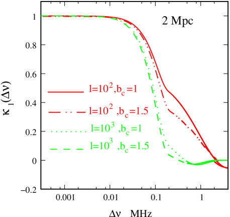
Figure 3: This shows the $b_{c}$ dependence of the frequency decorrelation function $\kappa_{l}(\Delta\nu)$ for the PR model with $R=2\,{\rm Mpc}$.

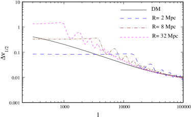
Figure 4: This shows $\Delta\nu_{1/2}$ vs. $l$ for the DM model and the PR model with $b_{c}=1$ for the $R$ values shown in the figure.

In the final part we quantify the frequency difference $\Delta\nu$ across which the HI signal at two different frequencies remain correlated. To be more precise, we study the behavior of $\Delta\nu_{1/2}$ which is defined such that $\kappa_{l}(\Delta\nu_{1/2})=1/2$ ie. the correlation falls to 50% of its peak value at $\Delta\nu=0$. We study this for different angular scales (different $l$) for the various models of HI distribution considered here. The main aim of this exercise is to determine the frequency resolution that would be required to study the HI fluctuations on a given angular scale $l$. Optimally one would like to use a frequency resolution smaller than $\Delta\nu_{1/2}$. A wider frequency channel would combine different uncorrelated signals whereby the signal would cancel out. Further, combining such signals would not lead to an improvement in the signal to noise ratio. Thus it would be fruitful to combine the signal at two different frequencies only as long as they are correlated and not beyond, and we use $\Delta\nu_{1/2}$ to estimate this. The plot of $\Delta\nu_{1/2}$ vs $l$ for the different HI models is shown in Figure 4.

We find that for the DM model $\Delta\nu_{1/2}$ falls monotonically with $l$ and the relation is well approximated by a power law

$$\Delta\nu_{1/2}=\,0.2{\,\rm MHz}\times\left(\frac{l}{10^{3}}\right)^{-0.7}$$ (30)

which essentially says that $\Delta\nu_{1/2}\sim 0.66\,{\rm MHz}$ on $1^{\circ}$ angular scales, $\Delta\nu_{1/2}\sim 0.04\,{\rm MHz}$ on $1^{\prime}$ angular scales and $\Delta\nu_{1/2}\sim 2\,{\rm KHz}$ on $1^{\prime\prime}$ angular scales.

For the PR model, as discussed earlier, $\kappa_{l}(\Delta\nu)$ is $l$ independent on angular scales larger than the bubble size $l<\pi r_{\nu}/R$. As a consequence $\Delta\nu_{1/2}$ also is independent of $l$ and it depends only on the bubble size $R$. This can be well approximated by

$$\Delta\nu_{1/2}\approx 0.04~{}\mbox{MHz}~{}\left(\frac{R}{\mbox{Mpc}}\right)$$ (31)

which given a large value $1.3\,{\rm MHz}$ for $R=32\,{\rm Mpc}$ while it falls below the DM model for $0.08\,{\rm MHz}$ for $R=2\,{\rm Mpc}$. The large $l$ behavior of $\Delta\nu_{1/2}$ approaches the DM model though there are oscillations which persist even at large $l$.

We note that our findings are consistent with the earlier findings of Bharadwaj & Ali (2005) whereas they significantly different from the results of Santos, Cooray & Knox (2005) who assume frequency channels of $1\,{\rm MHz}$ which is too large.

4 Implications for separating signal from Foregrounds

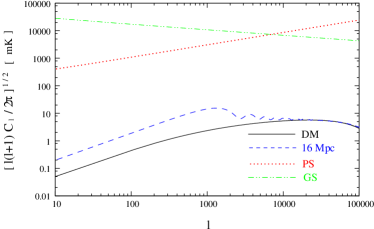
Figure 5: Angular power spectrum $C_{l}(0)$ at $\nu=129\,{\rm MHz}$ for the two most dominant foreground components, the diffuse galactic synchrotron radiation (GS) and the extragalactic point sources (PS) assuming $S_{cut}=0.1\,{\rm mJy}$. The expected signal is also shown for the DM model and the PR model with $R=16\,{\rm Mpc}$.

Astrophysical foregrounds are expected to be several order of magnitude stronger than the 21 cm signal. The MAPS foreground contribution at a frequency $\nu$ can be parametrized as (Santos, Cooray & Knox, 2005)

$$C_{l}(\Delta\nu)=A\left(\frac{\nu_{f}}{\nu}\right)^{\bar{\alpha}}\left(\frac{\nu_{f}}{\nu+\Delta\nu}\right)^{\bar{\alpha}}\left(\frac{1000}{l}\right)^{\beta}I_{l}(\Delta\nu)$$ (32)

where $\nu_{f}=130$ MHz and $\bar{\alpha}$ is the mean spectral index. The actual spectral index varies with line of sight across the sky and this causes the foreground contribution to decorrelate with increasing frequency separation $\Delta\nu$ which is quantified through the foreground frequency decorrelation function $I_{l}(\Delta\nu)$ (Zaldarriaga, Furlanetto & Hernquist, 2004) which has been modeled as

$$I_{l}(\Delta\nu)=\exp\left[-\log_{10}^{2}\left(1+\frac{\Delta\nu}{\nu}\right)/2\xi^{2}\right]\,.$$ (33)

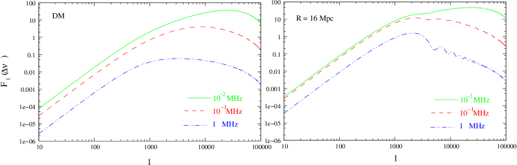
Figure 6: This shows $F_{l}(\Delta\nu)$ (defined in equation 34) for the $\Delta\nu$ values shown in the figure. We consider both the DM model(left panel) and the PR model(right panel).

We consider the two most dominant foreground components namely extragalactic point sources and the diffuse synchrotron radiation from our own galaxy. Point sources above a flux level $S_{cut}$ can be identified in high-resolution images and removed. We assume $S_{cut}=0.1{\rm mJy}$ and adopt the parameter values from Table 1 of Santos, Cooray & Knox (2005) for $A$, $\bar{\alpha}$, $\beta$ and $\xi$. Figure 5 shows the expected $C_{l}(0)$ for the signal and foregrounds. The galactic synchrotron radiation dominates at large angular scales $l<10,000$ while the extragalactic point sources dominate at small angular scales. For all values of $l$, the foregrounds are at least two orders of magnitude larger than the signal.

The foregrounds have a continuum spectra, and the contributions at a frequency separation $\Delta\nu$ are expected to be highly correlated. For $\Delta\nu=1\,{\rm MHz}$, the foreground decorrelation function $I_{l}(\Delta\nu)$ falls by only $2\times 10^{-6}$ for the galactic synchrotron radiation and by $3\times 10^{-5}$ for the point sources. In contrast, the HI decorrelation function $\kappa_{l}(\Delta\nu)$ is nearly constant at very small $\Delta\nu$ and then has a sharp drop well within $1\,{\rm MHz}$, and is largely uncorrelated beyond. This holds the promise of allowing the signal to be separated from the foregrounds. A possible strategy is to cross-correlate different frequency channels of the full data which has both signal and foregrounds, and to use the distinctly different $\Delta\nu$ dependence to separate the signal from the foregrounds (Zaldarriaga, Furlanetto & Hernquist, 2004). An alternate approach is to subtract a best fit continuum spectra along each line of sight (Wang et al., 2006) and then determine the power spectrum. This is expected to be an effective foreground subtraction method in data with very low noise levels. We consider the former approach here, and discuss the implications of our results.

MAPS characterizes the joint $l$ and $\Delta\nu$ dependence which is expected to be different for the signal and the foregrounds. For a fixed $l$, it will be possible to separate the two with relative ease at a frequency separation $\Delta\nu$ if the decrement in the signal $C_{l}(0)[1-\kappa_{l}(\Delta\nu)]$ is more than that of the foregrounds $C_{l}(0)[1-I_{l}(\Delta\nu)]$. Note that because the foregrounds are much stronger than the HI signal, a very small decorrelation of the foreground contribution may cause a decrement in $C_{l}(\Delta\nu)$ which is larger than that due to the signal. We use $F_{l}(\Delta\nu)$ defined as the ratio of the two decrements

$$F_{l}(\Delta\nu)=\frac{\{C_{l}(0)[1-\kappa_{l}(\Delta\nu)]\}_{\rm Signal}}{\{C_{l}(0)[1-I_{l}(\Delta\nu)]\}_{\rm Foregrounds}}$$ (34)

to asses the feasibility of separating the HI signal from the foregrounds. This gives an estimate of the accuracy at which the $\Delta\nu$ dependence of the foreground $C_{l}(\Delta\nu)$ has to be characterized for the signal to be detected. Note we assume that the $\left(\frac{\nu_{f}}{\nu+\Delta\nu}\right)^{\bar{\alpha}}$ term in eq. (32) can be factored out before considering the decrement in the foreground. Figure 6 shows the results for the DM model and the PR model with $R=16\,{\rm Mpc}$. First we note that $F_{l}(\Delta\nu)$ peaks at the angular scales corresponding to $l\sim 10,000$ $(ie.\,2^{{}^{\prime}})$ and the prospects of separating the signal from the foregrounds are most favorable at these scales. A detection will be possible in the range $l>1000$, $\Delta\nu\leq 10{\rm KHz}$ and $l>400$,$\Delta\nu\leq 100{\rm KHz}$ for the DM and PR models respectively provided the $\Delta\nu$ dependence of the foregrounds $C_{l}(\Delta\nu)$ can be characterized with an uncertainty less than order unity. The $l$ and $\Delta\nu$ range would increase if the $\Delta\nu$ dependence of the foreground $C_{l}(\Delta\nu)$ were characterized to $10\%$ accuracy. The largest angular scales ( $l<100$ ) would require an accuracy better than $1\%$ which would possibly set the limit for forthcoming observations.

The angular modes $l=1,000$ and $l=10,000$ correspond to baselines with antenna separations of $\sim 300\,{\rm m}$ and $\sim 3\,{\rm km}$ respectively. This baseline range is quite well covered by the GMRT, and also the forthcoming interferometric arrays. This is possibly the optimal range for a detection. A possible detection strategy would be to use the $\Delta\nu$ behavior of $C_{l}(\Delta\nu)$ in the range where $F_{l}(\Delta\nu)\ll 1$ to characterize the foreground contribution. This can be extrapolated to predict the foreground contribution at small $\Delta\nu$ and any excess relative to this prediction can be interpreted as the HI signal. A very precise determination of the $\Delta\nu$ dependence of the foreground contribution would require a very large $\Delta\nu$ range in the region where $F_{l}(\Delta\nu)\ll 1$, and a bandwidth of $\sim 10{\rm MHz}$ would be appropriate. On the other hand, at $l\sim 10,000$ the HI $C_{l}(\Delta\nu)$ decorrelates within $\sim 50{\rm KHz}$ [or equivalently $F_{l}(\Delta\nu)$ shows a considerable drop between $10\,{\rm KHz}$ and $100\,{\rm KHz}$, see Figure 6], and it would be desirable to have a frequency resolution better than $\sim 10{\rm KHz}$ to optimally differentiate between the signal and the foregrounds. A lower resolution of $\sim 20\,{\rm KHz}$ would possibly suffice at $l\sim 1,000$, particularly if the PR model holds.

Appendix A Calculation of the angular power spectrum $C_{l}(\nu_{1},\nu_{2})$

In this section, we present the details of the calculation for the 21 cm angular power spectrum $C_{l}(\nu_{1},\nu_{2})$. The first step would be to calculate the spherical harmonic component $a_{lm}$ of the brightness temperature $T(\nu,{\bf\hat{n}})$. Using the expression (6) for $\tilde{\eta}_{\rm HI}\left({\bf k}\right)$ in equation (LABEL:eq:a_lm), the expression for $a_{lm}$ can be written as

$$a_{lm}(\nu) = \bar{T}~{}\bar{x}_{\rm HI}\int{\rm d}\Omega~{}Y^{*}_{lm}({\bf\hat{n}})~{}\int\frac{{\rm d}^{3}k}{(2\pi)^{3}}$$ (35)

$$\times \left[\Delta_{\rm HI}({\bf k})+({\bf\hat{n}\cdot\hat{k}})^{2}\Delta({\bf k})\right]{\rm e}^{-{\rm i}kr_{\nu}({\bf\hat{k}\cdot\hat{n}})}$$

which then essentially involves solving angular integrals of the forms $\int{\rm d}\Omega~{}Y^{*}_{lm}~{}{\rm e}^{-{\rm i}kr_{\nu}({\bf\hat{k}\cdot\hat{n}})}$ and $\int{\rm d}\Omega~{}Y^{*}_{lm}~{}({\bf\hat{n}\cdot\hat{k}})^{2}{\rm e}^{-{\rm i}kr_{\nu}({\bf\hat{k}\cdot\hat{n}})}$ respectively. Expanding the term ${\rm e}^{-{\rm i}kr_{\nu}({\bf\hat{k}\cdot\hat{n}})}$ in terms of spherical Bessel functions $j_{l}(kr_{\nu})$, one can show that

$$\int{\rm d}\Omega~{}Y^{*}_{lm}({\bf\hat{n}})~{}{\rm e}^{-{\rm i}kr_{\nu}({\bf\hat{k}\cdot\hat{n}})}=4\pi(-{\rm i})^{l}j_{l}(kr_{\nu})Y^{*}_{lm}({\bf\hat{k}})$$ (36)

Differentiating the above equation with respect to $kr_{\nu}$ twice

$$\int{\rm d}\Omega~{}({\bf\hat{k}\cdot\hat{n}})^{2}~{}Y^{*}_{lm}({\bf\hat{n}})~{}{\rm e}^{-{\rm i}kr_{\nu}({\bf\hat{k}\cdot\hat{n}})}=-4\pi(-{\rm i})^{l}~{}j^{\prime\prime}_{l}(kr_{\nu})Y^{*}_{lm}({\bf\hat{k}})$$ (37)

where $j^{\prime\prime}_{l}(x)$ is the second derivative of $j_{l}(x)$ with respect to its argument, and can be obtained through the recursion relation

$$(2l+1)j^{\prime\prime}_{l}(x)\!\!\!\!\! = \!\!\!\!\!\frac{l(l-1)}{2l-1}j_{l-2}(x)-\left[\frac{l^{2}}{2l-1}+\frac{(l+1)^{2}}{2l+3}\right]j_{l}(x)$$ (38)

$$+ \!\!\!\!\!\frac{(l+1)(l+2)}{2l+3}j_{l+2}(x)$$

So the final expression of $a_{lm}$ is given by

$$a_{lm}(\nu) = 4\pi\bar{T}~{}\bar{x}_{\rm HI}(-{\rm i})^{l}~{}\int\frac{{\rm d}^{3}k}{(2\pi)^{3}}Y^{*}_{lm}({\bf\hat{k}})$$ (39)

$$\times \left[\Delta_{\rm HI}({\bf k})j_{l}(kr_{\nu})-\Delta({\bf k})j^{\prime\prime}_{l}(kr_{\nu})\right]$$

The next step is to calculate the the power spectrum $C_{l}(\nu_{1},\nu_{2})\equiv\langle a_{lm}(\nu_{1})~{}a^{*}_{lm}(\nu_{2})\rangle$. The corresponding expression is then given by

$$C_{l}(\nu_{1},\nu_{2})\!\!\!\!\! = \!\!\!\!\!(4\pi)^{2}\bar{T}(z_{1})\bar{T}(z_{2})~{}\bar{x}_{\rm HI}(z_{1})\bar{x}_{\rm HI}(z_{2})$$

$$\times \!\!\!\!\!\int\frac{{\rm d}^{3}k_{1}}{(2\pi)^{3}}\int\frac{{\rm d}^{3}k_{2}}{(2\pi)^{3}}Y^{*}_{lm}({\bf\hat{k}_{1}})Y_{lm}({\bf\hat{k}_{2}})$$

$$\times \!\!\!\!\!\left\langle\left[\Delta_{\rm HI}(z_{1},{\bf k_{1}})j_{l}(k_{1}r_{\nu_{1}})-\Delta(z_{1},{\bf k_{1}})j^{\prime\prime}_{l}(k_{1}r_{\nu_{1}})\right]\right.$$

$$\times \!\!\!\!\!\left.\left[\Delta^{*}_{\rm HI}(z_{2},{\bf k_{2}})j_{l}(k_{2}r_{\nu_{2}})-\Delta^{*}(z_{2},{\bf k_{2}})j^{\prime\prime}_{l}(k_{2}r_{\nu_{2}})\right]\right\rangle$$

where we have put back the redshift-dependence into the expressions for clarity. Now note that we would mostly be interested in cases where $\nu_{2}-\nu_{1}\equiv\Delta\nu\ll\nu_{1}$. In such cases, one can safely assume $\bar{T}(z_{2})\approx\bar{T}(z_{1})$ and $\bar{x}_{\rm HI}(z_{2})\approx\bar{x}_{\rm HI}(z_{1})$. Furthermore, the terms involving the ensemble averages of the form $\langle\Delta\Delta^{*}\rangle$ can be approximated as $\langle\Delta(z_{1},{\bf k_{1}})\Delta^{*}(z_{2},{\bf k_{2}})\rangle\approx(2\pi)^{3}\delta_{D}({\bf k_{1}-k_{2}})P(z_{1},k_{1})$ and similarly for terms involving $\Delta_{\rm HI}$. We can then use the Dirac delta function $\delta_{D}({\bf k_{1}-k_{2}})$ to compute the ${\bf k_{2}}$-integral, and thus can write the angular power spectrum as

$$C_{l}(\Delta\nu)\!\!\!\!\! \equiv \!\!\!\!\!C_{l}(\nu,\nu+\Delta\nu)$$ (41)

$$= \!\!\!\!\!(4\pi)^{2}~{}\bar{T}^{2}~{}\bar{x}^{2}_{\rm HI}\int\frac{{\rm d}^{3}k_{1}}{(2\pi)^{3}}Y^{*}_{lm}({\bf\hat{k}_{1}})Y_{lm}({\bf\hat{k}_{1}})$$

$$\times \!\!\!\!\!\left[j_{l}(kr_{\nu})j_{l}(kr_{\nu_{2}})P_{\Delta^{2}_{\rm HI}}(k)\right.$$

$$- \!\!\!\!\!\{j_{l}(kr_{\nu})j^{\prime\prime}_{l}(kr_{\nu_{2}})+j_{l}(kr_{\nu_{2}})j^{\prime\prime}_{l}(kr_{\nu})\}P_{\Delta_{\rm HI}}(k)$$

$$+ \!\!\!\!\!\left.j^{\prime\prime}_{l}(kr_{\nu})j^{\prime\prime}_{l}(kr_{\nu_{2}})P(k)\right]$$

Using the normalization property of the spherical harmonics $\int{\rm d}{\bf{\hat{n}}}|Y_{lm}({\bf\hat{n}})|^{2}=1$, one can carry out the angular integrals in the above expression, and hence obtain the final result (2.2) as quoted in the main text.

Appendix B Correspondence between all-sky and flat-sky power spectra

As discussed in section 2.3, we shall mostly be interested in very small angular scales, which corresponds to $l\gg 1$. For high values of $l$, it is most useful to work in the flat-sky approximation, where a small portion of the sky can be approximated by a plane. Then the unit vector ${\bf\hat{n}}$ towards the direction of observation can be decomposed into ${\bf\hat{n}}={\bf m}+\boldsymbol{\theta}$, where ${\bf m}$ is a vector towards the center of the field of view and $\boldsymbol{\theta}$ is a two-dimensional vector in the plane of the sky.

Without loss of generality, let us now consider a small region around the pole $\theta\to 0$. In that case the vector $\boldsymbol{\theta}$ can be treated as a Cartesian vector with components $\{\theta\cos\phi,\theta\sin\phi\}$. This holds true for any two-dimensional vector on the sky, in particular ${\bf U}=\{U\cos\phi_{U},U\sin\phi_{U}\}$. Then the spherical harmonic components of $T(\nu,{\bf\hat{n}})$ [defined in equation (LABEL:eq:a_lm)] can be written as

$$a_{lm}(\nu)\approx\int{\rm d}\boldsymbol{\theta}~{}Y^{*}_{lm}(\theta,\phi)~{}T(\nu,{\bf\hat{n}})$$ (42)

where we have replaced $\int{\rm d}\Omega\rightarrow\int{\rm d}\boldsymbol{\theta}$. Now use the expansion

$${\rm e}^{-2\pi{\rm i}{\bf U\cdot}\boldsymbol{\theta}}=\sum_{m}(-{\rm i})^{m}J_{m}(2\pi U\theta){\rm e}^{{\rm i}m(\phi_{U}-\phi)}$$ (43)

where $J_{m}(x)$ is the ordinary Bessel function. Further, we use the approximation for spherical harmonics

$$Y_{lm}(\theta,\phi)~{}^{\approx}_{\theta\to 0}~{}J_{m}(l\theta)\sqrt{\frac{l}{2\pi}}~{}{\rm e}^{{\rm i}m\phi}$$ (44)

to write

$${\rm e}^{-2\pi{\rm i}{\bf U\cdot}\boldsymbol{\theta}}\approx\sqrt{\frac{1}{U}}~{}\sum_{m}(-{\rm i})^{m}Y^{*}_{2\pi U,m}(\theta,\phi){\rm e}^{-{\rm i}m\phi_{U}}$$ (45)

Then the two-dimensional Fourier transform of the brightness temperature [defined in equation (16)] will be

$$\tilde{T}(\nu,{\bf U})\!\!\!\!\! = \!\!\!\!\!\int{\rm d}\boldsymbol{\theta}~{}{\rm e}^{-2\pi{\rm i}{\bf U\cdot}\boldsymbol{\theta}}~{}T(\nu,{\bf\hat{n}})$$ (46)

$$\approx \!\!\!\!\!\sqrt{\frac{1}{U}}~{}\sum_{m}(-{\rm i})^{m}{\rm e}^{-{\rm i}m\phi_{U}}~{}\int{\rm d}\boldsymbol{\theta}~{}Y^{*}_{2\pi U,m}(\theta,\phi)~{}T(\nu,{\bf\hat{n}})$$

$$= \!\!\!\!\!\sqrt{\frac{1}{U}}~{}\sum_{m}(-{\rm i})^{m}{\rm e}^{-{\rm i}m\phi_{U}}~{}a_{2\pi U,m}(\nu)$$

where we have used the expression (42) for $a_{lm}$ in the last part. This gives a relation between the flat-sky Fourier transform $\tilde{T}(\nu,{\bf U})$ and and its the full-sky equivalent $a_{lm}(\nu)$.

Using the above relation, we can calculate the power spectrum

$$\langle\tilde{T}(\nu_{1},{\bf U})\tilde{T}^{*}(\nu_{2},{\bf U^{\prime}})\rangle\!\!\!\!\! \approx \!\!\!\!\!\sqrt{\frac{1}{UU^{\prime}}}~{}\sum_{mm^{\prime}}(-{\rm i})^{m-m^{\prime}}{\rm e}^{-{\rm i}m\phi_{U}}~{}{\rm e}^{{\rm i}m^{\prime}\phi_{U^{\prime}}}$$ (47)

$$\times \!\!\!\!\!\langle a_{2\pi U,m}(\nu_{1})a^{*}_{2\pi U^{\prime},m^{\prime}}(\nu_{2})\rangle$$

Use the definition $\langle a_{lm}(\nu_{1})a^{*}_{l^{\prime}m^{\prime}}(\nu_{2})\rangle=C_{l}\delta_{ll^{\prime}}\delta_{mm^{\prime}}$ and the property

$$\sum_{m}{\rm e}^{-{\rm i}m(\phi_{U}-\phi_{U^{\prime}})}=2\pi\delta^{(1)}_{D}(\phi_{U}-\phi_{U^{\prime}})$$ (48)

to obtain

$$\langle\tilde{T}(\nu_{1},{\bf U})\tilde{T}^{*}(\nu_{2},{\bf U^{\prime}})\rangle=2\pi~{}C_{2\pi U}(\nu_{1},\nu_{2})~{}\frac{\delta_{UU^{\prime}}}{U}~{}\delta^{(1)}_{D}(\phi_{U}-\phi_{U^{\prime}})$$ (49)

The last step involves writing the right hand side of the above equation in terms of the two-dimensional Dirac delta function, which follows from the expansion

$$\delta^{(2)}_{D}({\bf U-U^{\prime}})=\int{\rm d}\boldsymbol{\theta}~{}{\rm e}^{-2\pi{\rm i}{\bf(U-U^{\prime})\cdot}\boldsymbol{\theta}}$$ (50)

The exponentials can be written in terms of the spherical harmonics using equation (45):

$$\delta^{(2)}_{D}({\bf U-U^{\prime}})\!\!\!\!\! \approx \!\!\!\!\!\int{\rm d}\boldsymbol{\theta}~{}\sqrt{\frac{1}{UU^{\prime}}}\sum_{mm^{\prime}}(-{\rm i})^{m-m^{\prime}}$$

$$\times \!\!\!\!\!Y^{*}_{2\pi U,m}(\theta,\phi)Y_{2\pi U^{\prime},m^{\prime}}(\theta,\phi){\rm e}^{-{\rm i}m\phi_{U}}{\rm e}^{{\rm i}m^{\prime}\phi_{U^{\prime}}}$$

Finally use the orthonormality property of spherical harmonics $\int{\rm d}\boldsymbol{\theta}Y^{*}_{lm}(\theta,\phi)Y_{l^{\prime}m^{\prime}}(\theta,\phi)=\delta_{ll^{\prime}}\delta_{mm^{\prime}}$ and the relation (48) to obtain

$$\delta^{(2)}_{D}({\bf U-U^{\prime}})=2\pi~{}\frac{\delta_{UU^{\prime}}}{U}\delta_{D}(\phi_{U}-\phi_{U^{\prime}})$$ (52)

Putting the above relation into (49), we obtain equation (20) used in the final text.

References

- Ali, Bharadwaj and Pandey (2005) Ali, S. S., Bharadwaj, S., & Pandey, B. 2005, MNRAS, 363, 251
- Ali, Bharadwaj and Pandey (2006) Ali, S. S., Bharadwaj, S., & Pandey, S. K. 2006, MNRAS, 366, 213
- Alvarez et al. (2006) Alvarez, M. A., Shapiro, P. R., Ahn, K. & Iliev, I. T. 2006, astro-ph/0604447
- Ballinger et al. (1996) Ballinger, W. E., Peacock, J. A. , Heavens , A. F. 1996, MNRAS, 282 , 877
- Barkana & Loeb (2001) Barkana R. & Loeb A., 2001, Phys.Rep., 349, 125
- Becker et al. (2001) Becker, R.H., et al., 2001, AJ, 122, 2850
- Bharadwaj, Nath & Sethi (2001) Bharadwaj S., Nath B. & Sethi S.K. 2001, JApA.22,21
- Bharadwaj & Sethi (2001) Bharadwaj, S. & Sethi, S. K. 2001, JApA, 22, 293
- Bharadwaj & Pandey (2003) Bharadwaj, S. & Pandey, S. K. 2003, JApA, 24, 23
- Bharadwaj & Srikant (2004) Bharadwaj, S., & Srikant, P. S. 2004, JApJ, 25, 67
- Bharadwaj & Ali (2004) Bharadwaj, S., & Ali, S. S. 2004, MNRAS, 352, 142
- Bharadwaj & Ali (2005) Bharadwaj, S., & Ali, S. S. 2005, MNRAS, 356, 1519
- Bharadwaj & Pandey (2005) Bharadwaj, S., & Pandey, S. K. 2005, MNRAS, 358, 968
- Bunn & White ((1996)) Bunn E.F., & White M., 1996 ,ApJ,460,1071
- Carilli (2006) Carilli, C. L. 2006, New Astronomy Review, 50, 162
- Chen & Miralda-Escude (2004) Chen, X. & Miralda-Escude,J., 2004, ApJ, 602, 1
- Choudhury & Ferrara (2006a) Choudhury T. R., Ferrara A., Preprint: astro-ph/0603149, 2006a
- Choudhury & Ferrara (2006b) Choudhury T. R., Ferrara A. 2006b, MNRAS, 371, L55
- Ciardi & Madau (2003) Ciardi, B.& Madau, P. 2003, ApJ, 596, 1
- Colombo (2004) Colombo, L. P. L., 2004, JCAP, 3, 3
- Cooray & Furlanetto (2004) Cooray, A., & Furlanetto, S. R. 2004, ApJL, 606, L5
- Cooray & Furlanetto (2005) Cooray, A., & Furlanetto, S. R. 2005, MNRAS, 359, L47
- Cooray (2005) Cooray, A. 2005, MNRAS, 363, 1049
- DiMatteo. et al. (2004) Di Matteo, T., Ciardi, B., & Miniati, F. 2004, MNRAS, 355, 1053
- DiMatteo. et al. (2002) DiMatteo,T., Perna R., Abel,T., Rees,M.J. 2002, ApJ, 564, 576
- Fan, Carilli & Keating (2006) X. Fan, C. L. Carilli, and B. Keating, Preprint: astro-ph/0602375, 2006.
- Fan et al. (2002) Fan,X., et al. 2002, AJ, 123, 1247
- Furlanetto, Sokasian & Hernquist (2004) Furlanetto, S. R., Sokasian, A., & Hernquist, L. 2004, MNRAS, 347, 187
- Furlanetto, Zaldarriaga & Hernquist (2004a) Furlanetto, S. R., Zaldarriaga, M., & Hernquist, L. 2004a, ApJ, 613, 1
- Furlanetto, Zaldarriaga & Hernquist (2004b) Furlanetto, S. R., Zaldarriaga, M., & Hernquist, L. 2004b, ApJ, 613, 16
- Furlanetto, McQuinn & Hernquist (2006) Furlanetto, S. R., McQuinn, M., & Hernquist, L. 2006, MNRAS, 365, 115
- Furlanetto et al. (2006) Furlanetto, S. R., Oh, S. P., & Briggs, F. H. 2006, Physics Report, 433, 181
- Gnedin & Ostriker (1997) Gnedin, N. Y. & Ostriker, J. P,1997,ApJ,486,581
- Gnedin & Shaver (2004) Gnedin, N. Y., & Shaver, P. A. 2004, ApJ, 608, 611
- Haiman & Holder (2003) Haiman, Z. & Holder, G.P. 2003,ApJ,595,1
- He et al. (2004) He, P., Liu, J., Feng, L.-L., Bi, H.-G., & Fang, L.-Z. 2004, ApJ, 614, 6
- Hogan & Rees (1979) Hogan, C. J. & Rees, M. J., 1979, MNRAS,188,791
- Hu & Holder (2003) Hu, W., & Holder, G. P. 2003, PRD, 68, 023001
- Hui & Haiman (2003) Hui, L., & Haiman, Z., 2003, ApJ,596,9
- Iliev et al. (2002) Iliev, I.T., Shapiro, P.R., Farrara, A., Martel, H. 2002, ApJ, 572, L123
- Iliev et al. (2003) Iliev, I.T., Scannapieco, E., Martel, H., Shapiro, P.R. 2003, MNRAS, 341, 81
- Iliev et al. (2005) Iliev, I.T., Mellema, G., Pen, Ue-Li., Merz, H., Shapiro, P.R., Alvarez, M.A., 2005, MNRAS submitted, astro-ph/0512187
- Kaplinghat et al. (2003) Kaplinghat, M., Chu, M., Haiman, Z., Holder, G.P., Knox, L., & Skordis, C. 2003, ApJL, 583, 24
- Loeb & Zaldarriaga (2004) Loeb, A., & Zaldarriaga, M. 2004, PRL, 92, 211301
- Mcquinn et al. (2005) McQuinn, M., Zahn, O., Zaldarriaga, M., Hernquist, L., Furlanetto, S.R., 2005, astro-ph/0512263
- Madau, Meiksin & Rees ((1997)) Madau P., Meiksin A. & Rees, M. J.,1997,ApJ,475,429
- Mellema et al. (2006) Mellema G., Iliev I.T., Pen Ue-Li.,& Shapiro P.R., 2006, astro-ph/0603518
- Miralda-Escude (2003) Miralda-Escude, J., 2003, Science 300, 1904-1909
- Morales & Hewitt (2004) Morales, M. F., & Hewitt, J. 2004, ApJ, 615, 7
- Oh (1999) Oh, S. P. 1999, ApJ, 527, 16
- Oh & Mack (2003) Oh, S.P., & Mack,K.J., 2003, MNRAS, 346, 871
- Page et al. (2006) Page L. et al., 2006, Preprint: astro-ph/0603450
- Peacock (1999) Peacock J.A., 1999, Cosmological Physics, Cambridge Univ. Press, Cambridge, pp.517
- Salvaterra et al. (2005) Salvaterra, R., Ciardi, B., Ferrara, A., & Baccigalupi, C. 2005, MNRAS, 360, 1063
- Santos, Cooray & Knox (2005) Santos, M. G., Cooray, A., & Knox, L. 2005, ApJ, 625, 575
- Scott & Rees (1990) Scott D. & Rees, M. J., 1990, MNRAS,247,510
- Sethi (2005) Sethi, S. K., 2005, MNRAS, 363, 818
- Shaver et al. (1999) Shaver, P. A., Windhorst, R, A., Madau, P.& de Bruyn, A. G., 1999, Astron. & Astrophys.,345,380
- Sheth (1996) Sheth, R. 1996, MNRAS, 279, 1310
- Spergel et al. (2006) Spergel, D. N.,et al. 2006,astro-ph/0603449
- Sunyaev and Zeldovich (1972) Sunyaev, R. A. & Zeldovich, Ya. B., 1972,Astron. & Astrophys,22,189
- Swarup et al. (1991) Swarup G., Ananthakrishnan S., Kapahi V.K., Rao A.P., Subramanya C.R., Kulkarni V.K.,1991 Curr.Sci.,60,95
- Tozzi et al. (2000) Tozzi.P., Madau.P., Meiksin. A., Rees,M.J.,2000,ApJ,528,597
- Wang & Hu (2005) Wang, X. & Hu, W. 2005, astro-ph/0511141
- Wang et al. (2006) Wang, X., Tegmark, M., Santos, M. G., & Knox, L. 2006, ApJ, 650, 529
- Wyithe & Loeb (2004) Wyithe, J. S. B., Loeb, A. 2004, Nature, 432, 194
- Zaldarriaga, Furlanetto & Hernquist (2004) Zaldarriaga, M., Furlanetto, S. R., & Hernquist, L. 2004, ApJ, 608, 622