Magnetic fields, strings and cosmology

1 Half a century of large-scale magnetic fields

1.1 A premise

The content of the present contribution is devoted to large-scale magnetic fields whose origin, evolution and implications constitute today a rather intriguing triple point in the phase diagram of physical theories. Indeed, sticking to the existing literature (and refraining from dramatic statements on the historical evolution of theoretical physics) it appears that the subject of large-scale magnetization thrives and prosper at the crossroad of astrophysics, cosmology and theoretical high-energy physics.

Following the kind invitation of Jnan Maharana and Maurizio Gasperini, I am delighted to contribute to this set of lectures whose guideline is dictated by the inspiring efforts of Gabriele Veneziano in understanding the fundamental forces of Nature. My voice joins the choir of gratitude proceeding from the whole physics community for the novel and intriguing results obtained by Gabriele through the various stages of his manifold activity. I finally ought to convey my personal thankfulness for the teachings, advices and generous clues received during the last fifteen years.

1.2 Length scales

The typical magnetic field strengths, in the Universe, range from few $\mu{\mathrm{G}}$ (in the case of galaxies and clusters), to few G (in the case of planets, like the earth or Jupiter) and up to $10^{12}{\mathrm{G}}$ in neutron stars. Magnetic fields are not only observed in planets and stars but also in the interstellar medium, in the intergalactic medium and, last but not least, in the intra-cluster medium.

Magnetic fields whose correlation length is larger than the astronomical unit ( $1\,{\rm AU}=1.49\times 10^{13}{\rm cm}$) will be named large-scale magnetic fields. In fact, magnetic fields with approximate correlation scale comparable with the earth-sun distance are not observed (on the contrary, both the magnetic field of the sun and the one of the earth have a clearly distinguishable localized structure). Moreover, in magnetohydrodynamics (MHD), the magnetic diffusivity scale (i.e. the scale below which magnetic fields are diffused because of the finite value of the conductivity) turns out to be, amusingly enough, of the order of the AU.

1.3 The early history

In the forties large-scale magnetic field had no empirical evidence. For instance, there was no evidence of magnetic fields associated with the galaxy as a whole with a rough correlation scale of $30\mathrm{kpc}$. More specifically, the theoretical situation can be summarized as follows. The seminal contributions of H. Alfvén alv1 convinced the community that magnetic fields can have a very large life-time in a highly conducting plasma. Later on, in the seventies, Alfvén will be awarded by the Nobel prize “for fundamental work and discoveries in magnetohydrodynamics with fruitful applications in different parts of plasma physics”.

Using the discoveries of Alfvén, Fermi fermi postulated, in 1949, the existence of a large-scale magnetic field permeating the galaxy with approximate intensity of $\mu$ G and, hence, in equilibrium with the cosmic rays

Alfvén alv2 did not react positively to the proposal of Fermi, insisting, in a somehow opposite perspective, that cosmic rays are in equilibrium with stars and disregarding completely the possibility of a galactic magnetic field. Today we do know that this may be the case for low-energy cosmic rays but certainly not for the most energetic ones around, and beyond, the knee in the cosmic ray spectrum.

At the historical level it is amusing to notice that the mentioned controversy can be fully understood from the issue $75$ of Physical Review where it is possible to consult the paper of Fermi fermi , the paper of Alfvén alv2 and even a paper by R. D. Richtmyer and E. Teller alv3 supporting the views and doubts of Alfvén.

In 1949 Hiltner hiltner and, independently, Hall hall observed polarization of starlight which was later on interpreted by Davis and Greenstein davis as an effect of galactic magnetic field aligning the dust grains.

According to the presented chain of events it is legitimate to conclude that

• the discoveries of Alfvén were essential in the Fermi proposal who was pondering on the origin of cosmic rays in 1938 before leaving Italy because of the infamous fascist legislation;

• the idea that cosmic rays are in equilibrium with the galactic magnetic fields (and hence that the galaxy possess a magnetic field) was essential in the correct interpretation of the first, fragile, optical evidence of galactic magnetization.

The origin of the galactic magnetization, according to fermi , had to be somehow primordial. It should be noticed, for sake of completeness, that the observations of Hiltner hiltner and Hall hall took place from November 1948 to January 1949. The paper of Fermi fermi was submitted in January 1949 but it contains no reference to the work of Hiltner and Hall. This indicates the Fermi was probably not aware of these optical measurements.

The idea that large-scale magnetization should somehow be the remnant of the initial conditions of the gravitational collapse of the protogalaxy idea was further pursued by Fermi in collaboration with S. Chandrasekar fermi2 ; fermi3 who tried, rather ambitiously, to connect the magnetic field of the galaxy to its angular momentum.

1.4 The middle ages

In the fifties various observations on polarization of Crab nebula suggested that the Milky Way is not the only magnetized structure in the sky. The effective new twist in the observations of large-scale magnetic fields was the development (through the fifties and sixties) of radio-astronomical techniques. From these measurements, the first unambiguous evidence of radio-polarization from the Milky Way (MW) was obtained (see wiel and references therein for an account of these developments).

It was also soon realized that the radio-Zeeman effect (counterpart of the optical Zeeman splitting employed to determine the magnetic field of the sun) could offer accurate determination of (locally very strong) magnetic fields in the galaxy. The observation of Lyne and Smith lyne that pulsars could be used to determine the column density of electrons along the line of sight opened the possibility of using not only synchrotron emission as a diagnostic of the presence of a large-scale magnetic field, but also Faraday rotation. For a masterly written introduction to pulsar physics the reader may consult the book of Lyne and Smith lynebook .

In the seventies all the basic experimental tools for the analysis of galactic and extra-galactic magnetic fields were ready. Around this epoch also extensive reviews on the experimental endeavors started appearing and a very nice account could be found, for instance, in the review of Heiles heiles .

It became gradually evident in the early eighties, that measurements of large-scale magnetic fields in the MW and in the external galaxies are two complementary aspects of the same problem. While MW studies can provide valuable informations concerning the local structure of the galactic magnetic field, the observation of external galaxies provides the only viable tool for the reconstruction of the global features of the galactic magnetic fields.

Since the early seventies, some relevant attention has been paid not only to the magnetic fields of the galaxies but also to the magnetic fields of the clusters. A cluster is a gravitationally bound system of galaxies. The local group (i.e. our cluster containing the MW, Andromeda together with other fifty galaxies) is an irregular cluster in the sense that it contains fewer galaxies than typical clusters in the Universe. Other clusters (like Coma, Virgo) are more typical and are then called regular or Abell clusters. As an order of magnitude estimate, Abell clusters can contain $10^{3}$ galaxies.

1.5 New twists

In the nineties magnetic fields have been measured in single Abell clusters but around the turn of the century these estimates became more reliable thanks to improved experimental techniques. In order to estimate magnetic fields in clusters, an independent knowledge of the electron density along the line of sight is needed. Recently Faraday rotation measurements obtained by radio telescopes (like VLA ) have been combined with independent measurements of the electron density in the intra-cluster medium. This was made possible by the maps of the x-ray sky obtained with satellites measurements (in particular ROSAT ). This improvement in the experimental capabilities seems to have partially settled the issue confirming the measurements of the early nineties and implying that also clusters are endowed with a magnetic field of $\mu$G strength which is not associated with individual galaxies gov ; fer .

While entering the new millennium the capabilities of the observers are really confronted with a new challenge: the possibility that also superclusters are endowed with their own magnetic field. Superclusters are (loosely) gravitationally bound systems of clusters. An example is the local supercluster formed by the local group and by the VIRGO cluster. Recently a large new sample of Faraday rotation measures of polarized extragalactic sources has been compared with galaxy counts in Hercules and Perseus-Pisces (two nearby superclusters) kro2 . First attempts to detect magnetic fileds associated with superclusters have been reported kro3 . A cautious and conservative approach suggests that these fragile evidences must be corroborated with more conclusive observations (especially in the light of the, sometimes dubious, independent determination of the electron density ). However it is not excluded that as the nineties gave us a firmer evidence of cluster magnetism, the new millennium may give us more solid understanding of supercluster magnetism. In the present historical introduction various experimental techniques have been swiftly mentioned. A more extensive introductory description of these techniques can be found in f1 .

1.6 Hopes for the future

The hope for the near future is connected with the possibility of a next generation radio-telescope. Along this line the SKA (Square Kilometer Array) has been proposed fer (see also SKA ). While the technical features of the instrument cannot be thoroughly discussed in the present contribution, it suffices to notice that the collecting area of the instrument, as the name suggest, will be of $10^{6}\,{\rm m}^{2}$. The specifications for the SKA require an angular resolution of $0.1$ arcsec at $1.4$ GHz, a frequency capability of $0.1$–$25$ GHz, and a field of view of at least $1\,{\rm deg}^{2}$ at $1.4$ GHz SKA . The number of independent beams is expected to be larger than $4$ and the number of instantaneous pencil beams will be roughly 100 with a maximum primary beam separation of about $100$ $\mathrm{deg}$ at low frequencies (becoming $1$ $\mathrm{deg}$ at high frequencies, i.e. of the order of $1$ GHz). These specifications will probably allow full sky surveys of Faraday Rotation.

The frequency range of SKA is rather suggestive if we compare it with the one of the Planck experiment planck . Planck will operate in $9$ frequency channels from $30$ to, approximately, $900$ GHz. While the three low-frequency channels (from $30$ to $70$ GHz) are not sensitive to polarization the six high-frequency channels (between $100$ and $857$ GHZ) will be definitely sensitive to CMB polarization. Now, it should be appreciated that the Faraday rotation signal decreases with the frequency $\nu$ as $\nu^{-2}$. Therefore, for lower frequencies the Faraday Rotation signal will be larger than in the six high-frequency channels. Consequently it is legitimate to hope for a fruitful interplay between the next generation of SKA-like radio-telescopes and CMB satellites. Indeed, as suggested above, the upper branch of the frequency capability of SKA almost overlaps with the lower frequency of Planck so that possible effects of large-scale magnetic fields on CMB polarization could be, with some luck, addressed with the combined action of both instruments. In fact, the same mechanism leading to the Faraday rotation in the radio leads to a Faraday rotation of the CMB provided the CMB is linearly polarized. These considerations suggest, as emphasized in a recent topical review, that CMB anisotropies are germane to several aspects of large-scale magnetization maxcqg . The considerations reported so far suggest that during the next decade the destiny of radio-astronomy and CMB physics will probably be linked together and not only for reasons of convenience.

1.7 Few burning questions

In this general and panoramic view of the history of the subject we started from the relatively old controversy opposing E. Fermi to H. Alfvén with the still uncertain but foreseeable future developments. While the nature of the future developments is inextricably connected with the advent of new instrumental capabilities, it is legitimate to remark that, in more than fifty years, magnetic fields have been detected over scales that are progressively larger. From the historical development of the subject a series of questions arises naturally:

• what is the origin of large-scale magnetic fields?

• are magnetic fields primordial as assumed by Fermi more than fifty years ago?

• even assuming that large-scale magnetic fields are primordial, is there a theory for their generation?

• is there a way to understand if large-scale magnetic fields are really primordial?

In what follows we will not give definite answers to these important questions but we shall be content of outlining possible avenues of new developments.

The plan of the present lecture will be the following. In Sect. 2 the main theoretical problems connected with the origin of large-scale magnetic fields will be discussed. In Sect.  3 the attention will be focused on the problem of large-scale magnetic field generation in the framework of string cosmological model, a subject where the pre-big bang model, in its various incarnations, plays a crucial rôle. But, finally, large-scale magnetic fields are really primordial? Were they really present prior to matter-radiation equality? A modest approach to these important questions suggests to study the physics of magnetized CMB anisotropies which will be introduced, in its essential lines, in Sect. 4. The concluding remarks are collected in Sect.  5.

2 Magnetogenesis

While in the previous Section the approach has been purely historical, the experimental analysis of large-scale magnetic fields prompts a collection of interesting theoretical problems. They can be summarized by the following chain of evidences (see also f1 ):

• In spiral galaxies magnetic fields follow the orientation of the spiral arms, where matter is clustered because of differential rotation. While there may be an asymmetry in the intensities of the magnetic field in the northern and southern emisphere (like it happens in the case of the Milky Way) the typical strength is in the range of the $\mu$ G.

• Locally magnetic fields may even be in the $\mathrm{mG}$ range and, in this case, they may be detected through Zeeman splitting techniques.

• In spiral galaxies the magnetic field is predominantly toroidal with a poloidal component present around the nucleus of the galaxy and extending for, roughly, $100$ pc.

• The correlation scale of the magnetic field in spirals is of the order of $30$ kpc.

• In elliptical galaxies magnetic fields have been measured at the $\mu$ G level but the correlation scale is shorter than in the case of spirals: this is due to the different evolutionary history of elliptical galaxies and to their lack of differential rotation;

• Abell clusters of galaxies exhibit magnetic fields present in the so-called intra-cluster medium: these fields, always at the $\mu$ G level, are not associated with individual galaxies;

• superclusters might also be magnetized even if, at the moment, conclusions are premature, as partially explained in Section 1 (see also kro3 and f1 ).

The statements collected above rest on various detection techniques ranging from Faraday rotation, to synchrotron emission, to Zeeman splitting of clouds of molecules with an unpaired electron spin. The experimental evidence swiftly summarized above seems to suggest that different and distant objects have magnetic fields of comparable strength. The second suggestion seems also to be that the strength of the magnetic fields is, in the first (simplistic) approximation, independent on the physical scale.

These empirical coincidences reminds a bit of one of the motivations of the standard hot big-bang model, namely the observation that the light elements are equally abundant in rather different parts of our Universe. The approximate equality of the abundances implies that, unlike the heavier elements, the light elements have primordial origin. The four light isotopes ${\rm D}$, ${}^{3}{\rm He}$, ${}^{4}{\rm He}$ and ${}^{7}{\rm Li}$ are mainly produced at a specific stage of the hot big bang model named nucleosynthesis occurring below the a typical temperature of $0.8$ MeV when neutrinos decouple from the plasma and the neutron abundance evolves via free neutron decay bernstein . The abundances calculated in the simplest big-bang nucleosythesis model agree fairly well with the astronomical observations.

In similar terms it is plausible to argue that large-scale magnetic fields have comparable strengths at large scales because the initial conditions for their evolutions were the same, for instance at the time of the gravitational collapse of the protogalaxy. The way the initial conditions for the evolution of large-scale magnetic fields are set is generically named magnetogenesis f1 .

There is another comparison which might be useful. Back in the seventies the so-called Harrison-Zeldovich spectrum was postulated. Later, with the developments of inflationary cosmology the origin of a flat spectrum of curvature and density profiles has been justified on the basis of a period of quasi-de Sitter expansion named inflation. It is plausible that in some inflationary models not only the fluctuations of the geometry are amplified but also the fluctuations of the gauge fields. This happens if, for instance, gauge couplings are effectively dynamical. As the Harrison-Zeldovich spectrum can be used as initial condition for the subsequent Newtonian evolution, the primordial spectrum of the gauge fields can be used as initial condition for the subsequent MHD evolution which may lead, eventually, to the observed large-scale magnetic fields. The plan of the present section is the following. In Subsect. 2.1 some general ideas of plasma physics will be summarized with particular attention to those tools that will be more relevant for the purposes of this lecture. In Subsect. 2.2 the concept of dynamo amplification will be introduced in a simplified perspective. In Subsect. 2.3 it will be argued that the dynamo amplification, in one of its potential incarnations, necessitates some initial conditions or as we say in the jargon, some seed field. In Subsect. 2.4 a panoramic view of astrophysical seeds will be presented with the aim of stressing the common aspects of, sometimes diverse, physical mechanisms. Subsect. 2.5 and 2.6 the two basic approaches to cosmological magnetogenesis will be illustrated. In the first case (see Subsect. 2.5) magnetic fields are produced inside the Hubble radius at a given stage in the life of the Universe. In the second case (see Subsect. 2.6) vacuum fluctuations of the hypercharge field are amplified during an inflationary stage of expansion. Subsection 2.7 deals with the major problem of inflationary magnetogenesis, namely conformal (Weyl) invariance whose breaking will be one of the themes of string cosmological mechanisms for the generation of large-scale magnetic fields.

2.1 Magnetized plasmas

Large-scale magnetic fields evolve in a plasma, i.e. a system often illustrated as the fourth state of matter. As we can walk in the phase diagram of a given chemical element by going from the solid to the liquid and to the gaseous state with a series of diverse phase transitions, a plasma can be obtained by ionizing a gas. A typical example of weakly coupled plasma is therefore an ionized gas. Examples of strongly coupled plasmas can be found also in solid state physics. An essential physical scale that has to be introduced in the description of plasma properties is the so-called Debye length that will be discussed in the following paragraph.

Different descriptions of a plasma exist and they range from effective fluid models of charged particles boyd ; krall ; chen ; biskamp to kinetic approaches like the ones pioneered by Vlasov vlasov and Landau landau . From a physical point of view, a plasma is a system of charged particles which is globally neutral for typical length-scales larger than the Debye length $\lambda_{\rm D}$:

$$\lambda_{\rm D}=\sqrt{\frac{T_{0}}{8\pi n_{0}e^{2}}},$$ (1)

where $T_{0}$ is the kinetic temperature and $n_{0}$ the mean charge density of the electron-ion system, i.e. $n_{\rm e}\simeq n_{\rm i}=n_{0}$. For a test particle the Coulomb potential will then have the usual Coulomb form but it will be suppressed, at large distances by a Yukawa term, i.e. $e^{-r/\lambda_{\rm D}}$. In the interstellar medium there are three kinds of regions which are conventionally defined:

• ${\rm H}_{2}$ regions, where the Hydrogen is predominantly in molecular form (also denoted by HII);

• ${\rm H}^{0}$ regions (where Hydrogen is in atomic form);

• and ${\rm H}^{+}$ regions, where Hydrogen is ionized, (also denoted by HI).

In the ${\rm H}^{+}$ regions the typical temperature $T_{0}$ is of the order of $10$–$20$ eV while for $n_{0}$ let us take, for instance, $n_{0}\sim 3\times 10^{-2}{\rm cm}^{-3}$. Then $\lambda_{\rm D}\sim 30\,{\rm km}$.

For $r\gg\lambda_{\rm D}$ the Coulomb potential is screened by the global effect of the other particles in the plasma. Suppose now that particles exchange momentum through two-body interactions. Their cross section will be of the order of $\alpha_{\rm em}^{2}/T_{0}^{2}$ and the mean free path will be $\ell_{\rm mfp}\sim T_{0}^{2}/(\alpha_{\rm em}^{2}n_{0})$, i.e. recalling Eq. (1) $\lambda_{\rm D}\ll\ell_{\rm mfp}$. This means that the plasma is a weakly collisional system which is, in general, not in local thermodynamical equilibrium and this is the reason why we introduced $T_{0}$ as the kinetic (rather than thermodynamic) temperature.

The last observation can be made even more explicit by defining another important scale, namely the plasma frequency which, in the system under discussion, is given by

$$\omega_{\rm pe}=\sqrt{\frac{4\pi n_{0}e^{2}}{m_{\rm e}}}\simeq 2\,\,\biggl{(}\frac{n_{0}}{10^{3}\,\,{\rm cm}^{-3}}\biggr{)}^{1/2}\,\,{\rm MHz},,$$ (2)

where $m_{\rm e}$ is the electron mass. Notice that, in the interstellar medium (i.e. for $n_{0}\simeq 10^{-2}\,\,{\rm cm}^{-3}$) Eq. (2) gives a plasma frequency in the GHz range. This observation is important, for instance, in the treatment of Faraday rotation since the plasma frequency is typically much larger than the Larmor frequency i.e.

$$\omega_{\rm Be}=\frac{eB_{0}}{m_{\rm e}}\simeq 18.08\biggl{(}\frac{B_{0}}{10^{-3}\,\,\,{\rm G}}\biggr{)}\,\,\,{\rm kHz},$$ (3)

implying, for $B_{0}\simeq\mu{\rm G}$, $\omega_{\rm Be}\simeq 20{\rm Hz}$. The same hierarchy holds also when the (free) electron density is much larger than in the interstellar medium, and, for instance, at the last scattering between electrons and photons for a redshift $z_{\mathrm{dec}}\simeq 1100$ (see Sect. 4).

The plasma frequency is the oscillation frequency of the electrons when they are displaced from their equilibrium configuration in a background of approximately fixed ions. Recalling that $v_{\rm ther}\simeq\sqrt{T_{0}/m_{\rm e}}$ is the thermal velocity of the charge carriers, the collision frequency $\omega_{\rm c}\simeq v_{\rm ther}/\ell_{\rm mfp}$ is always much smaller than $\omega_{\rm pe}\simeq v_{\rm ther}/\lambda_{\rm D}$. Thus, in the idealized system described so far, the following hierarchy of scales holds:

$$\lambda_{\rm D}\ll\ell_{\rm mfp},~{}~{}~{}~{}~{}~{}\omega_{\rm c}\ll\omega_{\rm pe},$$ (4)

which means that before doing one collision the system undergoes many oscillations, or, in other words, that the mean free path is not the shortest scale in the problem. Usually one defines also the plasma parameter ${\cal N}=n_{0}^{-1}\lambda_{\rm D}^{-3}$, i.e. the number of particles in the Debye sphere. In the approximation of weakly coupled plasma ${\cal N}\ll 1$ which also imply that the mean kinetic energy of the particles is larger than the mean inter-particle potential.

The spectrum of plasma excitations is a rather vast subject and it will not strictly necessary for the following considerations (for further details seeboyd ; krall ; chen ). It is sufficient to remark that we can envisage, broadly speaking, two regimes that are physically different:

• typical length-scales much larger than $\lambda_{\rm D}$ and typical frequencies much smaller than $\omega_{\rm pe}$;

• typical length-scales smaller (or comparable) with $\lambda_{\rm D}$ and typical frequencies much larger than $\omega_{\rm pe}$.

In the first situation reported above it can be shown that a single fluid description suffices. The single fluid description is justified, in particular, for the analysis of the dynamo instability which occurs for dynamical times of the order of the age of the galaxy and length-scales larger than the kpc. In the opposite regime, i.e. $\omega\geq\omega_{\rm pe}$ and $L\geq\lambda_{\rm D}$ the single fluid approach breaks down and a multi-fluid description is mandatory. This is, for instance, the branch of the spectrum of plasma excitation where the displacement current (and the related electromagnetic propagation) cannot be neglected. A more reliable description is provided, in this regime, by the Vlasov-Landau (i.e. kinetic) approach vlasov ; landau (see also krall ).

Consider, therefore, a two-fluid system of electrons and protons. This system will be described by the continuity equations of the density of particles, i.e.

$$\frac{\partial n_{\rm e}}{\partial t}+\vec{\nabla}\cdot(n_{\rm e}\vec{v}_{\rm e})=0,\qquad\frac{\partial n_{\rm p}}{\partial t}+\vec{\nabla}\cdot(n_{\rm p}\vec{v}_{\rm p})=0,$$ (5)

and by the momentum conservation equations

$$m_{\rm e}n_{\rm e}\biggl{[}\frac{\partial}{\partial t}+\vec{v}_{\rm e}\cdot\vec{\nabla}\biggr{]}\vec{v}_{\rm e}=-en_{\rm e}\biggl{[}\vec{E}+\vec{v}_{\rm e}\times\vec{B}\biggr{]}-\vec{\nabla}p_{\rm e}-{\mathcal{C}}_{\rm ep},$$ (6)

$$m_{\rm p}n_{\rm p}\biggl{[}\frac{\partial}{\partial t}+\vec{v}_{\rm p}\cdot\vec{\nabla}\biggr{]}\vec{v}_{\rm p}=en_{\rm p}\biggl{[}\vec{E}+\vec{v}_{\rm p}\times\vec{B}\biggr{]}-\vec{\nabla}p_{\rm p}-{\mathcal{C}}_{\rm pe}.$$ (7)

Equations (5), (6) and (7) must be supplemented by Maxwell equations reading, in this case

$$\vec{\nabla}\cdot\vec{E}=4\pi e(n_{\rm p}-n_{\rm e}),$$ (8)

$$\vec{\nabla}\cdot\vec{B}=0,$$ (9)

$$\vec{\nabla}\times\vec{E}+\frac{\partial\vec{B}}{\partial t}=0,$$ (10)

$$\vec{\nabla}\times\vec{B}=\frac{\partial\vec{E}}{\partial t}+4\pi e(n_{\rm p}\vec{v}_{\rm p}-n_{\rm e}\vec{v}_{\rm e}).$$ (11)

The two fluid system of equations is rather useful to discuss various phenomena like the propagation of electromagnetic excitations at finite charge density both in the presence and in the absence of a background magnetic field boyd ; krall ; chen . The previous observation implies that a two-fluid treatment is mandatory for the description of Faraday rotation of the Cosmic Microwave Background (CMB) polarization. This subject will not be specifically discussed in the present lecture (see, for further details, maxbir and references therein).

Instead of treating the two fluids as separated, the plasma may be considered as a single fluid defined by an appropriate set of global variables:

$$\vec{J}=e(n_{\rm p}\vec{v}_{\rm p}-n_{\rm e}\vec{v}_{\rm e}),$$ (12)

$$\rho_{\rm q}=e(n_{\rm p}-n_{\rm e}),$$ (13)

$$\rho_{\rm m}=(m_{\rm e}n_{\rm e}+m_{\rm p}n_{\rm p}),$$ (14)

$$\vec{v}=\frac{m_{\rm e}\,n_{\rm e}\vec{v}_{\rm e}+n_{\rm p}m_{\rm p}v_{\rm p}}{m_{\rm e}n_{\rm e}+m_{\rm p}n_{\rm p}},$$ (15)

where $\vec{J}$ is the global current and $\rho_{\rm q}$ is the global charge density; $\rho_{\rm m}$ is the total mass density and $\vec{v}$ is the so-called bulk velocity of the plasma. From the definition of the bulk velocity it is clear that $\vec{v}$ is the centre-of-mass velocity of the electron-ion system. The interesting case is the one where the plasma is globally neutral, i.e. $n_{\rm e}\simeq n_{\rm p}=n_{0}$, implying, from Maxwell and continuity equations the following equations

$$\vec{\nabla}\cdot\vec{E}=0,\qquad\vec{\nabla}\cdot\vec{J}=0,\qquad\vec{\nabla}\cdot\vec{B}=0.$$ (16)

The equations reported in Eq. (16) are the first characterization of MHD equations, i.e. a system where the total current as well as the electric and magnetic fields are all solenoidal. The remaining equations allow to obtain the relevant set of conditions describing the long wavelength modes of the magnetic field i.e.

$$\vec{\nabla}\times\vec{B}=4\pi\vec{J},$$ (17)

$$\vec{\nabla}\times\vec{E}=-\frac{\partial\vec{B}}{\partial t}.$$ (18)

In Eq. (17), the contribution of the displacement current has been neglected for consistency with the solenoidal nature of the total current (see Eq. (16)). Two other relevant equations can be obtained by summing and subtracting the momentum conservation equations, i.e. Eqs. (6) and (7). The result of this procedure is

$$\rho_{\rm m}\biggl{[}\frac{\partial\vec{v}}{\partial t}+\vec{v}\cdot\vec{\nabla}\vec{v}\biggr{]}=\vec{J}\times\vec{B}-\vec{\nabla}P$$ (19)

$$\vec{E}+\vec{v}\times\vec{B}=\frac{\vec{J}}{\sigma}+\frac{1}{en_{\rm q}}(\vec{J}\times\vec{B}-\vec{\nabla}p_{\mathrm{e}}),$$ (20)

where $n_{\mathrm{q}}\simeq n_{0}\simeq n_{\mathrm{e}}$ and $P=p_{\rm e}+p_{\rm p}$. Equation (19) is derived from the sum of Eqs. (6) and (7) and in (19) $\vec{J}\times\vec{B}$ is the Lorentz force term which is quadratic in the magnetic field. In fact using Eq. (17)

$$\vec{J}\times\vec{B}=\frac{1}{4\pi}(\vec{\nabla}\times\vec{B})\times\vec{B}.$$ (21)

Note that to derive Eq. (20) the limit $m_{\rm e}/m_{\rm p}\to 0$ must be taken, at some point. There are some caveats related to this procedure since viscous and collisional effects may be relevant krall . Equation (20) is sometimes called one-fluid generalized Ohm law. In Eq. (20) the term $\vec{J}\times\vec{B}$ is nothing but the Hall current and $\vec{\nabla}p_{\mathrm{e}}$ is often called thermoelectric term. Finally the term $\vec{J}/\sigma$ is the resistivity term and $\sigma$ is the conductivity of the one-fluid description. In Eq. (20) the pressure has been taken to be isotropic. Neglecting, the Hall and thermoelectric terms (that may play, however, a rôle in the Biermann battery mechanism for magnetic field generation) the Ohm law takes the form

$$\vec{J}=\sigma(\vec{E}+\vec{v}\times\vec{B}).$$ (22)

Using Eq. (22) together with Eq. (17) it is easy to show that the Ohmic electric field is given by

$$\vec{E}=\frac{\vec{\nabla}\times\vec{B}}{4\pi\sigma}-\vec{v}\times\vec{B}.$$ (23)

Using then Eq. (23) into Eq. (18) and exploiting known vector identities we can get the canonical form of the magnetic diffusivity equation

$$\frac{\partial\vec{B}}{\partial t}=\vec{\nabla}\times(\vec{v}\times\vec{B})+\frac{1}{4\pi\sigma}\nabla^{2}\vec{B},$$ (24)

which is the equation to be used to discuss the general features of the dynamo instability.

MHD can be studied into two different (but complementary) limits

• the ideal (or superconducting) limit where the conductivity is set to infinity (i.e. the $\sigma\to\infty$ limit);

• the real (or resistive) limit where the conductivity is finite.

The plasma description following from MHD can be also phrased in terms of the conservation of two interesting quantities, i.e. the magnetic flux and the magnetic helicity biskamp ; maxknot :

$$\frac{d}{dt}\biggl{(}\int_{\Sigma}\vec{B}\cdot d\vec{\Sigma}\biggr{)}=-\frac{1}{4\pi\sigma}\int\vec{\nabla}\times\vec{\nabla}\times\vec{B}\cdot d\vec{\Sigma},$$ (25)

$$\frac{d}{dt}\biggl{(}\int_{V}d^{3}x\vec{A}\cdot\vec{B}\biggr{)}=-\frac{1}{4\pi\sigma}\int_{V}d^{3}x\vec{B}\cdot\vec{\nabla}\times\vec{B}.$$ (26)

In Eq. (25), $\Sigma$ is an arbitrary closed surface that moves with the plasma. In the ideal MHD limit the magnetic flux is exactly conserved and the the flux is sometimes said to be frozen into the plasma element. In the same limit also the magnetic helicity is conserved. In the resistive limit the magnetic flux and helicity are dissipated with a rate proportional to $1/\sigma$ which is small provided the conductivity is sufficiently high. The term appearing at the right hand side off Eq. (26) is called magnetic gyrotropy.

The conservation of the magnetic helicity is a statement on the conservation of the topological properties of the magnetic flux lines. If the magnetic field is completely stochastic, the magnetic flux lines will be closed loops evolving independently in the plasma and the helicity will vanish. There could be, however, more complicated topological situations where a single magnetic loop is twisted (like some kind of Möbius stripe) or the case where the magnetic loops are connected like the rings of a chain. In both cases the magnetic helicity will not be zero since it measures, essentially, the number of links and twists in the magnetic flux lines. The conservation of the magnetic flux and of the magnetic helicity is a consequence of the fact that, in ideal MHD, the Ohmic electric field is always orthogonal both to the bulk velocity field and to the magnetic field. In the resistive MHD approximation this is no longer true biskamp .

2.2 Dynamos

The dynamo theory has been developed starting from the early fifties through the eighties and various extensive presentations exist in the literature parker ; zeldovich ; ruzmaikin . Generally speaking a dynamo is a process where the kinetic energy of the plasma is transferred to magnetic energy. There are different sorts of dynamos. Some of the dynamos that are currently addressed in the existing literature are large-scale dynamos, small-scale dynamos, nonlinear dynamos, $\alpha$-dynamos…

It would be difficult, in the present lecture, even to review such a vast literature and, therefore, it is more appropriate to refer to some review articles where the modern developments in dynamo theory and in mean field electrodynamics are reported kulsrud1 ; brandenburg . As a qualitative example of the dynamo action it is practical do discuss the magnetic diffusivity equation obtained, from general considerations, in Eq. (24).

Equation (24) simply stipulates that the first time derivative of the magnetic fields intensity results from the balance of two (physically different) contributions. The first term at the right hand side of Eq. (24) is the the dynamo term and it contains the bulk velocity of the plasma $\vec{v}$. If this term dominates the magnetic field may be amplified thanks to the differential rotation of the plasma. The dynamo term provides then the coupling allowing the transfer of the kinetic energy into magnetic energy. The second term at the right hand side of Eq. (24) is the magnetic diffusivity whose effect is to damp the magnetic field intensity. Defining then as $L$ the typical scale of spatial variation of the magnetic field intensity, the typical time scale of resistive phenomena turns out to be

$$t_{\sigma}\simeq 4\pi\sigma L^{2}.$$ (27)

In a non-relativistic plasma the conductivity $\sigma$ goes typically as $T^{3/2}$ boyd ; krall . In the case of planets, like the earth, one can wonder why a sizable magnetic field can still be present. One of the theories is that the dynamo term regenerates continuously the magnetic field which is dissipated by the diffusivity term parker . In the case of the galactic disk the value of the conductivity is given by $\sigma\simeq 7\times 10^{-7}{\rm Hz}$. Thus, for $L\simeq{\rm kpc}$ $t_{\sigma}\simeq 10^{9}(L/{\rm kpc})^{2}{\rm sec}$.

Equation (27) can also give the typical resistive length scale once the time-scale of the system is specified. Suppose that the time-scale of the system is given by $t_{U}\sim H_{0}^{-1}\sim 10^{18}{\rm sec}$ where $H_{0}$ is the present order of magnitude of the Hubble parameter. Then

$$L_{\sigma}=\sqrt{\frac{t_{U}}{\sigma}},$$ (28)

leading to $L_{\sigma}\sim{\rm AU}$. The scale (28) gives then the upper limit on the diffusion scale for a magnetic field whose lifetime is comparable with the age of the Universe at the present epoch. Magnetic fields with typical correlation scale larger than $L_{\sigma}$ are not affected by resistivity. On the other hand, magnetic fields with typical correlation scale $L<L_{\sigma}$ are diffused. The value $L_{\sigma}\sim{\rm AU}$ is consistent with the phenomenological evidence that there are no magnetic fields coherent over scales smaller than $10^{-5}$ pc.

The dynamo term may be responsible for the origin of the magnetic field of the galaxy. The galaxy has a typical rotation period of $3\times 10^{8}$ yrs and comparing this figure with the typical age of the galaxy, ${\cal O}(10^{10}{\rm yrs})$, it can be appreciated that the galaxy performed about $30$ rotations since the time of the protogalactic collapse.

The effectiveness of the dynamo action depends on the physical properties of the bulk velocity field. In particular, a necessary requirement to have a potentially successful dynamo action is that the velocity field is non-mirror-symmetric or that, in other words, $\langle\vec{v}\cdot\vec{\nabla}\times\vec{v}\rangle\neq 0$. Let us see how this statement can be made reasonable in the framework of Eq. (24). From Eq. (24) the usual structure of the dynamo term may be derived by carefully averaging over the velocity filed according to the procedure of vains ; matt . By assuming that the motion of the fluid is random and with zero mean velocity the average is taken over the ensemble of the possible velocity fields. In more physical terms this averaging procedure of Eq. (24) is equivalent to average over scales and times exceeding the characteristic correlation scale and time $\tau_{0}$ of the velocity field. This procedure assumes that the correlation scale of the magnetic field is much bigger than the correlation scale of the velocity field which is required to be divergence-less (${\vec{\nabla}}\cdot\vec{v}=0$). In this approximation the magnetic diffusivity equation can be written as:

$$\frac{\partial\vec{B}}{\partial t}=\alpha(\vec{\nabla}\times\vec{B})+\frac{1}{4\pi\sigma}\nabla^{2}\vec{B},$$ (29)

where

$$\alpha=-\frac{\tau_{0}}{3}\langle\vec{v}\cdot\vec{\nabla}\times\vec{v}\rangle,$$ (30)

is the so-called $\alpha$-term in the absence of vorticity. In Eqs. (29)–(30) $\vec{B}$ is the magnetic field averaged over times longer that $\tau_{0}$ which is the typical correlation time of the velocity field.

The fact that the velocity field must be globally non-mirror symmetric zeldovich suggests, already at this qualitative level, the deep connection between dynamo action and fully developed turbulence. In fact, if the system would be, globally, invariant under parity transformations, then, the $\alpha$ term would simply be vanishing. This observation may also be related to the turbulent features of cosmic systems. In cosmic turbulence the systems are usually rotating and, moreover, they possess a gradient in the matter density (think, for instance, to the case of the galaxy). It is then plausible that parity is broken at the level of the galaxy since terms like $\vec{\nabla}\rho_{\rm m}\cdot\vec{\nabla}\times\vec{v}$ are not vanishing zeldovich .

The dynamo term, as it appears in Eq. (29), has a simple electrodynamical meaning, namely, it can be interpreted as a mean ohmic current directed along the magnetic field :

$$\vec{J}=-\alpha\vec{B}.$$ (31)

Equation stipulates that an ensemble of screw-like vortices with zero mean helicity is able to generate loops in the magnetic flux tubes in a plane orthogonal to the one of the original field. As a simple (and known) application of Eq. (29), it is appropriate to consider the case where the magnetic field profile is given by a sort of Chern-Simons wave

$$B_{x}(z,t)=f(t)\sin{kz},~{}~{}~{}~{}B_{y}=f(t)\cos{kz},~{}~{}~{}~{}B_{z}(k,t)=0.$$ (32)

For this profile the magnetic gyrotropy is non-vanishing, i.e. $\vec{B}\cdot\vec{\nabla}\times\vec{B}=kf^{2}(t)$. From Eq. (29), using Eq. (32) $f(t)$ obeys the following equation

$$\frac{df}{dt}=\biggl{(}k\alpha-\frac{k^{2}}{4\pi\sigma}\biggr{)}f$$ (33)

admits exponentially growing solutions for sufficiently large scales, i.e. $k<4\pi|\alpha|\sigma$. Notice that in this naive example the $\alpha$ term is assumed to be constant. However, as the amplification proceeds, $\alpha$ may develop a dependence upon $|\vec{B}|^{2}$, i.e. $\alpha\to\alpha_{0}(1-\xi|\vec{B}|^{2})\alpha_{0}[1-\xi f^{2}(t)]$. In the case of Eq. (33) this modification will introduce non-linear terms whose effect will be to stop the growth of the magnetic field. This regime is often called saturation of the dynamo and the non-linear equations appearing in this context are sometimes called Landau equations zeldovich in analogy with the Landau equations appearing in hydrodynamical turbulence.

In spite of the fact that in the previous example the velocity field has been averaged, its evolution obeys the Navier-Stokes equation which we have already written but without the diffusion term

$$\rho_{\rm m}\biggl{[}\frac{\partial\vec{v}}{\partial t}+(\vec{v}\cdot\vec{\nabla})\vec{v}-\nu\nabla^{2}\vec{v}\biggr{]}=-\vec{\nabla}P+\vec{J}\times\vec{B},$$ (34)

where $\nu$ is the thermal viscosity coefficient. There are idealized cases where the Lorentz force term can be neglected. This is the so-called force free approximation. Defining the kinetic helicity as $\vec{\Omega}=\vec{\nabla}\times\vec{v}$, the magnetic diffusivity and Navier-Stokes equations can be written in a rather simple and symmetric form

$$\frac{\partial\vec{B}}{\partial t}=\vec{\nabla}\times(\vec{v}\times\vec{B})+\frac{1}{4\pi\sigma}\nabla^{2}\vec{B},$$

$$\frac{\partial\vec{\Omega}}{\partial t}=\vec{\nabla}\times(\vec{v}\times\vec{\Omega})+\nu\nabla^{2}\vec{\Omega}.$$ (35)

In MHD various dimensionless ratios can be defined. The most frequently used are the magnetic Reynolds number, the kinetic Reynolds number and the Prandtl number:

$${\rm R}_{\rm m}=vL_{B}\sigma,$$ (36)

$${\rm R}=\frac{vL_{v}}{\nu},$$ (37)

$${\rm Pr}=\frac{{\rm R}_{\rm m}}{{\rm R}}=\nu\sigma\biggl{(}\frac{L_{B}}{L_{v}}\biggr{)},$$ (38)

where $L_{B}$ and $L_{v}$ are the typical scales of variation of the magnetic and velocity fields. If ${\rm R}_{\rm m}\gg 1$ the system is said to be magnetically turbulent. If ${\rm R}\gg 1$ the system is said to be kinetically turbulent. In realistic situations the plasma is both kinetically and magnetically turbulent and, therefore, the ratio of the two Reynolds numbers will tell which is the dominant source of turbulence. There have been, in recent years, various studies on the development of magnetized turbulence (see, for instance, biskamp ) whose features differ slightly from the ones of hydrodynamic turbulence. While the details of this discussion will be left aside, it is relevant to mention that, in the early Universe, turbulence may develop. In this situation a typical phenomenon, called inverse cascade, can take place. A direct cascade is a process where energy is transferred from large to small scales. Even more interesting, for the purposes of the present lecture, is the opposite process, namely the inverse cascade where the energy transfer goes from small to large length-scales. One can also generalize the the concept of energy cascade to the cascade of any conserved quantity in the plasma, like, for instance, the helicity. Thus, in general terms, the transfer process of a conserved quantity is a cascade.

The concept of cascade (either direct or inverse) is related with the concept of turbulence, i.e. the class of phenomena taking place in fluids and plasmas at high Reynolds numbers. It is very difficult to reach, with terrestrial plasmas, the physical situation where the magnetic and the kinetic Reynolds numbers are both large but, in such a way that their ratio is also large i.e.

$${\rm R}_{\rm m}\gg 1,~{}~{}~{}~{}~{}{\rm R}\gg 1,~{}~{}~{}~{}~{}~{}{\rm Pr}=\frac{{\rm R}_{\rm m}}{{\rm R}}\gg 1.$$ (39)

The physical regime expressed through Eqs. (39) rather common in the early Universe. Thus, MHD turbulence is probably one of the key aspects of magnetized plasma dynamics at very high temperatures and densities. Consider, for instance, the plasma at the electroweak epoch when the temperature was of the order of $100$ GeV. One can compute the Reynolds numbers and the Prandtl number from their definitions given in Eqs. (36)–(38). In particular,

$${\rm R}_{\rm m}\sim 10^{17},~{}~{}~{}~{}~{}~{}~{}~{}~{}~{}{\rm R}=10^{11},~{}~{}~{}~{}~{}~{}{\rm Pr}\simeq 10^{6},$$ (40)

which can be obtained from Eqs. (36)–(38) using as fiducial parameters $v\simeq 0.1$, $\sigma T/\alpha$, $\nu\simeq(\alpha T)^{-1}$ and $L\simeq 0.01~{}H_{\rm ew}^{-1}\simeq 0.03~{}{\rm cm}$ for $T\simeq 100~{}{\rm GeV}$.

If an inverse energy cascade takes place, many (energetic) magnetic domains coalesce giving rise to a magnetic domain of larger size but of smaller energy. This phenomenon can be viewed, in more quantitative terms, as an effective increase of the correlation scale of the magnetic field. This consideration plays a crucial rôle for the viability of mechanisms where the magnetic field is produced in the early Universe inside the Hubble radius (see Subsect. 2.5).

2.3 Initial conditions for dynamos

According to the qualitative description of the dynamo instability presented in the previous subsection, the origin of large-scale magnetic fields in spiral galaxies can be reduced to the three keywords: seeding, amplification and ordering. The first stage, i.e. the seeding, is the most controversial one and will be briefly reviewed in the following sections of the present review. In more quantitative terms the amplification and the ordering may be summarized as follows:

• during the $30$ rotations performed by the galaxy since the protogalactic collapse, the magnetic field should be amplified by about $30$ e-folds;

• if the large scale magnetic field of the galaxy is, today, ${\cal O}(\mu{\rm G})$ the magnetic field at the onset of galactic rotation might have been even $30$ e-folds smaller, i.e. ${\cal O}(10^{-19}{\rm G})$ over a typical scale of $30$–$100$ kpc.;

• assuming perfect flux freezing during the gravitational collapse of the protogalaxy (i.e. $\sigma\to\infty$) the magnetic field at the onset of gravitational collapse should be ${\cal O}(10^{-23})$ G over a typical scale of 1 Mpc.

This picture is oversimplified and each of the three steps mentioned above can be questioned. In what follows the main sources of debate, emerged in the last ten years, will be briefly discussed.

There is a simple way to relate the value of the magnetic fields right after gravitational collapse to the value of the magnetic field right before gravitational collapse. Since the gravitational collapse occurs at high conductivity the magnetic flux and the magnetic helicity are both conserved (see, in particular, Eq. (25)). Right before the formation of the galaxy a patch of matter of roughly $1$ Mpc collapses by gravitational instability. Right before the collapse the mean energy density of the patch, stored in matter, is of the order of the critical density of the Universe. Right after collapse the mean matter density of the protogalaxy is, approximately, six orders of magnitude larger than the critical density.

Since the physical size of the patch decreases from $1$ Mpc to $30$ kpc the magnetic field increases, because of flux conservation, of a factor $(\rho_{\rm a}/\rho_{\rm b})^{2/3}\sim 10^{4}$ where $\rho_{\rm a}$ and $\rho_{\rm b}$ are, respectively the energy densities right after and right before gravitational collapse. The correct initial condition in order to turn on the dynamo instability would be $|\vec{B}|\sim 10^{-23}$ Gauss over a scale of $1$ Mpc, right before gravitational collapse.

The estimates presented in the last paragraph are based on the (rather questionable) assumption that the amplification occurs over thirty e-folds while the magnetic flux is completely frozen in. In the real situation, the achievable amplification is much smaller. Typically a good seed would not be $10^{-19}$ G after collapse (as we assumed for the simplicity of the discussion) but rather kulsrud1

$$|\vec{B}|\geq 10^{-13}{\rm G}.$$ (41)

The galactic rotation period is of the order of $3\times 10^{8}$ yrs. This scale should be compared with the typical age of the galaxy. All along this rather large dynamical time-scale the effort has been directed, from the fifties, to the justification that a substantial portion of the kinetic energy of the system (provided by the differential rotation) may be converted into magnetic energy amplifying, in this way, the seed field up to the observed value of the magnetic field, for instance in galaxies and in clusters. In recent years a lot of progress has been made both in the context of the small and large-scale dynamos lazarian ; brandenburg (see also bs1 ; bs2 ; bs3 ). This progress was also driven by the higher resolution of the numerical simulations and by the improvement in the understanding of the largest magnetized system that is rather close to us, i.e. the sun brandenburg . More complete accounts of this progress can be found in the second paper of Ref. lazarian and, more comprehensively, in Ref. brandenburg . Apart from the aspects involving solar physics and numerical analysis, better physical understanding of the rôle of the magnetic helicity in the dynamo action has been reached. This point is crucially connected with the two conservation laws arising in MHD, i.e. the magnetic flux and magnetic helicity conservations whose relevance has been already emphasized, respectively, in Eqs. (25) and (26). Even if the rich interplay between small and large scale dynamos is rather important, let us focus on the problem of large-scale dynamo action that is, at least superficially, more central for the considerations developed in the present lecture.

Already at a qualitative level it is clear that there is a clash between the absence of mirror-symmetry of the plasma, the quasi-exponential amplification of the seed and the conservation of magnetic flux and helicity in the high (or more precisely infinite) conductivity limit. The easiest clash to understand, intuitively, is the flux conservation versus the exponential amplification: both flux freezing and exponential amplification have to take place in the same superconductive (i.e. $\sigma^{-1}\to 0$) limit. The clash between helicity conservation and dynamo action can be also understood in general terms: the dynamo action implies a topology change of the configuration since the magnetic flux lines cross each other constantly lazarian .

One of the recent progress in this framework is a more consistent formulation of the large-scale dynamo problem lazarian ; brandenburg : large scale dynamos produces small scale helical fields that quench (i.e. prematurely saturate) the $\alpha$ effect. In other words, the conservation of the magnetic helicity can be seen, according to the recent view, as a fundamental constraint on the dynamo action. In connection with the last point, it should be mentioned that, in the past, a rather different argument was suggested kulsrud2 : it was argued that the dynamo action not only leads to the amplification of the large-scale field but also of the random field component. The random field would then suppress strongly the dynamo action. According to the considerations based on the conservation of the magnetic helicity this argument seems to be incorrect since the increase of the random component would also entail and increase of the rate of the topology change, i.e. a magnetic helicity non-conservation.

The possible applications of dynamo mechanism to clusters is still under debate and it seems more problematic. The typical scale of the gravitational collapse of a cluster is larger (roughly by one order of magnitude) than the scale of gravitational collapse of the protogalaxy. Furthermore, the mean mass density within the Abell radius ( $\simeq 1.5h^{-1}$ Mpc) is roughly $10^{3}$ larger than the critical density. Consequently, clusters rotate much less than galaxies. Recall that clusters are formed from peaks in the density field. The present overdensity of clusters is of the order of $10^{3}$. Thus, in order to get the intra-cluster magnetic field, one could think that magnetic flux is exactly conserved and, then, from an intergalactic magnetic field $|\vec{B}|>10^{-9}$ G an intra cluster magnetic field $|\vec{B}|>10^{-7}$ G can be generated. This simple estimate shows why it is rather important to improve the accuracy of magnetic field measurements in the intra-cluster medium: the change of a single order of magnitude in the estimated magnetic field may imply rather different conclusions for its origin.

2.4 Astrophysical mechanisms

Many (if not all) the astrophysical mechanisms proposed so far are related to what is called, in the jargon, a battery. In short, the idea is the following. The explicit form of the generalized Ohmic electric field in the presence of thermoelectric corrections can be written as in Eq. (20) where we set $n_{\rm q}=n_{\rm e}$ to stick to the usual conventions

$$\vec{E}=-\vec{v}\times\vec{B}+\frac{\vec{\nabla}\times\vec{B}}{4\pi\sigma}-\frac{\vec{\nabla}P_{\rm e}}{en_{\rm e}}.$$ (42)

By comparing Eq. (23) with Eq. (42), it is clear that the additional term at the right hand side, receives contribution from a temperature gradient. In fact, restoring for a moment the Boltzmann constant $k_{B}$ we have that since $P_{\rm e}=k_{B}\,n_{\rm e}\,T_{\rm e}$, the additional term depends upon the gradients of the temperature, hence the name thermoelectric. It is interesting to see under which conditions the curl of the electric field receives contribution from the thermoelectric effect. Taking the curl of both sides of Eq. (42) we obtain

$$\vec{\nabla}\times\vec{E}=\frac{1}{4\pi\sigma}\nabla^{2}\vec{B}+\vec{\nabla}(\vec{v}\times\vec{B})-\frac{\vec{\nabla}n_{\rm e}\times\vec{\nabla}P_{\rm e}}{en_{\rm e}^{2}}=-\frac{\partial\vec{B}}{\partial t},$$ (43)

where the second equality is a consequence of Maxwell’s equations. From Eq. (43) it is clear that the evolution of the magnetic field inherits a source term iff the gradients in the pressure and electron density are not parallel. If $\vec{\nabla}P_{\rm e}\parallel\vec{\nabla}n_{\rm e}$ a fully valid solution of Eq. (43) is $\vec{B}=0$. In the opposite case a seed magnetic field is naturally provided by the thermoelectric term. The usual (and rather general) observation that one can make in connection with the geometrical properties of the thermoelectric term is that cosmic ionization fronts may play an important rôle. For instance, when quasars emit ultraviolet photons, cosmic ionization fronts are produced. Then the intergalactic medium may be ionized. It should also be recalled, however, that the temperature gradients are usually normal to the ionization front. In spite of this, it is also plausible to think that density gradients can arise in arbitrary directions due to the stochastic nature of density fluctuations.

In one way or in another, astrophysical mechanisms for the generation of magnetic fields use an incarnation of the thermoelectric effect rees1 (see also subr1 ; zweibel ). In the sixties and seventies, for instance, it was rather popular to think that the correct “geometrical” properties of the thermoelectric term may be provided by a large-scale vorticity. As it will also be discussed later, this assumption seems to be, at least naively, in contradiction with the formulation of inflationary models whose prediction would actually be that the large-scale vector modes are completely washed-out by the expansion of the Universe. Indeed, all along the eighties and nineties the idea of primordial vorticity received just a minor attention.

The attention then focused on the possibility that objects of rather small size may provide intense seeds. After all we do know that these objects may exist. For instance the Crab nebula has a typical size of a roughly 1 pc and a magnetic field that is a fraction of the m G. These seeds will then combine and diffuse leading, ultimately, to a weaker seed but with large correlation scale. This aspect, may be, physically, a bit controversial since we do observe magnetic fields in galaxies and clusters that are ordered over very large length scales. It would then seem necessary that the seed fields produced in a small object (or in several small objects) undergo some type of dynamical self-organization whose final effect is a seed coherent over length-scales 4 or 5 orders of magnitude larger than the correlation scale of the original battery.

An interesting idea could be that qualitatively different batteries lead to some type of conspiracy that may produce a strong large scale seed. In rees1 it has been suggested that Population III stars may become magnetized thanks to a battery operating at stellar scale. Then if these stars would explode as supernovae (or if they would eject a magnetized stellar wind) the pre-galactic environment may be magnetized and the remnants of the process incorporated in the galactic disc. In a complementary perspective, a similar chain of events may take place over a different physical scale. A battery could arise, in fact in active galactic nuclei at high red-shift. Then the magnetic field could be ejected leading to intense fields in the lobes of “young” radio-galaxies. These fields will be somehow inherited by the “older” disc galaxies and the final seed field may be, according to rees1 as large as $10^{-9}$ G at the pre-galactic stage.

In summary we can therefore say that:

• both the primordial and the astrophysical hypothesis for the origin of the seeds demand an efficient (large-scale) dynamo action;

• due to the constraints arising from the conservation of magnetic helicity and magnetic flux the values of the required seed fields may turn out to be larger than previously thought at least in the case when the amplification is only driven by a large-scale dynamo action ;

• magnetic flux conservation during gravitational collapse of the protogalaxy may increase, by compressional amplification, the initial seed of even 4 orders of magnitude;

• compressional amplification, as well as large-scale dynamo, are much less effective in clusters: therefore, the magnetic field of clusters is probably connected to the specific way the dynamo saturates, and, in this sense, harder to predict from a specific value of the initial seed.

2.5 Magnetogenesis: inside the Hubble radius

One of the weaknesses of the astrophysical hypothesis is connected with the smallness of the correlation scale of the obtained magnetic fields. This type of impasse led the community to consider the option that the initial conditions for the MHD evolution are dictated not by astrophysics but rather by cosmology. The first ones to think about cosmology as a possible source of large-scale magnetization were Zeldovich zel1 ; zel2 , and Harrison harrison1 ; harrison2 ; harrison3 .

The emphasis of these two authors was clearly different. While Zeldovich thought about a magnetic field which is uniform (i.e. homogeneous and oriented, for instance, along a specific Cartesian direction) Harrison somehow anticipated the more modern view by considering the possibility of an inhomogeneous magnetic field. In the scenario of Zeldovich the uniform magnetic field would induce a slight anisotropy in the expansion rate along which the magnetic field is aligned. So, for instance, by considering a constant (and uniform) magnetic field pointing along the $\hat{x}$ Cartesian axis, the induced geometry compatible with such a configuration will fall into the Bianchi-I class

$$ds^{2}=dt^{2}-a^{2}(t)dx^{2}-b^{2}(t)[dy^{2}+dz^{2}].$$ (44)

By solving Einstein equations in this background geometry it turns out that, during a radiation dominated epoch, the expansion rates along the $\hat{x}$ and the $\hat{y}-\hat{z}$ plane change and their difference is proportional to the magnetic energy density zel1 ; zel2 . This observation is not only relevant for magnetogenesis but also for Cosmic Microwave Background (CMB) anisotropies since the difference in the expansion rate turns out to be proportional to the temperature anisotropy. While we will get back to this point later, in Section 4, as far as magnetization is concerned we can just remark that the idea of Zeldovich was that a uniform magnetic field would modify the initial condition of the standard hot big bang model where the Universe would start its evolution already in a radiation-dominated phase.

The model of Harrison harrison1 ; harrison2 ; harrison3 is, in a sense, more dynamical. Following earlier work of Biermann biermann , Harrison thought that inhomogeneous MHD equations could be used to gennerate large-scale magnetic fields provided the velocity field was turbulent enough. The Biermann battery was simply a battery (as the ones described above in this session) but operating prior to decoupling of matter and radiation. The idea of Harrison was instead that vorticity was already present so that the effective MHD equations will take the form

$$\frac{\partial}{\partial\tau}(a^{2}\vec{\Omega}+\frac{e}{m_{\rm p}}\vec{B})=\frac{e}{4\pi\sigma m_{\rm p}}\nabla^{2}\vec{B},$$ (45)

where, as previously defined, $\vec{\Omega}=\vec{\nabla}\times\vec{v}$ and $m_{\rm p}$ is the ion mass. Equation (45) is written in a conformally flat Friedmann-Robertson-Walker metric of the form

$$ds^{2}=G_{\mu\nu}dx^{\mu}dx^{\nu}=a^{2}(\tau)[d\tau^{2}-d\vec{x}^{2}],$$ (46)

where $\tau$ is the conformal time coordinate and where, in the conformally flat case, $G_{\mu\nu}=a^{2}(\tau)\eta_{\mu\nu}$ , $\eta_{\mu\nu}$ being the four-dimensional Minkowski metric. If we now postulate that some vorticity was present prior to decoupling, then Eq. (45) can be solved and the magnetic field can be related to the initial vorticity as

$$\vec{B}\sim-\frac{m_{\rm p}}{e}\vec{\omega}_{\rm i}\biggl{(}\frac{a_{i}}{a}\biggr{)}^{2}.$$ (47)

If the estimate of the vorticity is made prior to equality (as originally suggested by Harrisonharrison1 ) of after decoupling as also suggested, a bit later, in Ref. mishustin , the result can change even by two orders of magnitude. Prior to equality $|\vec{\Omega}(t)\simeq 0.1/t$ and, therefore, $|\vec{B}_{\rm eq}|\sim 10^{-21}$G. If a similar estimate is made after decoupling the typical value of the generated magnetic field is of the order of $10^{-18}$ G. So, in this context, the problem of the origin of magnetic fields is circumvented by postulating an appropriate form of vorticity whose origin must be explained.

The Harrison mechanism is just one of the first examples of magnetic field generation inside the Hubble radius. In cosmology we define the Hubble radius as the inverse of the Hubble parameter, i.e. $r_{H}=H^{-1}(t)$. The first possibility we can think of implies that magnetic fields are produced, at a given epoch in the life of the Universe, inside the Hubble radius, for instance by a phase transition or by any other phenomenon able to generate a charge separation and, ultimately, an electric current. In this context, the correlation scale of the field is much smaller that the typical scale of the gravitational collapse of the proto-galaxy which is of the order of the ${\rm Mpc}$. In fact, if the Universe is decelerating and if the correlation scale evolves as the scale factor, the Hubble radius grows much faster than the correlation scale. Of course, one might invoke the possibility that the correlation scale of the magnetic field evolves more rapidly than the scale factor. A well founded physical rationale for this occurrence is what is normally called inverse cascade, i.e. the possibility that magnetic (as well as kinetic) energy density is transferred from small to large scales. This implies, in real space, that (highly energetic) small scale magnetic domains may coalesce to form magnetic domains of smaller energy but over larger scales. In the best of all possible situations, i.e. when inverse cascade is very effective, it seems rather hard to justify a growth of the correlation scale that would eventually end up into a ${\rm Mpc}$ scale at the onset of gravitational collapse.

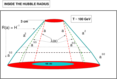
Figure 1: Evolution of the correlation scale for magnetic fields produced inside the Hubble radius. The horizontal thick dashed line marks the end of the radiation-dominated phase and the onset of the matter-dominated phase. The horizontal thin dashed line marks the moment of $e^{+}$–$e^{-}$ annihilation (see also footnoote 2). The full (vertical) lines represent the evolution of the Hubble radius during the different stages of the life of the Universe. The dashed (vertical) lines illustrate the evolution of the correlation scale of the magnetic fields. In the absence of inverse cascade the evolution of the correlation scale is given by the (inner) vertical dashed lines. If inverse cascade takes place the evolution of the correlation scale is faster than the first power of the scale factor (for instance $a^{5/3}$) but always slower than the Hubble radius.

In Fig. 1 we report a schematic illustration of the evolution of the Hubble radius $R_{H}$ and of the correlation scale of the magnetic field as a function of the scale factor. In Fig. 1 the horizontal dashed line simply marks the end of the radiation-dominated phase and the onset of the matter dominated phase: while above the dashed line the Hubble radius evolves as $a^{2}$ (where $a$ is the scale factor), below the dashed line the Hubble radius evolves as $a^{3/2}$.

We consider, for simplicity, a magnetic field whose typical correlation scale is as large as the Hubble radius at the electro-weak epoch when the temperature of the plasma was of the order of $100\,\,{\rm GeV}$. This is roughly the regime contemplated by the considerations presented around Eq. (40). If the correlation scale evolves as the scale factor, the Hubble radius at the electroweak epoch (roughly $3$ cm) projects today over a scale of the order of the astronomical unit. If inverse cascades are invoked, the correlation scale may grow, depending on the specific features of the cascade, up to $100$ A.U. or even up to $100$ pc. In both cases the final scale is too small if compared with the typical scale of the gravitational collapse of the proto-galaxy. In Fig. 1 a particular model for the evolution of the correlation scale $\lambda(a)$ has been reported .

2.6 Inflationary magnetogenesis

If magnetogenesis takes place inside the Hubble radius the main problem is therefore the correlation scale of the obtained seed field. The cure for this problem is to look for a mechanism producing magnetic fields that are coherent over large-scales (i.e. Mpc and, in principle, even larger). This possibility may arise in the context of inflationary models. Inflationary models may be conventional (i.e. based on a quasi-de Sitter stage of expansion) or unconventional (i.e. not based on a quasi-de Sitter stage of expansion). Unconventional inflationary models are, for instance, pre-big bang models that will be discussed in more depth in Section 3.

The rationale for the previous statement is that, in inflationary models, the zero-point (vacuum) fluctuations of fields of various spin are amplified. Typically fluctuations of spin 0 and spin 2 fields. The spin 1 fields enjoy however of a property, called Weyl invariance, that seems to forbid the amplification of these fields. While Weyl invariance and its possible breaking will be the specific subject of the following subsection, it is useful for the moment to look at the kinematical properties by assuming that, indeed, also spin 1 field can be amplified.

Since during inflation the Hubble radius is roughly constant (see Fig. 2), the correlation scale evolves much faster than the Hubble radius itself and, therefore, large scale magnetic domains can naturally be obtained. Notice that, in Fig. 2 the (vertical) dashed lines illustrate the evolution of the Hubble radius (that is roughly constant during inflation) while the full line denotes the evolution of the correlation scale. Furthermore, the horizontal (dashed) lines mark, from top to bottom, the end of the inflationary phase and the onset of the matter-dominated phase. This phenomenon can be understood as the gauge counterpart of the super-adiabatic amplification of the scalar and tensor modes of the geometry. The main problem, in such a framework, is to get large amplitudes for scale of the order of the ${\rm Mpc}$ at the onset of gravitational collapse. Models where the gauge couplings are effectively dynamical (breaking, consequently, the Weyl invariance of the evolution equations of Abelian gauge modes) may provide rather intense magnetic fields.

The two extreme possibilities mentioned above may be sometimes combined. For instance, it can happen that magnetic fields are produced by super-adiabatic amplification of vacuum fluctuations during an inflationary stage of expansion. After exiting the horizon, the gauge modes will reenter at different moments all along the radiation and matter dominated epochs. The spectrum of the primordial gauge fields after reentry will not only be determined by the amplification mechanism but also on the plasma effects. As soon as the magnetic inhomogeneities reenter, some other physical process, taking place inside the Hubble radius, may be triggered by the presence of large scale magnetic fields. An example, in this context, is the production of topologically non-trivial configurations of the hypercharge field (hypermagnetic knots) from a stochastic background of hypercharge fields with vanishing helicity hmk1 ; hmk2 ; hmk3 (see also anomaly ; bdv1 ; bdv2 ; bamba0 ; angel ).

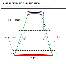
Figure 2: Evolution of the correlation scale if magnetic fields would be produced by superadiabatic amplification during a conventional inflationary phase. The dashed vertical lines denote, in the present figure, the evolution of the Hubble radius while the full line denotes the evolution of the correlation scale (typically selected to smaller than the Hubble radius during inflation).

2.7 Breaking of conformal invariance

Consider the action for an Abelian gauge field in four-dimensional curved space-time

$$S_{\rm em}=-\frac{1}{4}\int d^{4}x\sqrt{-G}F_{\mu\nu}F^{\mu\nu}.$$ (48)

Suppose, also, that the geometry is characterized by a conformally flat line element of Friedmann-Robertson-Walker type as the one introduced in Eq. (46). The equations of motion derived from Eq. (48) can be written as

$$\partial_{\mu}\biggl{(}\sqrt{-G}F^{\mu\nu}\biggr{)}=0.$$ (49)

Using Eq. (46) and recalling that $\sqrt{-G}=a^{4}(\tau)$, we will have

$$\sqrt{-G}F^{\mu\nu}=a^{4}(\tau)\frac{\eta^{\mu\alpha}}{a^{2}(\tau)}\frac{\eta^{\nu\beta}}{a^{2}(\tau)}F_{\alpha\beta}=F^{\mu\nu}$$ (50)

where the second equality follows from the explicit form of the metric. Equation (50) shows that the evolution equations of Abelian gauge fields are the same in flat space-time and in a conformally flat FRW space-time. This property is correctly called Weyl invariance or, more ambiguously, conformal invariance. Weyl invariance is realized also in the case of chiral (massless) fermions always in the case of conformally flat space-times.

One of the reasons of the success of inflationary models in making predictions is deeply related with the lack of conformal invariance of the evolution equations of the fluctuations of the geometry. In particular it can be shown that the tensor modes of the geometry (spin 2) as well as the scalar modes (spin 0) obey evolution equations that are not conformally invariant. This means that these modes of the geometry can be amplified and eventually affect, for instance, the temperature autocorrelations as well as the polarization power spectra in the microwave sky.

To amplify large-scale magnetic fields, therefore, we would like to break conformal invariance. Before considering this possibility, let us discuss an even more conservative approach consisting in studying the evolution of Abelian gauge fields coupled to another field whose evolution is not Weyl invariant. An elegant way to achieve this goal is to couple the action of the hypercharge field to the one of a complex scalar field (the Higgs field). The Abelian-Higgs model, therefore, leads to the following action

$$S=\int d^{4}x\sqrt{-G}\biggl{[}G^{\mu\nu}({\mathcal{D}}_{\mu})^{\ast}\phi{\mathcal{D}}_{\nu}\phi-m^{2}\phi^{\ast}\phi-\frac{1}{4}{\mathcal{F}}_{\mu\nu}{\mathcal{F}}^{\mu\nu}\biggr{]},$$ (51)

where ${\mathcal{D}}_{\mu}=\partial_{\mu}-ie{\mathcal{A}}_{\mu}$ and ${\mathcal{F}}_{\mu\nu}=\partial_{[\mu}{\mathcal{A}}_{\nu]}$. Using Eq. (46) into Eq. (51) and assuming that the complex scalar field (as well as the gauge fields) are not a source of the background geometry, the canonical action for the normal modes of the system can be written as

$$S=\int d^{3}xd\tau\biggl{[}\eta^{\mu\nu}(D_{\mu}\Phi)^{\ast}D_{\nu}\Phi+\biggl{(}\frac{a^{\prime\prime}}{a}-m^{2}a^{2}\biggr{)}\Phi^{\ast}\Phi-\frac{1}{4}F_{\alpha\beta}F^{\alpha\beta}\biggr{]},$$ (52)

where $\Phi=a\phi$; $D_{\mu}=\partial_{\mu}-ieA_{\mu}$ and $F_{\mu\nu}=\partial_{[\mu}A_{\nu]}$. From Eq. (52) it is clear that also when the Higgs field is massless the coupling to the geometry breaks explicitly Weyl invariance. Therefore, current density and charge density fluctuations will be induced. Then, by employing a Vlasov-Landau description similar the resulting magnetic field will be of the order of $B_{\rm dec}\sim 10^{-40}T_{\rm dec}^{2}$ gioshap which is, by far, too small to seed any observable field even assuming, optimistically, perfect flux freezing and maximal efficiency for the dynamo action. The results of gioshap disproved earlier claims (see mgs2 for a critical review) neglecting the rôle of the conductivity in the evolution of large-scale magnetic fields after inflation.

The first attempts to analyze the Abelian-Higgs model in De Sitter space have been made by Turner and Widrow turnerwidrow who just listed such a possibility as an open question. These two authors also analyzed different scenarios where conformal invariance for spin 1 fields could be broken in 4 space-time dimensions. Their first suggestion was that conformal invariance may be broken, at an effective level, through the coupling of photons to the geometry drummond . Typically, the breaking of conformal invariance occurs through products of gauge-field strengths and curvature tensors, i.e.

$$\frac{1}{m^{2}}F_{\mu\nu}F_{\alpha\beta}R^{\mu\nu\alpha\beta},~{}~{}~{}~{}~{}~{}~{}\frac{1}{m^{2}}R_{\mu\nu}F^{\mu\beta}F^{\nu\alpha}g_{\alpha\beta},~{}~{}~{}~{}~{}~{}\frac{1}{m^{2}}F_{\alpha\beta}F^{\alpha\beta}R$$ (53)

where $m$ is the appropriate mass scale; $R_{\mu\nu\alpha\beta}$ and $R_{\mu\nu}$ are the Riemann and Ricci tensors and $R$ is the Ricci scalar. If the evolution of gauge fields is studied during phase of de Sitter (or quasi-de Sittter) expansion, then the amplification of the vacuum fluctuations induced by the couplings listed in Eq. (53) is minute. The price in order to get large amplification should be, according to turnerwidrow , an explicit breaking of gauge-invariance by direct coupling of the vector potential to the Ricci tensor or to the Ricci scalar, i.e.

$$RA_{\mu}A^{\mu},~{}~{}~{}~{}~{}~{}~{}~{}~{}R_{\mu\nu}A^{\mu}A^{\nu}.$$ (54)

In turnerwidrow two other different models were proposed (but not scrutinized in detail) namely scalar electrodynamics and the axionic coupling to the Abelian field strength.

Dolgov dolgov considered the possible breaking of conformal invariance due to the trace anomaly. The idea is that the conformal invariance of gauge fields is broken by the triangle diagram where two photons in the external lines couple to the graviton through a loop of fermions. The local contribution to the effective action leads to the vertex $(\sqrt{-g})^{1+\epsilon}F_{\alpha\beta}F^{\alpha\beta}$ where $\epsilon$ is a numerical coefficient depending upon the number of scalars and fermions present in the theory. The evolution equation for the gauge fields, can be written, in Fourier space, as

$${\cal A}_{k}^{\prime\prime}+\frac{\epsilon}{8}{\cal H}{\cal A}_{k}^{\prime}+k^{2}{\cal A}_{k}=0,$$ (55)

and it can be shown that only if $\epsilon>0$ the gauge fields are amplified. Furthermore, only is $\epsilon\sim 8$ substantial amplification of gauge fields is possible.

In a series of papers carroll1 ; carroll2 ; carroll3 the possible effect of the axionic coupling to the amplification of gauge fields has been investigated. The idea is here that conformal invariance is broken through the explicit coupling of a pseudo-scalar field to the gauge field (see Section 5), i.e.

$$\sqrt{-g}c_{\psi\gamma}\alpha_{\rm em}\frac{\psi}{8\pi M}F_{\alpha\beta}\tilde{F}^{\alpha\beta},$$ (56)

where $\tilde{F}^{\alpha\beta}$ is the dual field strength and where $c_{\psi\gamma}$ is a numerical factor of order one. Consider now the case of a standard pseudoscalar potential, for instance $m^{2}\psi^{2}$, evolving in a de Sitter (or quasi-de Sitter space-time). It can be shown, rather generically, that the vertex given in Eq. (56) leads to negligible amplification at large length-scales. The coupled system of evolution equations to be solved in order to get the amplified field is

$$\vec{B}^{\prime\prime}-\nabla^{2}\vec{B}-\frac{\alpha_{\rm em}}{2\pi M}\psi^{\prime}\vec{\nabla}\times\vec{B}=0,$$ (57)

$$\psi^{\prime\prime}+2{\cal H}\psi^{\prime}+m^{2}a^{2}\psi=0,$$ (58)

where $\vec{B}=a^{2}\vec{B}$. From Eq. (57), there is a maximally amplified physical frequency

$$\omega_{\rm max}\simeq\frac{\alpha_{{\rm em}}}{2\pi M}\dot{\psi}_{\rm max}\simeq\frac{\alpha_{{\rm em}}}{2\pi}m$$ (59)

where the second equality follows from $\psi\sim a^{-3/2}M\cos{mt}$ (i.e. $\dot{\psi}_{\rm max}\sim mM$). The amplification for $\omega\sim\omega_{\rm max}$ is of the order of $\exp{[m\alpha_{\rm em}/(2\pi H)]}$ where $H$ is the Hubble parameter during the de Sitter phase of expansion. From the above expressions one can argue that the modes which are substantially amplifed are the ones for which $\omega_{\rm max}\gg H$. The modes interesting for the large-scale magnetic fields are the ones which are in the opposite range, i.e. $\omega_{\rm max}\ll H$. Clearly, by lowering the curvature scale of the problem the produced seeds may be larger and the conclusions much less pessimistic carroll3 .

Another interesting idea pointed out by Ratra ratra is that the electromagnetic field may be directly coupled to the inflaton field. In this case the coupling is specified through a parameter $\alpha$, i.e. $e^{\alpha\varphi}F_{\alpha\beta}F^{\alpha\beta}$ where $\varphi$ is the inflaton field in Planck units. In order to get sizable large-scale magnetic fields the effective gauge coupling must be larger than one during inflation (recall that $\varphi$ is large, in Planck units, at the onset of inflation).

In variation it has been suggested that the evolution of the Abelian gauge coupling during inflation induce the growth of the two-point function of magnetic inhomogeneities. This model is different from the one previously discussed ratra . Here the dynamics of the gauge coupling is not related to the dynamics of the inflaton which is not coupled to the Abelian field strength. In particular, $r_{B}({\rm Mpc})$ can be as large as $10^{-12}$. In variation the MHD equations have been generalized to the case of evolving gauge coupling. Recently a scenario similar to variation has been discussed in bamba .

In the perspective of generating large scale magnetic fields Gasperini gravphot suggested to consider the possible mixing between the photon and the graviphoton field appearing in supergravity theories (see also, in a related context okun ). The graviphoton is the massive vector component of the gravitational supermultiplet and its interaction with the photon is specified by an interaction term of the type $\lambda F_{\mu\nu}G^{\mu\nu}$ where $G_{\mu\nu}$ is the filed strength of the massive vector. Large-scale magnetic fields with $r_{B}({\rm Mpc})\geq 10^{-34}$ can be obtained if $\lambda\sim{\cal O}(1)$ and for a mass of the vector $m\sim 10^{2}{\rm TeV}$.

Bertolami and Mota bertolami argue that if Lorentz invariance is spontaneously broken, then photons acquire naturally a coupling to the geometry which is not gauge-invariant and which is similar to the coupling considered in turnerwidrow .

3 Why string cosmology?

The moment has come to review my personal interaction with Gabriele Veneziano on the study of large-scale magnetic fields. While we had other 15 joined papers with Gabriele (together with different combinations of authors) two of them GAB1 ; GAB2 (both in collaboration with Maurizio Gasperini) are directly related to large-scale magnetic fields. Both papers reported in Refs. GAB1 ; GAB2 appeared in 1995 while I was completing my Phd at the theory division of CERN.

My scientific exchange with Gabriele Veneziano started at least four years earlier and the first person mentioning Gabriele to me was Sergio Fubini. At that time Sergio was professor of Theoretical Physics at the University of Turin and I had the great opportunity of discussing physics with him at least twice a month. Sergio was rather intrigued by the possibility of getting precise measurements on macroscopic quantum phenomena like superfluidity, superconductivity, quantization of the resistivity in the (quantum) Hall effect. I started working, under the supervision of Maurizio Gasperini, on the spectral properties of relic gravitons and we bumped into the concept of squeezed state gg , a generalization of the concept of coherent state (see, for instance, stoler ; luciano ; yuen ). Sergio got very interested and, I think, he was independently thinking about possible applications of squeezed states to superconductivity, a topic that became later on the subject of a paper mol . Sergio even suggested a review by Rodney Loudon loudon , an author that I knew already beacuse of his inspiring book on quantum optics loudon2 . Ref. loudon together with a physics report of B. L. Schumaker schumi was very useful for my understanding of the subject. Nowadays a very complete and thorough presentation of the intriguing problems arising in quantum optics can be found in the book of Leonard Mandel and Emil Wolf mandel .

It is amusing to notice the following parallelism between quantum optics and the quantum treatment of gravitational fluctuations. While quantum optics deals with the coherence properties of systems of many photons, we deal, in cosmology, with the coherence properties of many gravitons (or phonons) excited during the time-evolution of the background fields. The background fields act, effectively, as a ”pump field”. This terminology, now generally accepted, is exactly borrowed by quantum optics where the pump field is a laser. In the sixties and seventies the main problem of optics can be summarized by the following question: why is classical optics so precise? Put it into different words, it is known that the interference of the amplitudes of the radiation field (the so-called Young interferometry) can be successfully treated at a classical level. Quantum effects, in optics, arise not from the first -order interference effects (Young interferometry) but from the second-order interference effects, i.e. the so-called Hanbury-Brown-Twiss interferometry mandel where the quantum nature of the radiation field is manifest since it leads, in the jargon introduced by Mandel mandel to light which is either bunched or anti-bunched. A similar problem also arises in the treatment of cosmological perturbations when we ask the question of the classical limit of a quantum mechanically generated fluctuation (for instance relic gravitons).

The interaction with Sergio led, few years later, to a talk that I presented at the physics department of the University of Torino. The title was Correlation properties of many photons systems. I mentioned my interaction with Sergio Fubini since it was Sergio who suggested that, eventually, I should talk to Gabriele about squeezed states.

During the first few months of 1991, Gabriele submitted a seminal paper on the cosmological implications of the low-energy string effective action PBB1 . This paper, together with another one written in collaboration with Maurizio Gasperini PBB2 represents the first formulation of pre-big bang models. A relatively recent introduction to pre-big bang models can be found in Ref. PBB3 .

In GAB1 ; GAB2 it was argued that the string cosmological scenario provided by pre-big bang models PBB1 ; PBB2 would be ideal for the generation of large-scale magnetic fields. The rationale for this statement relies on two different observations:

• in the low-energy string effective action gauge fields are coupled to the dilaton whose expectation value, at the string energy scale, gives the unified value of the gauge and gravitational coupling;

• from the mathematical analysis of the problem it is clear that to achieve a sizable amplification of large-scale magnetic fields it is necessary to have a pretty long phase where the gauge coupling is sharply growing in time GAB1 .

Let us therefore elaborate on the two mentioned points. In the string frame the low-energy string effective action can be schematically written as LEST1 ; LEST2 ; LEST3

$$S_{\rm eff}=-\int d^{4}x\sqrt{-G}\biggl{[}\frac{e^{-\varphi}}{2\lambda_{\rm s}^{2}}\biggl{(}R+G^{\alpha\beta}\partial_{\alpha}\varphi\partial_{\beta}\varphi-\frac{1}{12}H_{\mu\nu\alpha}H^{\mu\nu\alpha}\biggr{)}$$

$$+\frac{e^{-\varphi}}{4}F_{\alpha\beta}F^{\alpha\beta}+e^{-\varphi}\overline{\psi}\biggl{(}\frac{i}{2}\gamma^{\mathrm{a}}D_{\mathrm{a}}\psi+{\mathrm{h}.c.}\biggr{)}+{\mathcal{R}}^{2}+\,.......\biggr{]}+{\mathcal{O}}(g^{2})+\,....$$ (60)

In Eq. (60) the ellipses stand, respectively, for an expansion in powers of $(\lambda_{\rm s}/L)^{2}$ and for an expansion in powers of the gauge coupling constant $g^{2}=e^{\varphi}$. This action is written in the so-called string frame metric where the dilaton field $\varphi$ is coupled to the Einstein-Hilbert term.

Concerning the action (60) few general comments are in order

• the relation between the Planck and string scales depends on time and, in particular, $\ell_{\mathrm{P}}^{2}=e^{\varphi}\lambda_{\mathrm{s}}^{2}$; the present ratio between the Planck and string scales gives the value, i.e. $g(\tau_{0})=e^{\varphi_{0}/2}=\ell_{P}(\tau_{0})/\lambda_{\rm s}$;

• in four space-time dimensions the antisymmetric tensor field $H^{\mu\nu\alpha}$ can be written in terms of a pseudo-scalar field, i.e.

  $$H^{\mu\nu\alpha}=e^{\varphi}\frac{\epsilon^{\mu\nu\alpha\rho}}{\sqrt{-G}}\partial_{\rho}\sigma;$$ (61)

In critical superstring theory the dilaton field must have a potential that vanishes in the weak coupling limit (i.e. $\varphi\to-\infty$). Moreover, from the direct tests of Newton law at short distances it should also happen that the mass of the dilaton is such that $m_{\varphi}>10^{-4}$. This requirement may be relaxed by envisaging non-perturbative mechanisms where the dilaton is effectively decoupled from the matter fields and where a massless dilaton leads to observable violations of the equivalence principle.

From the structure of the action (60), Abelian gauge fields are amplified if the gauge coupling is dynamical. Consider, in fact, the equations of motion for the hypercharge field strength

$$\partial_{\mu}\biggl{(}e^{-\varphi}\sqrt{-G}F^{\mu\nu}\biggr{)}=0,$$ (62)

where $F_{\mu\nu}=\partial_{[\mu}A_{\nu]}$. In the Coulomb gauge where $A_{0}=0$ and $\vec{\nabla}\cdot\vec{A}=0$ the equation for the rescaled vector potential ${\mathcal{A}}_{\mu}=e^{\varphi/2}A_{\mu}$ becomes, for each independent polarization and in Fourier space,

$${\mathcal{A}}_{k}^{\prime\prime}+\biggl{[}k^{2}-g\biggl{(}\frac{1}{g}\biggr{)}^{\prime\prime}\biggr{]}{\mathcal{A}}_{k}=0,$$ (63)

where, as usual, the prime denotes a derivation with respect to the conformal time coordinate. In Eq. (63) $k$ denotes the comoving wave-number From the structure of Eq. (63) there exist two different regimes. For $k^{2}\gg|g(g^{-1})^{\prime\prime}|$ the solution off Eq. (63) is oscillatory. In the opposite limit, i.e. $k^{2}\ll|g(g^{-1})^{\prime\prime}|$ the general solution can be written as

$${\mathcal{A}}_{k}(\tau)=\frac{C_{1}(k)}{g(\tau)}+\frac{C_{2}(k)}{g(\tau)}\int^{\tau}g^{2}(\tau^{\prime})d\tau^{\prime},$$ (64)

where $C_{1}(k)$ and $C_{2}(k)$ are two arbitrary constants. These two constants can be fixed by imposing quantum mechanical initial conditions for $\tau\to-\infty$. Thus, depending on the evolution of $g(\tau)$ the Fourier amplitude ${\mathcal{A}}_{k}$ can be amplified.

It can be shown GAB1 ; GAB2 that the the amplified magnetic energy density depends on the ratio between the value of the gauge coupling at the reentry and at the exit of the typical scale of the gravitational collapse, i.e.

$$r(k)=\frac{1}{\rho_{\gamma}}\frac{d\rho_{\mathrm{B}}}{d\ln{k}}\simeq\frac{k^{4}}{a^{4}\rho_{\gamma}}\biggl{(}\frac{g_{\mathrm{r}e}}{g_{\mathrm{e}x}}\biggr{)}^{2}.$$ (65)

The parameter $r(k)$ measures the relative weight of the magnetic energy density in units of the radiation background. To turn on the galactic dynamo in its simplest realization one should require that $r(k_{\mathrm{G}})\geq 10^{-34}$ for a typical comoving wave-number corresponding to the typical scale of the gravitational collapse of the protogalaxy. As explained before, this requirement seems to be too optimistic in the light of the most recent understanding of the dynamo theory. The limit $r(k_{\rm G})\geq 10^{-24}$ seems more reasonable.

The fact that the gauge coupling must be sharply growing in order to produce large-scale magnetic fields fits extremely well with the pre-big bang dynamics where, indeed, the gauge coupling is expected to grow. The second requirement to obtain a phenomenologically viable mechanism for the amplification of large-scale gauge fields turned out to be the existence of a pretty long stringy phase.

The ”stringy” phase is simply the epoch where quadratic curvature corrections start being important and lead to an effective dynamics where the dilaton field is linearly growing in the cosmic time coordinate (see PBB3 and references therein). Towards the end of the stringy phase the dilaton freezes to its (constant) value and the Universe gets dominated by radiation. One possibility for achieving the transition to radiation is represented by the back-reaction effects of the produced particles heating . In particular, the short wavelength modes play, in this context a crucial rôle. It is interesting that while the magnetic energy spectrum produced during the stringy phase is quasi-flat and the value of $r(k_{\mathrm{G}})$ can be as large as $10^{-8}$ implying a protogalactic magnetic field of the order of $10^{-10}$ G. Under these conditions the dynamo mechanism would even be superfluous since the compressional amplification alone can amplify the seed field to its observed value.

The results reported above may be “tested” in a framework where the pre-big bang dynamics is solvable. Consider, in particular, the situation where the evolution of the dilaton field as well as the one of the geometry is treated in the presence of a non-local dilaton potential G1 ; G2 ; meis0 ; meis1 ; gmv .

In the Einstein frame description, the asymptotics of the (four-dimensional) pre-big bang dynamics can be written as heating

$$a(\tau)\simeq a_{-}\sqrt{-\frac{\tau}{2\tau_{0}}},~{}~{}~{}~{}~{}~{}~{}~{}a_{-}=e^{-\varphi_{0}/2}\sqrt{\frac{2(\sqrt{3}+1)}{\sqrt{3}}},$$

$$\varphi_{-}=\varphi_{0}-\ln{2}-\sqrt{3}\ln{\biggl{(}\frac{\sqrt{3}+1}{\sqrt{3}}\biggr{)}}-\sqrt{3}\ln{\biggl{(}-\frac{\tau}{2\tau_{0}}\biggr{)}},$$

$${\cal H}_{-}=\frac{1}{2\tau},~{}~{}~{}~{}~{}~{}~{}~{}~{}~{}~{}~{}~{}~{}~{}\varphi_{-}^{\prime}=-\frac{\sqrt{3}}{\tau},$$ (66)

for $\tau\to-\infty$, and

$$a(\tau)\simeq a_{+}\sqrt{\frac{\tau}{2\tau_{0}}},~{}~{}~{}~{}~{}~{}~{}~{}~{}~{}~{}~{}a_{+}=e^{\varphi_{0}/2}\sqrt{\frac{2(\sqrt{3}-1)}{\sqrt{3}}}$$

$$\varphi_{+}=\varphi_{0}-\ln{2}-\sqrt{3}\ln{\biggl{(}\frac{\sqrt{3}-1}{\sqrt{3}}\biggr{)}}+\sqrt{3}\ln{\biggl{(}\frac{\tau}{2\eta_{0}}\biggr{)}},$$

$${\cal H}_{+}=\frac{1}{2\tau},~{}~{}~{}~{}~{}~{}~{}~{}~{}~{}~{}~{}~{}~{}~{}\varphi_{+}^{\prime}=\frac{\sqrt{3}}{\tau},$$ (67)

for $\tau\to+\infty$. In Eqs. (66) and (67), ${\mathcal{H}}=a^{\prime}/a$ and, as usual, the prime denotes a derivation with respect to $\tau$.The branch of the solution denoted by minus describes, in the Einstein frame, an accelerated contraction, since the first derivative of the scale factor is negative while the second is positive. The branch of the solution denoted with plus describes, in the Einstein frame, a decelerated expansion, since the first derivative of the scale factor is positive while the derivative is negative. In both branches the dilaton grows and its derivative is always positive-definite (i.e. $\varphi^{\prime}_{\pm}>0$ ) as required by the present approach to bouncing solutions. The numerical solution corresponding to the asymptotics given in Eqs. (66) and (67) is reported in Fig. 3

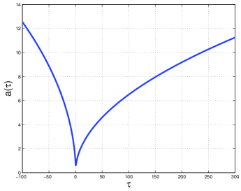
Figure 3: The evolution of the scale factor in conformal time for a bouncing model regularized via non-local dilaton potential in the Einstein frame.

In the Schrödinger description the vacuum state evolves, unitarily, to a multimode squeezed state, in full analogy with what happens in the case of relic gravitons squeezed1 ; squeezed2 ; squeezed3 . In the following the same process will be discussed within the Heisenberg representation. The two physical polarizations of the photon can then be quantized according to the standard rules of quantization in the radiation gauge in curved space-times:

$$\hat{\cal A}_{i}(\vec{x},\tau)=\sum_{\alpha}\int\frac{d^{3}k}{(2\pi)^{3/2}}\biggl{[}\hat{a}_{k,\alpha}e^{\alpha}_{i}{\cal A}_{k}(\tau)e^{-i\vec{k}\cdot\vec{x}}+\hat{a}_{k,\alpha}^{\dagger}e_{i}^{\alpha}{\cal A}_{k}(\tau)^{\star}e^{i\vec{k}\cdot\vec{x}}\biggr{]},$$ (68)

and

$$\hat{\pi}_{i}(\vec{x},\tau)=\sum_{\alpha}\int\frac{d^{3}k}{(2\pi)^{3/2}}\biggl{[}\hat{a}_{k,\alpha}e^{\alpha}_{i}\Pi_{k}(\tau)e^{-i\vec{k}\cdot\vec{x}}+\hat{a}_{k,\alpha}^{\dagger}e_{i}^{\alpha}\Pi_{k}(\tau)^{\star}e^{i\vec{k}\cdot\vec{x}}\biggr{]},$$ (69)

where $e_{i}^{\alpha}(k)$ describe the polarizations of the photon and

$$\Pi_{k}(\tau)={\cal A}_{k}^{\prime}(\tau),~{}~{}~{}~{}~{}~{}~{}~{}~{}[\hat{a}_{k,\alpha},\hat{a}_{p,\beta}^{\dagger}]=\delta_{\alpha\beta}\delta^{(3)}(\vec{k}-\vec{p}).$$ (70)

The evolution equation for the mode functions will then be, in Fourier space,

$${\cal A}_{k}^{\prime\prime}+\biggl{[}k^{2}-g(g^{-1})^{\prime\prime}\biggr{]}{\cal A}_{k}=0,$$ (71)

i.e. exactly the same equation obtained in (63). The pump field can also be expressed as:

$$g(g^{-1})^{\prime\prime}=\biggl{(}\frac{{\varphi^{\prime}}^{2}}{4}-\frac{\varphi^{\prime\prime}}{2}\biggr{)}.$$ (72)

The maximally amplified modes are then the ones for which

$$k_{\rm max}^{2}\simeq|g(g^{-1})^{\prime\prime}|.$$ (73)

The Fourier modes appearing in Eq. (71) have to be normalized while they are inside the horizon for large and negative $\tau$. In this limit the initial conditions provided by quantum mechanics are

$${\cal A}_{k}(\tau)=\frac{1}{\sqrt{2k}}e^{-ik\tau},\qquad\Pi_{k}(\tau)=-i\sqrt{\frac{k}{2}}e^{-ik\tau}.$$ (74)

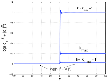
Figure 4: The evolution of the mixing coefficients for $k\simeq k_{\mathrm{kmax}}$ in units of $\tau_{0}$.

In the limit $\tau\to+\infty$ the positive and negative frequency modes will be mixed, so that the solution will be represented in the plane wave orthonormal basis as

$${\cal A}_{k}(\tau) = \frac{1}{\sqrt{2k}}\biggl{[}c_{+}(k)e^{-ik\tau}+c_{-}(k)e^{ik\tau}\biggr{]},$$

$${\cal A}_{k}^{\prime}(\tau) = -i\sqrt{\frac{k}{2}}\biggl{[}c_{+}(k)e^{-ik\tau}-c_{-}(k)e^{ik\tau}\biggr{]}.$$ (75)

where $c_{\pm}(k)$ are the (constant) mixing coefficients. The following two relations fully determine the square modulus of each of the two mixing coefficients in terms of the complex wave-functions obeying Eq. (71):

$$|c_{+}(k)|^{2}-|c_{-}(k)|^{2}=i({\cal A}_{k}^{\star}\Pi_{k}-{\cal A}_{k}\Pi_{k}^{\star}),$$ (76)

$$|c_{+}(k)|^{2}+|c_{-}(k)|^{2}=\frac{1}{k^{2}}\biggl{(}|\Pi_{k}|^{2}+k^{2}|{\cal A}_{k}|^{2}\biggr{)}.$$ (77)

After having numerically computed the time evolution of the properly normalized mode functions, Eqs. (76) and (77) can be used to infer the value of the relevant mixing coefficient (i.e. $c_{-}(k)$). Equation (76) is, in fact, the Wronskian of the solutions. If the second-order differential equation is written in the form (71), the Wronskian is always conserved throughout the time evolution of the system. Since, from Eq. (74), the Wronskian is equal to $1$ initially, it will be equal to $1$ all along the time evolution. Thus, from Eq. (76) $|c_{+}(k)|^{2}=|c_{-}(k)|^{2}+1$. The fact that the Wronskian must always be equal to $1$ is the measure of the precision of the algorithm.

In Figs. 4 and 5 the numerical calculation of the spectrum is illustrated for different values of $k$. In Fig. 5 the mixing coefficients are reported for modes $k\ll k_{\rm max}$. In Fig. 4 the mixing coefficients are reported for modes around $k_{\rm max}$. Clearly, from Fig. 5 a smaller $k$ leads to a larger mixing coefficient which means that the spectrum is rather blue. Furthermore by comparing the amplification of different modes it is easy to infer that the scaling law is $|c_{+}(k)|^{2}+|c_{-}(k)|^{2}\propto(k/k_{\rm max})^{-n_{g}}$ , with $n_{g}\sim 3.46$, which is in excellent agreement with the analytical determination of the mixing coefficients leading to $n_{g}=2\sqrt{3}\sim 3.46$[see below, Eq. (88)].

The second piece information that can be drawn from Fig. 4 concerns $k_{\rm max}$, whose specific value

$$k_{\rm max}\simeq\frac{\sqrt{5}-0.5}{\tau_{0}}.$$ (78)

can be determined numerically for different values of $\tau_{0}$.

For the value of $k_{\rm max}$ reported in Eq. (78), the obtained mixing coefficient is $1$, i.e. $|c_{-}(k_{\rm max})|\simeq 1$. According to Fig. 4 as we move from $k_{\rm max}$ to larger $k$, $(|c_{+}(k)|^{2}+|c_{-}(k)|^{2})\simeq(|c_{+}(k)|^{2}-|c_{-}(k)|^{2})$ implying that $|c_{-}(k)|\sim 0$. Moreover, from the left plot of Fig. 5 it can be appreciated that

$$|c_{-}(k_{\rm max})|^{2}=1,~{}~{}~{}~{}~{}\log{(|c_{+}(k_{\rm max})|^{2}+|c_{-}(k_{\rm max})|^{2})}=\log{3}\simeq 0.477.$$ (79)

Thus the absolute normalization and slope of the relevant mixing coefficient can be numerically determined to be

$$|c_{-}(k)|^{2}=\biggl{(}\frac{k}{k_{\rm max}}\biggr{)}^{-2\sqrt{3}}.$$ (80)

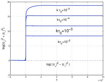
Figure 5: The numerical estimate of the mixing coefficients in the case $k\tau_{0}\ll 1$.

It can be concluded that Eq. (80) is rather accurate as far as both the slope and the absolute normalization are concerned. The numerical estimates presented so far can be also corroborated by the usual analytical treatment based on the matching of the solutions for the mode functions before and after the bounce. The evolution of the modes described by Eq. (71) can be approximately determined from the exact asymptotic solutions given in Eqs. (66) and (67), and implying that $\varphi^{\prime}_{\pm}\simeq\pm\sqrt{3}/\tau$. Thus the solutions of Eq. (71) can be obtained in the two asymptotic regimes, i.e. for $\tau\leq-\tau_{1}$

$${\cal A}_{k,-}(\tau)=\frac{\sqrt{-\pi\tau}}{2}e^{i\frac{\pi}{2}(\nu+1/2)}H_{\nu}^{(1)}(-k\tau),$$ (81)

and for $\tau\geq\tau_{1}$

$${\cal A}_{k,+}(\eta)=\frac{\sqrt{\pi\tau}}{2}e^{i\frac{\pi}{2}(\mu+1/2)}\biggl{[}c_{-}H_{\mu}^{(1)}(k\tau)+c_{+}e^{-i\pi(\mu+1/2)}H_{\mu}^{(2)}(k\tau)\biggr{]},~{}\tau\geq-\tau_{1},$$ (82)

where $H^{(1,2)}_{\alpha}(z)$ are Hankel functions of first and second kind whose related indices are

$$\nu=\frac{\sqrt{3}-1}{2},~{}~{}~{}~{}~{}~{}~{}~{}~{}~{}~{}\mu=\frac{\sqrt{3}+1}{2}.$$ (83)

The time scale $\tau_{1}$ defines the width of the bounce and, typically, $\tau_{1}\sim\tau_{0}$.

The phases appearing in Eqs. (81) and (82) are carefully chosen so that

$$\lim_{\tau\to-\infty}{\cal A}_{k}=\frac{1}{\sqrt{2k}}e^{-ik\tau}.$$ (84)

Using then the appropriate matching conditions

$${\cal A}_{k,-}(-\tau_{1})={\cal A}_{k,+}(\tau_{1}),$$

$${\cal A}_{k,-}^{\prime}(-\tau_{1})={\cal A}_{k,+}^{\prime}(\tau_{1}),$$ (85)

and defining $x_{1}=k\tau_{1}$, the obtained mixing coefficients are

$$c_{+}(k)=i\frac{\pi}{4}x_{1}e^{i\pi(\nu+\mu+1)/2}\biggl{[}-\frac{\nu+\mu+1}{x_{1}}H_{\mu}^{(1)}(x_{1})H_{\nu}^{(1)}(x_{1})$$

$$+H_{\mu}^{(1)}(x_{1})H_{\nu+1}^{(1)}(x_{1})+H_{\mu+1}^{(1)}(x_{1})H_{\nu}^{(1)}(x_{1})\biggr{]},$$ (86)

$$c_{-}(k)=i\frac{\pi}{4}x_{1}e^{i\pi(\nu-\mu)/2}\biggl{[}-\frac{\nu+\mu+1}{x_{1}}H_{\mu}^{(2)}(x_{1})H_{\nu}^{(1)}(x_{1})$$

$$+H_{\mu}^{(2)}(x_{1})H_{\nu+1}^{(1)}(x_{1})+H_{\mu+1}^{(2)}(x_{1})H_{\nu}^{(1)}(x_{1})\biggr{]},$$ (87)

satisfying the exact Wronskian normalization condition $|c_{+}(k)|^{2}-|c_{-}(k)|^{2}=1$. In the small argument limit, i.e. $k\tau_{1}\sim k\tau_{0}\ll 1$ the leading term in Eq. (87) leads to

$$c_{-}(k)\simeq\frac{i~{}2^{\mu+\nu}}{4\pi}e^{i\pi(\nu-\mu)/2}x_{1}^{-\mu-\nu}(\nu+\mu-1)\Gamma(\mu)\Gamma(\nu)$$ (88)

If we now insert the values given in Eq. (83) it turns out that $c_{-}(k)\simeq 0.41~{}|k\tau_{1}|^{-\sqrt{3}}$. The spectral slope agrees with the numerical estimate, as already stressed. The absolute normalization cannot be determined from Eq. (88), where the small argument limit has already been taken. In order to determine the absolute normalization the specific value of $k_{\rm max}\tau_{1}$ has to be inserted in Eq. (87). The result of this procedure, taking $\tau_{1}\sim\tau_{0}$ is $|c_{-}(k_{\rm max})|^{2}=0.14$, which is roughly a factor of $10$ smaller than the interpolating formula given in Eq. (80).

The observation that a dynamical gauge coupling implies a viable mechanism for the production of large-scale magnetic fields can be interesting in general terms and, more specifically, in the context of the pre-big bang models. In fact, in pre-big bang models, not only the fluctuations of the hypercharge field are amplified. In the minimal case we will have to deal with the fluctuations of the tensor gg ; tens1 and scalar maxmuk modes of the geometry and with the fluctuations of the antisymmetric tensor field sloth ; ax1 .

The amplified tensor modes of the geometry lead to a stochastic background of gravitational waves (GW) with violet spectrum both in the GW amplitude and energy density. In Fig. 6 the GW signal is parametrized in terms of the logarithm of $\Omega_{\rm GW}=\rho_{\rm GW}/\rho_{\rm c}$, i.e. the fraction of critical energy density present (today) in GW. On the horizontal axis of Fig. 6 the logarithm of the present (physical) frequency $\nu$ is reported.

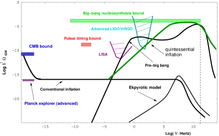
Figure 6: The spectrum of relic gravitons from various cosmological models presented in terms of $h^{2}\Omega_{\rm GW}$ .

In conventional inflationary models, for $\nu\geq 10^{-16}$ Hz, $\Omega_{\rm GW}$, is constant (or slightly decreasing) as a function of the present frequency. In the case of string cosmological models $\Omega_{\rm GW}\propto\nu^{3}\ln{\nu}$, which also implies a steeply increasing power spectrum. This possibility spurred various experimental groups to analyse possible directs limits on the scenario arising from specific instruments such as resonant mass detectors bars and microwave cavities picasso ; cruise . These attempts are justified since the signal of pre-big bang models may be rather strong at high frequencies and, anyway, much stronger than the conventional inflationary prediction

The sensitivity of a pair of VIRGO detectors to string cosmological gravitons has been specifically analysed maxdan with the conclusion that a VIRGO pair, in its upgraded stage, can certainly probe wide regions of the parameter space of these models. If we maximize the overlap between the two detectors maxdan or if we reduce (selectively) the pendulum and pendulum’s internal modes contribution to the thermal noise of the instruments, the visible region (after one year of observation and with ${\rm SNR}=1$) of the parameter space will get even larger. Unfortunately, as in the case of the advanced LIGO detectors, the sensitivity to a flat $\Omega_{\rm GW}$ will be irrelevant for ordinary inflationary models also with the advanced VIRGO detector. It is worth mentioning that growing energy spectra of relic gravitons can also arise in the context of quintessential inflationary models alex2 ; maxquint . In this case $\Omega_{\rm GW}\propto\nu\ln^{2}{\nu}$ (see maxquint for a full discussion).

The spectra of gravitational waves have features that are, in some sense, complementary to the ones of the large-scale magnetic fields. The parameter space leading to a possible signal of relic (pre-big bang) gravitons with wide-band interferometers has only a small overlap with the region of the parameter space leading to sizable large-scale magnetic fields. This conclusion can be evaded if the coupling of the dilaton to the hypercharge field is, in the action, of the type $e^{-\beta\varphi}F_{\mu\nu}F^{\mu\nu}$ nicotri where the parameter $\beta$ has values $1$ and $1/2$, respectively, for heterotic and type I superstrings. In particular, in the case $\beta=1/2$, it is possible to find regions where both large-scale magnetic fields and relic gravitons are copiously produced.

Let us finally discuss the scalar fluctuations of the geometry. The spectrum of the scalar modes is determined by the spectrum of the Kalb-Ramond axion(s). If the axions would be neglected, the spectrum of the curvature fluctuations would be sharply increasing, or as we say in the jargon, the spectrum would be violet in full analogy with the spectrum of the tensor modes of the geometry. This result maxmuk has been recently analyzed in the light of a recent controversy (see G1 ; G2 ) and references therein).

If the Kalb-Ramond axions are consistently included in the calculation, it is found that the large-scale spectrum of curvature perturbations becomes flat ax1 and essentially inherits the spectrum of the Kalb-Ramond axions. If the axions decay (after a phase of coherent oscillations) the curvature perturbations will be adiabatic as in the case of conventional inflationary models but with some important quantitative differences ax1 since, in this case, the CMB normalization is explained in terms of the present value of the string curvature scale and in terms of the primordial slope of the axion spectrum.

4 Primordial or not primordial, this is the question…

While diverse theoretical models for the origin of large-scale magnetism can certainly be questioned on the basis of purely theoretical considerations, direct observations can tell us something more specific concerning the epoch of formation of large-scale magnetic fields. It would be potentially useful to give some elements of response to the following burning question: are really magnetic fields primordial?

The plan of the present section is the following. In Subsect. 4.1 different meanings of the term primordial will be discussed. It will be argued that CMB physics can be used to constrain large-scale magnetic fields possibly present prior to matter-radiation equality. In Subsect. 4.2 the scalar CMB anisotropies will be specifically discussed by deriving the appropriate set of evolution equations accounting for the presence of a fully inhomogeneous magnetic field. In Subsect. 4.3 the evolution of the different species composing the pre-decoupling plasma will be solved, in the tight-coupling approximation and in the presence of a fully inhomogeneous magnetic field. Finally Subsect. 4.4 contains various numerical results and a strategy for parameter extraction.

4.1 Pre-equality magnetic fields

The term primordial seems to have slightly different meanings depending on the perspective of the various communities converging on the study of large-scale magnetic fields. Radio-astronomers have the hope that by scrutinizing the structure of magnetic fields in distant galaxies it would be possible, in the future, to understand if the observed magnetic fields are the consequence of a strong dynamo action or if their existence precedes the formation of galaxies.

If the magnetic field does not flips its sign from one spiral arm to the other, then a strong dynamo action can be suspected beck1 . In the opposite case the magnetic field of galaxies should be primordial i.e. present already at the onset of gravitational collapse. In this context, primordial simply means protogalactic. An excellent review on the evidence of magnetism in nearby galaxies can be found in beck2 .

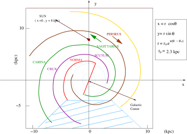
Figure 7: The schematic map of the MW is illustrated. Following vallee the origin of the two-dimensional coordinate system are in the Galactic center. The two large arrows indicate one of the possible (3 or 5) field reversals observed so far.

In Fig. 7 a schematic view of the Milky Way is presented. The magnetic field follows the spiral arm. There have been claims, in the literature, of $3$ to $5$ field reversals. The arrows in Fig. 7 indicate one of the possible field reversals. One reversal is certain beyond any doubt. Another indication that would support the primordial nature of the magnetic field of galaxies would be, for instance, the evidence that not only spirals but also elliptical galaxies are magnetized (even if the magnetic field seems to have correlation scale shorter than in the case of spirals). Since elliptical galaxies have a much less efficient rotation, it seems difficult to postulate a strong dynamo action. We will not pursue here the path of specific astrophysical signatures of a truly pre-galactic magnetic field and e refer the interested reader to beck1 ; beck2 .

As a side remark, it should also be mentioned that magnetic fields may play a rôle in the analysis of rotation curves of spiral galaxies. This aspect has been investigated in great depth by E. Battaner, E. Florido and collaborators also in connection with possible effects of large-scale magnetic fields on structure formation ED1 ; ED2 ; ED3 ; ED4 (see also ED5 and references therein).

The large-scale magnetic fields produced via the parametric amplification of quantum fluctuations discussed earlier in the present lecture may also be defined primordial but, in this case, the term primordial has a much broader signification embracing the whole epoch that precedes the equality between matter and radiation taking place, approximately, at a redshift $z_{\mathrm{e}q}=3230$ for $h^{2}\Omega_{\mathrm{m}0}=0.134$ and $h^{2}\Omega_{\mathrm{r}0}=4.15\times 10^{-5}$. Consequently, large-scale magnetic fields may affect, potentially, CMB anisotropies f1 . Through the years, various studies have been devoted to the effect of large-scale magnetic fields on the vector and tensor CMB anisotropies f3 ; f9 (see also f4 and references therein for some recent review articles).

The implications of fully inhomogeneous magnetic fields on the scalar modes of the geometry remain comparatively less explored. By fully inhomogeneous we mean stochastically distributed fields that do not break the spatial isotropy of the background f4 ; f4a .

CMB anisotropies are customarily described in terms of a set of carefully chosen initial conditions for the evolution of the brightness perturbations of the radiation field. One set of initial conditions corresponds to a purely adiabatic mode. There are, however, more complicated situations where, on top of the adiabatic mode there is also one (or more) non-adiabatic mode(s). A mode, in the present terminology, simply means a consistent solution of the governing equations of the metric and plasma fluctuations, i.e. a consistent solution of the perturbed Einstein equations and of the lower multipoles of the Boltzmann hierarchy.

The simplest set of initial conditions for CMB anisotropies, implies, in a $\Lambda$CDM framework, that a nearly scale-invariant spectrum of adiabatic fluctuations is present after matter-radiation equality (but before decoupling) for typical wavelengths larger than the Hubble radius at the corresponding epoch f5 .

It became relevant, through the years, to relax the assumption of exact adiabaticity and to scrutinize the implications of a more general mixture of adiabatic and non-adiabatic initial conditions (see f60 ; f61 ; f62 and references therein). In what follows it will be argued, along a similar perspective, that large-scale magnetic fields slightly modify the adiabatic paradigm so that their typical strengths may be constrained. To achieve such a goal, the first step is to solve the evolution equations of magnetized cosmological perturbations well before matter-radiation equality. The second step is to follow the solution through equality (and up to decoupling). On a more technical ground, the second step amounts to the calculation of the so-called transfer matrix maxprd06 whose specific form is one of the the subjects of the present analysis.

4.2 Basic Equations

Consider then the system of cosmological perturbations of a flat Friedmann-Robertson-Walker (FRW) Universe, characterized by a conformal time scale factor $a(\tau)$ (see Eq. (46)), and consisting of a mixture of photons, baryons, CDM particles and massless neutrinos. In the following the basic set of equations used in order to describe the magnetized curvature perturbations will be introduced and discussed. The perspective adopted here is closely related to the recent results obtained in Refs. maxprd206 ; maxcqg06 (see also f3a ; f3b for interesting developments).

In the conformally Newtonian gauge f70 ; f71 ; f72 ; f73 ; f74 , the scalar fluctuations of the metric tensor $G_{\mu\nu}=a^{2}(\tau)\eta_{\mu\nu}$ are parametrized in terms of the two longitudinal fluctuations i.e.

$$\delta G_{00}=2a^{2}(\tau)\phi(\tau,\vec{x}),\qquad\delta G_{ij}=2a^{2}(\tau)\psi(\tau,\vec{x})\delta_{ij},$$ (89)

where $\delta_{ij}$ is the Kroeneker $\delta$. While the spatial curvature will be assumed to vanish, it is straightforward to extend the present considerations to the case when the spatial curvature is not negligible.

In spite of the fact that the present discussion will be conducted within the conformally Newtonian gauge, it can be shown that gauge-invariant descriptions of the problem are possible maxcqg06 . Moreover, specific non-adiabatic modes (like the ones related to the neutrino system) may be more usefully described in different gauges (like the synchronous gauge). The rationale for the last statement is that the neutrino isocurvature modes may be singular in the conformally Newtonian gauge. These issues will not be addressed here but have been discussed in the existing literature (see, for instance, f73 ; f74 and references therein). Furthermore, for the benefit of the interested reader it is appropriate to mention that the relevant theoretical tools used in the present and in the following paragraphs follows the conventions of a recent review f74 .

Hamiltonian and momentum constraints

The Hamiltonian and momentum constraints, stemming from the $(00)$ and $(0i)$ components of the perturbed Einstein equations are:

$$\nabla^{2}\psi-3{\cal H}({\cal H}\phi+\psi^{\prime})=4\pi Ga^{2}[\delta\rho_{\mathrm{t}}+\delta\rho_{\mathrm{B}}],$$ (90)

$$\nabla^{2}({\mathcal{H}}\phi+\psi^{\prime})=-4\pi Ga^{2}\biggl{[}(p_{\rm t}+\rho_{\rm t})\theta_{\rm t}+\frac{\vec{\nabla}\cdot(\vec{E}\times\vec{B})}{4\pi a^{4}}\biggr{]},$$ (91)

where ${\cal H}=a^{\prime}/a$ and the prime denotes a derivation with respect to the conformal time coordinate $\tau$. In writing Eqs. (90) and (91) the following set of conventions has been adopted

$$\delta\rho_{\mathrm{t}}(\tau,\vec{x})=\delta\rho_{\gamma}(\tau,\vec{x})+\delta\rho_{\nu}(\tau,\vec{x})+\delta\rho_{\mathrm{c}}(\tau,\vec{x})+\delta\rho_{\mathrm{b}}(\tau,\vec{x}),$$ (92)

$$\delta\rho_{\rm B}(\tau,\vec{x})=\frac{B^{2}(\vec{x})}{8\pi a^{4}(\tau)},$$ (93)

$$(p_{\mathrm{t}}+\rho_{\mathrm{t}})\theta_{\mathrm{t}}(\tau,\vec{x})=(p_{\gamma}+\rho_{\gamma})\theta_{\gamma}(\tau,\vec{x})+(p_{\nu}+\rho_{\nu})\theta_{\nu}(\tau,\vec{x})$$

$$+(p_{\mathrm{c}}+\rho_{\mathrm{c}})\theta_{\mathrm{c}}(\tau,\vec{x})+(p_{\mathrm{b}}+\rho_{\mathrm{b}})\theta_{\mathrm{b}}(\tau,\vec{x}).$$ (94)

Concerning Eqs. (92), (93) and (94) the following comments are in order:

• in Eq. (92) the total density fluctuation of the plasma, i.e. $\delta\rho_{\rm t}(\tau,\vec{x})$ receives contributions from all the species of the plasma;

• in Eq. (93) the fluctuation of the magnetic energy density $\delta\rho_{\mathrm{B}}(\tau,\vec{x})$ is quadratic in the magnetic field intensity;

• in Eq. (94) $\theta_{\mathrm{t}}(\tau,\vec{x})=\partial_{i}v^{i}_{\mathrm{t}}$ is the divergence of the total peculiar velocity while $\theta_{\gamma}(\tau,\vec{x})$, $\theta_{\nu}(\tau,\vec{x})$, $\theta_{\mathrm{c}}(\tau,\vec{x})$ and $\theta_{\mathrm{b}}(\tau,\vec{x})$ are the divergences of the peculiar velocities of each individual species, i.e. photons, neutrinos, CDM particles and baryons.

The second term appearing at the right hand side of Eq. (91) is the divergence of the Poynting vector. In MHD the Ohmic electric field is subleading and, in particular, from the MHD expression of the Ohm law we will have

$$\vec{E}\times\vec{B}\simeq\frac{(\vec{\nabla}\times\vec{B})\times\vec{B}}{4\pi\sigma}.$$ (95)

Since the Universe, prior to decoupling, is a very good conductor, the ideal MHD limit can be safely adopted in the first approximation (see also bir ); thus for $\sigma\to\infty$ (i.e. infinite conductivity limit) the contribution of the Poynting vector vanishes. In any case, even if $\sigma$ would be finite but large, the second term at the right hand side of Eq. (91) would be suppressed in comparison with the contribution of the divergence of the total velocity field.

The total (unperturbed) energy density and pressure of the mixture, i.e.

$$\rho_{\rm t} = \rho_{\gamma}+\rho_{\nu}+\rho_{\mathrm{c}}+\rho_{\mathrm{b}}+\rho_{\Lambda},$$

$$p_{\mathrm{t}} = p_{\gamma}+p_{\nu}+p_{\mathrm{c}}+p_{\mathrm{b}}+p_{\Lambda}.$$ (96)

determine the evolution of the background geometry according to Friedmann equations:

$${\cal H}^{2}=\frac{8\pi G}{3}a^{2}\rho_{\rm t},$$ (97)

$${\cal H}^{2}-{\cal H}^{\prime}=4\pi Ga^{2}(\rho_{\rm t}+p_{\rm t}),$$ (98)

$$\rho_{\rm t}^{\prime}+3{\cal H}(\rho_{\rm t}+p_{\rm t})=0.$$ (99)

Notice that in Eq. (96) the contribution of the cosmological constant has been included. If the dark energy is parametrized in terms of a cosmological constant (i.e. $p_{\Lambda}=-\rho_{\Lambda}$), then, $\delta\rho_{\Lambda}^{\prime}=0$. Furthermore, the contribution of $\rho_{\Lambda}$ to the background evolution is negligible prior to decoupling. Slightly different situations (not contemplated by the present analysis) may arise if the dark energy is parametrized in terms of one (or more) scalar degrees of freedom with suitable potentials.

Dynamical equation and anisotropic stress(es)

The spatial components of the perturbed Einstein equations, imply, instead

$$\biggl{[}\psi^{\prime\prime}+{\mathcal{H}}(\phi^{\prime}+2\psi^{\prime})+({\mathcal{H}}^{2}+2{\mathcal{H}}^{\prime})\phi+\frac{1}{2}\nabla^{2}(\phi-\psi)\biggr{]}\delta_{i}^{j}$$

$$-\frac{1}{2}\partial_{i}\partial^{j}(\phi-\psi)=4\pi Ga^{2}\biggl{[}(\delta p_{\mathrm{t}}+\delta p_{\mathrm{B}})\delta_{i}^{j}-\Pi_{i}^{j}-\tilde{\Pi}_{i}^{j}\biggr{]}.$$ (100)

Equation (100) contains, as source terms, not only the total fluctuation of the pressure of the palsma, i.e. $\delta p_{\mathrm{t}}$, but also

$$\delta p_{\mathrm{B}}(\tau,\vec{x})=\frac{B^{2}(\vec{x})}{24\pi a^{4}(\tau)}=\frac{\delta\rho_{\mathrm{B}}(\tau,\vec{x})}{3}.$$ (101)

$$\tilde{\Pi}_{i}^{j}(\tau,\vec{x})=\frac{1}{4\pi a^{4}}\biggl{(}B_{i}B^{j}-\frac{1}{3}B^{2}\delta_{i}^{j}\biggr{)}.$$ (102)

Moreover, in Eq. (100), $\Pi_{i}^{j}(\tau,\vec{x})$ is the anisotropic stress of the fluid. As it will be mentioned in a moment (and later on heavily used) the main source of anisotropic stress of the fluid is provided by neutrinos which free-stream from temperature smaller than the MeV. Notice that both the anisotropic stress of the fluid, i.e. $\Pi_{i}^{j}(\tau,\vec{x})$ and the magnetic anisotropic stress, i.e. $\tilde{\Pi}_{i}^{j}(\tau,\vec{x})$, are, by definition, traceless.

Using this last observation, Eq. (100) can be separated into two independent equations. Taking the trace of Eq. (100) we do get

$$\psi^{\prime\prime}+{\cal H}(\phi^{\prime}+2\psi^{\prime})+(2{\cal H}^{\prime}+{\cal H}^{2})\phi+\frac{1}{3}\nabla^{2}(\phi-\psi)=4\pi Ga^{2}(\delta p_{\rm t}+\delta p_{\rm B}).$$ (103)

By taking the difference between Eq. (100) and Eq. (103) the following (traceless) relation can be obtained:

$$\partial_{i}\partial^{j}(\phi-\psi)-\frac{1}{3}\delta_{i}^{j}\nabla^{2}(\phi-\psi)=8\pi Ga^{2}(\Pi_{i}^{j}+\tilde{\Pi}_{i}^{j}).$$ (104)

By applying the differential operator $\partial_{j}\partial^{i}$ to both sides of Eq. (104) we do obtain the following interesting relation:

$$\nabla^{4}(\phi-\psi)=12\pi Ga^{2}[(p_{\nu}+\rho_{\nu})\nabla^{2}\sigma_{\nu}+(p_{\gamma}+\rho_{\gamma})\nabla^{2}\sigma_{\rm B}],$$ (105)

where the parametrization

$$\partial_{j}\partial^{i}\Pi_{i}^{j}=(p_{\nu}+\rho_{\nu})\nabla^{2}\sigma_{\nu},\qquad\partial_{j}\partial^{i}\tilde{\Pi}_{i}^{j}=(p_{\gamma}+\rho_{\gamma})\nabla^{2}\sigma_{\mathrm{B}},$$ (106)

has been adopted. In Eq. (105) $\sigma_{\nu}(\tau,\vec{x})$ is related with the quadrupole moment of the (perturbed) neutrino phase-space distribution. In Eq. (105) $\sigma_{\rm B}(\tau,\vec{x})$ parametrizes the (normalized) magnetic anisotropic stress. It is relevant to remark at this point that in the MHD approximation adopted here the two main sources of scalar anisotropy associated with magnetic fields can be parametrized in terms of $\sigma_{\mathrm{B}}(\tau,\vec{x})$ and in terms of the dimensionless ratio

$$\Omega_{\mathrm{B}}(\tau,\vec{x})=\frac{\delta\rho_{\rm B}(\tau,\vec{x})}{\rho_{\gamma}(\tau)}.$$ (107)

Since both $\Omega_{\mathrm{B}}(\tau,\vec{x})$ and $\sigma_{\mathrm{B}}(\tau,\vec{x})$ are quadratic in the magnetic field intensity a non-Gaussian contribution may be expected. $\Omega_{\rm B}(\tau,\vec{x})$ is the magnetic energy density referred to the photon energy density and it is constant to a very good approximation if magnetic flux is frozen into the plasma element.

There is, in principle, a third contribution to the scalar problem coming from magnetic fields. Such a contribution arises in the evolution equation of the photon-baryon peculiar velocity and amounts to the divergence of the Lorentz force. While the mentioned equation will be derived later in this section, it is relevant to point out here that the MHD Lorentz force can be expressed solely in terms of $\sigma_{\mathrm{B}}(\tau,\vec{x})$ and $\Omega_{\mathrm{B}}(\tau,\vec{x})$. In fact a well known vector identity stipulates that

$$\partial_{i}B_{j}\partial^{j}B^{i}=\vec{\nabla}\cdot[(\vec{\nabla}\times\vec{B})\times\vec{B}]+\frac{1}{2}\nabla^{2}B^{2}.$$ (108)

From the definition of $\sigma_{\rm B}$ in terms of $\tilde{\Pi}_{i}^{j}$, i.e. Eq. (106), it is easy to show that

$$\nabla^{2}\sigma_{\rm B}=\frac{3}{16\pi a^{4}\rho_{\gamma}}\partial_{i}B_{j}\partial^{j}B^{i}-\frac{1}{2}\nabla^{2}\Omega_{\rm B}.$$ (109)

Using then Eq. (108) into Eq. (109) and recalling that

$$4\pi\vec{\nabla}\cdot[\vec{J}\times\vec{B}]=\vec{\nabla}\cdot[(\vec{\nabla}\times\vec{B})\times\vec{B}],$$ (110)

we obtain:

$$\nabla^{2}\sigma_{\rm B}=\frac{3}{16\pi a^{4}\rho_{\gamma}}\vec{\nabla}\cdot[(\vec{\nabla}\times\vec{B})\times\vec{B}]+\frac{\nabla^{2}\Omega_{\rm B}}{4}.$$ (111)

Curvature perturbations

Two important quantities must now be introduced. The first one, conventionally denoted by $\zeta$, is the density contrast on uniform curvature hypersurfaces , i.e.

$$\zeta=-\psi-{\mathcal{H}}\frac{(\delta\rho_{\mathrm{t}}+\delta\rho_{\mathrm{B}})}{\rho_{\mathrm{t}}^{\prime}}.$$ (112)

The definition (112) is invariant under infinitesimal coordinate transformations. In fact, while $\delta\rho_{\mathrm{B}}$ is automatically gauge-invariant (since the magnetic field vanishes at the level of the background) $\psi$ and $\delta\rho_{\mathrm{t}}$ transform as f74

$$\psi\to\tilde{\psi}=\psi+{\mathcal{H}}\epsilon,$$

$$\delta\rho_{\mathrm{t}}\to\tilde{\delta\rho}_{\mathrm{t}}-\rho_{\mathrm{t}}^{\prime}\epsilon.$$ (113)

for

$$\tau\to\tilde{\tau}=\tau+\epsilon^{0}$$

$$x^{i}\to\tilde{x}^{i}=x^{i}+\partial^{i}\epsilon.$$ (114)

Recalling Eq. (99), Eq. (112) can also be written as

$$\zeta=-\psi+\frac{\delta\rho_{\mathrm{t}}+\delta\rho_{\mathrm{B}}}{3(\rho_{\mathrm{t}}+p_{\mathrm{t}})}.$$ (115)

The second variable we want to introduce, conventionally denoted by ${\mathcal{R}}$ is the curvature perturbation on comoving orthogonal hypersurfaces , i.e.

$${\mathcal{R}}=-\psi-\frac{{\mathcal{H}}({\mathcal{H}}\phi+\psi^{\prime})}{{\mathcal{H}}^{2}-{\mathcal{H}}^{\prime}}.$$ (116)

Inserting Eq. (115) and (116) into Eq. (90), the Hamiltonian constraint takes then the form

$$\zeta={\mathcal{R}}+\frac{\nabla^{2}\psi}{12\pi Ga^{2}(p_{\mathrm{t}}+\rho_{\mathrm{t}})}.$$ (117)

Equation (117) is rather interesting in its own right and it tells that, in the long wavelength limit,

$$\zeta\simeq{\mathcal{R}}+{\mathcal{O}}(k^{2}\tau^{2}).$$ (118)

When the relevant wavelengths are larger than the Hubble radius (i.e. $k\tau\ll 1$) the density constrast on uniform curvature hypersurfaces and the curvature fluctuations on comoving orthogonal hypersurfaces coincide. Since the ordinary Sachs-Wolfe contribution to the gauge-invariant temperature fluctuation is dominated by wavelengths that are larger than the Hubble radius after matter radiation equality (but before radiation decoupling), the calculation of $\zeta$ (or ${\mathcal{R}}$), in the long wavelength limit, will essentially give us the Sachs-Wolfe plateau.

A remark on the definition given in Eq. (112) is in order. The variable $\zeta$ must contain the total fluctuation of the energy density. This is crucial since the Hamiltonian constraint is sensitive to the total fluctuation of the energy density. If the magnetic energy density $\delta\rho_{\mathrm{B}}$ is correctly included in the definition of $\zeta$, then the Hamiltonian constraint (117) maintains its canonical form.

Equations (117) and (118) can be used to derive the appropriate transfer matrices, allowing, in turn, the estimate of the Sachs-Wolfe plateau. For this purpose it is important to deduce the evolution equation for $\zeta$. The evolution of $\zeta$ can be obtained from the evolution equation of the total density fluctuation which reads, in the conformally Newtonian gauge,

$$\delta\rho_{\mathrm{t}}^{\prime}-3\psi^{\prime}(p_{\mathrm{t}}+\rho_{\mathrm{t}})+(p_{\mathrm{t}}+\rho_{\mathrm{t}})\theta_{\mathrm{t}}+3{\cal H}(\delta p_{\mathrm{t}}+\delta\rho_{\mathrm{t}})+3{\cal H}\delta p_{\mathrm{n}ad}=\frac{\vec{E}\cdot\vec{J}}{a^{4}}.$$ (119)

The technique is now rather simple. We can extract $\delta\rho_{\mathrm{t}}$ from Eq. (115)

$$\delta\rho_{\mathrm{t}}=3(\rho_{\mathrm{t}}+p_{\mathrm{t}})(\zeta+\psi)-\delta\rho_{\mathrm{B}}.$$ (120)

Inserting Eq. (120) into Eq. (119) we get to the wanted evolution equation for $\zeta$. Before doing that it is practical to discuss the case when the relativistic fluid receives contributions from different species that are simultaneously present. In the realistic case, considering that the cosmological constant does not fluctuate, we will have four different species.

For deriving the evolution equation of $\zeta$, it is practical (and, to some extent, conventional) to separate the pressure fluctuation into an adiabatic component supplemented by a non-adiabatic contribution:

$$\delta p_{\mathrm{t}}=\biggl{(}\frac{\delta p_{\mathrm{t}}}{\delta\rho_{\mathrm{t}}}\biggr{)}_{\varsigma}\delta\rho_{\mathrm{t}}+\biggl{(}\frac{\delta p_{\mathrm{t}}}{\delta\varsigma}\biggr{)}_{\rho_{\mathrm{t}}}\delta\varsigma.$$ (121)

In a relativistic description of gravitational fluctuations, the pressure fluctuates both because the energy density fluctuates (first term at the right hand side of Eq. (121)) of because the specific entropy of the plasma, i.e. $\varsigma$ fluctuates (first term at the right hand side of Eq. (121)). The subscripts appearing in the two terms at the righ-hand side of Eq. (121) simply mean that the two different variations must be taken, respectively, at constant $\varsigma$ (i.e. $\delta\varsigma=0$) and at constant $\rho_{\mathrm{t}}$ (i.e. $\delta\rho_{\mathrm{t}}=0$).

Here is an example of the usefulness of this decomposition. Consider, for instance, a mixture of CDM particles and radiation. In this case the coefficient of the first term at the right hand side of Eq. (121) can be written as

$$\biggl{(}\frac{\delta p_{\mathrm{t}}}{\delta\rho_{\mathrm{t}}}\biggr{)}_{\varsigma}=\frac{1}{3}\biggl{(}\frac{\delta\rho_{\mathrm{r}}}{\delta\rho_{\mathrm{c}}+\delta\rho_{\mathrm{r}}}\biggr{)}_{\varsigma},$$ (122)

where we simply used the fact that $\delta p_{\mathrm{r}}=\delta\rho_{\mathrm{r}}/3$ and that $\delta\rho_{\mathrm{t}}=\delta\rho_{\mathrm{r}}+\delta\rho_{\mathrm{c}}$. Now, the quantity appearing in Eq. (122) must be evaluated at constant $\varsigma$, i.e. for $\delta\varsigma=0$. The specific entropy, in the CDM radiation system, is given by $\varsigma=T^{3}/n_{\mathrm{c}}$ where $T$ is the temperature and $n_{\rm c}$ is the CDM concentration. The relative fluctuations of the specific entropy can then be defined and they are

$${\mathcal{S}}=\frac{\delta\varsigma}{\varsigma}=\frac{3}{4}\frac{\delta\rho_{\mathrm{r}}}{\rho_{\mathrm{r}}}-\frac{\delta\rho_{\mathrm{c}}}{\rho_{\mathrm{c}}},$$ (123)

where it has been used that $\rho_{\mathrm{r}}\simeq T^{4}$ and that $\rho_{\mathrm{c}}\simeq m\,n_{\mathrm{c}}$ ($m$ is here the typical mass of the CDM particle). Requiring now that ${\mathcal{S}}=0$ we do get $\delta\rho_{\mathrm{c}}=(3/4)(\rho_{\mathrm{c}}/\rho_{\mathrm{r}})\delta\rho_{\mathrm{r}}$. Thus, inserting $\delta\rho_{\mathrm{c}}$ into Eq. (122), the following relation can be easily obtained:

$$\biggl{(}\frac{\delta p_{\mathrm{t}}}{\delta\rho_{\mathrm{t}}}\biggr{)}_{\varsigma}=\frac{4\rho_{\mathrm{r}}}{3(3\rho_{\mathrm{c}}+4\rho_{\mathrm{r}})}\equiv\frac{p_{\mathrm{t}}^{\prime}}{\rho_{\mathrm{t}}^{\prime}}=c_{\mathrm{s}}^{2}.$$ (124)

The second and third equalities in Eq. (124) follow from the definition of the total sound speed for the CDM-radiation system. This occurrence is general and it is not a peculiarity of the CDM-radiation system so that we can write, for an arbitrary mixture of relativistic fluids:

$$\biggl{(}\frac{\delta p_{\mathrm{t}}}{\delta\rho_{\mathrm{t}}}\biggr{)}_{\varsigma}=\frac{p_{\mathrm{t}}^{\prime}}{\rho_{\mathrm{t}}^{\prime}}=c_{\mathrm{s}}^{2}.$$ (125)

The definition of relative entropy fluctuation proposed in Eq. (123) is invariant under infinitesimal gauge transformations f74 and it can be generalized by introducing two interesting variables namely

$$\zeta_{\mathrm{r}}=-\psi-{\mathcal{H}}\frac{\delta\rho_{\mathrm{r}}}{\rho_{\rm r}^{\prime}},\qquad\zeta_{\mathrm{c}}=-\psi-{\mathcal{H}}\frac{\delta\rho_{\mathrm{c}}}{\rho_{\rm c}^{\prime}}.$$ (126)

Using the continuity equations for the CDM and for radiation, i.e. $\rho_{\mathrm{r}}^{\prime}=-4{\mathcal{H}}\rho_{\mathrm{r}}$ and $\rho_{\mathrm{c}}^{\prime}=-3{\mathcal{H}}\rho_{\mathrm{c}}$, Eq. (126) can be also written as

$$\zeta_{\mathrm{r}}=-\psi+\frac{\delta_{\mathrm{r}}}{4},\qquad\zeta_{\mathrm{c}}=-\psi+\frac{\delta_{\mathrm{c}}}{3},$$ (127)

where $\delta_{\mathrm{r}}=\delta\rho_{\mathrm{r}}/\rho_{\mathrm{r}}$ and $\delta_{\mathrm{c}}=\delta\rho_{\mathrm{c}}/\rho_{\mathrm{c}}$. Thus, using Eq. (127), the relative fluctuation in the specific entropy introduced in Eq. (123) can also be written as

$${\mathcal{S}}=-3(\zeta_{\mathrm{c}}-\zeta_{\mathrm{r}}).$$ (128)

It is a simple exercise to verify that Eqs. (123) and (128) have indeed the same physical content.

Up to now the coefficient of the first term at the right-hand side of Eq. (121) has been computed. Let us now discuss the second term appearing at the right hand side of Eq. (121). Conventionally, the whole second term is often denoted by $\delta p_{\mathrm{nad}}$, i.e. non-adiabatic pressure variation. From Eq. (123) defining the relative fluctuation in the specific entropy, i. e. ${\mathcal{S}}=\delta\varsigma/\varsigma$, the following equation can be written:

$$\delta p_{\mathrm{nad}}=\biggl{(}\frac{\delta p_{\mathrm{t}}}{\delta\varsigma}\biggr{)}_{\rho_{\mathrm{t}}}\delta\varsigma\equiv\biggl{(}\frac{\delta p_{\mathrm{t}}}{{\mathcal{S}}}\biggr{)}_{\rho_{\mathrm{t}}}{\mathcal{S}}.$$ (129)

Now, ${\mathcal{S}}$ must be evaluated, inside the round bracket, for $\delta\rho_{\mathrm{t}}=0$. The result will be

$$\biggl{(}\frac{\delta p_{\mathrm{t}}}{{\mathcal{S}}}\biggr{)}_{\rho_{\mathrm{t}}}=\frac{4}{3}\frac{\rho_{\mathrm{c}}\,\,\rho_{\mathrm{r}}}{3\rho_{\mathrm{c}}+4\rho_{\mathrm{r}}}.$$ (130)

Recalling the definition of sound speed and using Eq. (130) into Eq. (129), we do get

$$\delta p_{\mathrm{nad}}=c_{\mathrm{s}}^{2}\rho_{\mathrm{c}}{\mathcal{S}}.$$ (131)

If the mixture of fluids is more complicated the discussion presented so far can be easily generalized. If more than two fluids are present, we can still separate, formally, the pressure fluctuation as

$$\delta p_{\mathrm{t}}=c_{\mathrm{s}}^{2}\delta\rho_{\mathrm{t}}+\delta p_{\mathrm{nad}}.$$ (132)

However, if more than two fluids are present, the non-adiabatic pressure density fluctuation has a more complicated form that reduces to the one previously computed in the case of two fluids:

$$\delta p_{\mathrm{nad}}=\frac{1}{6{\mathcal{H}}\rho_{\mathrm{t}}^{\prime}}\sum_{{\mathrm{i}}\,{\mathrm{j}}}\rho_{\mathrm{i}}^{\prime}\,\rho_{\mathrm{j}}^{\prime}(c_{\mathrm{s\,i}}^{2}-c_{\mathrm{s\,j}}^{2}){\cal S}_{\mathrm{i\,j}},$$

$${\mathcal{S}}_{{\mathrm{i}}{\mathrm{j}}}=-3(\zeta_{\mathrm{i}}-\zeta_{\mathrm{j}}),\qquad c_{\mathrm{s\,i}}^{2}=\frac{p_{\mathrm{i}}^{\prime}}{\rho_{\rm i}^{\prime}},$$ (133)

where ${\cal S}_{\mathrm{i\,j}}$ are the relative fluctuations in the entropy density that can be computed in terms of the density contrasts of the individual fluids. The indices ${\mathrm{i}}$ and ${\mathrm{j}}$ run over all the components of the plasma. Assuming a plasma formed by photons, neutrinos, baryons and CDM particles we will have that various entropy fluctuations are possible. For instance

$${\mathcal{S}}_{\gamma{\mathrm{c}}}=-3(\zeta_{\gamma}-\zeta_{\mathrm{c}}),\qquad{\mathcal{S}}_{\gamma\nu}=-3(\zeta_{\gamma}-\zeta_{\nu}),\qquad....$$ (134)

where the ellipses stand for all the other possible combinations. From the definition of relative entropy fluctuations it appears that ${\mathcal{S}}_{\gamma\nu}=-{\mathcal{S}}_{\nu\gamma}$. Finally, with obvious notations, while $c_{\mathrm{s}}^{2}$ denotes the total sound speed, $c_{{\mathrm{s}}\,{\mathrm{i}}}^{2}$ and $c_{{\mathrm{s}}\,{\mathrm{i}}}^{2}$ denote the sound speeds of a generic pair of fluids contributing ${\mathcal{S}}_{{\mathrm{i}}{\mathrm{j}}}$ to $\delta p_{\mathrm{nad}}$, i.e.

$$c_{\mathrm{s}}^{2}=\frac{p_{\mathrm{t}}^{\prime}}{\rho_{\mathrm{t}}^{\prime}},\qquad c_{{\mathrm{s}}\,{\mathrm{i}}}^{2}=\frac{p_{\mathrm{i}}^{\prime}}{\rho_{\mathrm{i}}^{\prime}},\qquad c_{{\mathrm{s}}\,{\mathrm{j}}}^{2}=\frac{p_{\mathrm{j}}^{\prime}}{\rho_{\mathrm{j}}^{\prime}}.$$ (135)

In the light of Eq. (134), also the physical interpretation of Eq. (132) becomes more clear. The contribution of $\delta p_{\mathrm{nad}}$ arises because of the inherent multiplicity of fluid present in the plasma. Thanks to Eq. (132) using Eq. (120) in Eq. (119) we can obtain the evolution equation for $\zeta$ which becomes

$$\zeta^{\prime}=-\frac{{\cal H}}{p_{\rm t}+\rho_{\rm t}}\delta p_{\rm nad}+\frac{{\cal H}}{p_{\rm t}+\rho_{\rm t}}\biggl{(}c_{\rm s}^{2}-\frac{1}{3}\biggr{)}\delta\rho_{\rm B}-\frac{\theta_{\rm t}}{3}.$$ (136)

The evolution equation for ${\mathcal{R}}$ can also be directly obtained by taking the first time derivative of Eq. (117), i.e.

$$\zeta^{\prime}={\mathcal{R}}^{\prime}+\frac{\nabla^{2}\psi^{\prime}}{12\pi Ga^{2}(p_{\mathrm{t}}+\rho_{\mathrm{t}})}+\frac{{\mathcal{H}}(3c_{\mathrm{s}}^{2}+1)\nabla^{2}\psi}{12\pi Ga^{2}(p_{\mathrm{t}}+\rho_{\mathrm{t}})}.$$ (137)

By now inserting Eq. (137) into Eq. (136) and by using the momentum constraint of Eq. (91) to eliminate $\theta_{\mathrm{t}}$ we do get the following expression:

$${\mathcal{R}}^{\prime}=-\frac{{\mathcal{H}}}{p_{\mathrm{t}}+\rho_{\mathrm{t}}}\delta p_{\mathrm{n}ad}+\frac{{\mathcal{H}}}{p_{\mathrm{t}}+\rho_{\mathrm{t}}}\biggl{(}c_{\mathrm{s}}^{2}-\frac{1}{3}\biggr{)}\delta\rho_{\mathrm{B}}$$

$$-\frac{{\mathcal{H}}c_{\mathrm{s}}^{2}\nabla^{2}\psi}{4\pi Ga^{2}(p_{\mathrm{t}}+\rho_{\mathrm{t}})}+\frac{{\mathcal{H}}\nabla^{2}(\phi-\psi)}{12\pi Ga^{2}(p_{\mathrm{t}}+\rho_{\mathrm{t}})}.$$ (138)

It could be finally remarked that Eq. (138) can be directly derived from Eq. (103). For this purpose The definition (116) can be derived once with respect to $\tau$. The obtained result, once inserted back into Eq. (103) reproduces Eq. (138).

4.3 Evolution of different species

Up to now the global variables defining the evolution of the system have been discussed in a unified perspective. The evolution of the global variables is determined by the evolution of the density contrasts and peculiar velocities of the different species. Consequently, in the following paragraphs, the evolution of the different species will be addressed.

Photons and baryon

The evolution equations of the lowest multipoles of the photon-baryon system amount, in principle, to the following two sets of equations:

$$\delta_{\mathrm{b}}^{\prime}=3\psi^{\prime}-\theta_{\mathrm{b}},$$ (139)

$$\theta_{\mathrm{b}}^{\prime}+{\mathcal{H}}\theta_{\mathrm{b}}=-\nabla^{2}\phi+\frac{\vec{\nabla}\cdot[\vec{J}\times\vec{B}]}{a^{4}\rho_{\mathrm{b}}}+\frac{4}{3}\frac{\rho_{\gamma}}{\rho_{\mathrm{b}}}an_{\mathrm{e}}x_{\mathrm{e}}\sigma_{\mathrm{T}}(\theta_{\gamma}-\theta_{\mathrm{b}}),$$ (140)

and

$$\delta_{\gamma}^{\prime}=4\psi^{\prime}-\frac{4}{3}\theta_{\gamma},$$ (141)

$$\theta_{\gamma}^{\prime}+\frac{\nabla^{2}\delta_{\gamma}}{4}+\nabla^{2}\phi=an_{\mathrm{e}}x_{\mathrm{e}}\sigma_{\mathrm{T}}(\theta_{\mathrm{b}}-\theta_{\gamma}).$$ (142)

Equation (140) contains, as a source term, the divergence of the Lorentz force that can be expressed in terms of $\sigma_{\mathrm{B}}(\tau,\vec{x})$ and $\Omega_{\mathrm{B}}(\tau,\vec{x})$, as already pointed out in Eqs. (111).

At early times photons and baryons are tightly coupled by Thompson scattering, as it is clear from Eqs. (140) and (142) where $\sigma_{\mathrm{T}}$ denotes the Thompson cross section and $n_{\mathrm{e}}\,\,x_{\mathrm{e}}$ the concentration of ionized electrons. To cast light on the physical nature of the tight coupling approximation let us subtract Eqs. (142) and (140). The result will be

$$(\theta_{\gamma}-\theta_{\mathrm{b}})^{\prime}+an_{\mathrm{e}}\,\,x_{\mathrm{e}}\biggl{[}1+\frac{4}{3}\frac{\rho_{\gamma}}{\rho_{\mathrm{b}}}\biggr{]}(\theta_{\gamma}-\theta_{\mathrm{b}})=-\frac{\nabla^{2}\delta_{\gamma}}{4}+{\mathcal{H}}\theta_{\mathrm{b}}-\frac{\vec{\nabla}\cdot[\vec{J}\times\vec{B}]}{a^{4}\rho_{\mathrm{b}}}.$$ (143)

From Eq. (143) it is clear that any deviation of $(\theta_{\gamma}-\theta_{\mathrm{b}})$ swiftly decays away. In fact, from Eq. (143), the characteristic time for the synchronization of the baryon and photon velocities is of the order of $(x_{\mathrm{e}}n_{\mathrm{e}}\sigma_{\mathrm{T}})^{-1}$ which is small compared with the expansion time. In the limit $\sigma_{\mathrm{T}}\to\infty$ the tight coupling is exact and the photon-baryon velocity field is a unique physical entity which will be denoted by $\theta_{\gamma{\mathrm{b}}}$. From the structure of Eq. (143), the contribution of the magnetic fields in the MHD limit only enters through the Lorentz force while the damping term is always provided by Thompson scattering.

To derive the evolution equations for the photon-baryon system in the tight coupling approximation we can add Eqs. (140) and (142) taking into account that $\theta_{\mathrm{b}}\simeq\theta_{\gamma}=\theta_{\gamma{\mathrm{b}}}$. Of course, also the evolution equations of the density contrasts will depend upon $\theta_{\gamma{\mathrm{b}}}$. Consequently the full set of tightly coupled evolution equations for the photon-baryon fluid can be written as:

$$\delta_{\gamma}^{\prime}=4\psi^{\prime}-\frac{4}{3}\theta_{\gamma{\mathrm{b}}}$$ (144)

$$\delta_{\mathrm{b}}^{\prime}=3\psi^{\prime}-\theta_{\gamma{\mathrm{b}}},$$ (145)

$$\theta_{\gamma{\mathrm{b}}}^{\prime}+\frac{{\cal H}R_{\rm b}}{(1+R_{\mathrm{b}})}\theta_{\gamma{\mathrm{b}}}+\frac{\nabla^{2}\delta_{\gamma}}{4(1+R_{\rm b})}+\nabla^{2}\phi=\frac{3}{4}\frac{\vec{\nabla}\cdot[\vec{J}\times\vec{B}]}{a^{4}\rho_{\gamma}(1+R_{\mathrm{b}})},$$ (146)

where

$$R_{\mathrm{b}}(\tau)=\frac{3}{4}\frac{\rho_{\rm b}(\tau)}{\rho_{\gamma}(\tau)}=\biggl{(}\frac{698}{z+1}\biggr{)}\biggl{(}\frac{h^{2}\Omega_{\rm b}}{0.023}\biggr{)}.$$ (147)

The set of equations (144), (145) and (146) have to be used in order to obtain the correct initial conditions to be imposed on the evolution for the integration of the brightness perturbations.

If we assume, effectively, that $\sigma_{\mathrm{T}}\to\infty$ we are working to lowest order in the tight coupling approximation. This means that the CMB is effectively isotropic in the baryon rest frame. To discuss CMB polarization in the presence of magnetic fields one has to go to higher order in the tight coupling expansion. However, as far as the problem of initial conditions is concerned, the lowest order treatment suffices, as it will be apparent from the subsequent discussion.

Neutrinos

After neutrino decoupling the (perturbed) neutrino phase space distribution evolves according to the collisionless Boltzmann equation. This occurrence implies that to have a closed system of equations describing the initial conditions it is mandatory to improve the fluid description by adding to the evolution of the monopole (i.e. the neutrino density contrast) and of the dipole (i.e. the neutrino peculiar velocity) also the quadrupole, i.e. the quantity denoted by $\sigma_{\nu}$ and appearing in the expression of the anisotropic stress of the fluid (see Eqs. (105) and (106)).

The derivation of the various multipoles of the perturbed neutrino phase space distribution is a straightforward (even if a bit lengthy) calculation and it has been performed, for the set of conventions employed in the present lecture, in Ref. f74 . The result is, in Fourier space,

$$\delta_{\nu}^{\prime}=4\psi^{\prime}-\frac{4}{3}\theta_{\nu},$$ (148)

$$\theta_{\nu}^{\prime}=\frac{k^{2}}{4}\nabla^{2}\delta_{\nu}+k^{2}\phi-k^{2}\sigma_{\nu},$$ (149)

$$\sigma_{\nu}^{\prime}=\frac{4}{15}\theta_{\nu}-\frac{3}{10}k{\mathcal{F}}_{\nu\,3}.$$ (150)

In Eq. (150) ${\mathcal{F}}_{\nu\,3}$ is the octupole of the (perturbed) neutrino phase space distribution. The precise relation of the multipole moments of ${\mathcal{F}}_{\nu}$ with the density contrast and the other plasma quantities is as follows:

$$\delta_{\nu}={\mathcal{F}}_{\nu\,0},\qquad\theta_{\nu}=\frac{3}{4}k{\mathcal{F}}_{\nu\,1},\qquad\sigma_{\nu}=\frac{{\mathcal{F}}_{\nu\,2}}{2}.$$ (151)

For multipoles larger than the quadrupole, i.e. $\ell>2$ the Boltzmann hierarchy reads:

$${\mathcal{F}}_{\nu\ell}^{\prime}=\frac{k}{2\ell+1}[\ell{\mathcal{F}}_{\nu(\ell-1)}-(\ell+1){\mathcal{F}}_{\nu(\ell+1)}].$$ (152)

In principle, to give initial conditions we should specify, at a given time after neutrino decoupling, the values of all the multipoles of the neutrino phase space distribution. In practice, if the initial conditions are set deep in the radiation epoch, the relevant variables only extend, for the purpose of the initial conditions, up to the octupole. Specific examples will be given in a moment.

CDM component

The CDM component is in some sense, the easier. In the standard case the evolution equations do not contain neither the magnetic field contribution nor the anisotropic stress. The evolution of the density contrast and of the peculiar velocity are simply given, in Fourier space, by the following pair of equations:

$$\delta_{\rm c}^{\prime}=3\psi^{\prime}-\theta_{\rm c},$$ (153)

$$\theta_{\rm c}^{\prime}+{\cal H}\theta_{\rm c}=k^{2}\phi.$$ (154)

Magnetized adiabatic and non-adiabatic modes

The evolution equations of the fluid and metric variables will now be solved deep in the radiation-dominated epoch and for wavelengths much larger than the Hubble radius, i.e. $|k\,\tau|\ll 1$. In the present lecture only the magnetized adiabatic mode will be discussed. However, the treatment can be usefully extended to the other non-adiabatic modes. For this purpose we refer the interested reader to maxprd206 (see also f73 ). Moreover, since this lecture has been conducted within the conformally Newtonian gauge, there is no reason to change. However, it should be noticed that fully gauge-invariant approaches are possible maxcqg06 . To give the flavour of the possible simplifications obtainable in a gauge-invariant framework we can just use gauge-invariant concepts to classify more precisely the adiabatic and non adiabatic modes. For this purpose, in agreement with Eq. (126), let us define the gauge-invariant density contrasts on uniform curvature hypersurfaces for the different species of the pre-decoupling plasma:

$$\zeta_{\gamma}=-\psi+\frac{\delta_{\gamma}}{4},\qquad\zeta_{\nu}=-\psi+\frac{\delta_{\nu}}{4},$$ (155)

$$\zeta_{\mathrm{c}}=-\psi+\frac{\delta_{\mathrm{c}}}{3},\qquad\zeta_{\mathrm{b}}=-\psi+\frac{\delta_{\mathrm{b}}}{3}.$$ (156)

In terms of the variables of Eqs. (155)–(156) the evolution equations for the density contrasts, i.e. Eqs. (144), (148), (154) and (154), acquire a rather symmetric form:

$$\zeta_{\gamma}^{\prime}=-\frac{\theta_{\gamma{\rm b}}}{3},\qquad\zeta_{\nu}^{\prime}=-\frac{\theta_{\nu}}{3},$$ (157)

$$\zeta_{\rm c}^{\prime}=-\frac{\theta_{\rm c}}{3},\qquad\zeta_{{\rm b}}^{\prime}=-\frac{\theta_{\gamma{\rm b}}}{3}.$$ (158)

From Eqs. (157) and (158) we can easily deduce a rather important property of fluid mixtures: in the long wavelength limit the relative fluctuations in the specific entropy are conserved. Consider, for instance, the CDM-radiation mode. In this case the non vanishing entropy fluctuations are

$${\mathcal{S}}_{\gamma{\mathrm{c}}}=-3(\zeta_{\gamma}-\zeta_{\mathrm{c}}),\qquad{\mathcal{S}}_{\nu{\mathrm{c}}}=-3(\zeta_{\nu}-\zeta_{\mathrm{c}}).$$ (159)

Using Eqs. (157) and (158) the evolution equations for ${\mathcal{S}}_{\gamma{\mathrm{c}}}$ and ${\mathcal{S}}_{\nu{\mathrm{c}}}$ can be readily obtained and they are

$${\mathcal{S}}_{\gamma{\mathrm{c}}}^{\prime}=-(\theta_{\gamma{\mathrm{b}}}-\theta_{\mathrm{c}}),\qquad{\mathcal{S}}_{\nu{\mathrm{c}}}^{\prime}=-(\theta_{\nu}-\theta_{\mathrm{c}}).$$ (160)

Outside the horizon the divergence of the peculiar velocities is ${\mathcal{O}}(|k\tau|^{2})$, so the fluctuations in the specific entropy are approximately constant in this limit. This conclusion implies that if the fluctuations in the specific entropy are zero, they will still vanish at later times. Such a conclusion can be evaded if the fluids of the mixture have a relevant energy-momentum exchange or if bulk viscous stresses are present bv1 ; bv2 .

A mode is therefore said to be adiabatic iff $\zeta_{\gamma}=\zeta_{\nu}=\zeta_{\mathrm{c}}=\zeta_{\mathrm{b}}$. Denoting by $\zeta_{\mathrm{i}}$ and $\zeta_{\mathrm{j}}$ two generic gauge-invariant density contrasts of the fluids of the mixture, we say that the initial conditions are non-adiabatic if, at least, we can find a pair of fluids for which $\zeta_{\mathrm{i}}\neq\zeta_{\mathrm{j}}$.

As an example, let us work out the specific form of the magnetized adiabatic mode. Let us consider the situation where the Universe is dominated by radiation after weak interactions have fallen out of thermal equilibrium but before matter-radiation equality. This is the period of time where the initial conditions of CMB anisotropies are usually set both in the presence and in the absence of a magnetized contribution. Since the scale factor goes, in conformal time, as $a(\tau)\simeq\tau$ and ${\mathcal{H}}\simeq\tau^{-1}$, Eq. (90) can be solved for $|k\tau|\ll 1$. The density contrasts can then be determined, in Fourier space, to lowest order in $k\tau$ as:

$$\delta_{\gamma}=\delta_{\nu}=-2\phi_{\mathrm{i}}-R_{\gamma}\Omega_{\rm B},$$

$$\delta_{\rm b}=\delta_{\rm c}=-\frac{3}{2}\phi_{\mathrm{i}}-\frac{3}{4}R_{\gamma}\Omega_{\mathrm{B}},$$ (161)

where the fractional contribution of photons to the radiation plasma, i.e. $R_{\gamma}$ has been introduced and it is related to $R_{\nu}$, i.e. the fractional contribution of massless neutrinos, as

$$R_{\gamma}=1-R_{\nu},\qquad R_{\nu}=\frac{r}{1+r},$$

$$r=\frac{7}{8}N_{\nu}\biggl{(}\frac{4}{11}\biggr{)}^{4/3}\equiv 0.681\biggl{(}\frac{N_{\nu}}{3}\biggr{)}.$$ (162)

In Eq. (161) $\phi_{\mathrm{i}}(k)$ denotes the initial value of the metric fluctuation in Fourier space. It is useful to remark that we have treated neutrinos as part of the radiation background. If neutrinos have a mass in the meV range, they are nonrelativistic today, but they will be counted as radiation prior to matter-radiation equality. Concerning Eq. (161) the last remark is that, of course, we just kept the lowest order in $|k\tau|<1$. It is possible, however, to write the solution to arbitrary order in $|k\tau$ as explicitly shown in Ref. f73 .

Let us then write Eq. (105) in Fourier space and let us take into account that the background is dominated by radiation. The neutrino quadrupole is then determined to be

$$\sigma_{\nu}=-\frac{R_{\gamma}}{R_{\nu}}\sigma_{\mathrm{B}}+\frac{k^{2}\tau^{2}}{6R_{\nu}}(\psi_{\mathrm{i}}-\phi_{\mathrm{i}}),$$ (163)

where $\psi_{\mathrm{i}}(k)$ is the initial (Fourier space) value of the metric fluctuation defined in Eq. (89).

Let us then look for the evolution of the divergences of the peculiar velocities of the different species. Let us therefore write Eqs. (146), (149) and (153) in Fourier space. By direct integration the following result can be obtained:

$$\theta_{\gamma{\rm b}}=\frac{k^{2}\tau}{4}[2\phi_{\rm i}+R_{\nu}\Omega_{\rm B}-4\sigma_{\rm B}],$$ (164)

$$\theta_{\nu}=\frac{k^{2}\tau}{2}\biggl{[}\phi_{\rm i}-\frac{R_{\gamma}\Omega_{\rm B}}{2}\biggr{]}+k^{2}\tau\frac{R_{\gamma}}{R_{\nu}}\sigma_{\rm B},$$ (165)

$$\theta_{\rm c}=\frac{k^{2}\tau}{2}\phi_{\rm i}.$$ (166)

As a consistency check of the solution, Eqs. (164), (165) and (166) can be inserted into Eq. (91). Let us therefore write Eq. (91) in Fourier space

$$k^{2}{\mathcal{H}}\phi_{\mathrm{i}}=4\pi Ga^{2}\biggl{[}\frac{4}{3}\rho_{\gamma}(1+\rho_{\mathrm{b}})\theta_{\gamma{\mathrm{b}}}+\frac{4}{3}\rho_{\nu}\theta_{\nu}+\rho_{\mathrm{c}}\theta_{\mathrm{c}}\biggr{]},$$ (167)

where we used that $\psi_{\mathrm{i}}^{\prime}=0$ and we also used the tight-coupling approximation since $\theta_{\gamma}=\theta_{\mathrm{b}}=\theta_{\gamma{\mathrm{b}}}$. Notice that in Eq. (91) the term arising from the Poynting vector has been neglected. This approximation is rather sound within the present MHD treatment. In Eq. (167) $R_{\mathrm{b}}\ll 1$ (see Eq. (147) for the definition of $R_{\mathrm{b}}$) since we are well before matter-radiation equality. The same observation can be made for the CDM contribution which is negligible in comparison with the radiative contribution provided by photons and neutrinos. Taking into account these two observations we can rewrite Eq. (167) as

$$k^{2}{\mathcal{H}}\phi_{\mathrm{i}}=2{\mathcal{H}}^{2}(R_{\gamma}\theta_{\gamma{\mathrm{b}}}+R_{\nu}\theta_{\nu}),$$ (168)

where Eqs. (97) and (98) have been used. Inserting then Eqs. (164) and (165) into Eq. (168) it can be readily obtained that the left hand side exactly equals the right hand side, so that the momentum constraint is enforced.

The final equation to be solved is the one describing the evolution of the anisotropic stress, i.e. Eq. (150). Inserting Eqs. (163) and (165) into Eq. (150) we do get an interesting constraint on the initial conditions on the two longitudinal fluctuations of the geometry introduced in Eqs. (89), namely:

$$\psi_{\rm i}=\phi_{\rm i}\biggl{(}1+\frac{2}{5}R_{\nu}\biggr{)}+\frac{R_{\gamma}}{5}(4\sigma_{\rm B}-R_{\nu}\Omega_{\rm B}).$$ (169)

Concerning the magnetized adiabatic mode the following comments are in order:

• the peculiar velocities are always suppressed, with respect to the other terms of the solution, by a factor $|k\tau|$ which is smaller than $1$ when the wavelength is larger than the Hubble radius;

• in the limit $\sigma_{\mathrm{B}}\to 0$ and $\Omega_{\mathrm{B}}\to 0$ the magnetized adiabatic mode presented here reproduces the well known standard results (see for instance f72 );

• the difference between the two longitudinal fluctuations of the metric is due, both to the presence of magnetic and fluid anisotropic stresses;

• the longitudinal fluctuations of the geometry are both constant outside the horizon and prior to matter-radiation equality; this result still holds in the presence of a magnetized contribution as it is clearly demonstrated by the analytic solution presented here.

The last interesting exercise we can do with the obtained solution is to compute the important variables ${\mathcal{R}}$ and $\zeta$ introduced, respectively, in Eqs. (116) and (115). Since both $\psi$ and $\phi$ are constants for $|k\tau|<1$ and for $\tau<\tau_{\mathrm{eq}}$, also ${\mathcal{R}}$ will be constant. In particular, by inserting Eq. (169) into Eq. (116), the following expression can be obtained:

$${\mathcal{R}}_{\mathrm{i}}=-\frac{3}{2}\biggl{(}1+\frac{4}{15}R_{\nu}\biggr{)}\phi_{\mathrm{i}}-\frac{R_{\gamma}}{5}(4\sigma_{\mathrm{B}}-R_{\nu}\Omega_{\mathrm{B}}),$$ (170)

where ${\mathcal{R}}_{\mathrm{i}}(k)$ denotes the initial value, in Fourier space, of the curvature perturbations. In numerical studies it is sometimes useful to relate the initial values of $\phi$ and $\psi$, i.e. $\phi_{\mathrm{i}}$ and $\psi_{\mathrm{i}}$ to ${\mathcal{R}}_{\mathrm{i}}$. This relation is expressed by the following pair of formulae that can be derived by inverting Eq. (170) and by using Eq. (169):

$$\phi_{\mathrm{i}}=-\frac{10}{15+4R_{\nu}}{\mathcal{R}}_{\mathrm{i}}-\frac{2R_{\gamma}(4\sigma_{\mathrm{B}}-R_{\gamma}\Omega_{\mathrm{B}})}{15+4R_{\nu}},$$

$$\psi_{\mathrm{i}}=-2\frac{5+2R_{\nu}}{15+4R_{\nu}}{\mathcal{R}}_{\mathrm{i}}-\frac{2}{5}\frac{R_{\gamma}(5+2R_{\nu})}{15+4R_{\nu}}(4\sigma_{\mathrm{B}}-R_{\gamma}\Omega_{\mathrm{B}}).$$ (171)

From the Hamiltonian constraint written in the form (117) it is easy to deduce, in the limit $|k\tau|\ll 1$ that $\zeta_{\mathrm{i}}(k)={\mathcal{R}}_{\mathrm{i}}(k)$ The same result can be obtained through a different, but also instructive, path. Consider the definition of $\zeta$ given either in Eq. (112) or (115). The variable $\zeta$ can be expressed in terms of the partial density contrasts defined in Eqs. (155) and (156). More precisely, from the definitions of the two sets of variables it is easy to show that

$$\zeta=\frac{\rho_{\nu}^{\prime}\zeta_{\nu}+\rho_{\gamma}^{\prime}\zeta_{\gamma}+\rho_{\rm c}^{\prime}\zeta_{\rm c}+\rho_{\rm b}^{\prime}\zeta_{\rm b}}{\rho_{\rm t}^{\prime}}+\zeta_{\rm B},\qquad\zeta_{\rm B}=\frac{\delta\rho_{\rm B}}{3(p_{\rm t}+\rho_{\rm t})}.$$ (172)

Thus, to obtain $\zeta$ it suffices to find $\zeta_{\gamma}$, $\zeta_{\nu}$, $\zeta_{\mathrm{b}}$ and $\zeta_{\mathrm{c}}$ evaluated at the initial time and on the adiabatic solution. Using Eqs. (161) and (169) into Eqs. (155) and (156) we obtain, as expected,

$$\zeta_{\gamma}=\zeta_{\nu}=\zeta_{\mathrm{c}}=\zeta_{\mathrm{b}}=-\biggl{(}\psi_{\mathrm{i}}+\frac{\phi_{\mathrm{i}}}{2}\biggr{)}+\frac{R_{\gamma}}{4}\Omega_{\mathrm{B}}.$$ (173)

This result was expected, since, as previously stressed, for the adiabatic mode all the partial density contrasts must be equal. Inserting now Eq. (173) into Eq. (172) and recalling that the CDM and baryon contributions vanish deep in the radiation epoch, we do get

$$\zeta=-\biggl{(}\psi_{\mathrm{i}}+\frac{\phi_{\mathrm{i}}}{2}\biggr{)}={\mathcal{R}}_{\mathrm{i}},$$ (174)

where the last equality follows from the definition of (116) evaluated deep in the radiation epoch and for the adiabatic solution derived above.

Up to now, as explained, attention has been given to the magnetized adiabatic mode. There are, however, also other non adiabatic modes that can enter the game. We will not go, in this lecture, through the derivation of the various non-adiabatic modes. It is however useful to give at least the result in the case of the magnetized CDM-radiation mode. In such a case the full solution to the same set of equations admitting the adiabatic solutions can be written as For the case of the CDM-radiation mode the solution, in the limit $\tau<\tau_{1}$ and $k\tau<1$ can be written as

$$\phi=\phi_{1}\biggl{(}\frac{\tau}{\tau_{1}}\biggr{)},\qquad\psi=\psi_{1}\biggl{(}\frac{\tau}{\tau_{1}}\biggr{)},$$

$$\delta_{\gamma}=\delta_{\nu}=4\psi_{1}\biggl{(}\frac{\tau}{\tau_{1}}\biggr{)}-R_{\gamma}\Omega_{\rm B},$$

$$\delta_{\rm c}=-\biggl{[}{\mathcal{S}}_{*}+\frac{3}{4}R_{\gamma}\Omega_{\rm B}\biggr{]}+3\psi_{1}\biggl{(}\frac{\tau}{\tau_{1}}\biggr{)},$$

$$\delta_{\rm b}=3\psi_{1}\biggl{(}\frac{\tau}{\tau_{1}}\biggr{)}-\frac{3}{4}R_{\gamma}\Omega_{\rm B},$$

$$\theta_{\rm c}=\frac{k^{2}\tau_{1}}{3}\phi_{1}\biggl{(}\frac{\tau}{\tau_{1}}\biggr{)}^{2},$$

$$\theta_{\gamma{\rm b}}=\frac{k^{2}\tau_{1}}{2}(\phi_{1}+\psi_{1})\biggl{(}\frac{\tau}{\tau_{1}}\biggr{)}^{2}+\frac{k^{2}\tau}{4}[R_{\nu}\Omega_{\rm B}-4\sigma_{\rm B}],$$

$$\theta_{\nu}=\frac{k^{2}\tau_{1}}{2}(\phi_{1}+\psi_{1})\biggl{(}\frac{\tau}{\tau_{1}}\biggr{)}^{2}+\frac{k\tau}{4}\biggl{(}4\frac{R_{\gamma}}{R_{\nu}}\sigma_{\rm B}-\Omega_{\rm B}\biggr{)},$$

$${\mathcal{F}}_{\nu 3}=\frac{8}{9}k\tau\biggl{[}4\frac{R_{\gamma}}{R_{\nu}}\sigma_{\rm B}-\Omega_{\rm B}\biggr{]},$$

$$\sigma_{\nu}=-\frac{R_{\gamma}}{R_{\nu}}\sigma_{\rm B}+\frac{k^{2}\tau_{1}^{2}}{6R_{\nu}}(\psi_{1}-\phi_{1})\biggl{(}\frac{\tau}{\tau_{1}}\biggr{)}^{3},$$ (175)

where

$$\psi_{1}=\frac{15+4R_{\nu}}{8(15+2R_{\nu})}\biggl{[}{\mathcal{S}}_{*}+\frac{3}{4}R_{\gamma}\Omega_{\rm B}\biggr{]},$$

$$\phi_{1}=\frac{15-4R_{\nu}}{8(15+2R_{\nu})}\biggl{[}{\mathcal{S}}_{*}+\frac{3}{4}R_{\gamma}\Omega_{\rm B}\biggr{]}.$$ (176)

In Eq. (175) the following notation for the non-vanishing entropy fluctuations has been employed:

$${\mathcal{S}}_{{\mathrm{c}}\gamma}={\mathcal{S}}_{{\mathrm{c}}\nu}={\mathcal{S}}_{*}.$$ (177)

In deriving Eq. (175) it is practical to use a form of the scale factor (obtained by solving Eqs. (97), (98) and (99) for a mixture of matter and radiation) which explicitly interpolates between a radiation-dominated regime and a matter-dominated regime:

$$a(\tau)=a_{\rm eq}\biggl{[}\biggl{(}\frac{\tau}{\tau_{1}}\biggr{)}^{2}+2\biggl{(}\frac{\tau}{\tau_{1}}\biggr{)}\biggr{]},\qquad 1+z_{\rm eq}=\frac{1}{a_{\rm eq}}=\frac{h^{2}\Omega_{{\rm m}0}}{h^{2}\Omega_{{\rm r}0}},$$ (178)

where $\Omega_{{\rm m}0}$ and $\Omega_{{\rm r}0}$ are evaluated at the present time and the scale factor is normalized in such a way that $a_{0}=1$. In Eq. (178) $\tau_{1}=(2/H_{0})\sqrt{a_{\rm eq}/\Omega_{{\rm m}0}}$. In terms of $\tau_{1}$ the equality time is

$$\tau_{\rm eq}=(\sqrt{2}-1)\tau_{1}=119.07\,\,\biggl{(}\frac{h^{2}\Omega_{{\rm m}0}}{0.134}\biggr{)}^{-1}\,\,{\rm Mpc},$$ (179)

i.e. $2\tau_{\rm eq}\simeq\tau_{1}$. In this framework the total optical depth from the present to the critical recombination epoch, i.e. $800<z<1200$ can be approximated analytically, as discussed in wh . By defining the redshift of decoupling as the one where the total optical depth is of order 1, i.e. $\kappa(z_{\rm dec},0)\simeq 1$, we will have, approximately

$$z_{\rm dec}\simeq 1139\biggl{(}\frac{\Omega_{\rm b}}{0.0431}\biggr{)}^{-\alpha_{1}},\,\,\,\,\,\,\,\,\alpha_{1}=\frac{0.0268}{0.6462+0.1125\ln{(\Omega_{\rm b}/0.0431)}},$$ (180)

where $h=0.73$. From Eqs. (180) and (178) it follows that for $1100\leq z_{\rm dec}\leq 1139$, $275\,\,\mathrm{Mpc}\leq\tau_{\rm dec}\leq 285\,\,\mathrm{Mpc}$.

Equations (178) and (179) will turn out to be relevant for the effective numerical integration of the brightness perturbations which will be discussed later on. For numerical purposes the late-time cosmological parameters will be fixed, for a spatially flat Universe, as

$$\omega_{\gamma}=2.47\times 10^{-5},\qquad\omega_{\rm b}=0.023,\qquad\omega_{\rm c}=0.111,\qquad\omega_{\rm m}=\omega_{\rm b}+\omega_{\rm c},$$ (181)

where $\omega_{X}=h^{2}\Omega_{X}$ and $\Omega_{\Lambda}=1-\Omega_{\rm m}$; the present value of the Hubble parameter $H_{0}$ will be fixed, for numerical estimates, to $73$ in units of ${\rm km}/({\rm sec}\,{\rm Mpc})$.

Transfer matrix and Sachs-Wolfe plateau

Before presenting some numerical approaches suitable for the analysis of magnetized CMB anisotropies it is useful to discuss a class of analytical estimates that allow the calculation of the so-called Sachs-Wolfe plateau. The idea, in short, is very simple. We have the evolution equation for $\zeta$ given in Eq. (136). This evolution equation can be integrated across the matter-radiation transition using the interpolating form of the scale factor proposed in Eq. (178).

Consider, first, the case of the magnetized adiabatic mode where $\delta p_{\mathrm{nad}}=0$. Deep in the radiation-dominated epoch, for $\tau\ll\tau_{\rm eq}$, $c_{\rm s}^{2}\to 1/3$ and, from Eq. (136), $\zeta^{\prime}=0$, so that

$$\zeta=\zeta_{\rm i}\simeq{\cal R}_{\rm i},\qquad\zeta_{\rm i}=-\frac{3}{2}\phi_{\rm i}\biggl{(}1+\frac{4}{15}R_{\nu}\biggr{)}-\frac{R_{\gamma}}{5}(4\sigma_{\rm B}-R_{\nu}\Omega_{\rm B}).$$ (182)

When the Universe becomes matter-dominated, after $\tau_{\rm eq}$, $c_{\rm s}^{2}\to 0$ and the second term at the right hand side of Eq. (136) does contribute significantly at decoupling (recall that for $h^{2}\Omega_{\rm matter}=0.134$, $\tau_{\rm dec}=2.36\,\tau_{\rm eq}$). Consequently, from Eq. (136), recalling that $c_{\rm s}^{2}=4a_{\rm eq}/[3(3a+4a_{\rm eq})]$, we obtain

$$\zeta_{\rm f}=\zeta_{\rm i}-\frac{3\,a\,R_{\gamma}\,\Omega_{\rm B}}{4(3a+4a_{\rm eq})},\qquad\Omega_{{\rm B}\,{\rm f}}=\Omega_{{\rm B}\,{\rm i}}.$$ (183)

The inclusion of one (or more) non-adiabatic modes changes the form of Eq. (136) and, consequently, the related solution (183). For instance, in the case of the CDM-radiation non-adiabatic mode the relevant terms arising in the sum (133) are ${\cal S}_{{\rm c}\gamma}={\cal S}_{{\rm c}\nu}={\cal S}_{\rm i}$ where ${\cal S}_{i}$ is the (constant) fluctuation in the relative entropy density initially present (i.e. for $\tau\ll\tau_{\rm eq}$). If this is the case $\delta p_{\rm nad}=c_{\rm s}^{2}\rho_{\rm c}{\cal S}_{i}$ and Eq. (136) can be easily solved. The transfer matrix for magnetized CMB anisotropies can then be written as

$$\pmatrix{\zeta_{{\rm f}}\cr{\cal S}_{{\rm f}}\cr\Omega_{{\rm B}\,{\rm f}}}=\pmatrix{{\cal M}_{\zeta\zeta}&{\cal M}_{\zeta{\cal S}}&{\cal M}_{\zeta{\rm B}}\cr 0&{\cal M}_{{\cal S}{\cal S}}&{\cal M}_{{\cal S}{\rm B}}\cr 0&0&{\cal M}_{{\rm B}{\rm B}}}\pmatrix{\zeta_{{\rm i}}\cr{\cal S}_{{\rm i}}\cr\Omega_{{\rm B}\,{\rm i}}}.$$ (184)

In the case of a mixture of (magnetized) adiabatic and CDM-radiation modes, we find, for $a>a_{\rm eq}$

$${\cal M}_{\zeta\zeta}\to 1,\qquad{\cal M}_{\zeta{\cal S}}\to-\frac{1}{3},\qquad{\cal M}_{\zeta{\rm B}}\to-\frac{R_{\gamma}}{4},$$

$${\cal M}_{{\cal S}{\cal S}}\to 1,\qquad{\cal M}_{{\cal S}{\rm B}}\to 0,$$ (185)

and ${\cal M}_{{\rm B}{\rm B}}\to 1$. Equations (184) and (185) may be used, for instance, to obtain the magnetized curvature and entropy fluctuations at photon decoupling in terms of the same quantities evaluated for $\tau\ll\tau_{\rm eq}$. A full numerical analysis of the problem confirms the analytical results summarized by Eqs. (184) and (185). The most general initial condition for CMB anisotropies will then be a combination of (correlated) fluctuations receiving contribution from $\delta p_{\rm nad}$ and from the fully inhomogeneous magnetic field. To illustrate this point, the form of the Sachs-Wolfe (SW) plateau in the sudden decoupling limit will now be discussed.

To compute the SW contribution we need to solve the evolution equation of the monopole of the temperature fluctuations in the tight coupling limit, i.e. from Eqs. (145) and (146),

$$\delta_{\gamma}^{\prime\prime}+\frac{{\cal H}R_{\rm b}}{1+R_{\rm b}}\delta_{\gamma}^{\prime}+\frac{k^{2}}{3}\frac{\delta_{\gamma}}{1+R_{\rm b}}=4\psi^{\prime\prime}+\frac{4{\cal H}R_{\rm b}}{1+R_{\rm b}}\psi^{\prime}-\frac{4}{3}k^{2}\phi-\frac{k^{2}}{3(1+R_{\rm b})}(\Omega_{\rm B}-4\sigma_{\rm B}).$$ (186)

In the sudden decoupling approximation the visibility function, i.e. ${\cal K}(\tau)=\kappa^{\prime}(\tau)e^{-\kappa(\tau)}$ and the optical depth, i.e. $\epsilon^{-\kappa(\tau)}$ are approximated, respectively, by $\delta(\tau-\tau_{\rm dec})$ and by $\theta(\tau-\tau_{\rm dec})$ (see old2 ; old3 for an estimate of the width of the last scattering surface). The power spectra of $\zeta$, ${\cal S}$ and $\Omega_{\rm B}$ are given, respectively, by:

$${\cal P}_{\zeta}(k)={\cal A}_{\zeta}\biggl{(}\frac{k}{k_{\rm p}}\biggr{)}^{n_{r}-1},\qquad{\cal P}_{{\cal S}}(k)={\cal A}_{\cal S}\biggl{(}\frac{k}{k_{\rm p}}\biggr{)}^{n_{s}-1},$$ (187)

$${\cal P}_{\Omega}(k)={\cal F}(\varepsilon)\overline{\Omega}_{{\rm B}\,L}^{2}\biggl{(}\frac{k}{k_{L}}\biggr{)}^{2\varepsilon},$$ (188)

where ${\cal A}_{\zeta}$, ${\cal A}_{{\cal S}}$ and $\overline{\Omega}_{{\rm B}\,L}$ are constants and

$${\cal F}(\varepsilon)=\frac{4(6-\varepsilon)(2\pi)^{2\varepsilon}}{\varepsilon(3-2\varepsilon)\Gamma^{2}(\varepsilon/2)},$$

$$\overline{\Omega}_{{\rm B}\,\,L}=\frac{\rho_{{\rm B}\,L}}{\overline{\rho}_{\gamma}},\qquad\rho_{{\rm B}\,\,L}=\frac{B_{L}^{2}}{8\pi},\qquad\overline{\rho}_{\gamma}=a^{4}(\tau)\rho_{\gamma}(\tau).$$ (189)

To deduce Eqs. (187), (188) and (189) the magnetic field has been regularized, according to a common practice f3 ; f4 ; f4a , over a typical comoving scale $L=2\pi/k_{L}$ with a Gaussian window function and it has been assumed that the magnetic field intensity is stochastically distributed as

$$\langle B_{i}(\vec{k},\tau)B^{j}(\vec{p},\tau)\rangle=\frac{2\pi^{2}}{k^{3}}\,P_{i}^{j}(k)\,P_{\rm B}(k,\tau)\,\delta^{(3)}(\vec{k}+\vec{p}),$$ (190)

where

$$P_{i}^{j}(k)=\biggl{(}\delta_{i}^{j}-\frac{k_{i}k^{j}}{k^{2}}\biggr{)},\qquad P_{\rm B}(k,\tau)=A_{\rm B}\biggl{(}\frac{k}{k_{\rm p}}\biggr{)}^{\varepsilon}.$$ (191)

As a consequence of Eq. (190) the magnetic field does not break the spatial isotropy of the background geometry. The quantity $k_{\rm p}$ appearing in Eqs. (187) and (191) is conventional pivot scale that is $0.05\,{\rm Mpc}$(see f60 ; f61 ; f62 for a discussion of other possible choices). Equations (188) and (189) hold for $0<\varepsilon<1$. In this limit the ${\cal P}_{\Omega}(k)$ (see Eq. (188)) is nearly scale-invariant (but slightly blue). This means that the effect of the magnetic and thermal diffusivity scales (related, respectively, to the finite value of the conductivity and of the thermal diffusivity coefficient) do not affect the spectrum f4a . In the opposite limit, i.e. $\varepsilon\gg 1$ the value of the mode-coupling integral appearing in the two-point function of the magnetic energy density (and of the magnetic anisotropic stress) is dominated by ultra-violet effects related to the mentioned diffusivity scales f4a . Using then Eqs. (187),(188) and (189) the $C_{\ell}$ can be computed for the region of the SW plateau (i.e. for multipoles $\ell<30$):

$$C_{\ell}=\biggl{[}\frac{{\cal A}_{\zeta}}{25}\,{\cal Z}_{1}(n_{r},\ell)+\frac{9}{100}\,R_{\gamma}^{2}\overline{\Omega}^{2}_{{\rm B}\,L}{\cal Z}_{2}(\epsilon,\ell)-\frac{4}{25}\sqrt{{\cal A}_{\zeta}{\cal A}_{{\cal S}}}{\cal Z}_{1}(n_{rs},\ell)\cos{\gamma_{rs}}$$

$$+\frac{4}{25}\,{\cal A}_{{\cal S}}\,{\cal Z}_{1}(n_{s},\ell)-\frac{3}{25}\sqrt{{\cal A}_{\zeta}}\,R_{\gamma}\,\overline{\Omega}_{{\rm B}\,L}\,{\cal Z}_{3}(n_{r},\varepsilon,\ell)\cos{\gamma_{br}}$$

$$+\frac{6}{25}\sqrt{{\cal A}_{{\cal S}}}\,R_{\gamma}\overline{\Omega}_{{\rm B}\,L}\,{\cal Z}_{3}(n_{s},\varepsilon,\ell)\cos{\gamma_{bs}}\biggr{]},$$ (192)

where the functions ${\cal Z}_{1}$, ${\cal Z}_{2}$ and ${\cal Z}_{3}$

$${\cal Z}_{1}(n,\ell)=\frac{\pi^{2}}{4}\biggl{(}\frac{k_{0}}{k_{\rm p}}\biggl{)}^{n-1}2^{n}\frac{\Gamma(3-n)\Gamma\biggl{(}\ell+\frac{n-1}{2}\biggr{)}}{\Gamma^{2}\biggl{(}2-\frac{n}{2}\biggr{)}\Gamma\biggl{(}\ell+\frac{5}{2}-\frac{n}{2}\biggr{)}},$$ (193)

$${\cal Z}_{2}(\varepsilon,\ell)=\frac{\pi^{2}}{2}2^{2\varepsilon}{\cal F}(\varepsilon)\biggl{(}\frac{k_{0}}{k_{L}}\biggr{)}^{2\varepsilon}\frac{\Gamma(2-2\varepsilon)\Gamma(\ell+\varepsilon)}{\Gamma^{2}\biggl{(}\frac{3}{2}-\varepsilon\biggr{)}\Gamma(\ell+2-\varepsilon)},$$ (194)

$${\cal Z}_{3}(n,\varepsilon,\ell)=\frac{\pi^{2}}{4}2^{\varepsilon}2^{\frac{n+1}{2}}\,\sqrt{{\cal F}(\varepsilon)}\,\biggl{(}\frac{k_{0}}{k_{L}}\biggr{)}^{\varepsilon}\biggl{(}\frac{k_{0}}{k_{\rm p}}\biggr{)}^{\frac{n+1}{2}}\times$$

$$\times\frac{\Gamma\biggl{(}\frac{5}{2}-\varepsilon-\frac{n}{2}\biggr{)}\Gamma\biggl{(}\ell+\frac{\varepsilon}{2}+\frac{n}{4}-\frac{1}{4}\biggr{)}}{\Gamma^{2}\biggl{(}\frac{7}{4}-\frac{{\varepsilon}}{2}-\frac{n}{4}\biggr{)}\Gamma\biggl{(}\frac{9}{4}+\ell-\frac{\varepsilon}{2}-\frac{n}{4}\biggr{)}},$$ (195)

are defined in terms of the magnetic tilt $\varepsilon$ and of a generic spectral index $n$ which may correspond, depending on the specific contribution, either to $n_{r}$ (adiabatic spectral index), or to $n_{s}$(non-adiabatic spectral index) or even to $n_{rs}=(n_{r}+n_{s})/2$ (spectral index of the cross-correlation). In Eq. (192) $\gamma_{rs}$, $\gamma_{br}$ and $\gamma_{sb}$ are the correlation angles. In the absence of magnetic and non-adiabatic contributions and for Eqs. (192) and Eq. (193) imply that for $n_{r}=1$ (Harrison-Zeldovich spectrum) $\ell(\ell+1)C_{\ell}/2\pi={\cal A}_{\zeta}/25$ and WMAP data f5 would imply that ${\cal A}_{\zeta}=2.65\times 10^{-9}$. Consider then the physical situation where on top of the adiabatic mode there is a magnetic contribution. If there is no correlation between the magnetized contribution and the adiabatic contribution, i.e. $\gamma_{br}=\pi/2$, the SW plateau will be enhanced in comparison with the case when magnetic fields are absent. The same situation arises when the two components are anti-correlated (i.e. $\cos{\gamma_{br}}<0$). However, if the fluctuations are positively correlated (i.e. $\cos{\gamma_{br}}>0$) the cross-correlation adds negatively to the sum of the two autocorrelations of $\zeta$ and $\Omega_{\rm B}$ so that the total result may be an overall reduction of the power with respect to the case $\gamma_{br}=\pi/2$. In Eq. (193),(194) and (195) $k_{0}=\tau_{0}^{-1}$ where $\tau_{0}$ is the present observation time.

4.4 Numerical analysis

The main idea of the numerical analysis is rather simple. Its implementation, however, may be rather complicated. In order to capture the simplicity out of the possible complications we will proceed as follows. We will first discuss a rather naive approach to the integration of CMB anisotropies. Then, building up on this example, the results obtainable in the case of magnetized scalar modes will be illustrated.

Simplest toy model

Let us therefore apply the Occam razor and let us consider the simplest situation we can imagine, that is to say the case where

• magnetic fields are absent;

• neutrinos are absent;

• photons and baryons are described within the tight-coupling approximation to lowest order (i.e. $\sigma_{\mathrm{T}}\to\infty$);

• initial conditions are set either from the adiabatic mode or from the CDM-radiation mode.

This is clearly the simplest situation we can envisage. Since neutrinos are absent there is no source of anisotropic stress and the two longitudinal fluctuations of the metric are equal, i.e. $\phi=\psi$. Consequently, the system of equations to be solved becomes

$${\cal R}^{\prime}=\frac{k^{2}c_{s}^{2}{\cal H}}{{\cal H}^{2}-{\cal H}^{\prime}}\psi-\frac{{\cal H}}{p_{\rm t}+\rho_{\rm t}}\delta p_{\rm nad},$$ (196)

$$\psi^{\prime}=-\biggl{(}2{\cal H}-\frac{{\cal H}^{\prime}}{{\cal H}}\biggr{)}\psi-\biggl{(}{\cal H}-\frac{{\cal H}^{\prime}}{{\cal H}}\biggl{)}{\cal R},$$ (197)

$$\delta_{\gamma}^{\prime}=4\psi^{\prime}-\frac{4}{3}\theta_{\gamma{\rm b}},$$ (198)

$$\theta_{\gamma{\rm b}}^{\prime}=-\frac{{\cal H}R_{\rm b}}{R_{\rm b}+1}\theta_{\gamma{\rm b}}+\frac{k^{2}}{4(1+R_{\rm b})}\delta_{\gamma}+k^{2}\psi,$$ (199)

$$\delta_{\mathrm{c}}^{\prime}=3\psi^{\prime}-\theta_{\mathrm{c}},$$ (200)

$$\theta_{\mathrm{c}}^{\prime}=-{\mathcal{H}}\theta_{\mathrm{c}}+k^{2}\psi.$$ (201)

We can now use the explicit form of the scale factor discussed in Eq. (178) which implies:

$${\cal H}=\frac{1}{\tau_{1}}\frac{2(x+1)}{x(x+2)},$$

$${\cal H}^{\prime}=-\frac{2}{\tau_{1}^{2}}\frac{x^{2}+2x+4}{x^{2}(x+2)^{2}},$$

$${\cal H}^{2}-{\cal H}^{\prime}=\frac{1}{\tau_{1}^{2}}\frac{2(3x^{2}+6x+4)}{x^{2}(x+2)^{2}},$$ (202)

where $x=\tau/\tau_{1}$. With these specifications the evolution equations given in (196)–(201) become

$$\frac{d{\mathcal{R}}}{dx}=\frac{4}{3}\frac{x(x+1)(x+2)}{(3x^{2}+6x+4)^{2}}\kappa^{2}\psi,$$ (203)

$$\frac{d\psi}{dx}=-\frac{3x^{2}+6x+4}{x(x+1)(x+2)}{\mathcal{R}}-\frac{5x^{2}+10x+6}{x(x+1)(x+2)}\psi,$$ (204)

$$\frac{d\delta_{\gamma}}{dx}=-\frac{4(3x^{2}+6x+4)}{x(x+1)(x+2)}{\mathcal{R}}-\frac{4(5x^{2}+10x+6)}{x(x+1)(x+2)}\psi-\frac{4}{3}\tilde{\theta}_{\gamma{\rm b}},$$ (205)

$$\frac{d\tilde{\theta}_{\gamma{\rm b}}}{dx}=-\frac{2R_{\rm b}}{R_{\rm b}+1}\frac{(x+1)}{x(x+2)}+\frac{\kappa^{2}}{4(1+R_{\rm b})}\delta_{\gamma}+\kappa^{2}\psi,$$ (206)

$$\frac{d\delta_{\mathrm{c}}}{dx}=-\frac{3(3x^{2}+6x+4)}{x(x+1)(x+2)}{\mathcal{R}}-\frac{3(5x^{2}+10x+6)}{x(x+1)(x+2)}\psi-\tilde{\theta}_{\mathrm{c}},$$ (207)

$$\frac{d\tilde{\theta}_{\mathrm{c}}}{dx}=-\frac{2(x+1)}{x(x+2)}\tilde{\theta}_{\mathrm{c}}+\kappa^{2}\psi.$$ (208)

In Eqs. (203)–(208) the following rescalings have been used:

$$\kappa=k\tau_{1},\qquad\tilde{\theta}_{\gamma{\mathrm{b}}}=\tau_{1}\theta_{\gamma{\mathrm{b}}},\qquad\tilde{\theta}_{{\mathrm{c}}}=\tau_{1}\theta_{{\mathrm{c}}}.$$ (209)

The system of equations (203)–(208) can be readily integrated by giving initial conditions for at $x_{\mathrm{i}}\ll 1$. In the case of the adiabatic mode (which is the one contemplated by Eqs. (203)–(208) since we set $\delta p_{\mathrm{n}ad}=0$) the initial conditions are as follows

$${\mathcal{R}}(x_{\mathrm{i}})={\mathcal{R}}_{*},\qquad\psi(x_{\mathrm{i}})=-\frac{2}{3}{\mathcal{R}}_{*},$$

$$\delta_{\gamma}(x_{\mathrm{i}})=-2\psi_{*},\qquad\tilde{\theta}_{\gamma{\rm b}}(x_{\mathrm{i}})=0,$$

$$\delta_{\mathrm{c}}(x_{\mathrm{i}})=-\frac{3}{2}\psi_{*},\qquad\tilde{\theta}_{{\rm c}}(x_{\mathrm{i}})=0.$$ (210)

It can be shown by direct numerical integration that the system (203)–(208) gives a reasonable semi-quantitative description of the acoustic oscillations. To simplify initial conditions even further we can indeed assume a flat Harrison-Zeldovich spectrum and set ${\mathcal{R}}_{*}=1$.

The same philosophy used to get to this simplified form can be used to integrate the full system. In this case, however, we would miss the important contribution of polarization since, to zeroth order in the tight-coupling expansion, the CMB is not polarized.

Integration of brightness perturbations

To discuss the polarization, we have to go (at least) to first-order in the tight coupling expansion TC1 ; TC2 ; TC3 . For this purpose, it is appropriate to introduce the evolution equations of the brightness perturbations of the $I$, $Q$ and $U$ Stokes parameters characterizing the radiation field. Since the Stokes parameters $Q$ and $U$ are not invariant under rotations about the axis of propagation the degree of polarization $P=(Q^{2}+U^{2})^{1/2}$ is customarily introduced TC3 ; CH . The relevant brightness perturbations will then be denoted as $\Delta_{\rm I}$, $\Delta_{\rm P}$. This description, reproduces, to zeroth order in the tight coupling expansion, the fluid equations that have been presented before to set initial conditions prior to equality. For instance, the photon density contrast and the divergence of the photon peculiar velocity are related, respectively, to the monopole and to the dipole of the brightness perturbation of the intensity field, i.e. $\delta_{\gamma}=4\Delta_{{\rm I}0}$ and $\theta_{\gamma}=3k\Delta_{{\rm I}1}$. The evolution equations of the brightness perturbations can then be written, within the conventions set by Eq. (89)

$$\Delta_{\rm I}^{\prime}+(ik\mu+\kappa^{\prime})\Delta_{\rm I}+ik\mu\phi=\psi^{\prime}+\kappa^{\prime}\biggl{[}\Delta_{{\rm I}0}+\mu v_{\rm b}-\frac{1}{2}P_{2}(\mu)S_{\rm P}\biggr{]},$$ (211)

$$\Delta_{\rm P}^{\prime}+(ik\mu+\kappa^{\prime})\Delta_{\rm P}=\frac{\kappa^{\prime}}{2}[1-P_{2}(\mu)]S_{\rm P},$$ (212)

$$v_{\rm b}^{\prime}+{\mathcal{H}}v_{\rm b}+ik\phi+\frac{ik}{4R_{\rm b}}[\Omega_{\rm B}-4\sigma_{\rm B}]+\frac{\kappa^{\prime}}{R_{\rm b}}(v_{\rm b}+3i\Delta_{{\rm I}1})=0.$$ (213)

Equation (213) is nothing but the second relation obtained in Eq. (140) having introduced the quantity $ikv_{\rm b}=\theta_{\rm b}$. The source terms appearing in Eqs. (211) and (212) include a dependence on $P_{2}(\mu)=(3\mu^{2}-1)/2$ ( $P_{\ell}(\mu)$ denotes, in this framework, the $\ell$-th Legendre polynomial); ; $\mu=\hat{k}\cdot\hat{n}$ is simply the projection of the Fourier wave-number on the direction of the photon momentum. In Eqs. (211) and (212) the source term $S_{\rm P}$ is defined as

$$S_{\rm P}(k,\tau)=\Delta_{{\rm I}2}(k,\tau)+\Delta_{{\rm P}0}(k,\tau)+\Delta_{{\rm P}2}(k,\tau).$$ (214)

The evolution equations in the tight coupling approximation will now be integrated numerically. More details on the tight coupling expansion in the presence of a magnetized contribution can be found in maxprd206 .

The normalization of the numerical calculation is enforced by evaluating, analytically, the Sachs-Wolfe plateau and by deducing, for a given set of spectral indices of curvature and entropy perturbations, the amplitude of the power spectra at the pivot scale. Here is an example of this strategy. The Sachs-Wolfe (SW) plateau can be estimated analytically from the evolution equation of ${\mathcal{R}}$ (or $\zeta$) by using the technique of the transfer matrix appropriately generalized to the case where, on top of the adiabatic and non-adiabatic contributions the magnetic fields are consistently taken into account. The main result is expressed by Eq. (192).

If the SW plateau is determined by an adiabatic component supplemented by a (subleading) non-adiabatic contribution both correlated with the magnetic field intensity the obtainable bound may not be so constraining (even well above the nG range) due to the proliferation of parameters. A possible strategy is therefore to fix the parameters of the adiabatic mode to the values determined by WMAP-3 and then explore the effect of a magnetized contribution which is not correlated with the adiabatic mode. This implies, in Eq. (192) that ${\mathcal{A}}_{{\mathcal{S}}}=0$ and $\gamma_{\rm br}=\pi/2$. Under this assumption, in Figs. 8 and 9 the bounds on $B_{L}$ are illustrated. The nature of the constraint depends, in this case, both on the amplitude of the protogalactic field (at the present epoch and smoothed over a typical comoving scale $L=2\pi/k_{L}$) and upon its spectral slope, i.e. $\varepsilon$. In the case $\varepsilon<0.5$ the magnetic energy spectrum is nearly scale-invariant. In this case, diffusivity effects are negligible (see, for instance, f1 ; f4 ). As already discussed, if $\varepsilon\gg 1$ the diffusivity effects (both thermal and magnetic) dominate the mode-coupling integral that lead to the magnetic energy spectrum f1 ; f4 .

In Fig. 8 the magnetic field intensity should be below the different curves if the adiabatic contribution dominates the SW plateau. Different choices of the pivot scale $k_{\rm p}$ and of the smoothing scale $k_{L}$, are also illustrated.

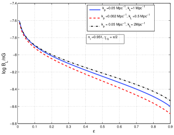
Figure 8: Bounds on the protogalactic field intensity as a function of the magnetic spectral index $\varepsilon$ for different values of the parameters defining the adiabatic contribution to the SW plateau.

In Fig. 8 the scalar spectral index is fixed to $n_{r}=0.951$ wmap3 . In Fig. 9 the two curves corresponding, respectively, to $n_{r}=0.8$ and $n_{r}=1$ are reported.

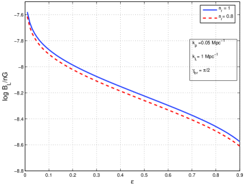
Figure 9: Same plot as in Fig. 8 but with emphasis on the variation of $n_{\rm r}$.

If $\varepsilon<0.2$ the bounds are comparatively less restrictive than in the case $\varepsilon\simeq 0.9$. The cause of this occurrence is that we are here just looking at the largest wavelengths of the problem. As it will become clear in a moment, intermediate scales will be more sensitive to the presence of fully inhomogeneous magnetic fields.

According to Figs. 8 and 9 for a given value of the magnetic spectral index and of the scalar spectral index the amplitude of the magnetic field has to be sufficiently small not to affect the dominant adiabatic nature of the SW plateau. Therefore Figs. 8 and 9 (as well as other similar plots) can be used to normalize the numerical calculations for the power spectra of the brightness perturbations, i.e.

$$\frac{k^{3}}{2\pi^{2}}|\Delta_{\rm I}(k,\tau)|^{2},\qquad\frac{k^{3}}{2\pi^{2}}|\Delta_{\rm P}(k,\tau)|^{2},\qquad\frac{k^{3}}{2\pi^{2}}|\Delta_{\rm I}(k,\tau)\Delta_{\rm P}(k,\tau)|.$$ (215)

Let us then assume, for consistency with the cases reported in Figs. 8 and 9, that we are dealing with the situation where the magnetic field is not correlated with the adiabatic mode. It is then possible to choose a definite value of the magnetic spectral index (for instance $\epsilon=0.1$) and a definite value of the adiabatic spectral index, i.e. $n_{r}$ (for instance $n_{r}=0.951$, in agreement with wmap3 ). By using the SW plateau the normalization can be chosen in such a way the the adiabatic mode dominates over the magnetic contribution. In the mentioned case, Fig. 8 implies $B_{L}<1.14\times 10^{-8}\,\,{\rm G}$ for a pivot scale $k_{p}=0.002\,{\mathrm{Mpc}}^{-1}$. Since the relative weight of the power spectra given in Eqs. (187) and (188) is fixed, it is now possible to set initial conditions for the adiabatic mode according to Eqs. (161)–(163), (164)–(166) and (169) deep in the radiation-dominated phase. The initial time of integration will be chosen as $\tau_{\rm i}=10^{-6}\tau_{1}$ in the notations discussed in Eq. (178). According to Eq. (179), this choice implies that $\tau_{\rm i}\ll\tau_{\rm eq}$.

The power spectra of the brightness perturbations, i.e. Eq. (215), can be then computed by numerical integration. Clearly the calculation will depend upon the values of $\omega_{\rm m}$, $\omega_{\rm b}$, $\omega_{\rm c}$ and $R_{\nu}$. We will simply fix these parameters to their fiducial values reported in Eqs. (181) (see also (147)) and we will take $N_{\nu}=3$ in Eq. (162) determining, in this way the fractional contribution of the neutrinos to the radiation plasma.

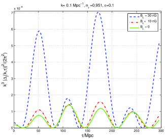
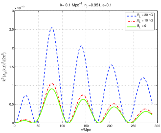
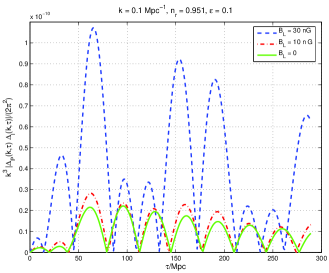
Figure 10: The power spectra of the brightness perturbations for a typical wave-number $k=0.1{\mathrm{M}pc}^{-1}$. The values of the parameters are specified in the legends. The pivot scale is $k_{\rm p}=0.002\,\,{\mathrm{M}pc}^{-1}$ and the smoothing scale is $k_{L}={\mathrm{Mpc}}^{-1}$ (see Figs. 8 and 9).

The first interesting exercise, for the present purposes, is reported in Fig. 10 where the power spectra of the brightness perturbations are illustrated for a wave-number $k=0.1\,\,{\mathrm{M}pc}^{-1}$. Concerning the results reported in Fig. 10 different comments are in order:

• for $\varepsilon=0.1$ and $n_{r}=0.951$, the SW plateau imposes $B_{L}<1.14\times 10^{-8}\,\,{\mathrm{G}}$; from Fig. 10 it follows that a magnetic field of only $30\,\,{\rm nG}$ (i.e. marginally incompatible with the SW bound) has a large effect on the brightness perturbations as it can be argued by comparing, in Fig. 10, the dashed curves (corresponding to $30\,\,{\rm nG}$ ) to the full curves which illustrate the case of vanishing magnetic fiels;

• the situation where $B_{L}>{\mathrm{n}G}$ cannot be simply summarized by saying that the amplitudes of the power spectra get larger since there is a combined effect which both increases the amplitudes and shifts slightly the phases of the oscillations;

• from the qualitative point of view, it is still true that the intensity oscillates as a cosine, the polarization as a sine;

• the phases of the cross-correlations are, comparatively, the most affected by the presence of the magnetic field.

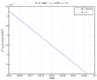
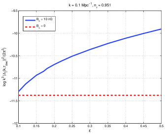
Figure 11: A detail of the cross-correlation (top). The autocorrelation of the intensity at $\tau_{\rm dec}$ as a function of $\varepsilon$, i.e. the magnetic spectral index (bottom).

The features arising in Fig. 10 can be easily illustrated for other values of $\epsilon$ and for different choices of the pivot or smoothing scales. The general lesson that can be drawn is that the constraint derived only by looking at the SW plateau are only a necessary condition on the strength of the magnetic field. They are, however, not sufficient to exclude observable effects at smaller scales. This aspect is illustrated in the plot at the left in Fig. 11 which captures a detail of the cross-correlation. The case when $B_{L}=0$ can be still distinguished from the case $B_{L}=0.5\,\,{\mathrm{n}G}$. Therefore, recalling that for the same choice of parameters the SW plateau implied that $B_{L}<11.4\,\,{\mathrm{n}G}$, it is apparent that the intermediate scales lead to more stringent conditions even for nearly scale-invariant spectra of magnetic energy density. For the range of parameters of Fig. 11 we will have that $B_{L}<0.5\,\,{\mathrm{n}G}$ which is more stringent than the condition deduced from the SW plateau by, roughly, one order of magnitude.

If $\varepsilon$ increases to higher values (but always with $\varepsilon<0.5$) by keeping fixed $B_{L}$ (i.e. the strength of the magnetic field smoothed over a typical length scale $L=2\pi/k_{L}$) the amplitude of the brightness perturbations gets larger in comparison with the case when the magnetic field is absent. This aspect is illustrated in the bottom plot of Fig. 11 where the logarithm (to base $10$) of the intensity autocorrelation is evaluated at a fixed wave-number (and at $\tau_{\rm dec}$) as a function of $\varepsilon$. The full line (corresponding to a $B_{L}=10\,\,{\mathrm{n}G}$) is progressively divergent from the dashed line (corresponding to $B_{L}=0$) as $\varepsilon$ increases.

In Fig. 12 the power spectra of the brightness perturbations are reported at $\tau_{\rm dec}$ and as a function of $k$. In the two plots at the top the autocorrelation of the intensity is reported for different values of $B_{L}$ (left plot) and for different values of $\varepsilon$ at fixed $B_{L}$ (right plot). In the two plots at the bottom the polarization power spectra are reported always at $\tau_{\rm dec}$ and for different values of $B_{L}$ at fixed $\varepsilon$. The position of the first peak of the autocorrelation of the intensity is, approximately, $k_{\rm d}\simeq 0.017\,\,{\mathrm{M}pc}^{-1}$. The position of the first peak of the cross-correlation is, approximately, $3/4$ of $k_{\rm d}$. From this consideration, again, we can obtain that $B_{L}<0.3\,\,{\mathrm{n}G}$ which is more constraining than the SW condition.

Up to now the adiabatic mode has been considered in detail. We could easily add, however, non-adiabatic modes that are be partially correlated with the adiabatic mode. It is rather plausible, in this situation, that by adding new parameters, also the allowed value of the magnetic field may increase. Similar results can be achieved by deviating from the assumption that the magnetic field and the curvature perturbations are uncorrelated. This aspect can be understood already from the analytical form of the SW plateau (192). If there is no correlation between the magnetized contribution and the adiabatic contribution, i.e. $\gamma_{br}=\pi/2$, the SW plateau will be enhanced in comparison with the case when magnetic fields are absent. The same situation arises when the two components are anti-correlated (i.e. $\cos{\gamma_{br}}<0$). However, if the fluctuations are positively correlated (i.e. $\cos{\gamma_{br}}>0$) the cross-correlation adds negatively to the sum of the two autocorrelations of ${\mathcal{R}}$ and $\Omega_{\rm B}$ so that the total result may be an overall reduction of the power with respect to the case $\gamma_{br}=\pi/2$.

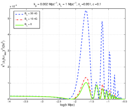
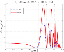
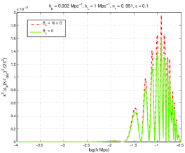
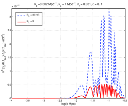
Figure 12: The power spectra of the brightness perturbations at $\tau_{\rm dec}$ for the parameters reported in the legends.

From Fig. 12 various features can be appreciated. The presence of magnetic fields, as already pointed out, does not affect only the amplitude but also the phases of oscillations of the various brightness perturbations. Moreover, an increase in the spectral index $\varepsilon$ also implies a quantitative difference in the intensity autocorrelation.

5 Concluding remarks

There is little doubts that large-scale magnetic exist in nature. These fields have been observed in a number of different astrophysical systems. The main question concerns therefore their origin. String cosmological models of pre-big bang type still represent a viable and well motivated theoretical option.

Simple logic dictates that if the origin of the large-scale magnetic fields is primordial (as opposed to astrophysical) it is plausible to expect the presence of magnetic fields in the primeval plasma also before the decoupling of radiation from matter. CMB anisotropies are germane to several aspect of large-scale magnetization. CMB physics may be the tool that will finally enable us either to confirm or to rule out the primordial nature of galactic and clusters magnetic fields seeds. In the next five to ten years the forthcoming CMB precision polarization experiments will be sensitive in, various frequency channels between 30 GHz and, roughly 900 GHz. The observations will be conducted both via satellites (like the Planck satellite) and via ground based detectors (like in the case of the QUIET arrays). In a complementary view, the SKA telescope will provide full-sky surveys of Faraday rotation that may even get close to 20 GHz.

In an optimistic perspective the forthcoming experimental data together with the steady progress in the understanding of the dynamo theory will hopefully explain the rationale for the ubiquitous nature of large-scale magnetization. In a pessimistic perspective, the primordial nature of magnetic seeds will neither be confirmed nor ruled out. It is wise to adopt a model-independent approach by sharpening those theoretical tools that may allow, in the near future, a direct observational test of the effects of large-scale magnetic fields on CMB anisotropies. Some efforts along this perspective have been reported in the present lecture. In particular, the following results have been achieved:

• scalar CMB anisotropies have been described in the presence of a fully inhomogeneous magnetic field;

• the employed formalism allows the extension of the usual CMB initial conditions to the case when large-scale magnetic fields are present in the game;

• by going to higher order in the tight coupling expansion the evolution of the brightness perturbations has been computed numerically;

• it has been shown that the magnetic fields may affect not only the amplitude but also the relative phases of the Doppler oscillations;

• from the analysis of the cross-correlation power spectra it is possible to distinguish, numerically, the effects of a magnetic field as small as $0.5\,\,\mathrm{n\,G}$.

It is interesting to notice that a magnetic field in the range $10^{-10}$–$10^{-11}$ G is still viable according to the present considerations. It is, therefore, not excluded that large-scale magnetic fields may come from a primordial field of the order of $0.1$-$0.01$ nG present prior to gravitational collapse of the protogalaxy. Such a field, depending upon the details of the gravitational collapse may be amplified to the observable level by compressional amplification. The present problems in achieving a large dynamo amplification may therefore be less relevant than for the case when the seed field is in the range $10^{-9}\mathrm{nG}=10^{-18}\mathrm{nG}$. To confirm this type of scenario it will be absolutely essential to introduce the magnetic field background into the current strategies of parameter extraction.

The considerations reported in the present lecture provide already the framework for such an introduction. In particular, along a minimalist perspective, the inclusion of the magnetic field background boils down to add two new extra-parameters: the spectral slope and amplitude of the magnetic field (conventionally smoothed over a typical comoving scale of Mpc size). The magnetic field contribution will then slightly modify the adiabatic paradigm by introducing, already at the level of initial conditions, a subleading non-Gaussian (and quasi-adiabatic) correction.

References

- (1) H. Alfvén : Arkiv. Mat. F. Astr., o. Fys. 29 B, 2 (1943).
- (2) E. Fermi: Phys. Rev. 75, 1169 (1949).
- (3) H. Alfvén: Phys. Rev. 75, 1732 (1949).
- (4) R. D. Richtmyer, E. Teller: Phys. Rev. 75, 1729 (1949).
- (5) W. A. Hiltner: Science 109, 165 (1949).
- (6) J. S. Hall: Science 109, 166 (1949).
- (7) L. J. Davis J. L. Greenstein: Astrophys. J. 114, 206 (1951).
- (8) E. Fermi, S. Chandrasekar: Astrophys. J. 118, 113 (1953).
- (9) E. Fermi, S. Chandrsekar: Astrophys. J. 118, 116 (1953).
- (10) R. Wielebinski, J. Shakeshaft: Nature195, 982 (1962).
- (11) A. G. Lyne, F. G. Smith: Nature 218, 124 (1968).
- (12) A. G. Lyne, F. G. Smith: Pulsar Astronomy, (Cambridge University Press, Cambridge, UK, 1998).
- (13) C. Heiles: Annu. Rev. Astron. Astrophys. 14, 1 (1976).
- (14) P. P. Kronberg: Rep. Prog. Phys. 57, 325 (1994).
- (15) F. Govoni, L. Feretti : Int. J. Mod. Phys. D 13, 1549 (2004).
- (16) B.M. Gaensler, R. Beck, L. Feretti: New Astron. Rev. 48, 1003 (2004).
- (17) Y. Xu, P. P. Kronberg, S. Habib, Q. W. Dufton: Astrophys. J. 637, 19 (2006).
- (18) P. P. Kronberg : Astron. Nachr. 327, 517 (2006).
- (19) M. Giovannini: Int. J. Mod. Phys. D 13, 391 (2004).
- (20) See http://www.skatelescope.org for more informations.
- (21) See http://www.rssd.esa.int for more informations.
- (22) M. Giovannini: Class. Quant. Grav. 23, R1 (2006).
- (23) J. Bernstein, L. S. Brown and G. Feinberg: Rev. Mod. Phys. 61, 25 (1989).
- (24) T. J. M Boyd, J. J. Serson: The physics of plasmas, (Cambridge University Press, Cambridge, UK, 2003).
- (25) N. A. Krall, A. W. Trivelpiece: Principles of Plasma Physics, (San Francisco Press, San Francisco 1986).
- (26) F. Chen: Introduction to Plasma Physics, (Plenum Press, New York 1974).
- (27) D. Biskamp: Non-linear Magnetohydrodynamics (Cambridge University Press, Cambridge, 1994).
- (28) A. Vlasov: Zh. Éksp. Teor. Fiz. 8, 291 (1938); J. Phys. 9, 25 (1945).
- (29) L. D. Landau: J. Phys. U.S.S.R. 10, 25 (1945).
- (30) M. Giovannini: Phys. Rev. D 71, 021301 (2005).
- (31) M. Giovannini: Phys. Rev. D 58, 124027 (1998).
- (32) E. N. Parker: Cosmical Magnetic Fields (Clarendon Press, Oxford, 1979).
- (33) Ya. B. Zeldovich, A. A. Ruzmaikin, D.D. Sokoloff: Magnetic Fields in Astrophysics (Gordon Breach Science, New York, 1983).
- (34) A. A. Ruzmaikin, A. M. Shukurov, D. D. Sokoloff : Magnetic Fields of Galaxies, (Kluwer Academic Publisher, Dordrecht, 1988).
- (35) R. Kulsrud: Annu. Rev. Astron. Astrophys. 37, 37 (1999).
- (36) A. Lazarian, E. Vishniac, J. Cho: Astrophys. J. 603, 180 (2004); Lect. Notes Phys. : 614, 376 (2003).
- (37) A. Brandenburg, K. Subramanian: Phys. Rept. 417, 1 (2005).
- (38) A. Brandenburg, A. Bigazzi, K. Subramanian: Mon. Not. Roy. Astron. Soc. 325, 685 (2001).
- (39) K. Subramanian, A. Brandenburg: Phys. Rev. Lett. 93, 205001 (2004).
- (40) A. Brandenburg, K. Subramanian: Astron. Astrophys. 439, 835 (2005).
- (41) S. I. Vainshtein, Ya. B. Zeldovich: Usp. Fiz. Nauk. 106, 431 (1972).
- (42) W. H. Matthaeus, M. L. Goldstein, S. R. Lantz: Phys. Fluids 29, 1504 (1986).
- (43) M. J. Rees: Lect. Notes Phys. 664, 1 (2005).
- (44) K. Subramanian, D. Narashima, S. Chitre: Mon. Not. Roy. Astron. Soc. 271, L15 (1994).
- (45) N. Y. Gnedin, A. Ferrara, E. G. Zweibel: Astrophys. J. 539, 505 (2000).
- (46) R. Kulsrud, S. erson: Astrophys. J. 396, 606 (1992).
- (47) Ya. Zeldovich, I. Novikov: The structure evolution of the Universe (Chicago University Press, Chicago, 1971), Vol. 2.
- (48) Ya. Zeldovich: Sov. Phys. JETP 21, 656 (1965).
- (49) E. Harrison: Phys. Rev. Lett. 18, 1011 (1967).
- (50) E. Harrison: Phys. Rev. 167, 1170 (1968).
- (51) E. Harrison: Mon. Not. R. Astr. Soc. 147, 279 (1970).
- (52) L. Biermann: Z. Naturf. 5A, 65 (1950).
- (53) I. Mishustin, A. Ruzmaikin: Sov. Phys. JETP 34, 223 (1972).
- (54) M. Giovannini: Phys. Rev. D 61, 063004 (2000).
- (55) M. Giovannini: Phys. Rev. D 61, 063502 (2000).
- (56) G. Piccinelli, A. Ayala: Lect. Notes Phys. 646, 293 (2004).
- (57) D. Boyanovsky, H. J. de Vega, M. Simionato: Phys. Rev. D 67, 123505 (2003).
- (58) D. Boyanovsky, M. Simionato, H. J. de Vega: Phys. Rev. D 67, 023502 (2003).
- (59) M. Giovannini, M. E. Shaposhnikov, Phys. Rev. D 57, 2186 (1998).
- (60) K. Bamba: arXiv:hep-ph/0611152.
- (61) A. Sanchez, A. Ayala, G. Piccinelli: arXiv:hep-th/0611337.
- (62) M. Giovannini, M. E. Shaposhnikov: Phys. Rev. D 62, 103512 (2000).
- (63) M. Giovannini, M. Shaposhnikov: Proc. of CAPP2000 (July 2000, Verbier Switzerland) eprint Archive [hep-ph/0011105].
- (64) E. Calzetta, A. Kus, F. Mazzitelli: Phys. Rev. D, 57, 7139 (1998).
- (65) A. Kus, E. Calzetta, F. Mazzitelli, C. Wagner: Phys.Lett. B 472, 287 (2000).
- (66) M. S. Turner, L. M. Widrow: Phys. Rev. D 37, 2734 (1988).
- (67) B. Ratra: Astrophys. J. Lett. 391, L1 (1992).
- (68) A. Dolgov: Phys. Rev. D 48, 2499 (1993).
- (69) I. Drummond, S. Hathrell: Phys.Rev. D 22, 343 (1980).
- (70) S. Carroll, G. Field, R. Jackiw: Phys. Rev. D 41, 1231 (1990).
- (71) W. D. Garretson, G. Field, S. Carroll: Phys. Rev. D 46, 5346 (1992).
- (72) G. Field, S. Carroll Phys. Rev. D: 62, 103008 (2000).
- (73) M. Giovannini: Phys. Rev. D 64, 061301 (2001).
- (74) K. Bamba, J. Yokoyama, e-print Archive [astro-ph/0310824].
- (75) M. Gasperini, Phys. Rev. D 63, 047301 (2001)
- (76) L. Okun, Sov. Phys. JETP 56, 502 (1982).
- (77) O. Bertolami D. Mota, Phys. Lett. B 455, 96 (1999).
- (78) M. Giovannini, Phys. Rev. D 62, 123505 (2000).
- (79) L. H. Ford, Phys.Rev. D 31, 704 (1985).
- (80) M. Gasperini, M. Giovannini, G. Veneziano: Phys. Rev. Lett. 75, 3796 (1995).
- (81) M. Gasperini, M. Giovannini, G. Veneziano: Phys. Rev. D 52, 6651 (1995).
- (82) M. Gasperini, M. Giovannini: Phys. Rev. D 47, 1519 (1993).
- (83) H. Yuen: Phys. Rev. A 13, 2226 (1976).
- (84) A. O. Barut, L. Girardello: Commun. Math. Phys. 21, 41 (1971).
- (85) D. Stoler: Phys. Rev. D 1, 3217 (1970); D. Stoler: Phys. Rev. D 4, 2309 (1971).
- (86) S. Fubini, A. Molinari: Nucl. Phys. Proc. Suppl. 33C, 60 (1993).
- (87) R. Loudon: J. Mod. Opt. 34, 709 (1987).
- (88) R. Loudon: The quantum theory of light (Clarendon Press, Oxford, 1983).
- (89) B. L. Schumaker: Phys. Rept. 135, 318 (1986).
- (90) L. Mandel, E. Wolf: Optical coherence and quantum optics, (Cambridge University Press, Cambridge UK, 1995).
- (91) G. Veneziano: Phys. Lett. B 265, 287 (1991).
- (92) M. Gasperini, G. Veneziano: Astropart. Phys. 1, 317 (1993).
- (93) M. Gasperini, G. Veneziano: Phys. Rept. 373, 1 (2003).
- (94) C. Lovelace: Phys. Lett. B 135, 75 (1984).
- (95) E. Fradkin, A. Tseytlin: Nucl. Phys. B 261, 1 (1985)
- (96) C. Callan at al.: Nucl. Phys. B 262, 593 (1985).
- (97) M. Gasperini, M. Giovannini, G. Veneziano: Phys. Lett. B 569, 113 (2003).
- (98) M. Gasperini, M. Giovannini, G. Veneziano: Nucl. Phys. B 694, 206 (2004).
- (99) K. A. Meissner, G. Veneziano: Mod. Phys. Lett. A 6, 3397 (1991).
- (100) K. A. Meissner G. Veneziano: Phys. Lett. B 267, 33 (1991).
- (101) M. Gasperini, J. Maharana, G. Veneziano: Nucl. Phys. B 472, 349 (1996).
- (102) M. Giovannini: Class. Quant. Grav. 21, 4209 (2004).
- (103) M. Gasperini, M. Giovannini: Phys. Rev. D 47, 1519 (1993).
- (104) M. Gasperini, M. Giovannini: Phys. Lett. B 301, 334 (1993).
- (105) M. Giovannini: Phys. Rev. D 61, 087306 (2000).
- (106) R. Brustein, M. Gasperini, M. Giovannini, G. Veneziano, Phys. Lett. B 361, 45 (1995).
- (107) R. Brustein, M. Gasperini, M. Giovannini, V. F. Mukhanov, G. Veneziano, Phys. Rev. D 51, 6744 (1995).
-
(108)
K. Enqvist M. S. Sloth:
Nucl. Phys. B 626, 395 (2002);
M. S. Sloth: Nucl. Phys. B 656, 239 (2003). -
(109)
V. Bozza, M. Gasperini, M. Giovannini, G. Veneziano:
Phys. Rev. D 67 (2003) 063514.
V. Bozza, M. Gasperini, M. Giovannini, G. Veneziano: Phys. Lett. B 543, 14 (2002). - (110) P. Astone et al.: Astron. Astrophys. 351, 811 (1999).
- (111) Ph. Bernard, G. Gemme, R. Parodi, E. Picasso: Rev. Sci. Instrum. 72, 2428 (2001).
-
(112)
A. M. Cruise: Class. Quantum Grav. 17, 2525 (2000);
A. M. Cruise: Mon. Not. R. Astron. Soc 204, 485 (1983). -
(113)
D. Babusci and M. Giovannini:
Int.J. Mod. Phys. D 10 477 (2001);
D. Babusci and M. Giovannini: Class. Quant. Grav. 17, 2621 (2000). - (114) P. J. E. Peebles, A. Vilenkin: Phys. Rev. D 59, 063505 (1999).
-
(115)
M. Giovannini: Class. Quant. Grav. 16, 2905 (1999);
M. Giovannini: Phys. Rev. D 60, 123511 (1999).
D. Babusci and M. Giovannini: Phys. Rev. D 60, 083511 (1999);
M. Giovannini: Phys. Rev. D 58, 083504 (1998). - (116) M. Gasperini, S. Nicotri: e-print [hep-th/0511039].
- (117) R. Beck: Astron.Nachr. 327, 512 (2006).
- (118) R. Beck, A. Brenburg, D. Moss, A. Skhurov, D. Sokoloff: Annu. Rev. Astron. Astrophys. 34, 155 (1996).
- (119) J. Vallée: Astrophys. J. 566, 261 (2002).
- (120) E. Battaner, E. Florido: Mon. Not. R. Astron. Soc 277, 1129 (1995).
- (121) E. Battaner, E. Florido, J. Jimenez-Vincente: Astron.Astrophys. 326, 13 (1997).
- (122) E. Florido, E. Battaner: Astron.Astrophys. 327, 1 (1997).
- (123) E. Florido, et al.: arXiv:astro-ph/0609384.
- (124) E. Battaner, E. Florido, Fund. Cosmic Phys. 21, 1 (2000).
- (125) K. Subramanian: Astron.Nachr. 327, 399 (2006).
- (126) M. Giovannini: Class. Quant. Grav. 23, R1 (2006).
-
(127)
A. Brandenburg, K. Subramanian:
Phys. Rept. 417, 1 (2005);
A. Lazarian, E. Vishniac, J. Cho: Astrophys. J. 603, 180 (2004); Lect. Notes Phys. 614, 376 (2003). -
(128)
J. Barrow, K. Subramanian: Phys. Rev. Lett. 81,
3575 (1998);
J. Barrow, K. Subramanian: Phys. Rev. D 58, 83502 (1998);
C. Tsagas, R. Maartens: Phys. Rev. D 61, 083519 (2000);
A. Mack, T. Kahniashvili, A. Kosowsky: Phys. Rev. D 65, 123004 (2002);
A. Lewis: Phys. Rev. D 70, 043518 (2004);
T. Kahniashvili, B. Ratra: Phys. Rev. D 71, 103006 (2005). -
(129)
G. Chen et al.:
Astrophys. J. 611, 655 (2004);
P. D. Naselsky et al.: Astrophys. J. 615, 45 (2004); L. Y. Chiang, P. Naselsky: Int. J. Mod. Phys. D 14, 1251 (2005);
L. Y. Chiang, P. D. Naselsky, O. V. Verkhodanov, M. J. Way: Astrophys. J. 590, L65 (2003);
D. G. Yamazaki et al.: Astrophys. J. 625, L1 (2005). - (130) H. V. Peiris et al., [WMAP Collaboration]: Astrophys. J. Suppl. 148, 213 (2003).
- (131) D. Spergel et al. [WMAP Collaboration]: arXiv:astro-ph/0603449.
- (132) K. Enqvist, H. Kurki-Suonio J. Valiviita: Phys. Rev. D 62, 103003 (2000).
- (133) H. Kurki-Suonio, V. Muhonen J. Valiviita: Phys. Rev. D 71, 063005 (2005).
- (134) K. Moodley, M. Bucher, J. Dunkley, P. G. Ferreira C. Skordis: Phys. Rev. D 70, 103520 (2004).
- (135) M. Giovannini: Phys. Rev. D 73, 101302 (2006).
- (136) M. Giovannini: Phys. Rev. D 74, 063002 (2006).
- (137) M. Giovannini: Class. Quant. Grav. 23, 4991 (2006).
- (138) J. D. Barrow, R. Maartens, C. G. Tsagas: arXiv:astro-ph/0611537.
- (139) T. Kahniashvili, B. Ratra: arXiv:astro-ph/0611247.
- (140) E. Harrison: Rev. Mod. Phys. 39, 862 (1967).
- (141) J. M. Bardeen: Phys. Rev. D 22, 1882 (1980).
- (142) C.-P. Ma E. Bertschinger: Astrophys. J. 455, 7 (1995).
- (143) M. Giovannini: Phys. Rev. D 70, 123507 (2004).
- (144) M. Giovannini: Int. J. Mod. Phys. D 14, 363 (2005).
- (145) M. Giovannini: Phys. Rev. D 71, 021301 (2005).
- (146) J. Bardeen, P. Steinhardt, M. Turner: Phys. Rev. D 28, 679 (1983).
- (147) R. Brandenberger, R. Kahn, W. Press: Phys. Rev. D 28, 1809 (1983).
- (148) M. Giovannini: Phys. Lett. B 622, 349 (2005).
- (149) M. Giovannini: Class. Quant. Grav. 22, 5243 (2005).
- (150) W. Hu N. Sugiyama: Astrophys. J. 444, 489 (1995); ibid. 471, 30 (1996).
- (151) H. V. Peiris et al. [WMAP collaboration]: Astrophys. J. Suppl. 148, 213 (2003).
- (152) L. Page et al. [WMAP collaboration]: arXiv:astro-ph/0603450.
- (153) A. G. Riess et al., Astrophys. J. 607, 665 (2005).
- (154) P. Astier et al., astro-ph/0510447.
- (155) P. Naselsky, I. Novikov: Astrophys. J. 413, 14 (1993).
- (156) H. Jorgensen, E. Kotok, P. Naselsky, I Novikov: Astron. Astrophys. 294, 639 (1995).
- (157) P. J. E. Peebles, J. T. Yu: Astrophys. J. 162, 815 (1970).
- (158) A. G. Doroshkevich, Ya. B. Zeldovich, R. A. Sunyaev: Sov. Astron. 22, 523 (1978).
- (159) M. Zaldarriaga D. D. Harari: Phys. Rev. D 52 (1995) 3276.
- (160) S. Chandrasekar: Radiative Transfer, (Dover, New York, US, 1966).