Large Structures and Galaxy Evolution in COSMOS at z $<1.1$

Abstract

We present the first identification of large-scale structures (LSS) at z $<1.1$ in the Cosmic Evolution Survey (COSMOS). The structures are identified from adaptive smoothing of galaxy counts in the pseudo-3d space ($\alpha,\delta$,z) using the COSMOS photometric redshift catalog. The technique is tested on a simulation including galaxies distributed in model clusters and a field galaxy population – recovering structures on all scales from 1 to 20′ without a priori assumptions for the structure size or density profile. Our procedure makes no a priori selection on galaxy spectral energy distribution (SED, for example the Red Sequence), enabling an unbiased investigation of environmental effects on galaxy evolution.

The COSMOS photometric redshift catalog yields a sample of $1.5\times 10^{5}$ galaxies with redshift accuracy, $\Delta z_{FWHM}/(1+z)\leq 0.1$ at z $<1.1$ down to I${}_{AB}\leq 25$ mag. Using this sample of galaxies, we identify 42 large-scale structures and clusters. Projected surface-density maps for the structures indicate multiple peaks and internal structure in many of the most massive LSS. The stellar masses (determined from the galactic SEDs) for the LSS range from M${}_{*}\sim 10^{11}$ up to $\sim 3\times 10^{13}$ $M_{\odot}$. Five LSS have total stellar masses exceeding $10^{13}$ $M_{\odot}$. (Total masses including non-stellar baryons and dark matter are expected to be $\sim 50\rightarrow 100$ times greater.) The derived mass function for the LSS is consistent (within the expected Poisson and cosmic variances) with those derived from optical and X-ray studies at lower redshift.

To characterize structure evolution and for comparison with simulations, we compute a new statistic – the area filling factor as a function of the overdensity value compared to the mean at surface overdensity ($f_{A}(\Sigma/{\overline{\Sigma}(z)}$). The observationally determined f_A has less than 1% of the surface area (in each redshift slice) with overdensities exceeding 10:1 and evolution to higher overdensities is seen at later epochs (lower z) – both characteristics are in good agreement with what we find using similar processing on the Millennium Simulation. Although similar variations in the filling factors as a function of overdensity and redshift are seen in the observations and simulations, we do find that the observed distributions reach higher overdensity than the simulation, perhaps indicating over-merging in the simulation.

All of the LSS show a dramatic preference for earlier spectral energy distribution (SED type) galaxies in the denser regions of the structures, independent of redshift. The SED types in the central 1 Mpc and 1 – 5 Mpc regions of each structure average about 1 SED type earlier than the mean type at the same redshift, corresponding to a stellar population age difference of $\sim$2 – 4 billion years at z = 0.3 to 1.

We also investigate the evolution of key galactic properties – mass, luminosity, SED and star formation rate (SFR) – with redshift and environmental density as derived from overdensities in the full pseudo 3-d cube. Both the maturity of the stellar populations and the ’downsizing’ of SF in galaxies vary strongly with redshift (epoch) and environment. For a very broad mass range (10${}^{10}--10^{12}$$M_{\odot}$), we find that galaxies in dense environments tend to be older – this is not just restricted to the most massive galaxies. And in low density environments, the most massive galaxies appear to have also been formed very early (z $>2$), compared to the lower mass galaxies there. Over the range z $<1.1$, we do not see evolution in the mass of galaxies by more than a factor $\sim 2$ separating active and inactive star-forming galaxy populations.

1 Introduction

The Cosmic Evolution Survey (COSMOS) is intended to probe the evolution of galaxies, AGN and dark matter in the context of their cosmic environment (large-scale structure – LSS). The survey area samples scales of LSS out to $\sim$ 50 – 100 Mpc at z $>0.5$. This corresponds to 9 times the area of GEMS and EGS (Rix et al., 2004; Davis et al., 2006), the next largest HST imaging surveys. The COSMOS area (Scoville, 2006a) is expected to have a 50% probability of having one 10¹⁴ $M_{\odot}$ halo (dark and luminous matter) within every $\Delta$z $\sim$ 0.1 at z $\sim$ 1 – 2 (based on $\Lambda$CDM simulations; see Benson et al. (2001)); lower mass halos ($\sim 10^{13}$ $M_{\odot}$) are $\sim 20$ times more abundant and therefore will be seen in every $\Delta$z $\sim$ 0.1. A major theme for COSMOS is the effect of cosmological environment on the evolution of galaxies and AGN. The identification and measurement of LSS are therefore a prerequisite to many aspects of science with COSMOS since the large-scale structures define the local environment. In COSMOS, the local galaxy number and mass densities can be compared with the total mass densities determined from weak lensing tomography and hot X-ray emitting gas in the virialized parts of LSS having clusters of galaxies (see below, Massey, 2006; Finoguenov et al., 2006).

The identification of LSS from the observed surface-density of galaxies requires some means of discriminating galaxies at different distances along the line of sight; otherwise, the increased shot noise in the galaxy counts reduces the signal-to-noise ratio for the large-scale structure. The better the redshift or distance discrimination, the easier it is to see low density, large-scale structures. (This is true down to the point that the internal velocity dispersion of the structure is resolved.) For LSS finding, line-of-sight discrimination is usually accomplished using: 1) color selection (e.g. using broadband colors to select red sequence galaxies, Gladders & Yee, 2005); 2) photometric redshifts based on the broadband spectral energy distribution (SED), or 3) spectroscopic redshifts (see Appendix A; van de Weygaert, 1994; Postman et al., 1996; Schuecker & Boehringer, 1998; Marinoni et al., 2002). Color selection is not used here since it would preclude investigation of correlations between environmental density and galaxy SED or morphological type (Dressler et al., 1997; Smith et al., 2005). With color selection, the defined large-scale structures would be a priori biased to a particular galactic SED type (e.g. early type galaxies if the red-sequence method is used). High density structures may well be rich in red galaxies of early morphological type, but exploring the dependence of galaxy type on environmental density requires that the environment be defined or identified without bias toward specific galaxy types. Ultimately, the use of spectroscopic redshifts to determine distances is more desirable, provided a sufficiently large sample exists (Le Fèvre et al., 2005; Gerke et al., 2005; Meneux et al., 2006; Cooper et al., 2006; Coil et al., 2006). The z-COSMOS spectroscopic survey will yield $\sim$ 30,000 galaxies when completed in $\sim$2008 (Lilly, 2006; Impey, 2006); however, at this time the spectroscopy is much more limited and we must rely on the alternative approaches for line-of-sight discrimination.

In this paper, we identify LSS in the 2□^∘COSMOS field using the extensive COSMOS photometric redshift catalog (Mobasher et al., 2006) to analyze the galaxy surface density in redshift slices out to z = 1.2. The galaxy samples used for this work and their completeness are discussed in Section 2. We use an adaptive smoothing technique (see Appendix A) to identify areas of significantly enhanced galaxy surface-density. For each significant peak in the smoothed surface-density pseudo 3-d cube, we find all connected pixels to delineate a sample of 42 structures (Section 3). For each structure, we estimate the dimensions, number of galaxies, and mass (from the broadband fluxes of the galaxies). The stellar mass distribution of identified COSMOS LSS extends from 10¹¹ up to $3\times 10^{13}$ $M_{\odot}$. The relative amount of structure at different overdensities is analysed in Section 4 and compared with results from the Millennium Simulation.

We then investigate the evolution of galaxies with respect to their location in the 42 LSS in Section 5 and environmental density in Section 6. Strong variation of the SED type and star formation activity is seen with both redshift and environmental density. The maturity of the stellar populations and the ’downsizing’ of SF in galaxies is also strongly varying with epoch and environment (Section 6.4.3). (Adopted cosmological parameters, used throughout, are: H₀ = 70 km s^-1 Mpc^-1, $\Omega_{M}$ = 0.3 and $\Omega_{\Lambda}$ = 0.7)

2 Photometric Redshifts and Sample Selection

For this investigation we use photometric redshifts to separate the galaxy population along the line-of-sight. It is vital for the analysis that the binning in redshift be matched to the accuracy of the redshifts. Using binning that is finer than the redshift uncertainties distributes the galaxies in a single structure over multiple redshift slices and thus reduces the signal in each slice. Conversely, bins of width larger than the redshift uncertainties will increase the shot noise associated with the background surface-density of galaxies, relative to the large-scale structure signal.

The COSMOS photometry catalogs were generated from deep ground-based optical imaging at Subaru (Taniguchi et al., 2006) and CFHT; they are combined with shallower near infrared imaging from NOAO (KPNO and CTIO) (Capak, 2006). The resulting photometric redshift catalog contains 1.2 million objects at I${}_{AB}<$26 (Mobasher et al., 2006). For approximately 900 objects (all with I${}_{AB}\leq 24$ mag from zCOSMOS Lilly (2006)), there exist spectroscopic redshifts; after removing ’catastrophic’ outliers ($\sim$1% of the sample), the offsets between the photometric and spectroscopic redshifts have $\sigma_{z}/(1+z)\simeq 0.03$ or $\Delta z_{FWHM}/(1+z)\leq 0.1$ (Mobasher et al., 2006). Since the spectroscopic – photometric redshift comparison is limited to a small sample of mostly brighter objects, we will instead use the ’goodness’ of fit from the photometric redshift determination for a more general assessment of the redshift accuracies. This represents an internal dispersion and hence is likely to be lower than the true uncertainty which includes systematic effects; nevertheless, it does provide a characterization of the dependence on redshift and magnitude cutoff for any sample selection.

The photometric redshifts were derived using the Bayesian Photometric Redshift method (BPZ: Benson et al., 2000; Mobasher et al., 2006). The fitting presumes 6 basic spectral energy distributions (SEDs) and for the photometric redshift catalog used here, there was no assumed ’prior distribution’ for the galaxy magnitudes. The dust extinction within each galaxy was also a free parameter in the redshift fitting. For SED types 0 to 2, a Galactic extinction law was assumed: for SED types greater than 2, a Calzetti law was used (Mobasher et al., 2006). The fitting outputs the most probable redshift, 68 and 95% confidence intervals, the intrinsic SED type and the absolute magnitude (M_V). In Figure 1, the redshift distribution and uncertainty in the redshift fits are shown as a function of redshift and i-band magnitude cutoff in the sample. The SED classifications used here are : 1 (E/S0), 2 (Sa/Sb), 3(Sc), 4(Im), and 5-6(starburst). The quantity $\Delta$ z(50%)/(1+z) shown in Figure 1b is the mean value (at each z) of the width in z containing 50% of the probability distribution. (This full-width is 1.3$\times\sigma$ for the derived fits, assuming a Gaussian uncertainty distribution.) Also shown is the photometric redshift uncertainty as a function of apparent magnitude cutoff – based on these curves, we adopt a cutoff $I_{AB}=25$ mag. The uncertainties plotted in Figure 1 indicate that the bin width for identifying large-scale structures should be approximately $\Delta z\simeq 0.1-0.15$ up to z $\simeq 1.2$ and $\Delta z\simeq 0.25$ up to z $\simeq 2.5$ for the chosen magnitude limit.

Throughout the investigation here, we use the galaxy rest frame SEDs to characterize the galaxy type, rather than the observed morphologies. Capak et al. (2006) find a tight correlation between SED and morphology as measured by the Gini and Compactness measures. We have also correlated the Sersic indices measured using GALFIT for 5,000 bright (I $<$ 22 mag) galaxies in COSMOS at z = 0.2 to 0.8. The SED type 1 (E/S0) is strongly correlated with an R^1/4 law (Sersic n = 4); however, there exists a large dispersion in the Sersic indices for the later SED types. This large dispersion probably reflects both the real dispersion in bulge to disk ratios of later galaxy types and the difficulties of measuring the morphologies for faint galaxies at high redshift. Throughout this investigation we will use the SED types, derived from the photometric redshift fitting, to classify the galaxies since the SEDs are more readily classified for faint galaxies than the morphology.

The COSMOS photometric redshift catalog also includes galactic stellar masses, derived from the absolute magnitude, SED type and redshift of each galaxy (Mobasher et al., 2006). Approximate estimates for the star formation rates (SFR) were also derived using the SED type, absolute magnitude and fitted extinction. The intrinsic UV continuum (corrected for extinction at $\lambda=1500$ Å) was used to estimate the SFR (Mobasher, 2006).

2.1 Galaxy Samples

Although the COSMOS photometric redshift catalog contains over a million objects, we impose selection criteria to yield a more reliable galaxy sample for structure identification – i.e. galaxies with the best photometric redshifts, detected in several bands, and with significant intrinsic luminosity. We thus restrict the analysis to :

$$25~{}~{}mag\geq I_{AB}\geq 19~{}~{}mag$$ (1a)

$$M_{V}\leq-18~{}~{}mag$$ (1b)

We also require that each object be detected in at least 4 bands and the SExtractor stellarity parameter be less than 0.95. The former (in addition to the 25 mag cutoff – Eq (1a)) limits the sample to galaxies with accurate photometry; the latter removes objects which are likely to be stars or QSOs. Similarly very bright objects are also excluded by condition (1a) since they are likely to be stars. Since the fraction of galaxies with dominant AGN is probably not large, their exclusion should not significantly affect the large-scale structure definition. Condition (1b) removes galaxies which have low absolute luminosities and presumably low mass. These criteria yield the galaxy samples listed in Table 1 along with the adopted redshift binning for the LSS identifications presented below. In Table 1, we also provide a breakdown of the samples with respect to SED type from the photometric-redshift fitting. The majority of the analysis in this paper refers to the low-z sample in Table 1.

2.2 Galaxy Selection and Completeness with Redshift

At larger redshifts, the galaxy sample used to define LSS will be incomplete at low luminosities (masses) and we evaluate here the severity of this effect with two approaches : evaluating the cutoff $L_{*}$ (the characteristic luminosity at the knee in the Schecter luminosity function) as a function of redshift and comparing the galaxy mass functions as a function of redshift for the sample described in Section 2.1.

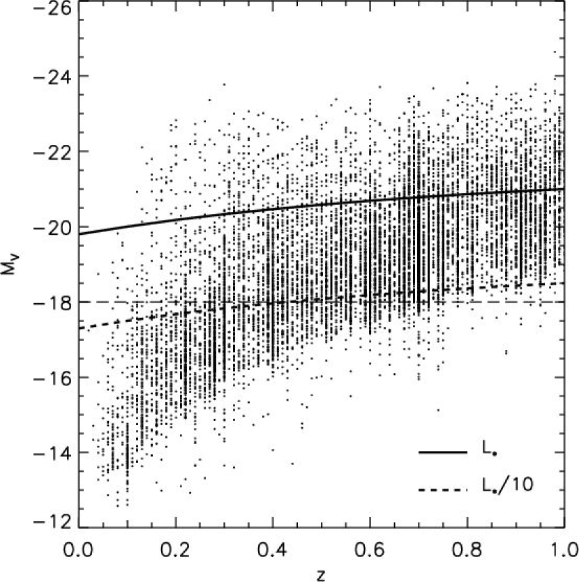
Figure 2: a) Left : The distribution of rest frame M_V for galaxies in our sample is shown as a function of redshift. The lines indicate the expected absolute magnitudes for L_∗ and L${}_{*}/10$ galaxies assuming passive evolution brightening of 1.2 mag from z = 0 to 1. The horizontal line at M${}_{V}=-18$ corresponds to the absolute magnitude cutoff used here. The lower envelope in the grayscale is imposed by our sample cutoff at $I_{AB}<25$ mag. (For clarity only 20,000 randomly sampled galaxies are plotted.) b) Right : The distribution functions of stellar masses for galaxies in our sample with $I_{AB}<25$ mag and M${}_{V}<-18$ are shown for redshift bins of width $\Delta z=0.2$. The higher noise seen in the low z mass functions is due to the much smaller volume and hence smaller number of galaxies sampled; the small falloff seen in the mass functions for z $>0.7$ at M${}_{stellar}<5\times 10^{9}$$M_{\odot}$ is due to the apparent magnitude limit $I_{AB}<25$ mag for our sample.

Figure 2 shows the distributions of absolute magnitude (left) and stellar masses (right) for galaxies in our sample as a function of redshift. On the left panel, the lines indicate the expected absolute magnitudes for L_∗ and L${}_{*}/10$ galaxies assuming a typical, passive evolution brightening of 1.2 mag from z = 0 to 1.2. Here one sees that the sample easily goes down to L${}_{*}/10$ out to z = 1.2 with $I_{AB}<25$ mag (the lower envelope in the grayscale). Incompleteness does set in at less than L${}_{*}/10$, but typically less than 30% of the total luminosity is contained in these galaxies for a Schecter luminosity function.

Alternatively, one can compare the distribution functions of galactic stellar masses as a function of redshift to assess the incompleteness (assuming, to first order, that the mass function is not strongly varying over this redshift interval – e.g. $\leq 2\times$; see Borch et al. (2006) and below). The derived mass functions for galaxies entering the sample (Section 2.1) used here for LSS definition are shown on the right panel of Figure 2. These mass functions are in agreement in both shape and absolute value with previously determined mass functions for this redshift range (Drory et al., 2005; Borch et al., 2006; Bundy et al., 2005). The higher noise seen in the low z mass functions is due to the much smaller volume and hence smaller number of galaxies sampled.

The total number of galaxies and total mass of galaxies per unit comoving volume were evaluated by integrating the distribution functions shown in right panel of Figure 2 at masses above 10⁹ $M_{\odot}$. In columns 2 & 3 of Table 2, the totals are divided by the comoving volume in order to assess the count and mass incompleteness relative to this maximum redshift bin (see Table 2). The falloff seen in the mass functions for z $>0.7$ at M${}_{stellar}<5\times 10^{9}$$M_{\odot}$  is probably due to incompleteness at the apparent magnitude limit $I_{AB}<25$ mag for our sample. Incompleteness at this magnitude limit is quantified for COSMOS in Scoville (2006a). In terms of integrated stellar mass for galaxies above $10^{9}$$M_{\odot}$, our sample is at most missing only 10% (Table 2) of the total mass, relative to the lower redshift bins which are more complete (e.g. z $\sim 0.5$). In the analysis below we will not correct for this incompleteness unless noted explicitly, given the fact that it is probably not large and the uncertain assumptions of constancy in either the mass- or luminosity- function which would be required.

2.3 Pseudo 3-D Surface-Density and Noise Estimates

The adaptive smoothing algorithm we employ here is designed to analyze redshift slices, each of which represents the surface-density of galaxies ($\Sigma$) in a redshift bin. The custom-built algorithm is formally described along with test results in Appendix A. As noted in Section 2, the width of these slices will be $\Delta z=0.1$ and 0.25 for the low and high-z samples respectively. However, given that the different galaxies may have quite different widths for the fitted redshift probability distribution, insertion of each galaxy into the 3-d cube ($\alpha$,$\delta$,z) as a delta function ($\delta(z-z_{pk})$) at the most likely redshift would not optimally weight the galaxies with the most accurate photometric redshifts. Instead, we populate the 3-d cube with a Gaussian distribution in z for each galaxy. The Gaussian dispersion was taken from the high and low-z 68%-confidence limits from the photometric redshift fit – specifically $\sigma_{z}=(z_{high~{}68\%}-z_{low~{}68\%})/2$). Thus, in the adaptive smoothing procedure, galaxies which have a large uncertainty in their derived redshifts will have relatively low weight, because they will be spread over a larger range in the redshift dimension. And galaxies with tighter redshift fits will be treated more significantly. One concern might be that this tends to prefer structures defined by early type galaxies which have a strong Balmer break and thus small redshift uncertainty. As a test, we also used the adaptive smoothing on a 3-d cube with the galaxies located as points (rather than a probability distribution) at their most probable redshift, Since this test yielded structures similar to those shown here, we prefer employ the probability distributions to take account of the redshift uncertainties. The cube being analysed is therefore the 3-d ’probability’ surface-density of galaxies, not the galaxies as discrete points in 3-d space. For the adaptive smoothing, the required noise estimate ($\sigma$) is taken as the counting uncertainty, i.e. the square root of the galaxy surface-density cube.

The square COSMOS field is 1.4$\times$1.4^∘ in size; the comoving volume out to z = 1.1 in the low-z sample is $\simeq 10^{7}$ Mpc³ (Scoville, 2006b). For the adaptive smoothing, we use a grid of 300$\times$300 in ($\alpha$,$\delta$). The angular resolution in the smoothing is therefore $\sim 17$″. A typical redshift slice with $\Delta z$ =0.1 contains $\sim 1-3\times 10^{4}$ galaxies (see Figure 1); each cell will therefore be populated by $\sim 0.2$ galaxies, on average. Significantly higher computational resolution is therefore not warranted.

3 Adaptively Smoothed Surface-Density

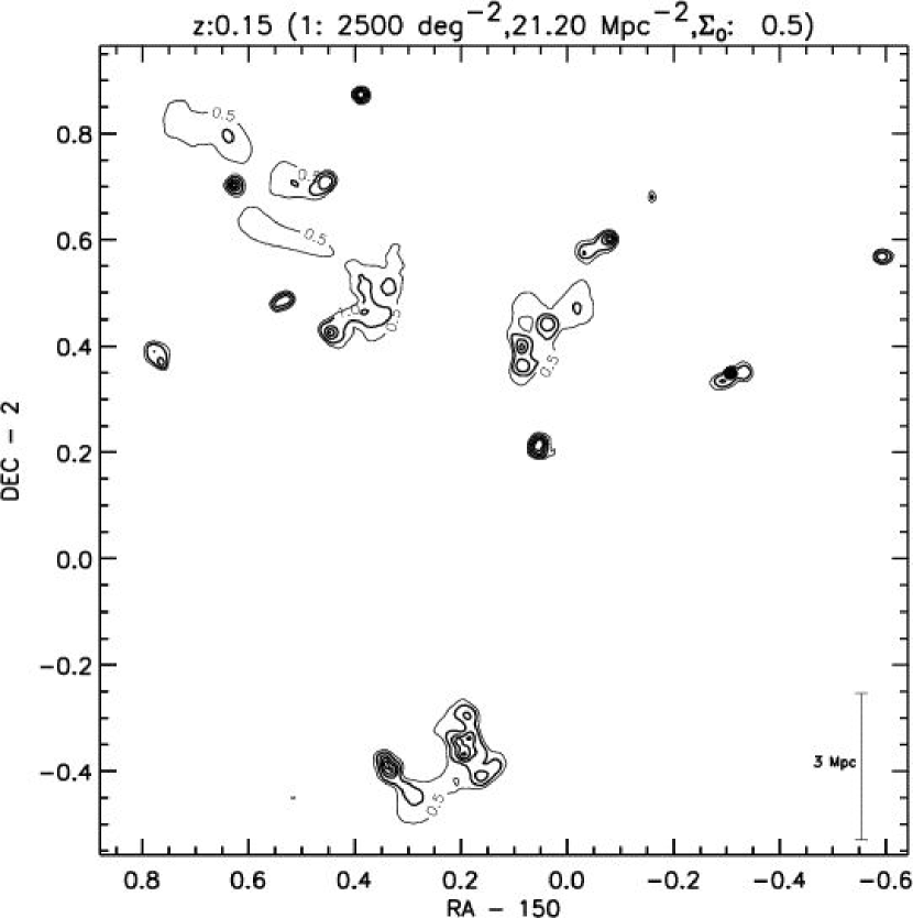
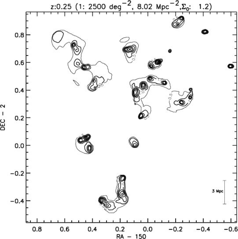
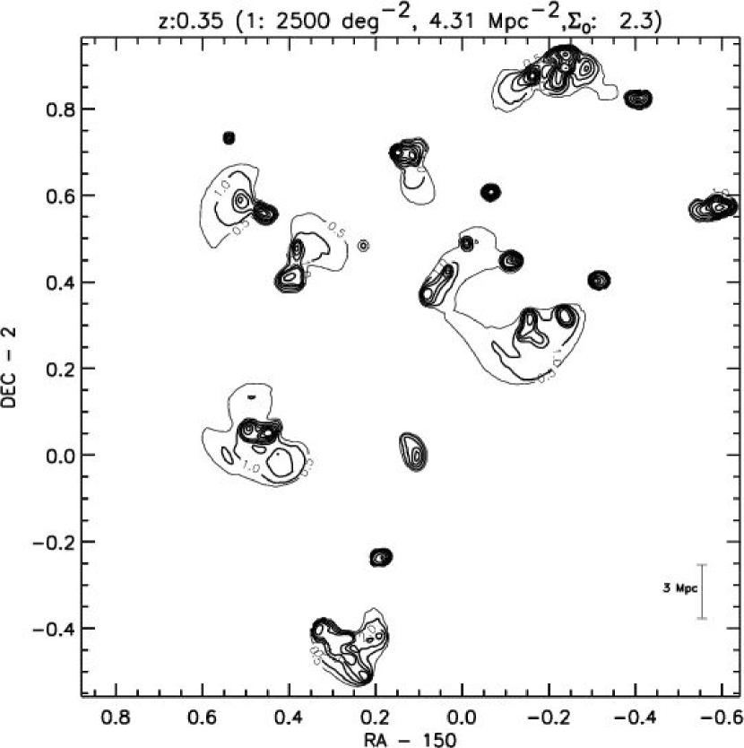
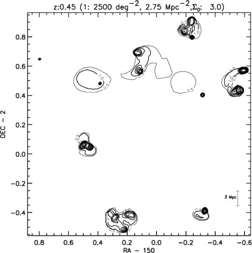
Figure 3: The surface-density of galaxies (with background subtracted out) computed using the adaptive smoothing algorithm described in Appendix A is shown for slices at different redshifts. For z $\leq 1.05$, the width of the redshift slice is $\Delta z=0.1$; for the last three plots with z $\geq 1.3$, we use $\Delta z=0.25$. On each plot, the legend at the top gives the surface density (galaxies per deg^-2 and per Mpc^-2) corresponding to 1 contour unit. The number of contour units corresponding to the background surface density ($\Sigma_{0}=B_{0}$) is also given. The scale bar indicates the size in co-moving Mpc. At higher z, we show only those redshifts with possibly significant structures.

The galaxy surface-density derived using the procedure described above and in Appendix A is shown in Figure 3 for redshift slices with $\Delta z$ = 0.1, spaced by $\Delta z$ = 0.1 for the Low-z sample of galaxies. In the last two panels of Figure 3 we show two of the higher redshift slices with $\Delta z$ = 0.25. We leave further analysis of the high redshift galaxies to a later paper since deeper near infrared and Spitzer IRAC imaging (Sanders, 2006) is required for higher accuracy photometric redshifts.

The surface-density plots show a large number of very significant large features – especially at z = 0.35, 0.75 and 0.85. And at every redshift numerous small groupings of galaxies are seen. There is a definite trend towards increasing complexity of structure (clumpiness) at higher z. This is to be expected since structures at high z (earlier epochs) are dynamically younger and expected to be less relaxed.

3.1 Structure Identification

From the derived surface density in the 3-D cube ($\alpha$, $\delta$ and z), we define preliminary LSS starting from $>10\sigma$ peaks, finding all connected pixels above the $1\sigma$ noise. Using an algorithm developed by Williams et al. (1994), approximately 140 local maxima are identified and their connected pixels catalogued. When multiple local maxima are found in proximity, the neighboring pixels are associated with the nearest local peak – this can result in subdivision of structures which have multiple peaks (real or noise). The maps of the 140 preliminary structures are therefore checked for possible recombination into composite structures. The decision to recombine was based on : whether the individual components were touching in 3-d space; their borders meshed; and their proximity in the 3-d space was unlikely by chance. This is somewhat subjective but a more physically justified recombination would require spectroscopic redshifts with accuracy similar to the virial velocities of the groups. This will become possible with the COSMOS spectroscopic surveys (Lilly, 2006; Impey, 2006).

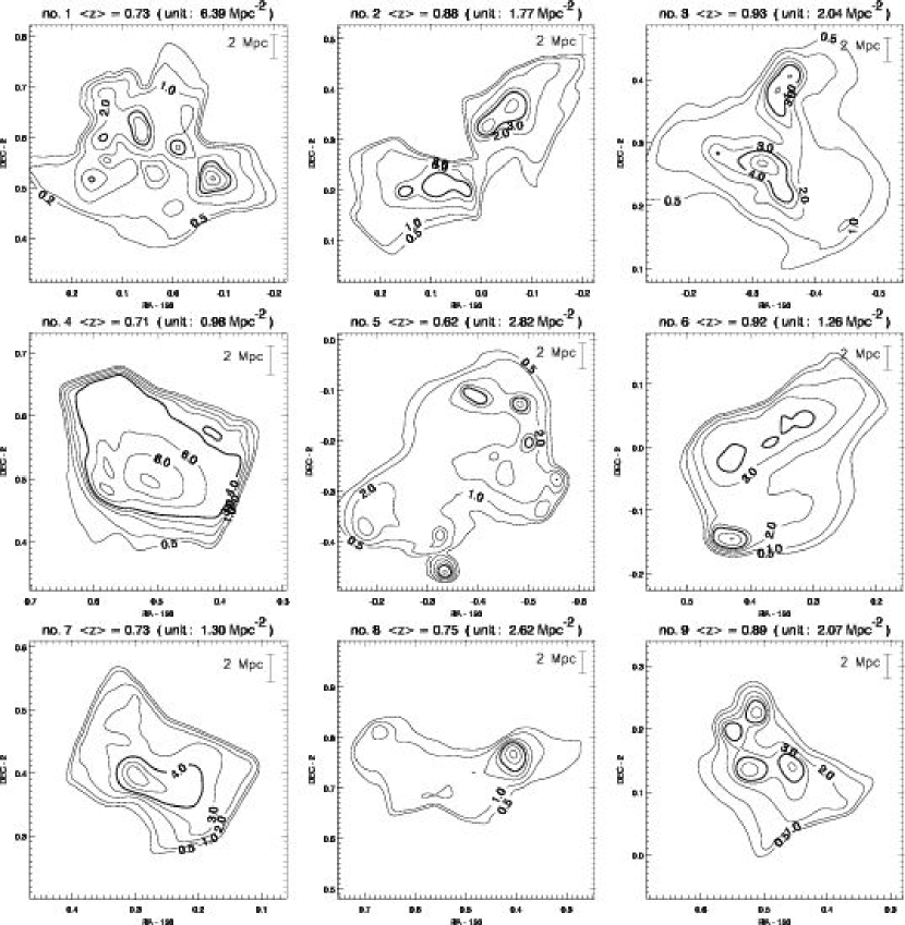
Figure 4: The surface-density of galaxies in each structure found in the adaptive smoothing procedure. The galaxy densities are integrated in redshift over all connected 3-D pixels for each structure. A scale bar on each plot indicates 2 Mpc (comoving). The top legend gives the surface-density of galaxies corresponding to 1 contour unit and the mean redshift $<z>$ of all galaxies within each structure is given.

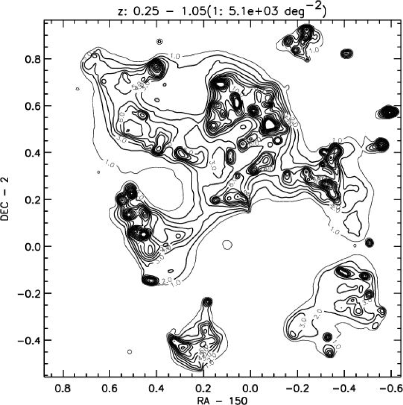
Figure 5: The galaxy overdensities derived from the adaptive smoothing results, integrated in z from z = 0.25 to 1.05. The contour units are $5.1\times 10^{3}$ galaxies deg^-2 and the contours are at 1,2,3,4,5,6,7,8,10,12,14,16,18,20,22 and 24 units.

Forty-two recombined, independent LSS were found from the procedure described above (i.e. identification of all local maxima and the subsequent recombination). The surface density of each structure, integrated in the z-dimension, is shown in Figure 4. Many of the most populated structures show complex structure with multiple peaks in $\alpha$ and $\delta$. The structures are ordered in terms of decreasing number of 3-D pixels so the most complex and massive structures are those with lowest LSS number. In Table 3 measurements for the structures are tabulated, including the location of peak density $\alpha$ and $\delta$, centroid redshift, sizes, number of galaxies and mass. Figure 5 shows the projection of all LSS on to the plane of the sky, i.e. integrating in redshift; a finding chart for the LSS within the COSMOS field is provided in Figure 6. The galaxy stellar masses are obtained from the photometric redshift fit, which yields an absolute magnitude and an SED type for the galaxy from which a stellar mass-to-light ratio can be inferred (Mobasher et al., 2006). An important consideration in measuring the structure parameters is possible contamination from the background galaxy population. This contamination is estimated from the mean surface-density in each redshift slice. Then for each galaxy, seen in projection within the area of a given LSS, the probability that it is in fact associated with the structure is given by the ratio $\Sigma_{LSS}/(\Sigma_{LSS}+\Sigma_{background})$. In calculating the cluster mass, the mass of each galaxy within it is multiplied by this local probability. Thus, the derived masses are corrected for foreground/background contamination. In the first column of Table 3, we list (in parenthesis) the ID numbers of possibly associated X-ray clusters from Finoguenov et al. (2006). The surface densities at the cores of these structures are similar to those seen in the Rich Cluster and Subaru/XMM Deep surveys ($\Sigma\sim 10--20$ Mpc^-2; O’Hely et al., 1998; Pimbblet et al., 2006; Kodama et al., 2004) but their extents at lower density go out to $>10$ Mpc. Spectroscopic redshifts from zCOSMOS (Lilly, 2006) will be needed to confirm the coherence of these more extended structures.

3.2 Radial Profiles : Clusters vs. Structures

Without spectroscopic redshifts it is impossible to determine which structures are in fact gravitationally bound. However, the spatial distributions of galaxies within the structures suggest that many of the LSS are ’relaxed’ clusters. In Figure 7, we plot the azimuthally averaged projected radial distribution of galaxies in each structure. For each LSS, radii were calculated from the position of peak number density. In several of the structures with significant secondary peaks the radial structure is not monotonically decreasing (e.g. # 10, 13 and 18). Since the largest, most complex structures have the lowest LSS numbers, these are most likely large-scale structures with multiple clusters (LSS # 1 – 8). All of these are at the higher redshifts; this is due to the greater volume sampled at z $>0.5$. They may eventually relax to form a centrally-concentrated cluster. Conversely, LSS # 30 – 42 all appear fairly symmetric in their radial distributions and with size 1 – 2 Mpc, similar to those of present day galaxy groups ($\lesssim 20$ members) or small clusters.

Most of the structures can be fit by a power law surface density of roughly $r^{-1}$, within the central few Mpc, implying that the physical density is $\sim r^{-2}$ – similar to what is usually found for local clusters such as Perseus. There are however some LSS where the density dependence steepens in the central regions; this could reflect the presence of an unrelaxed, outer ‘infall’ region. A better understanding of the nature of these density profiles and their variations will require better kinematics from spectroscopic redshifts.

3.3 Richness

The last column of Table 3 provides an estimate of the Richness of the structures using a measure similar to that used for galaxy clusters (Abell, 1958). For each structure, the central surface density of galaxies at R $\leq 1$ Mpc is listed with the background number counts subtracted off. Radius is measured from the location of peak surface density as in Figure 7. We first find the 3rd brightest (M3_V) cluster galaxy and then count all galaxies brighter than M3_V + 2 mag. (M3_V is always brighter than -20 so this procedure is not conflicting with the cutoff in Equation 1b.) The standard procedure for local clusters employs R $\leq 1.5$ Mpc, but Postman et al. (1996) find that for a typical cluster profile N($R<1$ Mpc) / N($R<1.5$ Mpc) $\simeq 0.72\pm 0.05$ , so the estimates given in Table 3 can be scaled up by approximately 1.39 to make them comparable to the standard Abell Richness criteria. The distribution of Richness parameters is shown in the right panel of Figure 8. Most of the cores of COSMOS LSS fall in Richness classes 1–3.

3.4 Structure and Cluster Masses

Figure 8 shows the distribution of photometrically derived stellar masses (Mobasher et al., 2006) for the LSS between $5\times 10^{11}$ and $\sim 3\times 10^{13}$ $M_{\odot}$. This distribution is clearly subject to significant Poisson and cosmic variances as discussed below (Section 3.5). The observed distribution increases toward low mass, but there are 4 with masses exceeding 10¹³ $M_{\odot}$. On the high mass end of the dark matter halo mass spectrum, the expected number distribution is $N(m)dm\propto m^{-1.6}$ (e.g. Benson et al. (2001)). The distribution of total stellar masses shown in Figure 8 is much less steep, but at this point the ratio of stellar to dark matter mass as a function of halo mass and z is not known.

The highest mass structure is LSS #1 with a stellar mass of 2.3$\times 10^{13}$ $M_{\odot}$; clearly, this is a super-massive structure, equivalent to that of the Coma cluster if allowance is made for a dark matter contribution. The mass in LSS #1 at z $\simeq 0.74$ is distributed over scales $\sim 10$ Mpc. In fact, the structure appears to be aggregating around a central cluster (Guzzo & Cassata, 2006; Cassata, 2006) and is therefore possibly forming a super-massive cluster like Coma. LSS #1 is also detected in the weak lensing shear analysis (Massey, 2006) and in the X-rays (Finoguenov et al., 2006). LSS # 17 seems to exhibit a very complex sub-structure as discussed in detail by (Smolčić, 2006). Within the inner $\sim 2$ Mpc of LSS # 17 there are at least $4$ X-ray luminous clusters and one X-ray quiet overdensity at the same redshift. One of the clusters hosts a wide-angle tail (WAT) radio galaxy which Smolčić (2006) discuss as a tracer for assembly of this complex cluster. They argue that the structure is in the process of formation and estimate that the mass of the final cluster, after merging of all sub-components, will be $\sim 20$% of the Coma cluster mass.

The LSS masses listed in Table 3 are for just the stellar masses as derived from the observed galaxy fluxes using a mass-to-light ratio, based on the best fit SED from the photometric redshift determination (Mobasher et al., 2006). The total masses, including non-stellar or non-luminous baryons and dark matter, are at least an order of magnitude greater – for $\Omega_{B}=0.025h^{-2}$ and $\Omega_{M}=0.3$ with H${}_{0}=70$, $\Omega_{M}/\Omega_{B}=6.1$ (Kolb & Turner, 1990). Hoekstra et al. (2006) analysed the weak-lensing maps for a sample of individual galaxies at $0.2<z<0.4$ to estimate the total virial masses and baryon fraction in the stars. They find a virial-to-stellar mass ratio $M_{vir}/{M_{*}}=20\rightarrow 40$, depending on the assumed stellar IMF and $M_{*}/M_{baryon}$ = 14% (early type galaxies) to 33% (late type galaxies) (Hoekstra et al., 2006). Similar results were found for lower redshift SDSS galaxies by Guzik & Seljak (2002) and in semi-analytic simulations (Kauffmann et al., 1999; Benítez, 2000; van den Bosch et al., 2003). Since the mass-to-light ratio (including dark matter) is found to increase as $\sim$L^1.5 at low redshift (Hoekstra et al., 2006) and presumably, the stellar baryon fraction is lower at higher redshift, we adopt $M_{vir}/{M_{*}}=50$ as a reasonable lower limit for the LSS listed in Table 3 and a more likely value might be $\sim 100$. For LSS #1 which has been analysed in detail using weak lensing (Massey, 2006), X-ray emission (Finoguenov et al., 2006) and optical (Guzzo & Cassata, 2006), the apparent ratio of total mass to stellar mass is $\sim 50$ to 100 (Guzzo & Cassata, 2006). The total masses for the LSS are therefore likely to be in the range $10^{13}$ to $\sim 3\times 10^{15}$ $M_{\odot}$.

3.5 Variances in Distributions

The mass distributions derived for the LSS are subject to both shot noise, due the small number of structures within each redshift slice, and to the cosmic variance that characterizes the mass distribution on very large scales. To estimate the resulting uncertainties in our LSS mass distributions we follow the method described by Somerville et al. (2004). We first calculate the volume and total mass ($M(vol)$) contained in each redshift slice (an area of 2.5 deg² for the photometric redshift catalog used here). The cosmic variance on this scale is given by $\sigma_{M(vol)}$ (see Figure 3-right in Somerville et al. (2004)) and the relative variance in number counts for halos of mass M_h in a redshift slice is then :

$$\sigma(M_{h},z)=(\sigma_{cosmic}^{2}+\sigma_{shot}^{2})^{1/2}$$ (2a)

$$\sigma(M_{h},z)=((b(M_{h},z)~{}\sigma_{M(vol)})^{2}+1/N_{h})^{1/2}$$ (2b)

where $b(M_{h},z)$ is the bias for the halos of mass $M_{h}$ at redshift z, calculated as in Sheth & Tormen (1999), and $N_{h}$ is the average number of halos in the slice. As explained in Somerville et al. (2004), $\sigma_{M(vol)}$ should be a slight overestimate of the true cosmic variance, since the volume in each slice is much deeper than it is wide, and thus along its $z$-axis the slice samples much larger scales where the variance is smaller.

As suggested by Mo & White (1996); Somerville et al. (2004), we can identify the appropriate mass range for halos corresponding to the LSS by integrating the halo mass function, normalized to the survey volume in the redshift slice, down to a threshold mass which yields a total number of halos matching the observed number of LSS. This assumes that the detected LSS corresponds to the most massive halos on a roughly one-to-one basis, and thus that the overall abundance of LSS indicates the characteristic mass-scale of halos with which they are associated.

In Table 4, we summarize the expected relative variances (shot, cosmic and total) in each slice for two different mass ranges of DM structures ($10^{13}$ – $10^{14}$ and $10^{14}$ – $10^{15}$ $M_{\odot}$). These variances were calculated for the cosmological parameters specified in Section 1 and with $\sigma_{8}=0.74$ (the WMAP 3-year value, Spergel et al. (2006)). Comparing the expected numbers of halos for the two mass ranges with the observed numbers of LSS, it is most reasonable to identify the observed LSS with the higher mass range halos, i.e. $10^{14}$ – $10^{15}$ $M_{\odot}$, for which the expected number is $\sim 37$. (This identification is only approximate since clearly some of the observed structures are much less massive.)

Based on the results shown in Table 4, we expect that the shot or Poisson noise and the cosmic variance are quite comparable for the mass range of the LSS sampled here at all redshifts. The total combined relative variance is expected to be in the range 0.4 to 0.6; i.e., for the very small number of very high mass structures the derived mass and number distributions will have typical uncertainties of $\sim$50% for each redshift bin.

3.6 Redshift distributions of LSS

Redshift distributions of the structures in two ranges of LSS stellar mass, M_∗ are shown in Figure 9. As discussed in Section 3.5, uncertainties due to Poisson and cosmic variance are comparable and the expected total relative variance in these number distributions is 40-60% (i.e. $\sigma_{N}/N\sim 0.5$). Also shown is the relative comoving volume (dotted line) for the redshift bins. The redshift distribution of total mass ($\Sigma M_{LSS}$) within structures with stellar masses in the range M${}_{*}=10^{12}\rightarrow 10^{13}$ $M_{\odot}$ is similar (within the expected 50% variance) to the dotted curve showing the variation of comoving volume sampled. This suggests that we are recovering structures in this mass-range without a strong redshift-dependent selection bias. The higher mass LSS (M${}_{*}>10^{13}$ $M_{\odot}$) exhibit an apparently steeper falloff at low z but this is not statistically significant given the small volume sampled. These results are consistent with a lack of dramatic evolution in the overall mass fraction for the most masssive structures out to z = 1 (a lookback time of $\sim 8$ Gyr) – as is also seen in $\Lambda$CDM simulations (e.g. Benson et al. (2001)). However, this result is certainly not strongly constraining given the large variances.

The derived mass function for the COSMOS LSS can be compared with previously derived mass distributions for galaxy clusters, mostly for clusters at lower redshift. The cumulative mass function ($n(>M)=\int_{M}^{\infty}n(m)\,dm$) is shown in Figure 10 for the 42 COSMOS LSS. The error bars are taken from the Poisson noise in each bin of width $2\times 10^{12}$$M_{\odot}$. The expected cosmic variance is comparable to the Poisson noise (see Section 3.5 and Table 4); it is not explicitly included here since it is dependent on the adopted cosmological parameters (in particular $\sigma_{8}$) and on correct identification of the associated DM halo mass range. The full error bars are likely $\sim\sqrt{(}2)\simeq 40\%$ bigger than shown when including cosmic variance. For the COSMOS sample volume we adopt 1.5 $\times 10^{7}$ Mpc³ out to z = 1.1. Also shown are the mass functions derived from optical and X-ray studies, as summarized by (Reiprich & Böhringer, 2002). The mass function for masses within the Abell radius of each cluster is M_A; masses within the regions with density exceeding 200$\rho_{c}$ and 500$\rho_{c}$ are M₂₀₀ and M₅₀₀ (where $\rho_{c}$ is the critical density for the universe, see Reiprich & Böhringer, 2002). Reiprich & Böhringer (2002) derive the total mass including the dark matter and we have scaled their masses down by a factor of 100, i.e. assuming a stellar mass fraction of 1% of the total mass (baryons plus dark matter). We have also scaled to h = 70 (used here throughout) from their h = 50.

Figure 10 shows reasonably consistent number densities (per co-moving volume) between the COSMOS LSS and the previous studies as summarized by (Reiprich & Böhringer, 2002), given the somewhat uncertain ratio of total to stellar masses (taken as 100 for Figure 10). It should be noted that the mass function within the Abell radii (labelled M_A in Figure 10) also closely approximates the mass function derived by (Bahcall & Cen, 1993). As noted in Section 3.4, Hoekstra et al. (2006) determined a value of up to $40$ for this mass ratio based on lensing measure for clusters at z = 0.2 to 0.4. The somewhat higher value, found here in order to achieve agreement in the local mass function shape, might indicate that the fraction of baryons in stars is less at the higher redshifts (z $\simeq 0.2$ to 1.1) sampled in the COSMOS LSS. Alternatively, the COSMOS LSS measurements refer to more extended, lower density structures and filaments than those sampled by Hoekstra et al. (2006) and the conversion efficiency of baryons into star is very likely dependent on environment in the context of $\Lambda$CDM models.

4 Comparison of Structures with $\Lambda$CDM Simulations

$\Lambda$CDM simulations provide quite specific and relatively confident predictions for the growth structure in the dark matter (DM) as a function of redshift, given a specified set of cosmological parameters. On the other hand, the formation and evolution of the visible galaxies within the DM structures has relied on semi-analytic models or prescriptions for star and AGN formation, stellar evolution and feedback processes. These semi-analytic models and the predicted distributions of galaxies in $\Lambda$CDM have been mostly constrained from low redshift galaxy surveys. Relatively little constraint or testing of the semi-analytics vis-a-vis the DM LSS has been done at high redshift (i.e. z $>0.2$). In this section, we compare in some detail the distributions of galaxy overdensities seen in the COSMOS field out to z = 1.1 with those predicted in simulations.

In particular, we will compare the relative volumes (or areas) occupied by observed structures of overdensity with the simulation predictions – as a function of redshift. As time progresses, the fraction of volume with high overdensity will increase and the maximum overdensity should increase at lower redshift. This measure of structure evolution enables significant comparison between the simulations and the observed universe, avoiding the azimuthal averaging which is inherent is a correlation function analysis. The structures are expected to filamentary and therefore are not circularly symmetric; they may also have multiple characteristic scales. For the same reasons, we have employed the adaptive smoothing technique developed here rather than matched filter algorithms (Postman et al., 1996; Schuecker & Boehringer, 1998) which are obviously well-adapted to the central, high density core structures but less appropriate to extended filamentary structures. Angular correlation functions for the COSMOS field are presented in McCracken (2006).

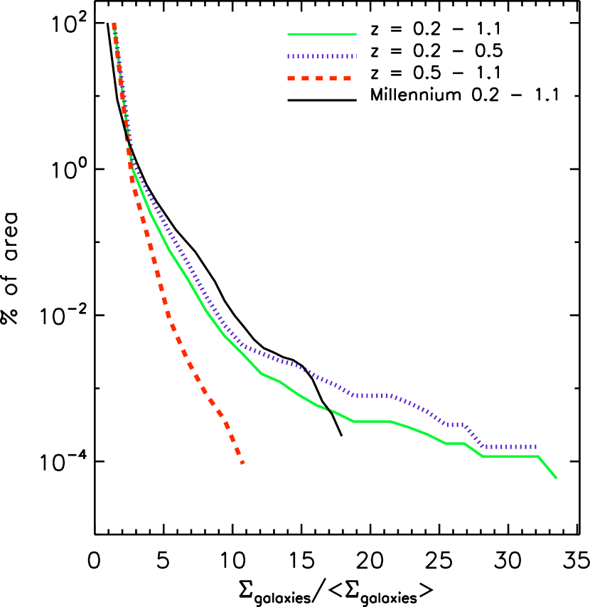
Figure 11: The cumulative fraction of survey area with surface number density $\Sigma$ relative to the average at each redshift ($<\Sigma>$) is shown for all redshifts and for low and high redshift ranges (colored curves). For comparison, the black line shows the average at z = 0.2 to 1.1 obtained from the Millennium Simulation (see text). Jackknife tests, splitting the datasets in half, showed typical variances $<20$%.

Figure 11 shows the fractional cumulative area with galaxy surface density greater than $\Sigma$/$<\Sigma>$ where $<\Sigma>$ is the average in each redshift slice. The three colored curves show overdensity filling factors for the redshift ranges 0.2 to 0.5, 0.5 to 1.1 and 0.2 to 1.1. These curves were computed from the adaptively smoothed overdensities shown in Figure 3 divided by the mean background surface density ($\Sigma_{B}$, given in the top legend for each redshift slice). The level of the background is dependent on the density of true ’field’ galaxies and on the redshift accuracy – thus in comparing with simulation predictions below, we also convolve the redshifts of galaxies in the simulation with a Gaussian of z-width matched to that of the observational photometric redshifts. Figure 11 exhibits the basic characteristic expected for structure growth as a function of redshift – higher overdensities occuring at later times (lower z) and a larger fraction of the area in overdense regions as time progresses.

A quantitative comparison can be made with the Millennium Simulation. Mock catalogs were constructed using the Virgo Consortium’s Millennium Simulation and the Galform semi-analytic model of galaxy formation. Dark matter and merger trees were extracted from the Millennium Simulation using the techniques of Helly et al. (2003) , utilizing all halos of $\geq 20$ particles. These merger trees are fed through the Galform semi-analytic model (using the parameter set of Bower et al. (2006) to populate the simulation with galaxies at all redshifts. We did not have access to proprietary lightcone data from the Millennium Simulation, so the mock catalogs were constructed taking cubes from the Millennium Simulation at z=0.3, 0.5, 0.7, 0.9 and 1.1. Regions with two sides equivalent to 1.4^∘ and one side extending 500 Mpc/h were extracted at each redshift. Galaxies were selected to have M${}_{V}<-18$ mag and 19 $<$ i $<$25. The mock based on the Millennium-Virgo semi-analytic (black curve in Figure 11) is in remarkably good agreement with the mean curve determined from the observations for z = 0.2 to 1.1 (solid green line). Jackknife tests were done, splitting the data in half and the variances are typically $<20$% for most values of the overdensity – this provides a limited estimate of the uncertainties. The overall area filling factors in the observations and theory track each other within a factor of $\sim 2$. It does appear that the theoretical curve does not reach as high overdensities as the observational curve – possibly indicating a significant discrepancy on small scales. Since what is being measured in both the observed and theoretical distributions is the number counts of galaxies, not the mass distributions, the discrepancy might indicate that the simulations have too much merging in the denser regions.

5 Correlation of Galaxy SED and Luminosity with Structure Location

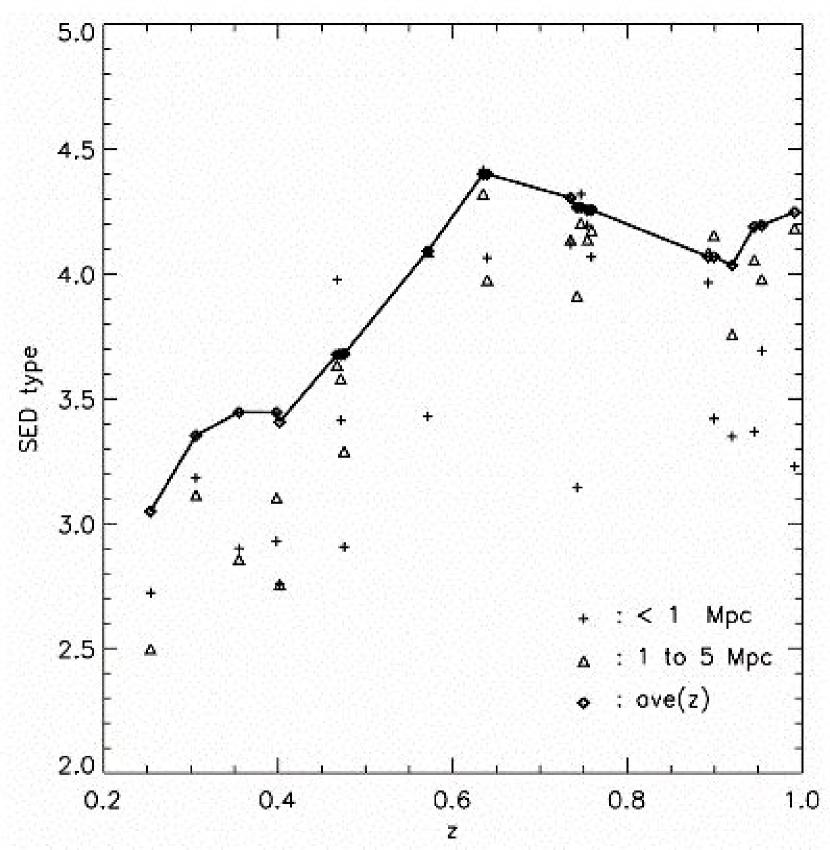
Figure 12: For each structure, the mean SED types of galaxies at projected R $<1$Mpc and R = 1 to 5 Mpc are compared (solid line) with the mean type as a function of z (in a redshift bin $\Delta z=0.2$ centered on the same redshift). One set of points is shown for each of the structures plotted at the mean redshift of each structure. Note the very pronounced trend for the central Mpc in the structures to have earlier mean SED type (low type) for the galaxies.

A number of recent investigations have found early-type galaxies more strongly clustered than the later types (Le Fèvre et al., 2005; Meneux et al., 2006; Coil et al., 2006; Cooper et al., 2006) at z = 0.5 to 2. Variation of galaxy SEDs as a function of both redshift and structure location is dramatically shown in Figure 12. Here we plot the mean SED of galaxies as a function of z (with no selection for structures or the field) and the mean for galaxies within R $\leq 1$ Mpc and R $=1$ – 5 Mpc from the center of each structure. This is on a scale with six types ranging from 1 for an E/S0 galaxy SED to 6 for a starburst galaxy (Mobasher et al., 2006). Figure 12 demonstrates dramatically, and in every case that the interior of the structures are populated with galaxies having a mean SED type lower by $\sim$0.5 – 1 compared to the average SED type at the same redshift. Butcher & Oemler (1984) first showed the trend for an increasing fraction of blue galaxies within clusters out to z = 0.5 and the trend for earlier morphological types in the highest density regions is well known as the T - $\Sigma$ relation at z $<0.5~{}$(Dressler et al., 1997). The sample shown here for the COSMOS survey is the most extensive and covers a large range of redshift ($0.1<z<1.1$) using the same technique. An analysis of galaxy morphology and environmental density in the COSMOS field is presented by Capak et al. (2006). Their results are consistent with those shown here. Figure 12 also shows a systematic gradient in the mean SED for the field galaxies – about +0.5 to later types from z =0.2 to 1.

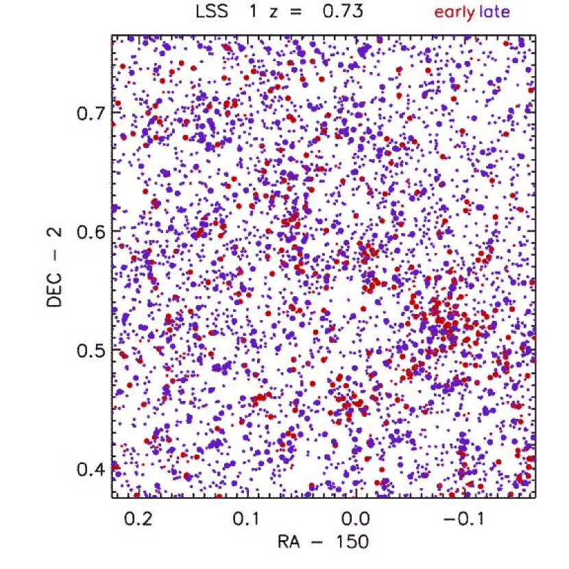
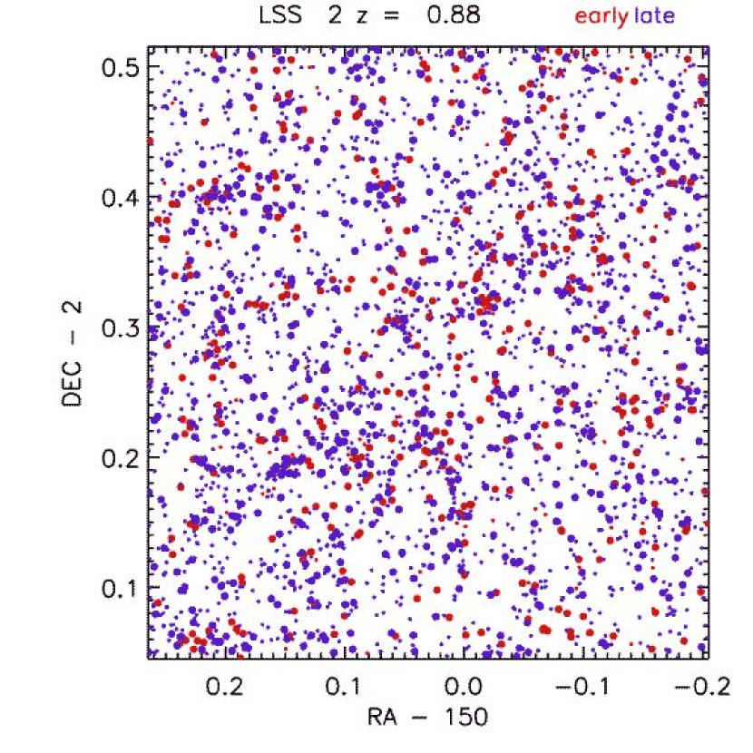
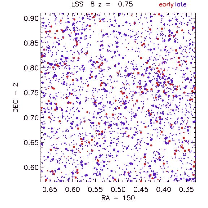
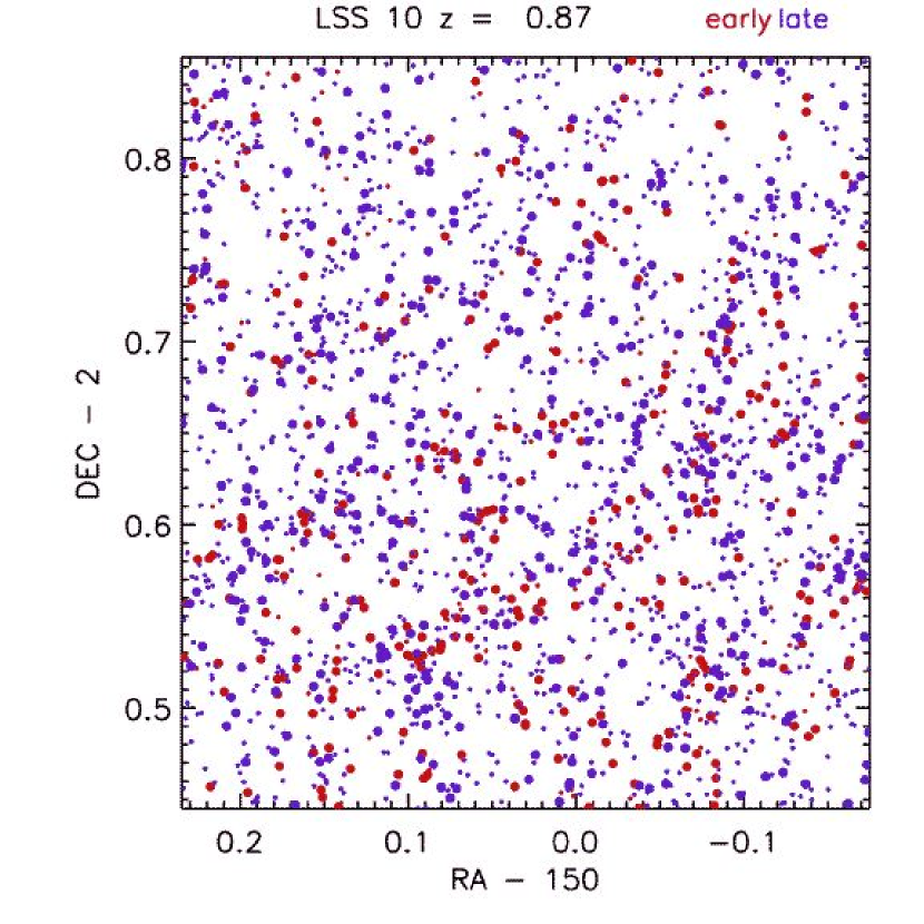
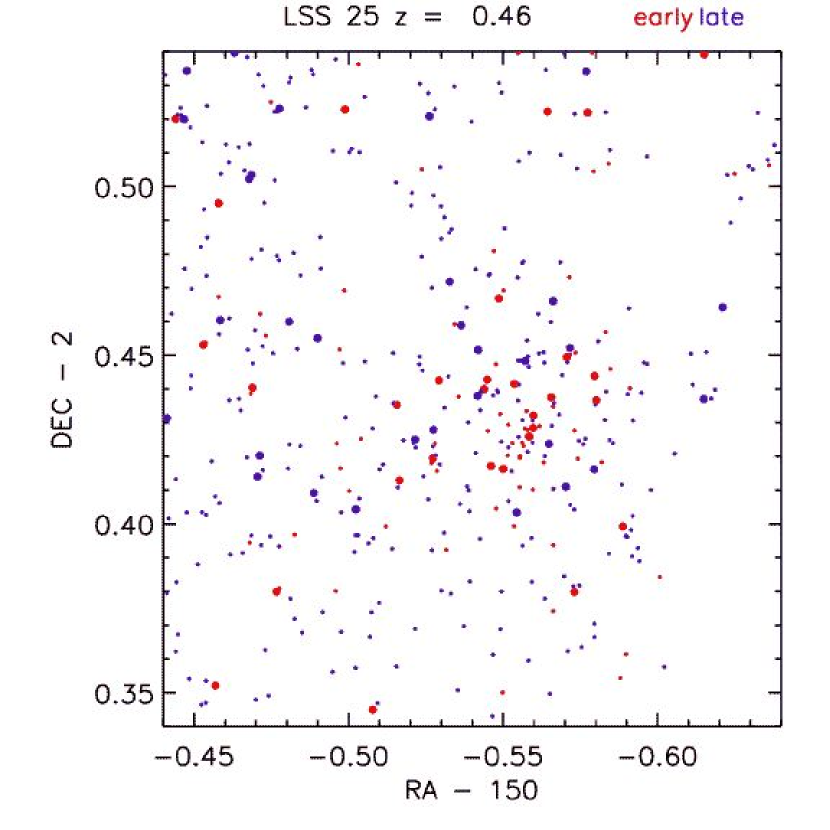
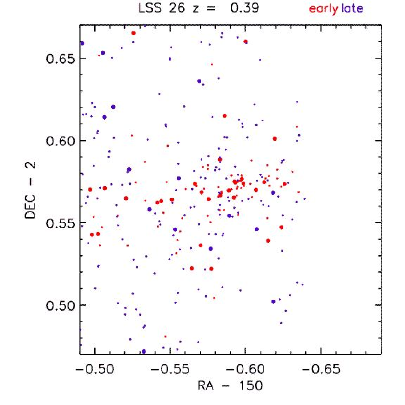
Figure 13: Galaxy distributions over the areas of 6 representative LSS (ranging from the most massive to a quite low mass structure). The red points indicate early type (SED $<2.5$) and the blue point later types. The larger dots are galaxies with M${}_{V}<-21$ mag. The galaxy points plotted in the figures have their redshifts within the $\Delta z$ range given in Table 3 for each structure. The blank areas are either at the edge of the field or where stellar masking occurs.

Figure 13 shows the fields surrounding a sample of six of the LSS (#1, 2, 8, 10, 25 and 26) with the galaxies shown in color depending on their SED type determined in the photometric redshift fit. (Galaxies within the $\Delta z$ range given in Table 3 are plotted for each structure.) These figures show the enhancements in galaxy density associated with the LSS; they also indicate the level of background contamination which any identification procedure must deal with. However, the most interesting feature easily seen in Figure 13 is the preference of the early SED-type galaxies for the denser LSS. It is important to recall that the sample selection used to identify the structures was involved all galaxy types, not just red galaxies.

6 Evolution of Galaxy Properties with Environmental Density and Redshift

The dependence of galaxy properties on redshift and environment is one of the central themes of current cosmological evolution studies (Le Fèvre et al., 2005; Gerke et al., 2005; Meneux et al., 2006; Cooper et al., 2006; Coil et al., 2006, e.g.). Here we use the overdensities derived as a function of the pseudo-3d space ($\alpha,\delta$ and z – Section 3 and Figures 3) and galaxy properties (SED type, mass, luminosity and star formation rate – SFR) derived from broadband photometry to investigate the environmental influences. Use of the density cube precludes the need to identify and delineate specific LSS (Section 5).

Our environmental densities were derived from the surface density of all galaxies (above specified mass or luminosity cuts) – the densities were not derived from clusters of color selected galaxies – thus the analysis below is presumably unbiased and without a priori correlations of environment and galaxy properties.

6.1 Environmental Density

To characterize the local environment of each galaxy, we use a ’relative density’ measure, $\rho_{rel}$ defined as

$$\rho(\alpha,\delta,z)_{rel}=\frac{\Sigma(\alpha,\delta,z)}{\overline{\Sigma}(z)}$$ (3)

where $\Sigma(\alpha,\delta,z)$ is the overdensity for each redshift slice as shown in Figures 3 and $\overline{\Sigma}(z)$ is the mean of this overdensity at each redshift. The mean value of the overdensity is used for normalization to enable comparison of widely separated redshift slices with $\Delta z=0.1$ which have somewhat different surface densities and overdensities of galaxies due to varying line-of-sight depths and comoving volumes. (The relative densities $\rho$ may be translated back to $\Sigma$ (Mpc^-2 per 0.1 in z) using $\overline{\Sigma}(z)$ = 1.2, 0.52, 0.29, 0.17, 0.14, 0.19, 0.18, 0.15, 0.13 and 0.06 for z = 0.15 to 1.05, sampled every 0.1 in z.) For each galaxy (Section 2.1), the environmental density was obtained from the pseudo 3-d cube using its $\alpha$, $\delta$ and best fit photometric redshift.

6.2 Sample Selection and Completeness

It is of course vital that the sample selection function (see Sections 2.1 & 2.2) not introduce biases as a function of redshift which masquerade as changes in the galaxy properties. We make use of two alternative samples with : #1) a mass cutoff of $M_{*}>3\times 10^{9}$ $M_{\odot}$ (82,274 galaxies)  and alternatively, #2) a luminosity cutoff with $M_{V}<-19$ mag (101,018 galaxies). Figures 2 show the observed distributions of $M_{V}$ and $M_{*}$ as a function of z. As discussed in Section 2.2, there is little change in the mass function at $z<1$ and therefore most of the variations in the mass function at M $<5\times 10^{9}$ $M_{\odot}$  are likely the result of incompleteness at $z>0.7$ (see Figure 2, right panel). Borch et al. (2006) found a possible doubling of the integrated mass function of galaxies from z = 1 down to 0.2 (in the COMBO-17 survey). We take this as an upper limit since the sample used here shows no significant variation aside from the aforementioned incompleteness (see Figure 2-right). Similarly, the selection on $M_{V}$ is chosen to be close to the limit at which completeness starts to become an issue (see Figure 2-left).

We develop the two samples in parallel since one cannot assume a priori that the galactic masses and/or luminosities are invariant from z = 1 to 0. For example, one expects the luminosity of each galaxy to vary at z $<$1 (even in the absence of further star formation or merging) due to dimming as the stellar population ages. For this reason, adoption of a fixed M_V cut would yield a sample with larger surface density at z =1 than at z =0.2. The fixed mass-cut sample most likely comes closest to generating equivalent galaxy samples at z $<1.1$; however, at higher redshifts, it is likely the masses will be changing more rapidly. A later paper will explore various evolution scenarios for the luminosity-slected sample.

More conservative higher mass and luminosity cutoffs would of course yield greater completeness at high z. On the other hand, since the various basic galaxy types have quite different masses and luminosities, this would compromise one’s ability to probe evolution between types. Specifically, a very high mass cutoff (e.g. M $>$few$\times 10^{10}$ $M_{\odot}$) would largely limit the samples to just the most massive E’s and spirals and under-represent the lower mass, late type systems which have significant star formation activity. This would severely compromise the dynamic range that could be investigated vis-a-vis the transformation from late to early type galaxies.

The distribution of $\rho$ for the sample of galaxies was also examined to select a lower cutoff in density for the analysis. This was required since very low overdensities, compared to the mean background, are not quantitatively meaningful – in areas where the adaptive smoothing detects no significant overdensity exceeding 3$\sigma$ (see Appendix A), it smoothes the surface density down to a value detemined by the largest spatial-smoothing width. The adopted density cutoff reduced the final samples to 10,382 and 12,523 galaxies for samples #1 and 2, respectively. (The lowest overdensity to which one may carry this analysis is determined by the background counts of galaxies at each redshift. This is, in turn, largely a function of the photometric redshift accuracy. Higher accuracy photometric redshifts will enable extension of this investigation to lower density and the field.)

6.3 Galaxy Properties : Mass (M_∗), SED type, Early-Type Fraction, M_V, SFR and $\tau_{SF}$

Galaxy SED types and rest-frame luminosities (M_V) are by-products of the photometric redshift fitting. Their masses were derived using the intrinsic SED to estimate the mass-to-light ratio together with the absolute V magnitude obtained from the observed fluxes (Mobasher et al., 2006). The SED types range from 1 to 6 with : 1 = E, 2 = Sa/Sb, 3 = Sc, 4 = Im, 5,6 = two starburst populations (defined by Kinney et al., 1996). The early-type galaxy fraction was calculated, taking all with SED type $<1.9$ to be ’early-type’. For each galaxy, the SFR was estimated from the intrinsic SED and observed fluxes, extrapolated into the UV. (As with the mass estimates, the SFRs have been aperture-corrected using the auto-magnitude parameter from SEXTRACTOR.) We use the SFR estimated from the extinction-corrected, rest-frame $\lambda=$1500Å continuum (Mobasher, 2006).

We also calculate the ratio of the galaxy mass to the SFR, yielding a characteristic timescale to form the existing galactic mass of stars at the currently observed SFR (specifically, $\tau_{SF}=M_{*}/SFR$). For a starburst $\tau_{SF}$ will be significantly less than the Hubble time at the observed redshift whereas a galaxy for which the current star formation is relatively low, compared to that in the past, will have a long $\tau_{SF}$. $\tau_{SF}$ is equal to the inverse of the specific SFR per unit stellar mass of the galaxy, sometimes called the ’star formation efficiency’ (SFE).

The galaxy samples were binned using 4 equal z bins of width $\Delta z=0.23$ between z = 0.2 and 1.1 and 4 logarithmically spaced bins in density $\rho$ from 8 to 215. For the adopted cosmology, the redshift bins are centered at lookback times of $\sim$ 3.5, 5.3, 6.6, and 7.7 Gyr. Within each bin, the median values of each galactic property were determined. The median was used rather than the mean since it is less susceptible to a few extreme values and hence the uncertainty in the median estimates can be small even for samples with a large intrinsic dispersion. To estimate the uncertainties in the median values, Monte Carlo simulations were done on the observed distributions, adding randomly sampled uncertainties from a normal distribution. We adopted uncertainties (1$\sigma$) in each of the bolometric quantities (M_∗, M_V and SFR) of a factor of 2 from their nominal values for each galaxy; for the SED type, we assume an uncertainty of $\pm 1$ for the type. (The factor of 2 uncertainty is an approximation to allow for uncertainties in photometric calibrations and the SED fitting.) The median was measured for each of 500 simulations, and the dispersion of the median distribution was taken as the uncertainty in the median for the observed sample.

6.4 Galaxy Evolution with Redshift and Density

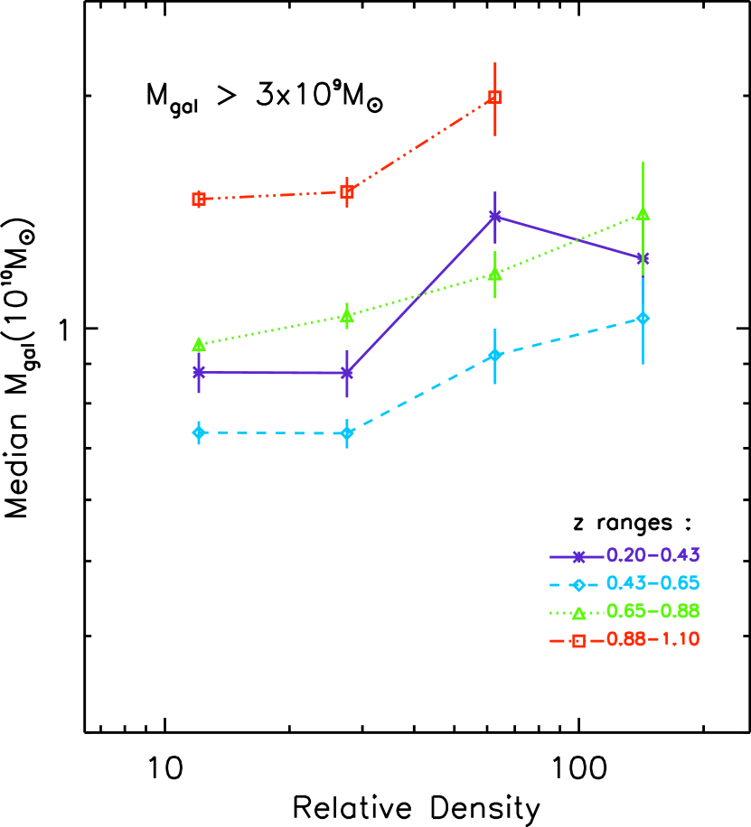
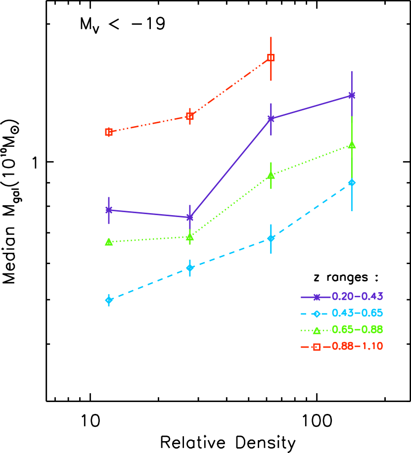
Figure 14: The median stellar mass (M_∗) is shown for galaxies binned in redshift (the curves) as a function of environmental density. Two samples are shown : M${}_{V}<-19$ mag (left panel) and M${}_{*}>3\times 10^{9}$$M_{\odot}$(right panel). (The densities have been normalized separately at each redshift for these plots (Equation 3); however, above z $\sim 0.25$ the normalizations are similar and a relative density of 10 corresponds to a surface densities $\sim 100$ Mpc^-2 – see text.)

In Figures 14 to 19, the median stellar mass M_∗, M_V, SED, SFR and $\tau_{SF}$ are plotted for each redshift range as a function of density. The SEDs, SFR and $\tau_{SF}$ all exhibit very significant variation as function of both redshift and density. The mass and luminosity distributions are partially affected by selection bias but only in the highest z bin.

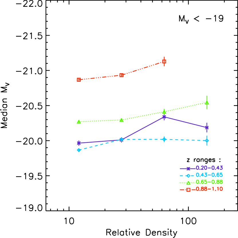
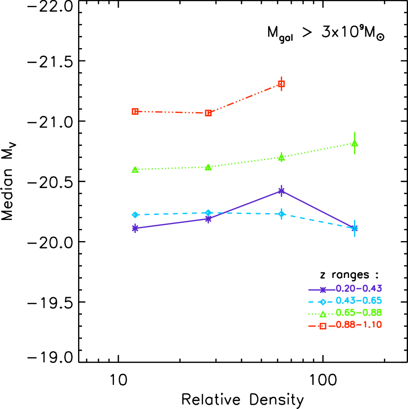
Figure 15: The median absolute magnitude (M_V) is shown for galaxies binned in redshift (the curves) as a function of environmental density. Two samples are shown : M${}_{V}<-19$ mag (left panel) and M${}_{*}>3\times 10^{9}$$M_{\odot}$(right panel).

The median mass and M_V distributions (Figures 14 and 15) and comparison of the mass- and luminosity- limited samples (left and right panels) may be used to assess the possible influence of incompleteness at the highest redshifts. The median masses show no systematic increase with z except in the z = 0.88 to 1.1 bin for which the masses appear systematically higher by a factor of 1.5 to 2 compared to lower z. This increase is very likely due to sample incompleteness or Malmquist bias since the sample is deficient in the galaxies with M_∗ $<5\times 10^{9}$ $M_{\odot}$ (see Figure 2, right panel). $M_{V}$ exhibits a somewhat larger ($\Delta M_{V}\simeq 1$ mag) increase – some of this is probably also due to incompleteness  (see Figure 2, left panel), but since it is larger than the mass shift, some of the M_V variation is likely due to actual evolution of M_V in the galaxies. Passive evolution of the stellar populations from z = 1 to 0 is $\Delta M_{V}\sim 1.2$ mag (e.g. Dahlen et al., 2005). To summarize, modest variations in the mass and luminosity medians between z = 0.8 and 1 are probably due to incompleteness; at lower redshifts, no such variations are seen and the samples are probably complete to better than $\sim 20\%$.

The median masses clearly grow with increasing density, at each redshift. This cannot be a sample selection bias since that should be constant at each redshift. The doubling of the median mass in high density environments compared to lower densities is seen at all redshifts out to z = 1; this is undoubtedly reflecting the fact that the early type SEDs also are more prevalent in the denser environments (see below) and these are often massive galaxies. Consistent with this interpretation is the fact that although M_∗ (Figure 14) exhibits dependence on $\rho$, M_V does not (Figure 15), implying that the median mass-to-light ratio is lower at high density.

6.4.1 Galaxy Spectral Type & Early-Type Fraction

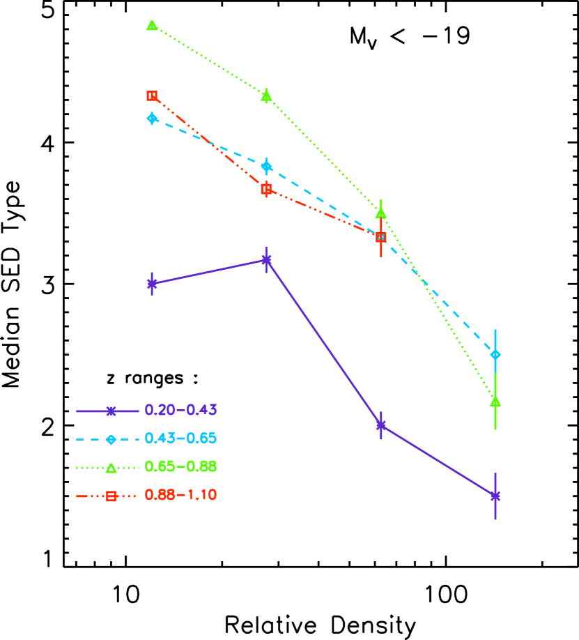
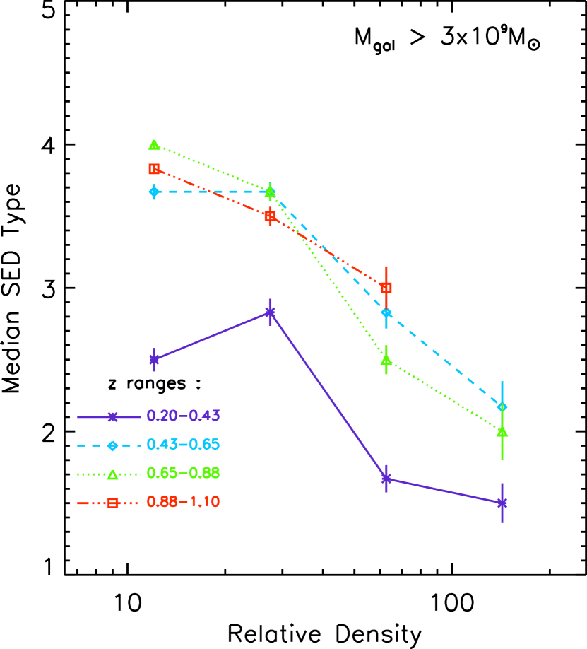
Figure 16: The median spectral type (SED) is shown for galaxies binned in redshift (the curves) as a function of environmental density. Two samples are shown : M${}_{V}<-19$ mag (left panel) and M${}_{*}>3\times 10^{9}$$M_{\odot}$(right panel).

The galaxy SED types shown in Figure 16 exhibit very significant variations with both redshift and density – in the sense that earlier type SEDs (E’s) are seen at higher density, later types in the lower density regions. And for all densities, the median galaxy type is later (i.e. bluer, star forming) at higher redshifts. The major variation with z occurs between the lowest two redshifts (from z $\sim 0.3$ to 0.5 or lookback times less than 5.3 Gyr) – all three high z bins have similar SEDs and their variations with density are the same. Numerous studies have noted the strong increase in the fraction of early type galaxies (classified by both SEDs and morphologies) in dense enviroments out to z $>1$ (e.g. Davis & Geller, 1976; Postman & Geller, 1984; Dressler et al., 1997; Kodama et al., 2004; Kauffmann et al., 2004). The results shown in Figure 16 show very clearly that similar density correlations are seen over the entire redshift range. The mean SED shifts to earlier type at lower z for both low and high density environments. The actual surface density for the breakpoint between the late and early SEDs shifts does not appear to shift more than a factor of 2 since the break occurs at approximately the same relative density $\rho$ and the density normalization from z $\sim 0.3$ to the higher z’s changes by less than a factor of 2 (see Section 6.1).

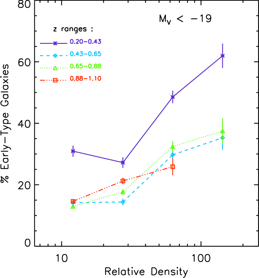
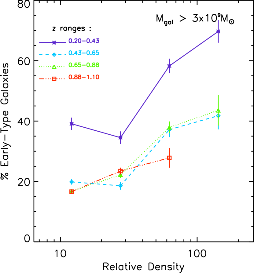
Figure 17: The median early galaxy fraction (or red galaxy fraction with type $<1.9$) is shown for galaxies binned in redshift (the curves) as a function of environmental density. Two samples are shown : M${}_{V}<-19$ mag (left panel) and M${}_{*}>3\times 10^{9}$$M_{\odot}$(right panel).

The percentage of galaxies with SED type $<1.9$ is shown in Figure 17, exhibiting variations like those in the median SED type (as it should, since they are closely related). We include the early type fraction since it is often used to characterize the galaxy populations in evolutionary studies. As with the SEDs, the major shift with z occurs beween the lowest two redshift bins, and at all redshifts an increased early-type fraction in seen above $\rho\sim 50$. Figure 17 clearly demonstrates that the galaxy-type correlation with density was clearly in place before z = 1 and we have extended this correlation to low densities, as well as the dense clusters.

6.4.2 Star Formation Rates and Timescales

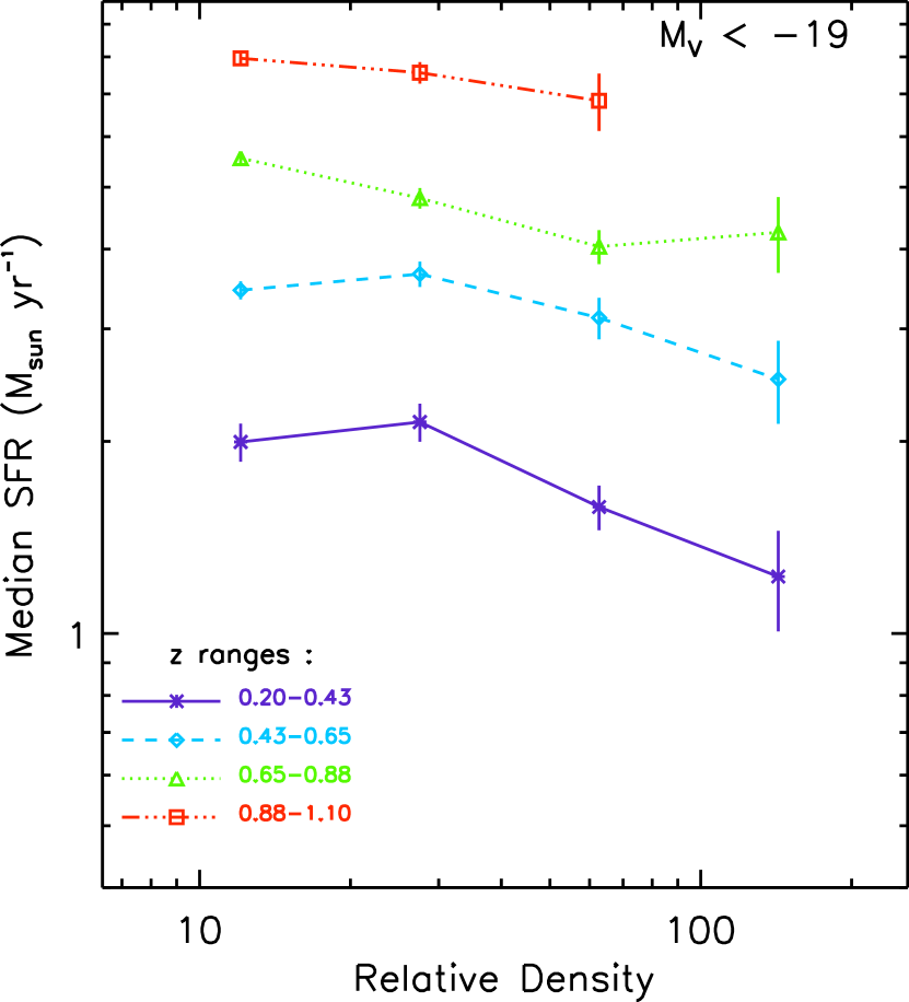
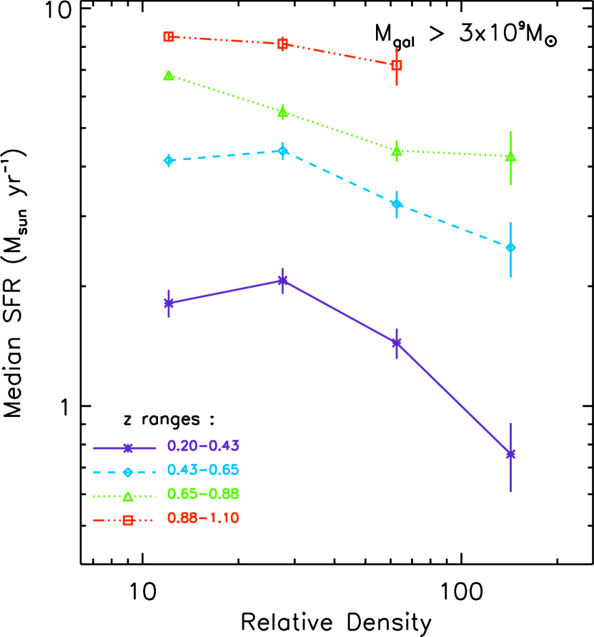
Figure 18: The median star formation rate (SFR, $M_{\odot}$yr^-1) is shown for galaxies binned in redshift (the curves) as a function of environmental density. Two samples are shown : M${}_{V}<-19$ mag (left panel) and M${}_{*}>3\times 10^{9}$$M_{\odot}$(right panel).

The median SFRs per galaxy (Figure 18) rise systematically with redshift for all densities. The overall increase by a factor of 4.5 from z = 0.3 to 1 is similar to that found in many earlier studies (e.g. see Madau et al., 1996; Hopkins, 2004; Juneau et al., 2005; Bundy et al., 2005; Bell et al., 2005; Schiminovich et al., 2005). The observed increase at higher redshift is extremely well fit by a linear dependence on lookback time over this range, $\tau_{lookback}=3.5$ to 7.7 Gyr. Figure 18 also shows evidence of a slight decrease in the median SFR at higher densities, with this decrease being steepest at low redshift (z$\sim 0.2$). The steep decline in the SFR to lower redshift is possibly due to the depletion of ISM to fuel star formation and AGN/SF feedback processes. Discriminating between these may be accomplished with future observations of the star forming gas content with the ALMA array.

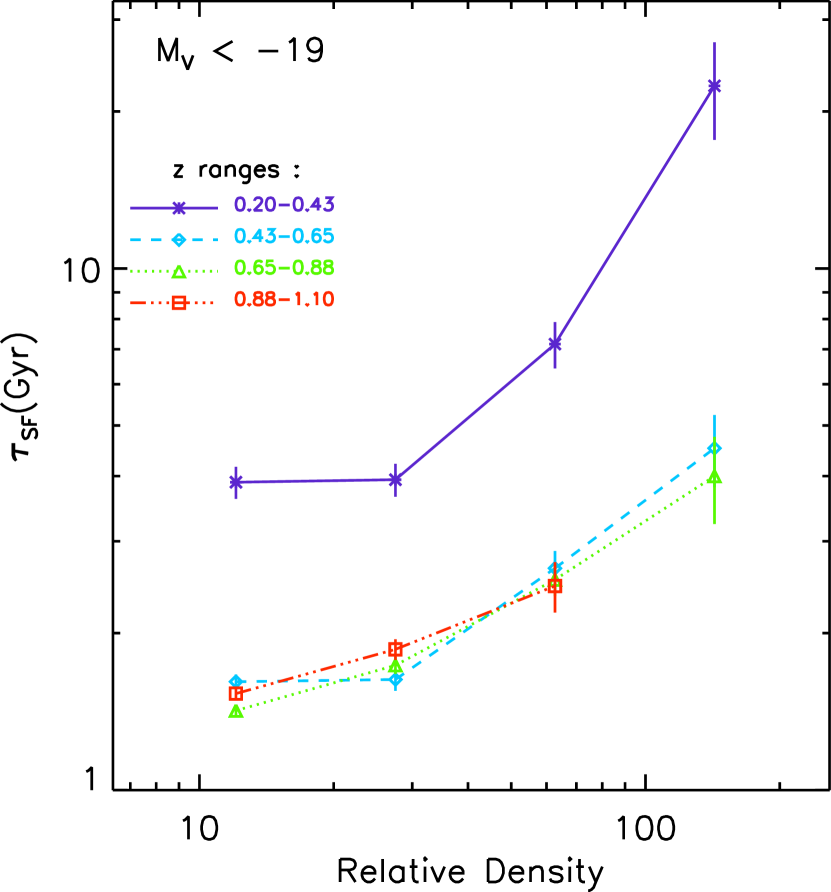
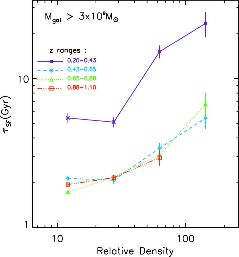
Figure 19: The median star formation timescale ($\tau_{SF}=$M_∗ / SFR) is shown for galaxies binned in redshift (the curves) as a function of environmental density. Two samples are shown : M${}_{V}<-19$ mag (left panel) and M${}_{*}>3\times 10^{9}$$M_{\odot}$(right panel).

Normalizing the SFRs by the stellar mass of each galaxy, the SF timescale ($\tau_{SF}$, Figure 19) shows much stronger density correlation than the SFR. At all densities, the SF timescale is a factor of 2 – 3 shorter in all three high redshift bins compared with z = 0.2 to 0.43. And a factor of 4 – 5 increase in the SF timescale occurs between the low and high density environments at all redshifts with the strongest density dependence occurring at the lowest redshift. These results imply that most of the stellar mass in dense environments must have formed much earlier than z $=1$ whereas a significant amount ($\sim$25%) of the stellar mass in the low density environments must have formed at z = 1.1 to 0.4 (based on the measured SF timescales).

6.4.3 Downsizing of Star Forming Galaxies – the Maturity Parameter ($\mu$)

A number of investigations have suggested that star formation occurs earlier in the most massive galaxies and as the universe ages the star formation progresses to less and less massive systems, a phenomenon often referred to as ’downsizing’ (Cowie et al., 1996; Kodama et al., 2004; Bundy et al., 2005). However, this phenomenon can be blurred and sometimes confused with the earlier formation times for galaxies in dense clusters coupled with the high abundance of massive galaxies in clusters. Here, we attempt to separate these affects to investigate the relative formation times of high versus moderate mass galaxies as a function of both redshift and density.

For this discussion, we define a parameter which we will call the Maturity ($\mu$), equal to the ratio of the star formation timescale ($\tau_{SF}$ used above) to the cosmic time ($\tau_{cosmic}$ = the age of the universe at each galaxy’s redshift). With this definition, the Maturity is unity if the observed stellar mass could have formed at the observed star formation rate within the age of the universe (at the redshift of the galaxy). The Maturity will be $<1$ (youth) if it is forming stars at a sufficiently high rate that its mass could be produced in less than the cosmic time; the Maturity will be $>1$ (middle to old age) if its current SF rate is low and most of its stars must have been formed earlier (with $\mu$ $<$1, youth) at a star formation rate much higher than that presently measured. Obviously, initial starburst systems would have $\mu$ $<<1$ and old elliptical galaxies $\mu$ $>>1$. The Maturity, defined in this manner, will continue to increase at later cosmic epochs if the star formation rate remains low. On the other hand, if the aging galaxy undergoes a late-life starburst (mid-life crisis), it will be rejuvenated ($\mu$ $\Downarrow$). But, if the the starburst is brief and not substantial, the galaxy will return more or less to its prior state of Maturity after the starburst. (As with humans, rejuvenation may be superficial and illusory ! Our use of medians for charting the overall evolution of the galaxy populations probes the typical Maturity, thus avoiding the ’noise’ due to short starbursts. [Anthropomorphizing this galactic parameter can actually help to visualize and track the galactic changes associated with evolution of $\mu$.] (This Maturity parameter is similar but not identical to the ’Birthrate’ quantity discussed by Bell et al. (2005), but ’maturity’ more aptly connotes what this parameter characterizes. )

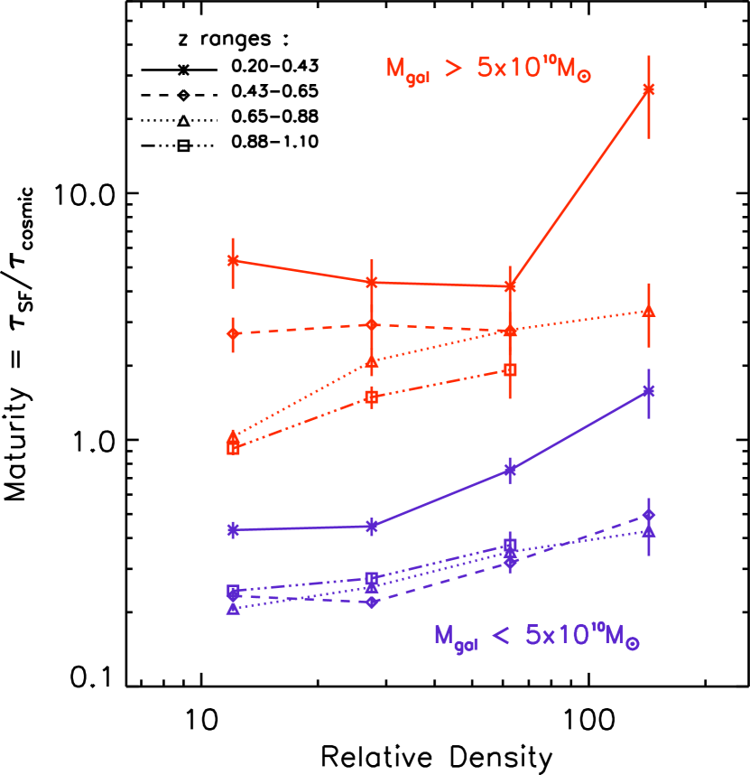
Figure 20: The median Maturity (=$\tau_{SF}/\tau_{cosmic}$) is shown for galaxies binned in redshift (the curves) as a function of environmental density. M $<1$ correspond to active, star forming galaxies and M $>1$ corresponds to galaxies which formed most of their stars at earlier epochs but see text for a more detailed discussion for interpretation of the Maturity.

In Figure 20 the Maturity is shown as a function of both redshift and density, separately for galaxies of high and low mass. The two samples were separated at M${}_{*}=5\times 10^{10}$ $M_{\odot}$. Kauffmann et al. (2004) and Kodama et al. (2004) found a ’break’ between old, red galaxies and younger, blue galaxies at a mass of $\sim 3\times 10^{10}$$M_{\odot}$ at z = 0 and 1, respectively. We have adopted a somewhat higher value in order to minimize incompleteness in the low mass sample at z $\gtrsim 1$. Bundy et al. (2005) argue that the break mass varies with redshift, rising to $\sim 10^{11}$ $M_{\odot}$ at z =1; however, we do not see such clear variation (see below). In any case, we have found by experimenting with the mass cut that a factor of 2 variation in the vale mass cut (from $5\times 10^{10}$ $M_{\odot}$) did not change the behaviors discussed below.

Figure 20 shows that at all redshifts and densities probed here, the more massive galaxies are always more mature than the lower mass galaxies. At each redshift and environmental density, the lower mass galaxies are systematically 5 – 10 times less ’mature’ than the massive galaxies. Once again, we emphasize that these are not color-differentiated galaxy samples – just mass-differentiated for which there is no a priori association with ’age’. Although, if the more massive galaxies tend to be more mature, obviously, they will appear redder.

For both the high and low mass galaxies, the median Maturity is either constant or increases with time, i.e. to lower redshift (Figure 20); it never decreases with time – as well it could if the star formation in either environment was delayed to commence at a late epoch (e.g. some dwarf galaxies). A constant Maturity implies a steady SFR over cosmic time, whereas an increasing maturity suggests diminishing SF with time. The more massive galaxies clearly must have had an early phase of rapid star formation at z $<2$ (c.f. Juneau et al., 2005) with relatively little star formation at z $<1.1$ in order to appear so mature ($\mu$ $\simeq 1$ to 2 at z $\sim 1$, Figure 20). By contrast, the lower mass galaxies exhibit fairly constant immaturity down to z $\sim 0.43$, implying that on-going, fairly constant star formation has occurred from z = 1.1 to 0.43 and very likely also at the high z. However, at the z $<0.43$ the maturity of the lower mass galaxies rises in all environments, implying a significantly decreased star formation rate for lookback times $<5$ Gyr.

Figure 20 suggests that galaxies of all masses (at z $\leq 1.1$) are more mature in the dense environments, not just the high mass galaxies! The lowest redshift bins both show $\tau_{sf}/\tau_{cosmic}$ rising quite significantly at the highest density while at the other redshifts, a factor $\sim 2$ increase in the maturity occurs between the lowest to highest densities. This clearly requires that the epoch of rapid star formation for galaxies of both high and lower mass must be earlier in the denser environments than in the field.

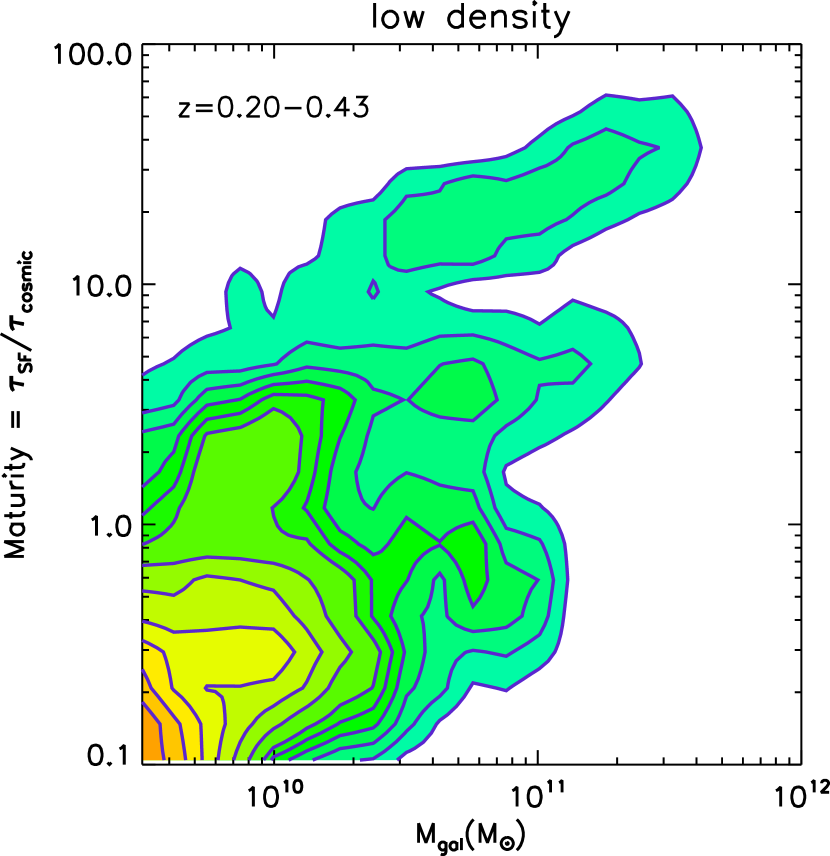
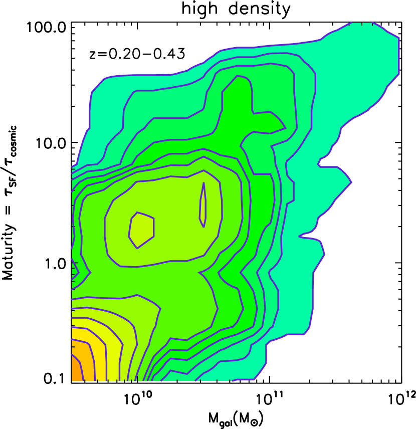
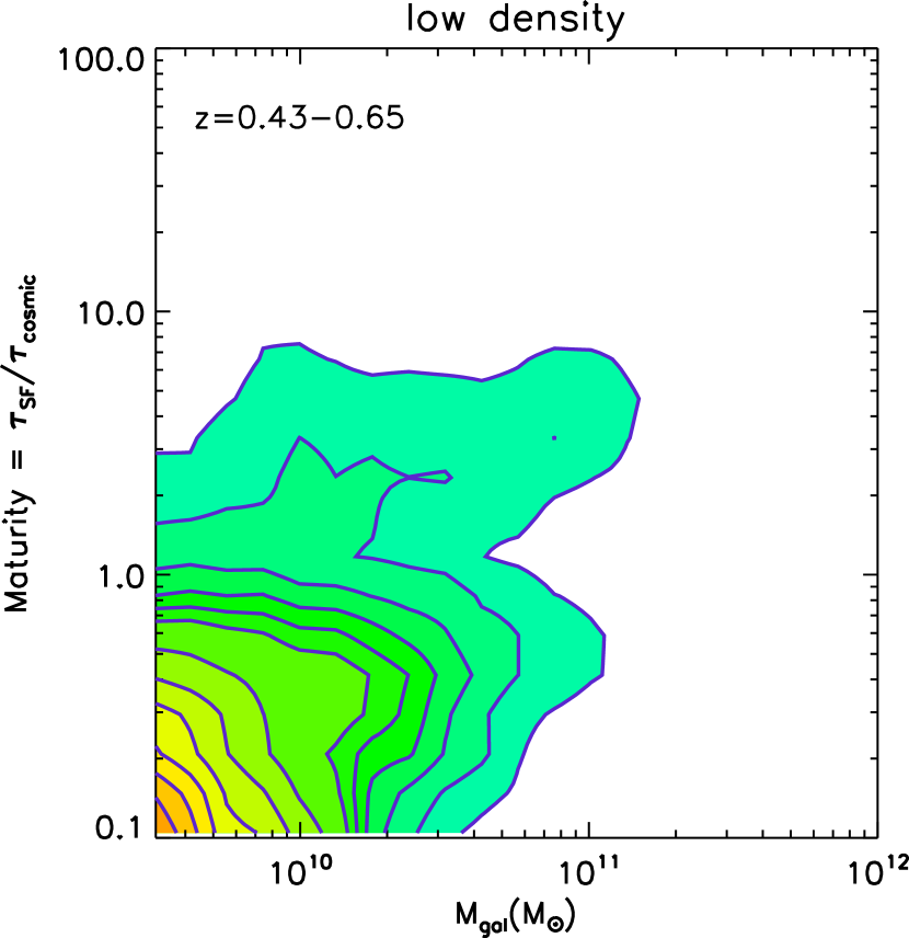
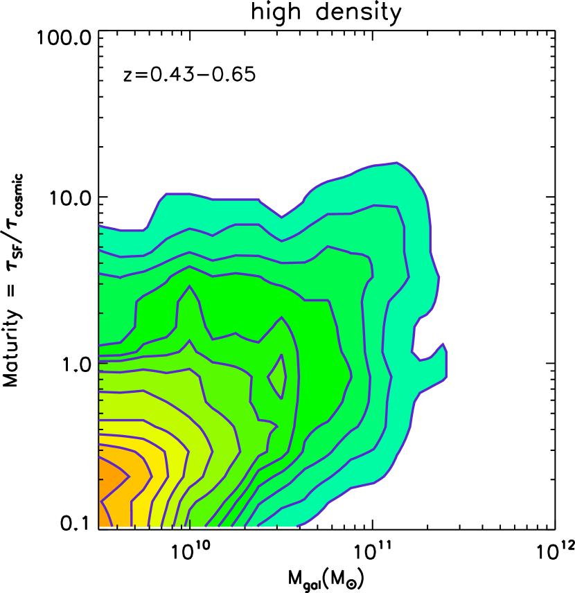
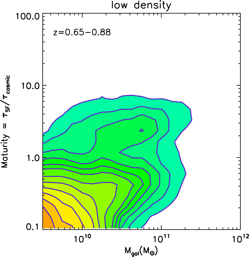
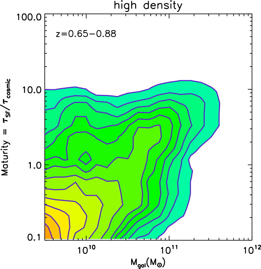
Figure 21: The Maturity ($=\tau_{SF}/\tau_{cosmic}$) is shown as a function of galactic mass for high and low density environments in three redshift bins. The cut between high and low density was taken at relative density $\rho=45$, i.e. between the middle two bins of the 4 density bins used earlier. M $<1$ correspond to active, star forming galaxies and M $>1$ corresponds to galaxies which formed most of their stars at earlier epochs but see text for a more detailed discussion for interpretation of the Maturity. Contours are normalized at 0.05, 0.1, 0.15, 0.2, 0.25, 0.3, 0.4, 0.5, 0.6, 0.7, 0.8, 0.9 times the peak.

In Figure 21 the Maturity is shown as a function of galactic mass for high and low density environments, with separate plots for each redshift. The cut between high and low density was taken at $\rho=45$, i.e. between the middle two bins of the 4 density bins used earlier. In Figure 21, the overall distribution of galaxies for all densities is shown by the colored shading while the high and low density environments are shown in the red and blue contours, respectively. The separation of the old ($\mu$$>1$) and young ( $\mu$$<1$) galaxies is seen as a bimodal distribution and their loci change systematically with redshift. Evidence of evolution in the mass separating starforming and non-starforming has been claimed by Bundy et al. (2005) and Borch et al. (2006). Bundy et al. (2005) found $M_{break}\propto(1+z)^{4}$; however, we find it difficult to identify a distinct mass which can be said to divide the mature and immature populations, since at most masses between $10^{10}$ and $10^{11}$ $M_{\odot}$ , $\mu$ can range from $<1$ to $>10$ (see Figure 21). Most of the mature galaxies occur above few$\times 10^{10}$ $M_{\odot}$, but there is no sharp cutoff at most redshifts. In fact, for the lowest redshift bin, two distinct, mature sequences can be seen at $\mu$$\sim 5$ and 20 – 30. The latter could correspond to the maturation of the $\mu$$\sim 6$ to 8 sequence seen at higher z; the former might correspond to maturation of the $\mu$$<1$ galaxies seen at earlier epochs. Possibly, the combination of these two mature sequences at low redshifts account for the apparent evolution of the break mass as discussed by Bundy et al. (2005). Future work is planned using the COSMOS GALEX UV measurement to verify this second mature sequence.

Galactic down-sizing with the most massive galaxies forming earliest is of course at variance with the expectation of the most simple hierarchical galaxy formation scenarios. However, Kaiser (1984) and later Cen & Ostriker (1993) suggested a model of biased galaxy formation with the most massive galaxies forming within the highest peaks of the initial density field, and this is a commonly accepted explanation. In the highest peaks, there is more mass available for buildup of the most massive galaxies and the rate of growth is higher where the density of sub-halos is higher (e.g. De Lucia et al., 2004). The results shown here suggest that even at relatively low environmental densities, the more massive galaxies are formed earlier than the low mass galaxies – although not as early as the massive galaxies in very dense environments. This suggests that the formation of massive galaxies occurs by two processes – one local, responsible for the early growth of massive galaxies in low density regions, the other associated with high overdensity regions where the growth occurs more rapidly and in some cases is carried to the very highest galactic masses.

7 Summary and Conclusions

The COSMOS photometric redshifts now have sufficient accuracy ($\sigma_{z}/(1+z)\simeq 0.03$) to enable identification of LSS at z = $0.1$ to 1.1. We have developed an adaptive smoothing procedure to be applied to the galaxy density distributions in photometric redshift slices with $\Delta z=0.1$ to identify LSS on scales less than 1 Mpc up to 30 Mpc with optimal signal-to-noise ratio across the range of spatial scales. This procedure has been tested with excellent results on mock redshift slices and on the dark matter particle distribution from a $\Lambda$CDM simulation (see Appendices A.2 and A.3).

The adaptive smoothing is applied to the COSMOS photometric redshift catalog with selection z $<1.1$, 19 $<$I${}_{AB}<$25 mag and M${}_{V}<-18$ mag – a sample of 150,000 galaxies. No color or SED selection is imposed, so that the defined structures are intrinsically unbiased with respect to galaxy type. From the galaxy over-densities derived from the adaptive smoothing, we have delineated 42 LSS and galaxy clusters in the pseudo 3-d space ($\alpha,\delta$,z). The surface density plots of the structures are shown in Figures 4 and 5; their measured properties are given in Table 3. Five of the most massive structures have stellar masses (determined from the galaxy photometry) of M${}_{*}>10^{13}$ $M_{\odot}$. Several have extents which can be traced over 10 Mpc (comoving). Their total masses including dark matter are likely to be 50 – 100 times greater. The Richness of the core regions of these structures is typical of Abell class 1 - 3. The derived mass function for the LSS is consistent with the total mass function for clusters derived by (Bahcall & Cen, 1993; Reiprich & Böhringer, 2002) from optical and X-ray studies.

The clusters at the center of the most massive LSS (#1) are discussed in detail by Guzzo & Cassata (2006) and Cassata (2006). The compact structures with diffuse X-ray emission, many of which are located within the LSS discussed here, are discussed by Finoguenov et al. (2006). These clusters are identified optically by wavelet analysis of the early type galaxies in the COSMOS photometric redshift catalog and from the diffuse X-ray emission. We have compared the fractional areas seen at different overdensities and find general agreement to within $\sim 50$% with the predictions of $\Lambda$CDM simulations (processed similarly) – with less than 1% of the areas of the redshift slices having overdensities exceeding 10:1. However, the observed filling factor distribution does reach higher overdensity and this may indicate that the simulations have too high an efficiency for merging in dense regions.,

We have investigated the dependence of galaxy evolution on environment using the structures defined here and the SED types taken from the photometric redshift fitting. We find that in every structure the mean galaxy SED type within the high density core of the structures is earlier than the mean SED type at the same redshift. Our study thus confirms, with a sample of 42 structures/clusters, the correlation of galaxy evolution with environmental location (e.g. Dressler et al., 1997; Smith et al., 2005; Postman et al., 2005; Cooper et al., 2006, and references cited therein)) over the full range of redshift z = 0.1 to 1. Capak et al. (2006) find a similar result using an entirely independent measure of environmental density and using galaxy morphology instead of SED type.

Extensive analysis was done to analyze the correlations of galaxy properties (SED, mass, luminosity and SFR) with redshift and enviroment. The median SED type and star formation activity varies strongly with both redshift and environmental density. The maturity of the stellar populations and the ’downsizing’ of SF in galaxies are both strongly varying with epoch and environment. Although the more massive galaxies clearly tend to have lower SFR per unit galactic mass, we question whether it is possible to define a distinct ’break mass’ separating active and inactive star-forming galaxy populations. And over the range z $<1.1$, we don’t see strong evidence of evolution in the masses of galaxies undergoing active star-formation (at the level of $<$ a factor 2).

Appendix A LSS Identification with Adaptive Smoothing

In the past, a number of algorithms or techniques have been used for automated identification and characterization of galaxy clustering, including percolation and Voronoi tesselation techniques (van de Weygaert, 1994; Ebeling & Wiedenmann, 1993; Marinoni et al., 2002; Gerke et al., 2005), wavelet analysis (Escalera & MacGillivray, 1995; Finoguenov et al., 2006) and matched filter (Postman et al., 1996; Schuecker & Boehringer, 1998). An algorithm for the identification of structures must be capable of detecting structures on multiple angular scales, and with only low order assumptions regarding the internal density profile of the structures. Techniques which search for a particular scale or assume, a priori, a density profile (or equivalently a spatial weighting function) will have highest sensitivity for structures with the specified parameters, thereby biasing a derived distribution function for the recovered structures. It is also highly desirable that the algorithm be capable of displaying compact structures simultaneously with more extended, low density structures. Presumably, within large structures there will be high density substructures which one would not want to smooth out into low spatial frequencies. Conversely, if a high density structure is fully detected at high spatial frequencies, one would not want its power to be carried out to low spatial frequencies as an extended halo. Multi-scale algorithms like wavelet and adaptive smoothing seem therefore most appropriate.

For the structure identification, we have developed an adaptive kernel smoothing algorithm, specifically tailored to have these characteristics.

A.1 Algorithm

The algorithm consists of a loop, starting at low smoothing width, going to successively larger smoothing kernels, removing power from the current 2-d residual ’image’ if it exceeds a specified signal-to-noise ratio at the current level of smoothing. The ’image’ being processed is the projected surface-density ($\Sigma$) of galaxies in a redshift slice. Starting at the initial highest resolution (n=1), we calculate the smoothed surface-density ($\Sigma_{n}$) and background surface-density (B) from

$$\Sigma_{n}=\Sigma^{\prime}_{n-1}~{}\star~{}K_{n}$$ (A1a)

$$B_{n}=(\Sigma^{\prime}_{n-1}-\Delta_{n})~{}\star~{}K_{2n}$$ (A1b)

where ’$\star$’ is the convolution operator, K_n is a 2-d smoothing kernel of width n, normalized such that its integral is unity and the Kernel K_2n used to convolve the background has twice the width, ie. 2n. The ’power available’ at resolution n is calculated as

$$\Delta_{n}=\Sigma_{n}-B_{n}$$ (A2)

Since Eq. A1b depends on A2, these equations are iterated (typically 4 times) to arrive at the ’best’ estimates of the background (without the high frequency power included) and the $\Delta_{n}$ with the most low frequency, background removed.

If $\sigma_{n}$ is the noise ’image’ at resolution n, then the signal-to-noise ratio, S($\Delta$)_n, on the delta residual-density is then

$$S(\Delta)_{n}=\frac{\Delta_{n}}{\sigma_{n}}$$ (A3)

and the signal-to-noise ratio, S($\Sigma$)_n, on the original surface-density, smoothed to resolution n, is

$$S(\Sigma)_{n}=\frac{\Sigma_{0}~{}\star~{}K_{n}}{\sigma_{n}}$$ (A4)

The power to be removed at resolution n is then given by

$$P_{n}=\left\{H\left(S(\Delta)_{n}-snr_{\delta}\right)~{}\cdot~{}H\left(S(\Sigma)_{n}-snr_{total}\right)\right\}\cdot\Delta_{n}\\$$ (A5)

where H(x) is the Heavyside function (H=0 for x $\leq$ 0, H=1 for x $>$ 0). ’snr_δ’ is an adjustable parameter specifying the minimum signal-to-noise ratio in the residual image required before power is removed at width ’n’. Similarly snr_total is a parameter specifying the minimum signal-to-noise ratio required when the original total-power surface-density is smoothed to resolution ’n’. Having these two conditions is crucial to the excellent results obtained with this procedure – allowing small values of snr_δ to be used while avoiding the retention of ’noise’ peaks. For any pixels which do not satisfy this double criteria for signal-to-noise ratio, the residual power is retained to the next level of smoothing. The residual image (with lower spatial frequency power) to be used as input on the next iteration at larger smoothing kernel (n+1) is therefore given by

$$\Sigma^{\prime}_{n}=\Sigma^{\prime}_{n-1}-P_{n}$$ (A6)

Steps A1 to A4 are repeated with successively larger values of ’n’ up to n_max.

After reaching n_max, the adaptive smoothed surface-density ($\Sigma_{final}$) is then given by

$$\Sigma_{final}=\Sigma^{\prime}_{n}+\sum_{n}P_{n}$$ (A7)

The procedure described above has the following desirable features :

1) It is conservative, i.e. the 2-d integral of the original and final surface-densities are equal.

2) Power is retained at the highest spatial frequencies and not smoothed out to lower frequency as long as its signal-to-noise ratio is sufficient (i.e. greater than the specified snr_δ).

3) High frequency power is removed first, extended haloing around high density regions is thus minimized.

4) Features seen in the final adaptively smoothed surface-density have a well-determined significance and resolution.

One caution : since the resolution is variable across the adaptively smoothed ’image’, the usual intuition that judges significance or signal-to-noise ratio by comparison with the amplitude of high-frequency noise is not reliable.

There are several parameters which are important to results of the adaptive smoothing process outlined above :

1) the signal-to-noise ratio, snr_total, to be required in the total surface-density, $\Sigma$ (smoothed to the current resolution). This parameter is set at snr_total = 3 so that virtually all features seen in the final adaptively smoothed image will be ’statistically’ significant.

2) the signal-to-noise ratio, snr_δ, specifying whether the $\Delta_{n}$ signal is removed before proceding to a lower resolution filter. This parameter should be set such that power is removed at the highest spatial frequency for which there is a ’reliable’ signal, but avoiding removal of what is essentially low-frequency power before ’its time has come’. Based on trial and error, we have adopted snr_δ =1 for the LSS identification. Although it might seem that 1 $\sigma$ would be risky, the 3 $\sigma$ condition (above) assures that most features will be significant.

3) the maximum filter width, n_max. The maximum filter width was taken at 0.33^∘, i.e. 23% of the linear size of the COSMOS field.

Two smoothing kernels were used : a boxcar and Gaussian. The boxcar was used for program development since it was faster, but all final results employ a 2-d, symmetric Gaussian filter (implemented with a Fourier transform for speed). It is well known that boxcar filters can introduce high spatial frequency edges whereas the Gaussian is better behaved in this respect.

A.2 Simulation Tests

To test the algorithm described above with conditions similar to the galaxy counts in the COSMOS photometric redshift catalog, we have simulated a single redshift slice with 10,000 galaxies. Approximately half of the galaxies were distributed within Gaussian profile structures with a distribution of peak densities and sizes. The other half of the sample galaxies were distributed randomly across the field.

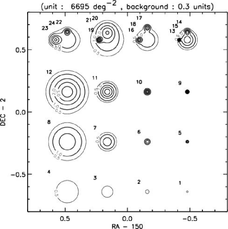
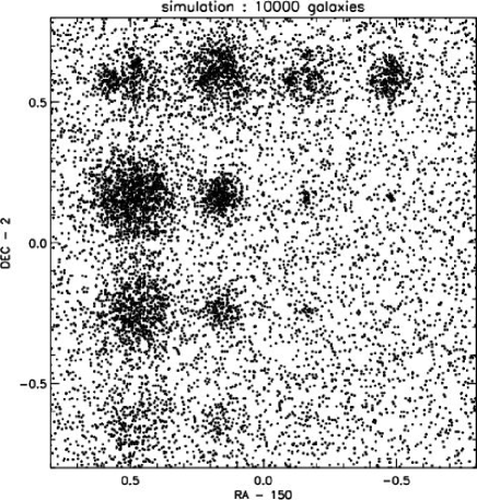
Figure 22: a) Top : The projected model densities of the clusters are shown for the parameters given in Table 5. The number to the upper left of each feature are the structure ID’s given in Table 5. The contour units are given in the top legend, along with the background $\Sigma$ in the same units. b) Bottom : The positions of 10,000 galaxies (including 5260 randomly placed galaxies) are shown for the cluster distribution in the top figure.

The parameters for the Gaussian-profile structures in the simulation are listed in Table 5. Figure 22a shows the input surface-densities profiles. For the lowest 3 rows, the simulated structures have increasing peak surface-densities toward the top and increasing in size going to the left. The top row simulates more complex structures with three internal components having varying sizes and surface densities. Figure 22b shows the simulated distribution of galaxies, consisting of 5260 galaxies randomly placed and 4740 galaxies populated with probability given by Figure 22a. It is important to realize that since the density profiles of the structures are sampled randomly, the simulation distribution, input to the adaptive smoothing algorithm, is not identical to that shown in Figure 22a, i.e. there is shot noise. Therefore, the algorithm should not be expected to return the smooth input distributions (Figure 22a) exactly.

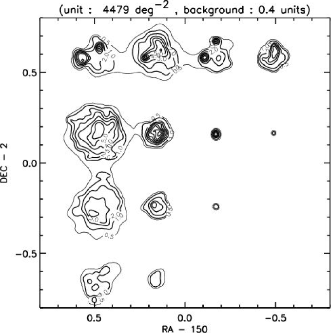
Figure 23: The density distribution recovered using the adaptive smoothing algorithm.

Figure 23 shows the surface-density recovered from the galaxy distribution shown in Figure 22b using the adaptive smoothing. In fact, the algorithm has done an excellent job of recovering all structures which were statistically significant in Figure 22b, including the top row with complex, internal structure. The three structures in the lower right of Figure 22a were not recovered but these were all sufficiently low in surface-density and/or size that their total numbers of galaxies were not statistically significant (2, 8 and 6 galaxies respectively – see Table 5). Lastly, it is worthwhile to emphasize that the algorithm did not find structures which were not in the input simulation, i.e. noise in the random galaxy population was not falsely detected using parameters for the simulation distribution (numbers of galaxies and fraction in structures) and for the detection algorithm similar to those used for the COSMOS structure detection.

A.3 Test on $\Lambda$CDM Simulations

As an additional test we have applied the adaptive smoothing procedure to one of the Virgo consortium $\Lambda$CDM simulations (Benson et al., 2001) and the more recent Millennium simulation COSMOS wedge (Springel et al., 2005; Croton et al., 2006).

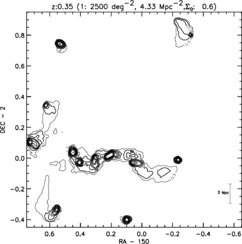
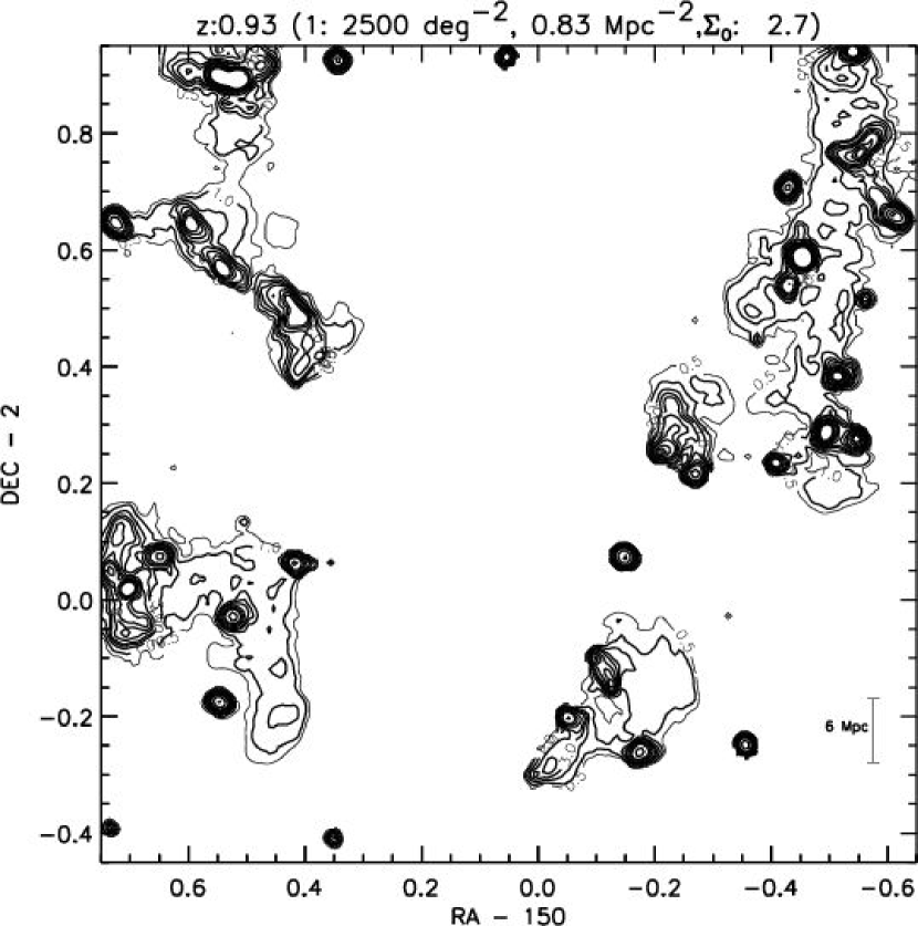
Figure 24: Application of the adaptive smoothing algorithm to the dark matter particle distribution in one of the Virgo consortium $\Lambda$CDM simulations (Benson et al., 2001). The algorithm detects virtually all significant structures seen visually in the simulation. More importantly, the characterisitcs of the detected structures (their scales and changes as a function of redshift) correspond closely to those detected in the galaxy overdensities from the photometric redshift catalog.

The Virgo simulation had dark matter particles of mass 1.4$\times 10^{11}$/h $M_{\odot}$ and for the purposes of our test, we sampled the dark matter particles to obtain a surface density of particles in each redshift slice similar to that of galaxies in the COSMOS photo-z catalog. This was done to keep the simulation shot noise characteristics similar to those of the observational data being analysed here. The results for adaptive smoothing of the $\Lambda$CDM Virgo simulation are shown for z $=0.35$ and 0.93 in Figure 24. The algorithm reliably recovers all significant structures seen in the simulation. It is noteworthy also that the scale of the structures seen here is qualitatively similar to that actually found in our application to the COSMOS photo-z catalog. Compare Figure 24 with the similar redshift frames of Figure 4.

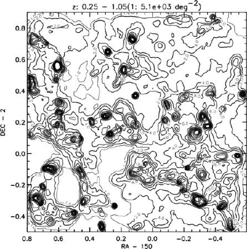
Figure 25: Application of the adaptive smoothing algorithm to the galaxies generated in the Millennium Simulation COSMOS light cone were processed identically to the observed galaxy distribution, including the imposition of redshift uncertainties like those in the observations and using the same smoothing parameters. The figure shows the projected distribution of overdensities integrated from z = 0.2 to 1.05 and with contours identical to those employed for the observations in Figure 5.

In our tests on the Millennium Simulation, the objective was to determine if similar structures were seen in this most up to date simulation as in the COSMOS data. Thus the galaxies in the MIllennium COSMOS light cone were each given a redshift uncertainty similar to that in the COSMOS photometric redshifts and then processed identically to the observed galaxies. In Figure 25 the overdensities from the simulation are integrated along the line of sight from z = 0.25 to 1.05 as was done for Figure 5, including keeping the same contours for both plots. Extremely good correspondence is seen from the comparison indicating that the adaptive smoothing is recovering very similar structures in both and by implication, both theory and observations have similar intrinsic structure. In Section 4, we make a more quantitative comparison by measuring the area filling factor as a function of overdensity and redshift.

Table 1: LSS Galaxy Samples

Sample	z	I cutoff (mag)	# of galaxies	# (early type)	# (late type)
all-z	z $\leq 3.$	26	487973	59285	428688
…	…	25	228487	34303	194184
…	…	24	106487	25278	81209
low-z	$z<$ 1.1	25	150162	25583	124579

Note. — All samples have M${}_{V}<-18$ and galaxies must be detected in at least 4 bands.

Table 2: Galaxy Selection ’Completeness’

Redshift interval	Rel. # per unit vol.	Rel. Mass per unit vol.
0.1 – 0.3	0.52	0.69
0.3 – 0.5	0.69	0.94
0.5 – 0.7	1.0	0.92
0.7 – 0.9	0.56	0.96
0.9 – 1.1	0.47	1.0

Note. — The total number of galaxies and total mass of galaxies per unit comoving volume were evaluated by integrating the distribution functions shown in right panel of Figure 2 at masses above 10⁹ $M_{\odot}$. These totals were normalized to the values in the redshift interval with the largest values in order to assess the count and mass incompleteness relative to this maximum bin.

Table 3:      Structures in the COSMOS field

				FWHM
Structure #	RA-150	Dec-2	z	$\Delta$RA	$\Delta$DEC	$\Delta$z	size	% LSS	# galaxies	M∗	Central $\Sigma_{1Mpc}$
(X-ray id)	(∘)	(∘)		(∘)	(∘)		Mpc			$10^{12}$$M_{\odot}$
1 (73,97,100,103,106)	-0.09	0.51	0.73	0.22	0.17	0.27	12.69	35	1767	23.63	188
2 (62,68,84)	0.15	0.20	0.88	0.26	0.21	0.25	17.41	30	815	15.72	99
3 (126,128)	-0.33	0.27	0.93	0.18	0.17	0.20	13.31	36	875	17.85	48
4	0.57	0.49	0.71	0.15	0.14	0.28	8.94	24	569	4.55	46
5	-0.49	-0.13	0.62	0.24	0.22	0.11	12.97	31	939	6.25	63
6 (40,45,53)	0.42	-0.14	0.92	0.16	0.17	0.19	12.70	33	580	11.51	47
7	0.30	0.40	0.73	0.14	0.13	0.21	8.70	25	384	3.97	84
8	0.40	0.77	0.75	0.25	0.10	0.18	12.30	27	526	4.93	96
9 (32)	0.51	0.23	0.89	0.12	0.12	0.18	9.25	40	512	10.32	57
10 (66,72)	0.16	0.60	0.87	0.25	0.15	0.26	15.48	32	394	6.76	59
11	0.27	-0.42	0.46	0.12	0.09	0.25	4.70	44	403	1.93	92
12	0.15	0.70	0.54	0.12	0.10	0.37	5.49	28	255	2.05	49
13 (25,64)	0.46	0.56	0.29	0.13	0.16	0.17	4.20	53	197	1.31	41
14	0.06	0.30	0.74	0.08	0.08	0.22	5.13	26	141	1.70	105
15 (111)	-0.23	0.32	0.34	0.14	0.15	0.11	4.81	44	168	1.47	54
16	-0.24	0.92	0.38	0.10	0.08	0.12	3.28	56	226	2.18	103
17 (78,85)	0.05	0.22	0.24	0.07	0.16	0.14	3.10	62	127	1.10	16
18	-0.50	0.01	0.98	0.10	0.09	0.11	7.57	31	102	2.07	16
19	0.53	0.73	0.22	0.18	0.11	0.10	3.39	60	77	0.59	12
20 (34,39,41,44)	0.49	0.07	0.45	0.05	0.05	0.18	2.07	53	133	1.19	104
21	0.20	-0.37	0.32	0.06	0.05	0.39	1.71	52	95	0.38	64
22 (89,105)	-0.08	0.60	0.26	0.06	0.14	0.11	2.81	62	67	0.71	42
23 (15)	0.45	0.05	0.33	0.05	0.08	0.10	2.19	57	82	0.56	58
24 (80)	0.11	0.56	0.61	0.03	0.04	0.26	1.97	43	85	0.82	131
25	-0.56	0.43	0.46	0.06	0.05	0.09	2.42	58	87	1.34	90
26 (145)	-0.60	0.57	0.39	0.05	0.03	0.12	1.49	67	92	0.78	131
27 (54,57,59)	0.33	-0.40	0.37	0.03	0.04	0.22	1.29	55	37	0.17	44
28 (70)	0.18	-0.24	0.30	0.03	0.06	0.24	1.40	59	43	0.37	39
29	-0.34	-0.44	0.45	0.07	0.03	0.21	2.27	35	31	0.05	22
30 (67)	0.34	-0.39	0.19	0.03	0.03	0.08	0.63	76	17	0.24	21
31 (132)	-0.41	0.82	0.32	0.03	0.02	0.06	0.77	72	22	0.49	31
32 (56)	0.10	-0.00	0.30	0.03	0.03	0.03	0.93	49	12	0.08	22
33	-0.31	0.35	0.20	0.03	0.03	0.03	0.57	91	9	0.01	–
34	0.39	0.87	0.16	0.02	0.01	0.05	0.24	86	3	0.09	–
35 (29,42)	0.53	0.49	0.16	0.01	0.01	0.05	0.23	85	2	0.03	–
36 (140)	-0.59	0.57	0.17	0.01	0.01	0.05	0.23	85	2	0.00	–
37	0.51	-0.45	0.20	0.01	0.01	0.00	0.29	86	3	0.02	–
38	-0.16	0.68	0.20	0.01	0.02	0.00	0.29	70	…	0.01	–
39	0.33	-0.36	0.60	0.01	0.01	0.00	0.63	36	…	0.01	10
40	0.74	0.67	0.90	0.01	0.01	0.03	0.77	29	…	0.02	–
41	0.65	0.31	0.30	0.01	0.01	0.00	0.28	38	…	0.02	–
42	-0.30	0.51	0.50	0.01	0.01	0.00	0.38	30	…	0.01	–

Table 4: Relative Variances for 2.5 deg² field

Redshift	Comoving Volume	M(vol)	$\sigma$(M(vol))	Halo mass	Number	$<b>$	$\sigma_{shot}$	$\sigma_{cosmic}$	$\sigma(M,z)$
range	$10^{6}$ present-day Mpc3	1017 $M_{\odot}$		range ($M_{\odot}$)	expected
0.2 – 0.4	0.80	0.327	0.149	$10^{13}$–$10^{14}$	142	1.62	0.084	0.240	0.254
0.2 – 0.4	0.80	0.327	0.149	$10^{14}$–$10^{15}$	6	3.03	0.397	0.451	0.601
0.4 – 0.6	1.78	0.727	0.099	$10^{13}$–$10^{14}$	279	1.84	0.060	0.182	0.192
0.4 – 0.6	1.78	0.727	0.099	$10^{14}$–$10^{15}$	10	3.52	0.324	0.349	0.476
0.6 – 0.8	2.79	1.14	0.075	$10^{13}$–$10^{14}$	372	2.09	0.052	0.157	0.165
0.6 – 0.8	2.79	1.14	0.075	$10^{14}$–$10^{15}$	9	4.08	0.327	0.307	0.448
0.8 – 1	3.67	1.50	0.061	$10^{13}$–$10^{14}$	405	2.37	0.050	0.145	0.153
0.8 – 1	3.67	1.50	0.061	$10^{14}$–$10^{15}$	7	4.71	0.371	0.288	0.470
1 – 1.2	4.40	1.79	0.052	$10^{13}$–$10^{14}$	387	2.69	0.051	0.140	0.149
1 – 1.2	4.40	1.79	0.052	$10^{14}$–$10^{15}$	5	5.41	0.458	0.282	0.538

Note. — The field size of 2.5 deg² was taken to match the area of the sample taken from the COSMOS photometric redshift catalog used here. The table includes the expected number of halos in two mass ranges, together with the relative variances due to shot noise, cosmic variance and the combined total variance. Values calculated for cosmological parameters : H₀ = 70 km s^-1 Mpc^-1, $\Omega_{M}$ = 0.3, $\Omega_{\Lambda}$ = 0.7 and $\sigma_{8}=0.74$.

Table 5: Parameters for Structures in Simulation

Structure #	RA	Dec	FWHM(′)	Peak (#/□∘)	# galaxies
1	-0.48	-0.64	1.0	6148	2
2	-0.16	-0.64	1.9	6148	8
3	0.16	-0.64	5.8	6148	65
4	0.48	-0.64	11.5	6148	252
5	-0.48	-0.24	1.0	18446	6
6	-0.16	-0.24	1.9	18446	22
7	0.16	-0.24	5.8	18446	194
8	0.48	-0.24	11.5	18446	773
9	-0.48	0.16	1.0	61489	18
10	-0.16	0.16	1.9	30744	36
11	0.16	0.16	5.8	30744	322
12	0.48	0.16	11.5	30744	1288
13	-0.42	0.58	1.0	43042	13
14	-0.48	0.64	1.9	24595	29
15	-0.48	0.58	5.8	24595	258
16	-0.09	0.58	1.9	24595	29
17	-0.16	0.67	1.9	24595	29
18	-0.16	0.58	7.7	12297	229
19	0.23	0.58	1.9	30744	36
20	0.16	0.64	5.8	18446	194
21	0.16	0.58	11.5	12297	514
22	0.48	0.64	1.9	24595	29
23	0.58	0.58	3.8	24595	115
24	0.48	0.58	8.7	12297	290

Note. — Total number of galaxies in all the stuctures is 4740.

Figure 1: a) Left : The number distribution of galaxies from the COSMOS photometric redshift catalog (Mobasher et al., 2006) is shown as a function of redshift in bins of width $\Delta z=0.2$ for different I-band magnitude cutoffs. b) Right : The widths of the derived photometric redshift probability distributions are shown as a function of z. The quantity plotted is the mean of 1.3$\times\sigma_{z}/(1+z)$ for the photo-z likelihood distributions for all galaxies in each redshift bin of $\Delta z=0.2$. For a Gaussian uncertainty distribution, 50% of the probability is within a full width of 1.3$\times\sigma_{z}$ of the peak. Galaxies used in this plot were selected to have M${}_{V}\leq-18$  mag and be detected in at least 4 bands.

Fig. 3. — cont’d

Fig. 3. — cont’d

Fig. 4. — cont’d

Fig. 4. — cont’d

Fig. 4. — cont’d

Fig. 4. — cont’d

Figure 6: The relative locations of each of the LSS are shown with their centroid redshifts.

Figure 7: The radial distribution of galaxies is shown for each structure using radius determined from the peak position of the number count distribution. The structures are ordered (as before) in decreasing numbers of pseudo 3-d space pixels. LSS above # 26 are not plotted since they have too few galaxies for a meaningful radial distribution. In all cases, the background galaxy distribution is removed. Many of the structures exhibit centrally peaked, well-behaved radial profiles, indicating candidate galaxy clusters with typical radii 1 – 2 Mpc. In cases where the LSS has multiple peaks of comparable amplitude, the radial distribution appears non-monotonic.

Fig. 7. — cont’d

Figure 8: a) Left : The distribution of total stellar masses for the structures are shown for masses $5\times 10^{11}$ to 10¹⁴ $M_{\odot}$. b) Right : The distribution of Richness measures for the the structures is shown, calculated as the surface density of galaxies brighter than 2 mag below the 3rd brightest galaxy (see text). Specifically, Richness is defined as the number of galaxies within the central R $\leq$ 1 Mpc brighter than 2 magnitudes fainter than the 3rd brightest galaxy within the cluster (i.e. M${}_{V}<$ M_V(3rd) + 2 ). Radius is measured from the location of peak surface density as in Figure 7.

Figure 9: The redshift distributions of summed structure masses are shown for redshift bins $\Delta z=0.25$. Uncertainties due to Poisson and cosmic variance are comparable and the expected total relative variance in these number distributions is 40-60% (i.e. $\sigma_{N}/N\sim 0.5$; see Section 3.5 and Table 4). The dotted line plots the relative comoving volumes for the selected redshift bins, with vertical scale arbitrarily normalized – simply to indicate that the overall distribution of structure mass with redshift is consistent with the expected mass conservation. The apparent discrepancy in the lowest redshift bin is probably not significant given the very large variances noted above.

Figure 10: The cumulative mass function ($n(>M)=\int_{M}^{\infty}n(m)\,dm$) is shown for the 42 COSMOS LSS with linear mass bins of width $\Delta M_{*}=2\times 10^{12}$ $M_{\odot}$. Also shown are the cumulative mass functions derived from optical and X-ray studies as summarized by (Reiprich & Böhringer, 2002). The mass function for masses within the Abell radius of each cluster is shown by the triangle symbols (M_A); masses within the regions with density exceeding 200$\rho_{c}$ and 500$\rho_{c}$ (where $\rho_{c}$ is the critical density for the universe) are shown by the squares and crosses (see Reiprich & Böhringer, 2002). The expected cosmic variance and Poisson noise are included in the error bars (see Section 3.5 and Table 4).

References

- Abell (1958) Abell, G. O. 1958, ApJS, 3, 211
- Bahcall & Cen (1993) Bahcall, N. A. & Cen, R. 1993, ApJ, 407, L49
- Bell et al. (2005) Bell, E. F., Papovich, C., Wolf, C., Le Floc’h, E., Caldwell, J. A. R., Barden, M., Egami, E., McIntosh, D. H., Meisenheimer, K., Pérez-González, P. G., Rieke, G. H., Rieke, M. J., Rigby, J. R., & Rix, H.-W. 2005, ApJ, 625, 23
- Benítez (2000) Benítez, N. 2000, ApJ, 536, 571
- Benson et al. (2000) Benson, A. J., Cole, S., Frenk, C. S., Baugh, C. M., & Lacey, C. G. 2000, MNRAS, 311, 793
- Benson et al. (2001) Benson, A. J., Frenk, C. S., Baugh, C. M., Cole, S., & Lacey, C. G. 2001, MNRAS, 327, 1041
- Borch et al. (2006) Borch, A., Meisenheimer, K., Bell, E. F., Rix, H.-W., Wolf, C., Dye, S., Kleinheinrich, M., Kovacs, Z., & Wisotzki, L. 2006, A&A, 453, 869
- Bower et al. (2006) Bower, R. G., Benson, A. J., Malbon, R., Helly, J. C., Frenk, C. S., Baugh, C. M., Cole, S., & Lacey, C. G. 2006, MNRAS, 370, 645
- Bundy et al. (2005) Bundy, K., Ellis, R. S., Conselice, C. J., Taylor, J. E., Cooper, M. C., Willmer, C. N. A., Weiner, B. J., Coil, A. L., Noeske, K. G., & Eisenhardt, P. R. M. 2005, ArXiv Astrophysics e-prints
- Butcher & Oemler (1984) Butcher, H. & Oemler, Jr., A. 1984, ApJ, 285, 426
- Capak (2006) Capak, P. 2006, ApJ, xxx-xxx
- Capak et al. (2006) Capak, P., Aussel, H., Ajiki, M., McCracken, H. J., Mobasher, B., Scoville, N., Shopbell, P., Taniguchi, Y., Thompson, D., Tribiano, S., Sasaki, T., Blain, A. W., Brusa, M., Carilli, C. L., Carollo, C. M., Ellis, R. S., Elvis, M., Giavalisco, M., Green, W., Guzzo, L., Hasinger, G., Impey, C. D., Ilbert, O., & Jahnke, K. e. 2006, ApJ, xxx-xxx
- Cassata (2006) Cassata, P. 2006, ApJ, xxx-xxx
- Cen & Ostriker (1993) Cen, R. & Ostriker, J. P. 1993, ApJ, 417, 415
- Coil et al. (2006) Coil, A. L., Gerke, B. F., Newman, J. A., Ma, C.-P., Yan, R., Cooper, M. C., Davis, M., Faber, S. M., Guhathakurta, P., & Koo, D. C. 2006, ApJ, 638, 668
- Cooper et al. (2006) Cooper, M. C., Newman, J. A., Croton, D. J., Weiner, B. J., Willmer, C. N. A., Gerke, B. F., Madgwick, D. S., Faber, S. M., Davis, M., Coil, A. L., Finkbeiner, D. P., Guhathakurta, P., & Koo, D. C. 2006, MNRAS, 370, 198
- Cowie et al. (1996) Cowie, L. L., Songaila, A., Hu, E. M., & Cohen, J. G. 1996, AJ, 112, 839
- Croton et al. (2006) Croton, D. J., Springel, V., White, S. D. M., De Lucia, G., Frenk, C. S., Gao, L., Jenkins, A., Kauffmann, G., Navarro, J. F., & Yoshida, N. 2006, MNRAS, 365, 11
- Dahlen et al. (2005) Dahlen, T., Mobasher, B., Somerville, R. S., Moustakas, L. A., Dickinson, M., Ferguson, H. C., & Giavalisco, M. 2005, ApJ, 631, 126
- Davis & Geller (1976) Davis, M. & Geller, M. J. 1976, ApJ, 208, 13
- Davis et al. (2006) Davis, M., Guhathakurta, P., Konidaris, N., Newman, J. A., Ashby, M. L. N., Biggs, A. D., Barmby, P., Bundy, K., Chapman, S., Coil, A. L., Conselice, C., Cooper, M., Croton, D., Eisenhardt, P., Ellis, R., Faber, S., Fang, T., Fazio, G. G., Georgakakis, A., Gerke, B., Goss, W. M., Gwyn, S., Harker, J., Hopkins, A., Huang, J. ., Ivison, R. J., Kassin, S. A., Kirby, E., Koekemoer, A., Koo, D. C., Laird, E., Le Floc’h, E., Lin, L., Lotz, J., Marshall, P. J., Martin, D. C., Metevier, A., Moustakas, L. A., Nandra, K., Noeske, K., Papovich, C., Phillips, A. C., Rich, R. M., Rieke, G. H., Rigopoulou, D., Salim, S., Schiminovich, D., Simard, L., Smail, I., Small, T. A., Weiner, B., Willmer, C. N. A., Willner, S. P., Wilson, G., Wright, E., & Yan, R. 2006, ArXiv Astrophysics e-prints
- De Lucia et al. (2004) De Lucia, G., Poggianti, B. M., Aragón-Salamanca, A., Clowe, D., Halliday, C., Jablonka, P., Milvang-Jensen, B., Pelló, R., Poirier, S., Rudnick, G., Saglia, R., Simard, L., & White, S. D. M. 2004, ApJ, 610, L77
- Dressler et al. (1997) Dressler, A., Oemler, A. J., Couch, W. J., Smail, I., Ellis, R. S., Barger, A., Butcher, H., Poggianti, B. M., & Sharples, R. M. 1997, ApJ, 490, 577
- Drory et al. (2005) Drory, N., Salvato, M., Gabasch, A., Bender, R., Hopp, U., Feulner, G., & Pannella, M. 2005, ApJ, 619, L131
- Ebeling & Wiedenmann (1993) Ebeling, H. & Wiedenmann, G. 1993, Phys. Rev. E, 47, 704
- Escalera & MacGillivray (1995) Escalera, E. & MacGillivray, H. T. 1995, A&A, 298, 1
- Finoguenov et al. (2006) Finoguenov, A., Guzzo, L., Hasinger, G., Scoville, N. Z., Aussel, H., Böhringer, H., Brusa, M., Capak, P., Cappelluti, N., Comastri, A., Griffiths, R., Impey, C., Koekemoer, A., Kneib, J.-P., Leauthaud, A., Le Fèvre, O., Lilly, S., Massey, R., Mobasher, B., Mainieri, V.and Peacock, J., Sakelliou, I., Schinnerer, E., Silverman, J., Smolčić, V., Tasca, L., Taylor, J., Trump, J., & Zamorani, G. 2006, ApJ, xxx-xxx
- Gerke et al. (2005) Gerke, B. F., Newman, J. A., Davis, M., Marinoni, C., Yan, R., Coil, A. L., Conroy, C., Cooper, M. C., Faber, S. M., Finkbeiner, D. P., Guhathakurta, P., Kaiser, N., Koo, D. C., Phillips, A. C., Weiner, B. J., & Willmer, C. N. A. 2005, ApJ, 625, 6
- Gladders & Yee (2005) Gladders, M. D. & Yee, H. K. C. 2005, ApJS, 157, 1
- Guzik & Seljak (2002) Guzik, J. & Seljak, U. 2002, MNRAS, 335, 311
- Guzzo & Cassata (2006) Guzzo, L. & Cassata, P. e. 2006, ApJ, xxx-xxx
- Helly et al. (2003) Helly, J. C., Cole, S., Frenk, C. S., Baugh, C. M., Benson, A., & Lacey, C. 2003, MNRAS, 338, 903
- Hoekstra et al. (2006) Hoekstra, H., Mellier, Y., van Waerbeke, L., Semboloni, E., Fu, L., Hudson, M. J., Parker, L. C., Tereno, I., & Benabed, K. 2006, ApJ, 647, 116
- Hopkins (2004) Hopkins, A. M. 2004, ApJ, 615, 209
- Impey (2006) Impey, C. D. e. 2006, ApJ, xxx-xxx
- Juneau et al. (2005) Juneau, S., Glazebrook, K., Crampton, D., McCarthy, P. J., Savaglio, S., Abraham, R., Carlberg, R. G., Chen, H.-W., Le Borgne, D., Marzke, R. O., Roth, K., Jørgensen, I., Hook, I., & Murowinski, R. 2005, ApJ, 619, L135
- Kaiser (1984) Kaiser, N. 1984, ApJ, 282, 374
- Kauffmann et al. (1999) Kauffmann, G., Colberg, J. M., Diaferio, A., & White, S. D. M. 1999, MNRAS, 303, 188
- Kauffmann et al. (2004) Kauffmann, G., White, S. D. M., Heckman, T. M., Ménard, B., Brinchmann, J., Charlot, S., Tremonti, C., & Brinkmann, J. 2004, MNRAS, 353, 713
- Kinney et al. (1996) Kinney, A. L., Calzetti, D., Bohlin, R. C., McQuade, K., Storchi-Bergmann, T., & Schmitt, H. R. 1996, ApJ, 467, 38
- Kodama et al. (2004) Kodama, T., Yamada, T., Akiyama, M., Aoki, K., Doi, M., Furusawa, H., Fuse, T., Imanishi, M., Ishida, C., Iye, M., Kajisawa, M., Karoji, H., Kobayashi, N., Komiyama, Y., Kosugi, G., Maeda, Y., Miyazaki, S., Mizumoto, Y., Morokuma, T., Nakata, F., Noumaru, J., Ogasawara, R., Ouchi, M., Sasaki, T., Sekiguchi, K., Shimasaku, K., Simpson, C., Takata, T., Tanaka, I., Ueda, Y., Yasuda, N., & Yoshida, M. 2004, MNRAS, 350, 1005
- Kolb & Turner (1990) Kolb, E. W. & Turner, M. S. 1990, The early universe (Frontiers in Physics, Reading, MA: Addison-Wesley, 1988, 1990)
- Le Fèvre et al. (2005) Le Fèvre, O., Guzzo, L., Meneux, B., Pollo, A., Cappi, A., Colombi, S., Iovino, A., Marinoni, C., McCracken, H. J., Scaramella, R., Bottini, D., Garilli, B., Le Brun, V., Maccagni, D., Picat, J. P., Scodeggio, M., Tresse, L., Vettolani, G., Zanichelli, A., Adami, C., Arnaboldi, M., Arnouts, S., Bardelli, S., Blaizot, J., Bolzonella, M., Charlot, S., Ciliegi, P., Contini, T., Foucaud, S., Franzetti, P., Gavignaud, I., Ilbert, O., Marano, B., Mathez, G., Mazure, A., Merighi, R., Paltani, S., Pellò, R., Pozzetti, L., Radovich, M., Zamorani, G., Zucca, E., Bondi, M., Bongiorno, A., Busarello, G., Lamareille, F., Mellier, Y., Merluzzi, P., Ripepi, V., & Rizzo, D. 2005, A&A, 439, 877
- Lilly (2006) Lilly, S. J. e. 2006, ApJ, xxx-xxx
- Madau et al. (1996) Madau, P., Ferguson, H. C., Dickinson, M. E., Giavalisco, M., Steidel, C. C., & Fruchter, A. 1996, MNRAS, 283, 1388
- Marinoni et al. (2002) Marinoni, C., Davis, M., Newman, J. A., & Coil, A. L. 2002, ApJ, 580, 122
- Massey (2006) Massey, R. 2006, ApJ, xxx-xxx
- McCracken (2006) McCracken, H. J. 2006, ApJ, xxx-xxx
- Meneux et al. (2006) Meneux, B., Le Fèvre, O., Guzzo, L., Pollo, A., Cappi, A., Ilbert, O., Iovino, A., Marinoni, C., McCracken, H. J., Bottini, D., Garilli, B., Le Brun, V., Maccagni, D., Picat, J. P., Scaramella, R., Scodeggio, M., Tresse, L., Vettolani, G., Zanichelli, A., Adami, C., Arnouts, S., Arnaboldi, M., Bardelli, S., Bolzonella, M., Charlot, S., Ciliegi, P., Contini, T., Foucaud, S., Franzetti, P., Gavignaud, I., Marano, B., Mazure, A., Merighi, R., Paltani, S., Pellò, R., Pozzetti, L., Radovich, M., Zamorani, G., Zucca, E., Bondi, M., Bongiorno, A., Busarello, G., Cucciati, O., Gregorini, L., Lamareille, F., Mathez, G., Mellier, Y., Merluzzi, P., Ripepi, V., & Rizzo, D. 2006, A&A, 452, 387
- Mo & White (1996) Mo, H. J. & White, S. D. M. 1996, MNRAS, 282, 347
- Mobasher et al. (2006) Mobasher, B., Capak, P., Scoville, N., Dahlen, T., Salvato, M., Aussel, H., Thompson, D., & Feldman, R. 2006, ApJ, xxx-xxx
- Mobasher (2006) Mobasher, B. e. 2006, ApJ, xxx-xxx
- O’Hely et al. (1998) O’Hely, E., Couch, W. J., Smail, I., Edge, A. C., & Zabludoff, A. 1998, Publications of the Astronomical Society of Australia, 15, 273
- Pimbblet et al. (2006) Pimbblet, K. A., Smail, I., Edge, A. C., O’Hely, E., Couch, W. J., & Zabludoff, A. I. 2006, MNRAS, 366, 645
- Postman et al. (2005) Postman, M., Franx, M., Cross, N. J. G., Holden, B., Ford, H. C., Illingworth, G. D., Goto, T., Demarco, R., Rosati, P., Blakeslee, J. P., Tran, K.-V., Benítez, N., Clampin, M., Hartig, G. F., Homeier, N., Ardila, D. R., Bartko, F., Bouwens, R. J., Bradley, L. D., Broadhurst, T. J., Brown, R. A., Burrows, C. J., Cheng, E. S., Feldman, P. D., Golimowski, D. A., Gronwall, C., Infante, L., Kimble, R. A., Krist, J. E., Lesser, M. P., Martel, A. R., Mei, S., Menanteau, F., Meurer, G. R., Miley, G. K., Motta, V., Sirianni, M., Sparks, W. B., Tran, H. D., Tsvetanov, Z. I., White, R. L., & Zheng, W. 2005, ApJ, 623, 721
- Postman & Geller (1984) Postman, M. & Geller, M. J. 1984, ApJ, 281, 95
- Postman et al. (1996) Postman, M., Lubin, L. M., Gunn, J. E., Oke, J. B., Hoessel, J. G., Schneider, D. P., & Christensen, J. A. 1996, AJ, 111, 615
- Reiprich & Böhringer (2002) Reiprich, T. H. & Böhringer, H. 2002, ApJ, 567, 716
- Rix et al. (2004) Rix, H.-W., Barden, M., Beckwith, S. V. W., Bell, E. F., Borch, A., Caldwell, J. A. R., Häussler, B., Jahnke, K., Jogee, S., McIntosh, D. H., Meisenheimer, K., Peng, C. Y., Sanchez, S. F., Somerville, R. S., Wisotzki, L., & Wolf, C. 2004, ApJS, 152, 163
- Sanders (2006) Sanders, D. B. e. 2006, ApJ, xxx-xxx
- Schiminovich et al. (2005) Schiminovich, D., Ilbert, O., Arnouts, S., Milliard, B., Tresse, L., Le Fèvre, O., Treyer, M., Wyder, T. K., Budavári, T., Zucca, E., Zamorani, G., Martin, D. C., Adami, C., Arnaboldi, M., Bardelli, S., Barlow, T., Bianchi, L., Bolzonella, M., Bottini, D., Byun, Y.-I., Cappi, A., Contini, T., Charlot, S., Donas, J., Forster, K., Foucaud, S., Franzetti, P., Friedman, P. G., Garilli, B., Gavignaud, I., Guzzo, L., Heckman, T. M., Hoopes, C., Iovino, A., Jelinsky, P., Le Brun, V., Lee, Y.-W., Maccagni, D., Madore, B. F., Malina, R., Marano, B., Marinoni, C., McCracken, H. J., Mazure, A., Meneux, B., Morrissey, P., Neff, S., Paltani, S., Pellò, R., Picat, J. P., Pollo, A., Pozzetti, L., Radovich, M., Rich, R. M., Scaramella, R., Scodeggio, M., Seibert, M., Siegmund, O., Small, T., Szalay, A. S., Vettolani, G., Welsh, B., Xu, C. K., & Zanichelli, A. 2005, ApJ, 619, L47
- Schuecker & Boehringer (1998) Schuecker, P. & Boehringer, H. 1998, A&A, 339, 315
- Scoville (2006a) Scoville, N. Z. 2006a, ApJ, xxx-xxx
- Scoville (2006b) —. 2006b, ApJ, xxx-xxx
- Sheth & Tormen (1999) Sheth, R. K. & Tormen, G. 1999, MNRAS, 308, 119
- Smith et al. (2005) Smith, G. P., Treu, T., Ellis, R. S., Moran, S. M., & Dressler, A. 2005, ApJ, 620, 78
- Smolčić (2006) Smolčić, V. e. 2006, ApJ, xxx
- Somerville et al. (2004) Somerville, R. S., Lee, K., Ferguson, H. C., Gardner, J. P., Moustakas, L. A., & Giavalisco, M. 2004, ApJ, 600, L171
- Spergel et al. (2006) Spergel, D. N., Bean, R., Dore’, O., Nolta, M. R., Bennett, C. L., Hinshaw, G., Jarosik, N., Komatsu, E., Page, L., Peiris, H. V., Verde, L., Barnes, C., Halpern, M., Hill, R. S., Kogut, A., Limon, M., Meyer, S. S., Odegard, N., Tucker, G. S., Weiland, J. L., Wollack, E., & Wright, E. L. 2006, ArXiv Astrophysics e-prints
- Springel et al. (2005) Springel, V., White, S. D. M., Jenkins, A., Frenk, C. S., Yoshida, N., Gao, L., Navarro, J., Thacker, R., Croton, D., Helly, J., Peacock, J. A., Cole, S., Thomas, P., Couchman, H., Evrard, A., Colberg, J., & Pearce, F. 2005, Nature, 435, 629
- Taniguchi et al. (2006) Taniguchi, Y., Scoville, N. Z., Ajiki, M., Sanders, D. B., Mobasher, B., Aussel, H., & Capak, P. 2006, ApJ, xxx-xxx
- van de Weygaert (1994) van de Weygaert, R. 1994, A&A, 283, 361
- van den Bosch et al. (2003) van den Bosch, F. C., Yang, X., & Mo, H. J. 2003, MNRAS, 340, 771
- Williams et al. (1994) Williams, J. P., de Geus, E. J., & Blitz, L. 1994, ApJ, 428, 693